the Creative Commons Attribution 4.0 License.
the Creative Commons Attribution 4.0 License.
 | 07 May 2019
Mesospheric semidiurnal tides and near-12 h waves through jointly analyzing observations of five specular meteor radars from three longitudinal sectors at boreal midlatitudes
Jorge Luis Chau
In the last decades, mesospheric tides have been intensively investigated with observations from both ground-based radars and satellites. Single-site radar observations provide continuous measurements at fixed locations without horizontal information, whereas single-spacecraft missions typically provide global coverage with limited temporal coverage at a given location. In this work, by combining 8 years (2009–2016) of mesospheric winds collected by five specular meteor radars from three different longitudinal sectors at boreal midlatitudes (49±8.5∘ N), we develop an approach to investigate the most intense global-scale oscillation, namely at the period h. Six waves are resolved: the semidiurnal westward-traveling tidal modes with zonal wave numbers 1, 2, and 3 (SW1, SW2, SW3), the lunar semidiurnal tide M2, and the upper and lower sidebands (USB and LSB) of the 16 d wave nonlinear modulation on SW2. The temporal variations of the waves are studied statistically with a special focus on their responses to sudden stratospheric warming events (SSWs) and on their climatological seasonal variations. In response to SSWs, USB, LSB, and M2 enhance, while SW2 decreases. However, SW1 and SW3 do not respond noticeably to SSWs, contrary to the broadly reported enhancements in the literature. The USB, LSB, and SW2 responses could be explained in terms of energy exchange through the nonlinear modulation, while LSB and USB might previously have been misinterpreted as SW1 and SW3, respectively. Besides, we find that LSB and M2 enhancements depend on the SSW classification with respect to the associated split or displacement of the polar vortex. In the case of seasonal variations, our results are qualitatively consistent with previous studies and show a moderate correlation with an empirical tidal model derived from satellite observations.
- Article
(5205 KB) - Full-text XML
- BibTeX
- EndNote


The availability of observations limits the advancement of studies on the mesosphere–lower-thermosphere (MLT). In situ MLT observations are available, e.g., through rockets, only on campaign bases, whereas remote detection allows MLT to be monitored perennially and continuously. Two most common approaches of the remote detection are ground-based radars with all-weather applicability and satellite-based optical instruments with good mobility.
Both continuous ground- and space-based observations have been used to investigate the global-scale MLT waves. Most of these studies were based on single-point analysis techniques and therefore were subject to inherent spatiotemporal ambiguities (following Paschmann and Daly, 1998, here “point” refers to a geometric element, either stationary or moving, has no extension in the space). Ground-based observations from single radars could yield high-frequency-resolved spectra of MLT parameters but cannot resolve the global-scale structure (e.g., Azeem et al., 2000). On the other hand, space-based sensors, typically on-board slowly precessing polar satellites (e.g., Oberheide et al., 2002), collect data with global coverage but with limited temporal coverage for given locations. They are capable of determining the horizontal scales, which, however, cannot distinguish instantaneous temporal variations from spatial variations. The obtained frequency spectra are usually Doppler shifted at limited resolution (e.g., Salby, 1982a, b) under the assumption that the tides are static.
To overcome the spatiotemporal ambiguity, specular meteor radars (SMRs) or medium-frequency radars from multi-longitudinal sectors had been combined to resolve the horizontal scale of MLT waves at polar latitudes tentatively. A typical procedure is a least square regression (LSR) fitting of longitudinal harmonic functions with preassigned wave number to observations from different longitude sectors (e.g., Murphy, 2003). The LSR procedure was used to decompose the most significant global-scale periodicity, namely the 12 h tidal oscillation, into the migrating mode, SW2 (SWm represents westward-traveling semidiurnal tidal modes with zonal wave number m), and nonmigrating modes, SW1 and SW3 (mostly at polar latitudes, e.g., Murphy, 2003; Murphy et al., 2006, 2009; Baumgaertner et al., 2006; Manson et al., 2009). However, as sketched in Fig. 1, such decomposition is complicated by the existence of other waves in the vicinity of 12 h with wave numbers identical to those of solar tides. These include the semidiurnal lunar tide (M2) and the lower and upper sidebands (LSB and USB) of the nonlinear modulation of the 16 d planetary wave on SW2. Sharing similar periods and same wave numbers with the tides, these waves are suspected to have contaminated the interpretation of previous studies. Specifically, LSB and USB might have been detected at low-frequency resolutions and misinterpreted as SW1 and SW3 (cf. He et al., 2018a, b), respectively. Additionally, the M2 estimations might have been contaminated by LSB in spectral studies using the single-site observational technique (as explained in He et al., 2017) or by the power leakage from SW2 in low-frequency-resolved spectral analyses (cf. Sect. 5.1 in He et al., 2018b).

The main purpose of the current study is to develop an approach to unambiguously separate all six waves sketched in Fig. 1 using observations of five SMRs at latitudes near 49∘ N between 2009 and 2016. Below, Sect. 2 introduces the six waves and the approach. The results are shown in Sect. 3 and used to investigate the six waves statistically, in particular their responses to sudden stratospheric warming events (SSWs) and their seasonal variations (Sects. 4 and 5). Note that, in the current study, we use the term “responses to SSWs” to refer to the behaviors associated with SSW, which does not imply causative relations between the behaviors and the phenomenon suggested literally by the term “SSWs”, namely the sudden increase in the temperature.
For the current study, we collect the mesospheric wind observations of SMRs at 49±8.5∘ N from three longitudinal sectors, namely east Asia, Europe, and America. As shown in Figure 2, these SMRs are located at Juliusruh (12∘ E, 55∘ N, available since 2007), Collm (13∘ E, 51∘ N, since 2004), Beijing (116∘ E, 40∘ N, since 2009), Mohe (123∘ E, 54∘ N, since 2012), and Tavistock (81∘ W, 43∘ N, since 2002). The radar system at Tavistock is officially known as the Canadian Meteor Orbit Radar (CMOR, e.g., Jones et al., 2005). For details of the radars, e.g., working frequency, power, and configuration of antennas, readers are referred to Liu et al. (2016, 2017), Yu et al. (2013), Singer et al. (2013), Jacobi (2012), and Jones et al. (2005).
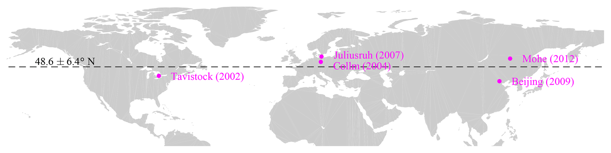
Figure 2Distribution of five SMRs used in the current study. The numbers following the location names present the earliest available years of the corresponding observations.
The current study uses hourly zonal wind derived at a vertical resolution of 2 km according to the algorithm introduced by Hocking et al. (2001) and Stober et al. (2012). For each SMR, we filter oscillations in the wind at periods 11.6±0.1, 12.0±0.1, and 12.4±0.1 h, through high-frequency-resolved wavelet spectral analysis. For each period, we decompose the potential waves with different wave numbers by jointly analyzing the spectral coherency between the SMRs.
2.1 Decomposition approach
A Morlet wavelet analysis is applied to the zonal wind at a given altitude for each SMR, resulting in spectra , where f, t, and represent the frequency, time, and an index of SMRs. corresponds to the phasor representation used (e.g., Murphy, 2002; Baumgaertner et al., 2006). We attribute the coherence among to waves traveling in the longitudinal direction with zonal wave number mk, () and complex amplitude . At given f and t, we fit from following Eq. (5) in He et al. (2018a).
Here, the kth entry of is defined as , and the entry of in the kth row and nth column is defined as , representing the phase of kth wave detected by the nth SMR at longitude λn. When , Eq. (1) allows to be estimated with preassigned mk, as demonstrated in Fig. 4 in He et al. (2018a). Since our five SMRs are mainly from three distinct longitudinal sectors, our implementation entails K≤3. Although two of the five radars provide redundant information as they are in the same longitude sector as other SMRs, we use all five for a broader temporal coverage and higher statistical significance. We assign m following Fig. 1 for reasons detailed in Sect. 2.2.
Note that in estimating , we assume that the meridional variation of all waves is negligible among the SMRs. To test this assumption, we ran the climatological tidal model of the thermosphere (CTMT, Oberheide et al., 2011) derived from TIDI and SABER. Semidiurnal components in the zonal wind at 50∘ N are highly correlated with those at 40∘ N: the correlation coefficients associated with SW2 and SW1 are 0.94 and 0.99 (not shown here). For the latitude dependence of the semidiurnal tide and its seasonal variation, readers are referred to Yu et al. (2015) and Oberheide et al. (2011), for example.
In principle, could be estimated through the LSR or a short-time Fourier transform (STFT) within a sliding window (e.g., Murphy, 2003; Baumgaertner et al., 2006). Using a Gaussian window with the proper width, the LSR or STFT might even yield results identical to ours. The width of the window, ΔT, proportionally determines the time resolution σt∝ΔT, which is coupled with the frequency resolution σf according to the Fabor's uncertainty principle . The resolution in our wavelet analysis is determined by the Morlet factor as specified in Sect. 2.2.
2.2 Targeting waves and assignment of zonal wave number
Tides are characterized by oscillations at periods which are integral fractions of a solar or lunar day. In the atmosphere, the solar tides are primarily forced by daily variation in the absorption of sunlight (Chapman and Lindzen, 1970). At a period of 12 h, the migrating component SW2 is known to be the dominant tide (e.g., Pancheva and Mukhtarov, 2012), while the nonmigrating components, SW1 and SW3, are also frequently reported (e.g., Angelats I Coll and Forbes, 2002; Manson et al., 2009). At the latitude for our study (49∘ N), SW1 and SW3 are expected to be more intensive than other semidiurnal nonmigrating tides on climatological averages (not shown here) according to the tidal model (cf. Oberheide et al., 2011). These solar tides, according to the classic tidal theory (Chapman and Lindzen, 1970), have amplitudes ∼20 times larger than those of lunar gravitationally forced tides. Despite these theoretical predictions, oscillations at 12.4 h have been clearly detected in the upper atmosphere and ionosphere and explained as the lunar tide M2, particularly around SSWs (e.g., Stening, 2011; Fejer et al., 2011; Chau et al., 2015). The occurrence of M2 was also confirmed by a wave number identification using a dual-SMR network (m=2 at 12.4 h during SSW 2013, cf. He et al., 2018b). The significant M2 tide was attributed to the lunar forcing resonance due to a shift of a local maximum (namely the Pekeris peak) in the atmospheric frequency response, which is supported by a comparison in a numerical experiment using GSWM driven by two specifications of a climatological-mean background atmosphere and that during SSWs (Forbes and Zhang, 2012).
In addition to the M2, also oscillating at the period 12.4 h is a westward-traveling structure with zonal wave number m=1, namely the lower sideband (LSB) of the modulation of the 16 d planetary wave (PW) on SW2 tide (as explicitly detected and explained in He et al., 2018a). LSB's m and f are determined by their parent waves according to the nonlinear interaction resonance conditions . Here, represents the phase of a wave • (e.g., He et al., 2017). The 16 d PW is a normal wave, and its intrinsic period of 12.5 d is determined by the resonant properties of the atmosphere (e.g., Ahlquist, 1982; Longuet-Higgins, 1968; Madden, 2007; Salby, 1984). Having been Doppler shifted by the prevailing eastward wind during winter, the PW is observed at a period up to 20 d, with an average of 16 d (for the climatology of the 16 d PW, cf. Luo et al., 2002; Day and Mitchell, 2010). The corresponding LSB occurs in the frequency range of , associated with LSB at h. Similarly to LSB, an upper sideband (USB), at h and m=3, might also be excited by the modulation, following the resonance conditions (as explicitly detected in He et al., 2018a). To include the periods of most potential LSB and USB, in our wavelet analysis (cf. Grossmann et al., 1990), we set the Morlet factor to 128 so that the passed frequency band corresponds to 12.4±0.1, 11.6±0.1 h, and 12.0±0.1 h. These period bands are narrow enough to prevent power leakage or aliasing between each other.
As sketched in Fig. 1, the abovementioned six waves occupy three near-12 h periods associated with three zonal wave numbers. When implementing Eq. (1) to quantify the waves, we assume that in comparison with the mentioned waves, other potential waves are negligible at each of the periods. Specifically, we assume that at h the most important waves are tides SW1, SW2, and SW3 (m1=1, m2=2 and m3=3); at h M2 and LSB are dominant (m1=1 and m2=2); and at h only the USB (m1=3) exists. With these assignments of m and according to Eq. (1), we repeat the estimation of on the grids of date t and altitude h at each of the three periods, resulting in the amplitudes for all six waves, , where • represents LSB, M2, the USB, SW1, SW2, or SW3. The corresponding amplitude is displayed in Fig. 3.

Figure 3(a) The amplitude of the lower sideband (LSB) of the nonlinear modulation of the 16 d wave on the semidiurnal tide SW2 as a function of time and altitude. (b–f) The same plots as (a) but for the lunar tide M2, the upper sideband (USB), and the solar tides, SW1, SW2, and SW3. (g) The altitude averages of panels (a), (b), and (c) (LSB, M2, and USB), and (h) those of panels (a), (b), and (c) (SW1, SW2, and SW3). In each panel, the solid white vertical lines display the first day of each year, and the dashed magenta lines display PVWs. In (f), the cyan line on the bottom illustrates the interval from 2012 to 2016 in which all decomposition is based on five SMRs, whereas the yellow line represents that MSR observations are not available at Mohe. In (a)–(c), the magenta plus symbols illustrate the maximum amplitude in each 30 d window following each PVW.
In Fig. 3, the decomposition is based on observations from five SMRs between 2012 and 2016, whereas before 2012 only four SMRs are available (Mohe SMR started operation in 2012). The different SMR combinations are designated by the yellow and cyan lines at the bottom of Fig. 3f. Using the four SMRs, we also produced the results between 2012 and 2016, which are highly consistent with the results from the five SMRs: the corresponding correlation coefficients are 0.92, 0.96, 0.93, 0.95, 0.98, and 0.95 for the six components. In Fig. 3a–c, the horizontal yellow line around January 2013 shows that the amplitudes are quantitatively consistent with the recent estimation using only the two SMRs at Juliusruh and Mohe: the components m=1, 2, and 3 maximize at roughly 4, 8, and 8 m s−1 in both Fig. 3a–c here and Fig. 4 in He et al. (2018b). The correlation and consistency suggest that the decomposition is not sensitive to the absence of one SMR between 2009 and 2011.
The temporal variations in Fig. 3a–f share some similarities. First, in Fig. 3a–c LSB, USB, and M2 are often enhanced noticeably in the month following the vertical dashed magenta lines which indicate the polar vortex weakening (PVW, cf. Zhang and Forbes, 2014) as a reference of SSWs in the current study. Second, as shown in Fig. 3d–f, SW1, SW2, and SW3 are characterized by repeating annual patterns, as separated by the calendar year indicated by the solid white lines. For a statistical study on the SSW responses and the seasonal variations, we average the amplitudes of the six components with respect to the time since the PVW epoch and day of year (DoY), respectively, following the composite analysis approach (CA, e.g., Chau et al., 2015). CA is also known as a superposed epoch analysis, SEA, in geophysics and solar physics (e.g., Chree, 1914). The PVW and calendar results are shown in Fig. 4 and discussed in Sects. 4 and 5.
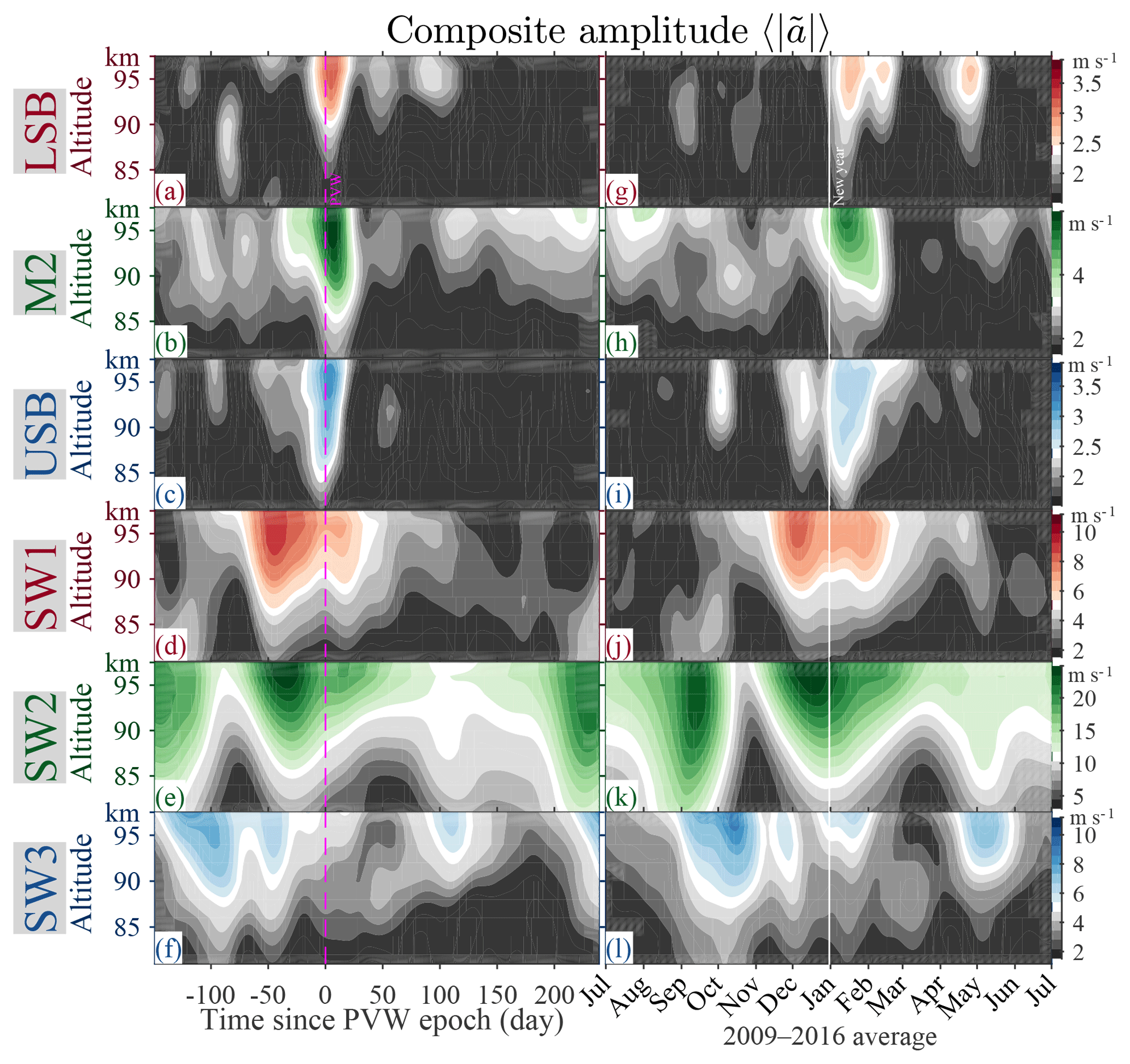
Figure 4(a) Composite analysis of LSB from Fig. 3a with respect to the occurrence of PVWs, namely the dashed magenta lines in Fig. 3a. (b–f) Same plots as (a) but for M2, USB, SW1, SW2, and SW3 from Fig. 3b–f. (g–l) Same plots as (a)–(f) but with respect to the start of the calendar years, namely the white lines in Fig. 3.
As the most radical manifestation of stratosphere–troposphere coupling, SSWs impact the upper atmosphere in broad altitude and latitude ranges (e.g., Goncharenko and Zhang, 2008; Goncharenko et al., 2013). One type of impact is the broadly reported enhancements of various waves at periods near 12 h, including M2, SW1, SW3, LSB and USB (e.g., Chau et al., 2015; Angelats I Coll and Forbes, 2002; Liu et al., 2010, and references therein). Recently, He et al. (2017) argued that there might not be SW1 and SW3 enhancements during SSWs and instead suggested that the reported enhancements are just misinterpreted signatures of LSB and USB at low-frequency resolution. These arguments about SW1 and SW3 were supported observationally by two case studies (He et al., 2018a, b, respectively). Here, we extend this earlier interpretation statistically in Sect. 4.1 and investigate their year-to-year variability in Sect. 4.2.
The current section observationally links the secondary waves, LSB and USB, with SSWs through the interaction between SW2 and the 16 d PW. Such a link entails two more associations, one among SW2, the PW and the secondary waves and the other between PW and SSWs. Both associations were established through single-radar analysis approaches. Triple co-occurrence and triple coherence among the PW, SW2, and the secondary waves during SSWs were reported in case studies (e.g., He et al., 2017), and the PW amplifications during SSWs were also reported, e.g., by Pancheva et al. (2008). While the current work only investigates the near-12 h waves using multi-radar analysis approaches, in a future work we will investigate the associations using the same approach.
4.1 Multi-year average
The SSW CA results in Fig. 4a–f suggest that, among the six components, only three, namely LSB, M2, and USB, exhibit a sharp maximum immediately following PVW, whereas the others, namely SW1, SW2, and SW3, do not: their intensities largely decrease from 40 d before PVW to 50 d after. The enhancements of LSB, USB, and M2 around SSWs are consistent with existing studies, both statistical studies with single-radar approaches (e.g., Chau et al., 2015) and case studies (e.g., He et al., 2017). However, our finding that SW1 and SW3 do not show enhanced intensity during SSWs are at variance with most existing studies (e.g., Liu et al., 2010; Pedatella and Forbes, 2010; Pedatella et al., 2012; Pedatella and Liu, 2013; Wu and Nozawa, 2015). LSB and USB enhancements associated with nonenhancing SW1 and SW3 support the hypothesis that LSB and USB were detected at low-frequency resolution and misinterpreted as SW1 and SW3, respectively (He et al., 2017). In a case study on SSW 2009, evidence for the SW1 misinterpretation was extracted with an intercontinental-scale dual-SMR network extending along 80∘ N (He et al., 2018a), while in another case study on SSW 2013, similar evidence was identified for the SW3 misinterpretation with a similar network at 54∘ N (He et al., 2018b). Here, we report the first multi-year statistical evidence. Besides the responses of LSB and USB, supporting the hypothesis is the decreasing SW2 at PVW (note that the color is scaled for SW2 amplitude in a range broader than those of others). The declining SW2 feeds the LSB and USB enhancements: SW2 provides 100 % and 97 % of the energy of the LSB and USB, respectively, according to the Manley–Rowe relations detailed in He et al. (2017).
4.2 Year-to-year variability during SSW
Although LSB, USB, and M2 composite behaviors look similar to each other in Fig. 4a–c, their patterns show remarkably different year-to-year variability as shown in Fig. 3a–c. To investigate the year-to-year variability, we conduct a CA similar to displayed in Fig. 4a–f but for the complex amplitude . In contrast to the in Fig. 4a–c, where all three components maximize during SSW, in (not shown here) only M2 maximizes, whereas LSB and USB do not. Determined by the phases of both SW2 and the PW at SSWs, of LSB and USB exhibit more randomness than that of M2, the phase of which is determined only by the M2 phase at SSW. The consistency between and of M2 might be attributed either to a potential association between SSW and a particular lunar phase (as suggested by, e.g., Fejer et al., 2010) or simply to the limited sampling number of M2 enhancement events during SSWs (see Fig. 3b).
To explore possible relationships between the enhancements of different waves, we search, in Fig. 3a–c, the maximum amplitude in a 30 d wide window following each PVW, as a measure of the intensity of the corresponding enhancements. The maxima are marked as magenta plus symbols in Fig. 3. A clear association is found between the LSB and M2 enhancements. As illustrated in Fig. 5, the seven events are clustered mainly into three groups. In the case of other combinations, i.e., USB vs. M2, or LSB vs. USB, we have not found any noticeable relationship. This result suggests that LSB and USB are independent of each other during SSWs. The lack of coupling between the sidebands has been discussed in detail in Sect. 4.5 in He et al. (2017).
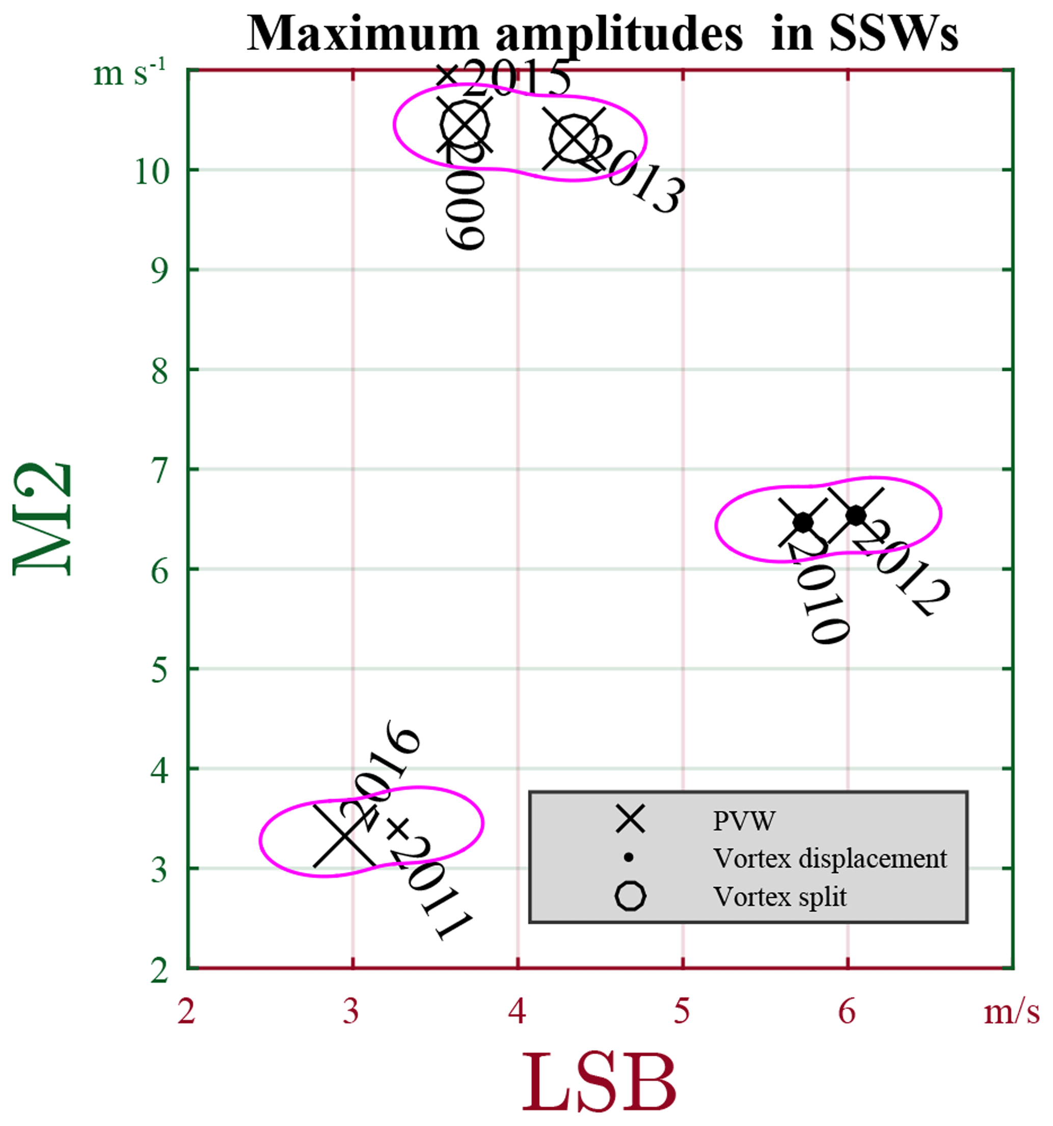
Figure 5Scatterplots of the maximum amplitudes of LSB and M2 during SSWs, read from Fig. 3. The size of the cross is proportional to the PVW strength defined by Zhang et al. (2014). The magenta circles cluster the PVWs into three main groups according to the SSW classification according to the associated polar vortex split or displacement.
We further investigate three clusters in Fig. 5 according to a classification of associated major SSWs (cf. Seviour et al., 2016; Esler and Matthewman, 2011): vortex-split or displacement marked by solid and unfilled black circles, respectively. Clearly, three clusters circled in the magenta lines in Fig. 5 are associated with the SSW classification: (a) the strongest LSB and intermediate M2 occur in vortex-displacement events, (b) the intermediate LSB and strongest M2 occur in vortex-split events, and (c) the weakest M2 and weakest LSB occur mostly in nonmajor SSW events. Here, nonmajor SSW events refer to the minor and final SSWs (cf. Butler et al., 2015, 2017; Limpasuvan et al., 2005). The only exception in this classification is the 2015 event.
The association between the SSW classification and M2 strength is consistent with the conclusion drawn from more SSW events using equatorial magnetic field observations (e.g., Siddiqui et al., 2018). Here, our multi-SMR-jointed analysis allows us to separate LSB and M2 components that share the same period. Our results imply that LSB has contaminated previous M2 estimations based on single-site observations, particularly during vortex-displacement SSWs. The association between the vortex displacement SSW and M2 implies an alternative explanation for the LSB signatures at T=12.4 h with m=1. Although it has never been proposed in existing literature, the LSB signature might be, according to the resonant condition, a secondary wave of the nonlinear interaction between stationary PW with zonal wave number 1 structure (sPW1) and M2. Although our analysis is not sufficient to exclude the possibility of the sPW1–M2 interaction, evidence from case studies was reported to only support the PW–SW2 interaction, including the triple co-occurrence and triple coherency of the three involved waves, and the accompany or occurrence of the USB (e.g., He et al., 2017). On the contrary, against the sPW1–M2 interaction is the fact that the LSB signature was observed without co-occurrence of significant M2 (e.g., He et al., 2018b). Accordingly, throughout the current work, we explain the LSB signature as a secondary wave of the PW–SW2 interaction.
In the current section, we change our focus to the seasonal climatology of the identified six waves. Similar to Fig. 4a–f showing the SSW CA with respect to PVW, Fig. 4g–l display the CA results with respect to the start of the calendar year. Figure 4g–l exhibit similarities with Fig. 4a–f, e.g., similar vertical and temporal extensions of the primary peaks. The similarities are not surprising since the time epochs are close to each other: PVWs always occurred in winter near the start of the new year. In comparison with the SSW CA results, in the calendar CA the primary peaks of LSB, USB, and M2 (Fig. 4g–i) are slightly smeared out. In contrast, the peaks of the solar tides (SW1, SW2, and SW3 in Fig. 4j, k, and l) have not been smeared out in the calendar CA, the peaks of SW2 and SW3 are even sharper and stronger. These results suggest that the temporal variations of LSB, USB, and M2 are characterized more by their responses to SSWs than by their seasonal variations, whereas those of the solar tides are characterized more by the seasonal variations.
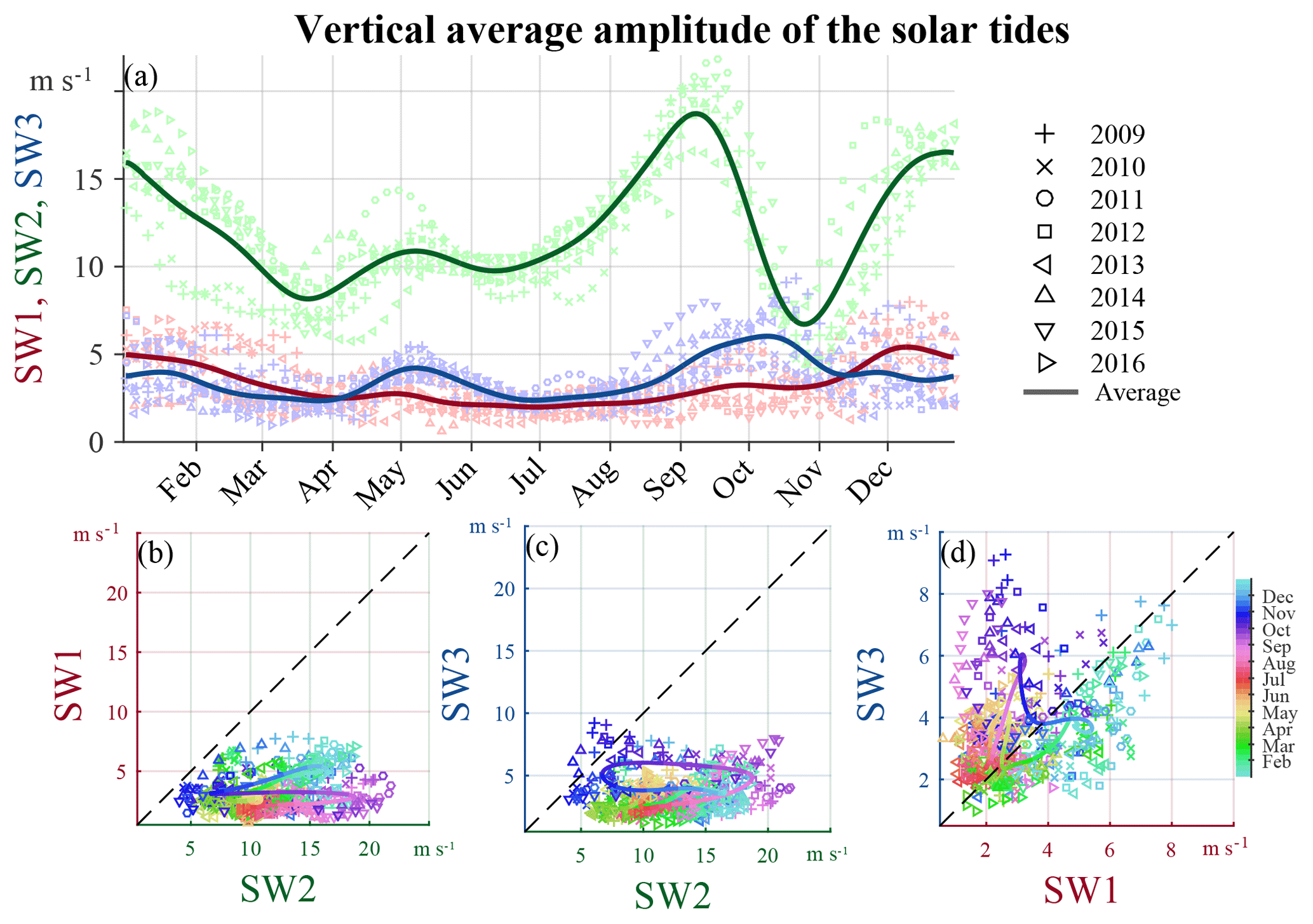
Figure 6(a) Vertical average amplitudes of SW1, SW2, and SW3 scattered as a function of date. (b, c, d) Scatterplot between the vertical average amplitudes of SW2 vs. SW1, SW2 vs. SW3, and SW1 vs. SW3. In each panel, each point corresponds to a 5 d interval in Fig. 3; and the solid colored line represents the multi-year average.
5.1 Comparison to previous studies
In the amplitude plots shown in Figs. 4j–l and 3d–f the vertical variations are characterized by larger amplitudes at higher altitudes. MLT waves are often excited in and propagated from the stratosphere or troposphere. The upward propagating waves amplify exponentially with increasing altitude as the air density decreases and then eventually dissipate. Such a simple vertical structure is associated with the fact that in Fig. 3 the temporal variations, both enhancements and weakenings, typically extend into broad altitude ranges. We vertically average the amplitudes shown in Fig. 3d–f for an one-dimensional representation, and display the average as a function of the DoY in Fig. 6a. The averaged components are shown as a scatterplot in Fig. 6b, c, and d, against each other, i.e., for SW1 vs. SW2, SW3 vs. SW2, and SW3 vs. SW1. The most salient feature of the scatters is that SW2 is almost always the dominant component, except in late October when SW3 is comparable to SW2. The scatters are further averaged seasonally displayed as the solid red, green, and blue lines, summarizing the main seasonal variations of SW1, SW2, and SW3. SW2 is characterized by two comparable peaks in September and in December and steep decreases in September–October and March–April (DoY 250–300 and 0–80), which is consistent with the seasonal variation of the 12.0 h harmonic amplitude (S2) observed from single-radar analyses (as used in, e.g., Conte et al., 2018), although the SW1 and SW3 are not negligible in comparison with SW2. SW1 is characterized by a single peak appearing in winter and a minimum in summer, which are largely consistent with thermospheric seasonal variation of SW1 at 50∘ N according to CHAMP observations (Fig. 12, in Oberheide et al., 2011). SW3 is characterized by two peaks in earlier May and October (around DoY 130 and 280). Similar annual dual peaks of SW3 were observed from SABER measurements (Fig. 2.7 in Hartwell, 1994) and also obtained at 50∘ N at 88 km altitude from the 3 years (2006–2008) of simulated data from the Canadian Middle Atmosphere Model Data Assimilation System (Figs. 6b and 10c in Xu et al., 2012). Interestingly, in Fig. 6a, d, the relative importance of SW1 and SW3 switches around early April and November (DoY 90 and 310): in summer SW3 is stronger than SW1, but SW1 is stronger in winter. These seasonal variations might be associated with the climatology of the background mean wind (e.g., Laskar et al., 2016; Conte et al., 2017).

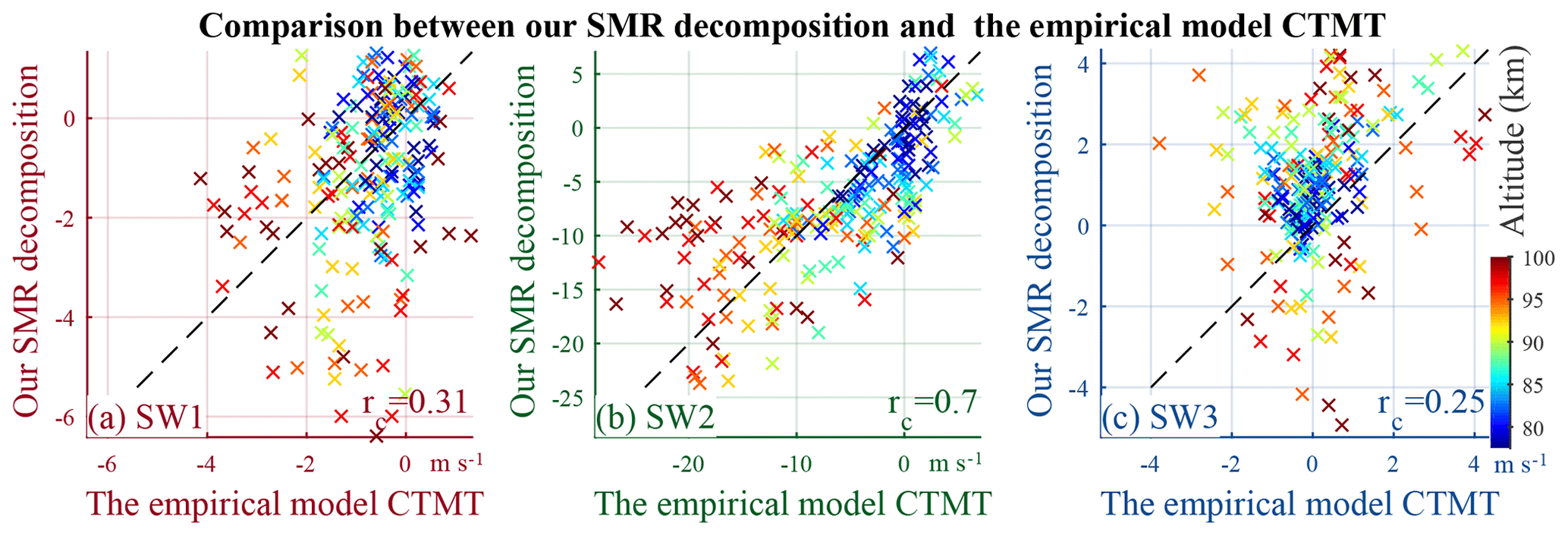
Figure 7(a–c) Same plots as Figs. 4j, k, and l but for complex amplitude of SW1, SW2, and SW3, with their phases shown in (d)–(f). (g–l) Similar plots to (a)–(f) but according to the climatological tidal model of the thermosphere (CTMT) derived from SABER and TIDI observations (Oberheide et al., 2011).
In comparison with some previous studies, the amplitudes in Fig. 3 appear to be weaker (e.g., Jacobi, 2012) for at least three potential reasons. First, based on single-site observations, most existing studies did not separate waves with different wave numbers but had to explain the total oscillations at 12 or 12.4 h as approximations of SW2 or M2 (e.g., Chau et al., 2015). Second, most existing studies used windowing functions much narrower than ours, resulting in broader passbands and capturing more energy (e.g., Chau et al., 2015; Forbes and Zhang, 2012). Third, some studies present the amplitude of total wind including both zonal and meridional (e.g., Chau et al., 2015; Conte et al., 2017), while here we focus only on the zonal component. For a quantitative comparison, in the next section, we present a comparison with an independent empirical tidal model, CTMT.
5.2 A comparison with an empirical model
Figure 7a–f present a composite analysis in the same manner as in Fig. 4j–l but for the amplitude of complex average, . The similarities between Figs. 4j–l and 7a–c indicate that the phases of solar tides are consistent from year to year.
For an independent quantitative comparison, we present the seasonal variation of the solar tides according to CTMT (Oberheide et al., 2011), in Fig. 7g–l. The CTMT results exhibit some consistency with our results, especially on SW2. SW2 in Fig. 7h maximizes during August–September and December–January, and in between these periods there is a minimum. The vertical gradient is steeper during the August–September maximum than during December–January.
These features are similar to those in Fig. 7b. However, in the CTMT results, the maxima, or the minimum can hardly be observed (Fig. 7h). These morphological discrepancies might arise from the low temporal resolution of the model. The effective resolution is about 2 months, during which the satellite observations used for the model cover the whole local time once. In contrast, the September maximum and the minimum are narrower than 2 months; therefore they might be smeared out. In the case of phase, our result in Fig. 7e also exhibits similarities to the CTMT results in Fig. 7k.
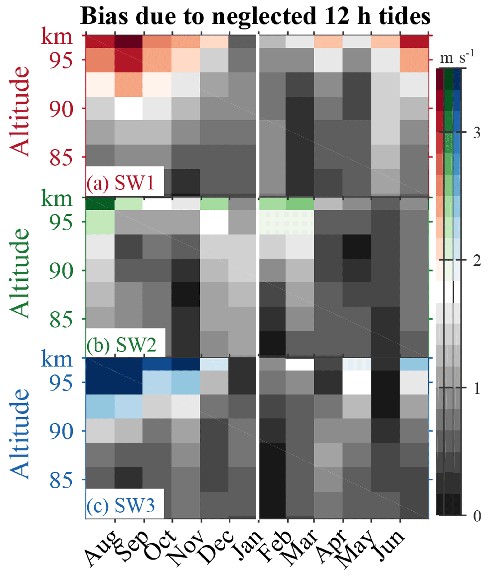
Figure 9The bias of our tidal estimation due to the existence of neglected 12 h tides (including SE3, SE2, SE1, S0, and SW4) predicted by CTMT (Oberheide et al., 2011).
SW3 is compared in Fig. 7c, f, i, and l, from which similarities in both amplitude and phase occur mainly in fall. Although SW3 in the CTMT results also exhibits a second maximum, it occurs during February–March, up to 2 months before the second annual peak in early May from our results (see Figs. 7c and 6a). This difference might be associated with the seasonally uneven sampling of observations used for the model: the satellite takes 2 months to cover all local time sectors. In the case of SW1, major discrepancies are found in both amplitudes and phases. For instance, the December maximum in our results (Fig. 7a) could not be found in the CTMT (Fig. 7g).
These qualitative findings are supported quantitatively by Fig. 8a, b, and c, where the in-phase and quadrature components of our estimations vs. the model are shown as scatterplots for SW1, SW2, and SW3. The highest correlation coefficient is observed in SW2. Since the temporal and vertical resolutions of our results are higher than the CTMT, we smear our results down to the resolutions of CTMT and calculate the correlation coefficients again, yielding correlations coefficients slightly higher than those in Fig. 8 by up to 0.01 (not shown). The correlations are not high overall, reflecting mainly the different assumptions used by the two approaches. Our approaches assume that the meridian tidal variation among our SMRs is negligible, whereas CTMT, as well as any other tidal analyses using single-satellite approaches, assumes the tides are static in the data-binning window. Evaluating these assumptions comparatively entails an independent model with high resolutions in both time and space. Besides, our results might be contaminated by the neglected tides, which is quantified in the next section, whereas the CTMT tidal components might be contaminated by aliasing from waves with similar periods, e.g., the secondary waves and M2.
5.3 Bias of our estimation due to the existence of neglected solar tidal components
For estimating the solar tides and as explained in Sect. 2.2, in our approach we assume that our targeting components, i.e., SW1, SW2, and SW3, are the dominant components at 12.0 h. This assumption might be too strong given that other neglected semidiurnal tidal components have also been reported (e.g., Oberheide et al., 2011; He et al., 2011). The current section quantifies the bias due to the existence of other neglected components according to CTMT.
Arrange Eq. (1) into two parts, namely the targeting components with amplitudes and the neglected components with :
Multiply , resulting in
Here, the term on the left is the estimated amplitude of the targeting components, while the first term on the right is the corresponding real amplitude. Therefore, their difference, i.e., the second term on the right, corresponds to the bias due to the neglected tidal components. According to CTMT, we estimate the bias and display its absolute value in Fig. 9. Contributing to the bias are semidiurnal components SE3, SE2, SE1, S0, and SW4. Overall, the bias is below 2 m s−1 but above 90 km in summer, which suggests our main conclusions in previous sections are not affected by our assumption that SW1, SW2, and SW3 are the dominant components. Actually, when determined by the configuration of the SMRs, the matrices of both and are very well conditioned (with condition numbers of 1.6 and 2.4), suggesting our estimations are not sensitively affected by the errors in both the wavelet spectra and the neglected semidiurnal components.
Our comparison from the previous section has stressed the additional information that our results bring, specifically, those on SW1 and SW3. In future efforts, we plan to add more ground-based observations and try to combine them with satellite-based wind and temperature observations (cf. Zhou et al., 2018) to improve our understanding of mesospheric tides. Although the current work focuses on the near-12 h waves at midlatitudes, our joint data set analysis approach could be extended to other periods, e.g., diurnal or terdiurnal tides.
By combining mesospheric zonal wind observations collected by five midlatitude SMRs from three longitudinal sectors, we develop an approach to statistically investigate six waves at periods close to 12 h, namely three solar tides (SW1, SW2, and SW3), two sidebands of nonlinear modulation of 16 d wave on SW2 (LSB and USB), and a lunar tide (M2). We first filter the observation from each SMR into three narrow frequency bands through a high-frequency-resolved wavelet analysis. Then, in each of the three bands, wavelet spectra from all SMRs are combined to fit the potential waves. The results suggest that the temporal variations of the waves are characterized by responses to SSWs (enhancements of LSB, USB, and M2, and a decrease in SW2) and climatological seasonal variations of the solar tides. Our main results are as follows:
-
Contrary to most extensive previous literature, our results suggest that SW1 and SW3 do not statistically enhance during SSWs. The LSB and USB enhancements have been misinterpreted as SW1 and SW3 signatures, respectively. Meanwhile, the enhancements are associated with a decrease in SW2, which could be explained in terms of the energy exchange through the nonlinear interaction.
-
Both enhancements of LSB and M2 depend on the SSW classification with respect to the polar vortex split or displacement. M2 enhancement is stronger during vortex split SSWs than that during the vortex displacement, whereas LSB is the other way around. Overall, M2 is stronger than LSB, except during the vortex-displacement SSW when they are comparable, implicating that LSB might contaminate the existing M2 estimations based on single-site observations.
-
The seasonal variations of solar tides are in reasonable agreement with existing observational studies: SW2 is the dominant component, which maximizes around September and December followed by two minima; SW1 maximizes in winter, and SW3 maximizes in fall and spring. In October, when SW3 is at its annual maximum and SW2 is at a minimum, their strengths are comparable to each other. These results suggest that the 12.0 h harmonic amplitude from single-radar analyses is dominated by SW2 for most of the seasons except in October.
Our main results, namely the complex amplitudes of the six waves as a function of time and altitude, are shared at ftp://ftp.iap-kborn.de/data-in-publications/HeACP2018/ (last access: 19 December 2018). The SMR data from Mohe and Beijing are provided by BNOSE (Beijing National Observatory of Space Environment), IGGCAS (Institute of Geology and Geophysics, Chinese Academy of Sciences) through the Data Center for Geophysics, National Earth System Science Data Sharing Infrastructure (http://wdc.geophys.cn, last access: 3 March 2017). The model CTMT (Climatological Tidal Model of the Thermosphere) is available at http://globaldynamics.sites.clemson.edu/articles/ctmt.html (last access: 28 September 2018).
The conceptualization was done by MH and JLC, the methodology was formulated by MH, the software was developed by MH, the original draft was written by MH, the manuscript was reviewed and edited by MH and JLC, and funding was acquired by JLC.
The authors declare that they have no conflict of interest.
The authors appreciate the suggestions from Weixing Wan of jointly analyzing
SMR observations from different longitudinal sectors, the discussions with
Peter Hoffman on the tidal climatologies, and the discussions with Nick
Pedatella and Jens Oberheider on the error estimation. We thank Guozhu Li for
operating the SMRs at Mohe and Beijing, Christoph Jacobi for the data from
Collm SMR, and Peter Brown for the CMOR SMR data. We are also grateful to
Gunter Stober for processing the hourly wind from SMRs. This study is
partially supported by the WATILA project (SAW-2-15-IAP-5 383) and by the
Deutsche Forschungsgemeinschaft (DFG, German Research Foundation) under SPP
1788 (DynamicEarth) project CH 1482/1-1 (DYNAMITE).
The publication of this article was funded by the
Open Access Fund of the Leibniz Association.
This paper was edited by Thomas von Clarmann and reviewed by two anonymous referees.
Ahlquist, J. E.: Normal-Mode Global Rossby Waves. Theory and Observations, J. Atmos. Sci., 39, 193–202, https://doi.org/10.1175/1520-0469(1982)039<0193:NMGRWT>2.0.CO;2, 1982. a
Angelats I Coll, M. and Forbes, J. M.: Nonlinear interactions in the upper atmosphere: The s=1 and 5=3 nonmigrating semidiurnal tides, J. Geophys. Res.-Space, 107, 1–18, https://doi.org/10.1029/2001JA900179, 2002. a, b
Azeem, S. M., Killeen, T. L., Johnson, R. M., Wu, Q., and Gell, D. A.: Space-time analysis of TIMED Doppler Interferometer (TIDI) measurements, Geophys. Res. Lett., 27, 3297–3300, https://doi.org/10.1029/1999GL011289, 2000. a
Baumgaertner, A. J., Jarvis, M. J., McDonald, A. J., and Fraser, G. J.: Observations of the wavenumber 1 and 2 components of the semi-diurnal tide over Antarctica, J. Atmos. Sol.-Terr. Phys., 68, 1195–1214, https://doi.org/10.1016/j.jastp.2006.03.001, 2006. a, b, c
Butler, A. H., Seidel, D. J., Hardiman, S. C., Butchart, N., Birner, T., and Match, A.: Defining Sudden Stratospheric Warmings, B. Am. Meteorol. Soc., 96, 1913–1928, https://doi.org/10.1175/BAMS-D-13-00173.1, 2015. a
Butler, A. H., Sjoberg, J. P., Seidel, D. J., and Rosenlof, K. H.: A sudden stratospheric warming compendium, Earth Syst. Sci. Data, 9, 63–76, https://doi.org/10.5194/essd-9-63-2017, 2017. a
Chapman, S. and Lindzen, R. S.: Atmospheric Tides: Thermal and Gravitational: Nomenclature, Notation and New Results, https://doi.org/10.1175/1520-0469(1970)027<0707:ATTAGN>2.0.CO;2, 1970. a, b
Chau, J. L., Hoffmann, P., Pedatella, N. M., Matthias, V., and Stober, G.: Upper mesospheric lunar tides over middle and high latitudes during sudden stratospheric warming events, J. Geophys. Res.-Space, 120, 3084–3096, https://doi.org/10.1002/2015JA020998, 2015. a, b, c, d, e, f, g
Chree, C.: Some Phenomena of Sunspots and of Terrestrial Magnetism, Part II, Philos. Trans. R. Soc. London. Ser. A, 213, 245–277, https://doi.org/10.1098/rsta.1913.0003, 1914. a
Conte, J. F., Chau, J. L., Stober, G., Pedatella, N., Maute, A., Hoffmann, P., Janches, D., Fritts, D., and Murphy, D. J.: Climatology of semidiurnal lunar and solar tides at middle and high latitudes: Interhemispheric comparison, J. Geophys. Res.-Space, 122, 7750–7760, https://doi.org/10.1002/2017JA024396, 2017. a, b
Conte, J. F., Chau, J. L., Laskar, F. I., Stober, G., Schmidt, H., and Brown, P.: Semidiurnal solar tide differences between fall and spring transition times in the Northern Hemisphere, Ann. Geophys., 36, 999–1008, https://doi.org/10.5194/angeo-36-999-2018, 2018. a
Day, K. A. and Mitchell, N. J.: The 16-day wave in the Arctic and Antarctic mesosphere and lower thermosphere, Atmos. Chem. Phys., 10, 1461–1472, https://doi.org/10.5194/acp-10-1461-2010, 2010. a
Esler, J. G. and Matthewman, N. J.: Stratospheric Sudden Warmings as Self-Tuning Resonances, Part II: Vortex Displacement Events, J. Atmos. Sci., 68, 2505–2523, https://doi.org/10.1175/JAS-D-11-08.1, 2011. a
Fejer, B. G., Olson, M. E., Chau, J. L., Stolle, C., Luehr, H., Goncharenko, L. P., Yumoto, K., and Nagatsuma, T.: Lunar-dependent equatorial ionospheric electrodynamic effects during sudden stratospheric warmings, J. Geophys. Res.-Space, 115, 1–9, https://doi.org/10.1029/2010JA015273, 2010. a
Fejer, B. G., Tracy, B. D., Olson, M. E., and Chau, J. L.: Enhanced lunar semidiurnal equatorial vertical plasma drifts during sudden stratospheric warmings, Geophys. Res. Lett., 38, 7271, https://doi.org/10.1029/2011GL049788, 2011. a
Forbes, J. M. and Zhang, X.: Lunar tide amplification during the January 2009 stratosphere warming event: Observations and theory, J. Geophys. Res.-Space, 117, 1–13, https://doi.org/10.1029/2012JA017963, 2012. a, b
Goncharenko, L. and Zhang, S. R.: Ionospheric signatures of sudden stratospheric warming: Ion temperature at middle latitude, Geophys. Res. Lett., 35, 4–7, https://doi.org/10.1029/2008GL035684, 2008. a
Goncharenko, L., Chau, J. L., Condor, P., Coster, A., and Benkevitch, L.: Ionospheric effects of sudden stratospheric warming during moderate-to-high solar activity: Case study of January 2013, Geophys. Res. Lett., 40, 4982–4986, https://doi.org/10.1002/grl.50980, 2013. a
Grossmann, A., Kronland-Martinet, R., and Morlet, J.: Reading and Understanding Continuous Wavelet Transforms, in: Wavelets, edited by: Combes, J.-M., Grossmann, A., and Tchamitchian, P., 2–20, Springer, Berlin, Heidelberg, 1990. a
Hartwell, F. P.: Wiring methods for patient care areas, vol. 93, https://doi.org/10.1007/978-94-007-0326-1, 1994. a
He, M., Liu, L., Wan, W., and Wei, Y.: Strong evidence for couplings between the ionospheric wave-4 structure and atmospheric tides, Geophys. Res. Lett., 38, L14101, https://doi.org/10.1029/2011GL047855, 2011. a
He, M., Chau, J. L., Stober, G., Hall, C. M., Tsutsumi, M., and Hoffmann, P.: Application of Manley-Rowe relation in analyzing nonlinear interactions between planetary waves and the solar semidiurnal tide during 2009 sudden stratospheric warming event, J. Geophys. Res.-Space, 122, 10783–10795, https://doi.org/10.1002/2017JA024630, 2017. a, b, c, d, e, f, g, h, i
He, M., Chau, J. L., Hall, C., Tsutsumi, M., Meek, C., and Hoffmann, P.: The 16-day planetary wave triggers the SW1-tidal-like signatures during 2009 sudden stratospheric warming, Geophys. Res. Lett., 45, 12631–12638, https://doi.org/10.1029/2018GL079798, 2018a. a, b, c, d, e, f, g, h
He, M., Chau, J. L., Stober, G., Li, G., Ning, B., and Hoffmann, P.: Relations Between Semidiurnal Tidal Variants Through Diagnosing the Zonal Wavenumber Using a Phase Differencing Technique Based on Two Ground-Based Detectors, J. Geophys. Res.-Atmos., 123, 4015–4026, https://doi.org/10.1002/2018JD028400, 2018b. a, b, c, d, e, f, g
Hocking, W., Fuller, B., and Vandepeer, B.: Real-time determination of meteor-related parameters utilizing modern digital technology, J. Atmos. Sol.-Terr. Phys., 63, 155–169, https://doi.org/10.1016/S1364-6826(00)00138-3, 2001. a
Jacobi, C.: 6 year mean prevailing winds and tides measured by VHF meteor radar over Collm (51.3∘ N, 13.0∘ E), J. Atmos. Sol.-Terr. Phys., 78–79, 8–18, https://doi.org/10.1016/j.jastp.2011.04.010, 2012. a, b
Jones, J., Brown, P., Ellis, K., Webster, A., Campbell-Brown, M., Krzemenski, Z., and Weryk, R.: The Canadian Meteor Orbit Radar: system overview and preliminary results, Planet. Space Sci., 53, 413–421, https://doi.org/10.1016/j.pss.2004.11.002, 2005. a, b
Laskar, F. I., Chau, J. L., Stober, G., Hoffmann, P., Hall, C. M., and Tsutsumi, M.: Quasi-biennial oscillation modulation of the middle- and high-latitude mesospheric semidiurnal tides during August–September, J. Geophys. Res.-Space, 121, 4869–4879, https://doi.org/10.1002/2015JA022065, 2016. a
Limpasuvan, V., Hartmann, D. L., Thompson, D. W., Jeev, K., and Yung, Y. L.: Stratosphere-troposphere evolution during polar vortex intensification, J. Geophys. Res.-Atmos., 110, 1–15, https://doi.org/10.1029/2005JD006302, 2005. a
Liu, H. L., Wang, W., Richmond, A. D., and Roble, R. G.: Ionospheric variability due to planetary waves and tides for solar minimum conditions, J. Geophys. Res.-Space, 115, A00G01, https://doi.org/10.1029/2009JA015188, 2010. a, b
Liu, L., Liu, H., Chen, Y., Le, H., Sun, Y.-Y., Ning, B., Hu, L., and Wan, W.: Variations of the meteor echo heights at Beijing and Mohe, China, J. Geophys. Res.-Space, 122, 1117–1127, https://doi.org/10.1002/2016JA023448, 2016. a
Liu, L., Liu, H., Le, H., Chen, Y., Sun, Y. Y., Ning, B., Hu, L., Wan, W., Li, N., and Xiong, J.: Mesospheric temperatures estimated from the meteor radar observations at Mohe, China, J. Geophys. Res.-Space, 122, 2249–2259, https://doi.org/10.1002/2016JA023776, 2017. a
Longuet-Higgins, M. S.: The Eigenfunctions of Laplace's Tidal Equations over a Sphere, Philos. Trans. R. Soc. A, 262, 511–607, https://doi.org/10.1098/rsta.1968.0003, 1968. a
Luo, Y., Manson, A. H., Meek, C. E., Meyer, C. K., Burrage, M. D., Fritts, D. C., Hall, C. M., Hocking, W. K., MacDougall, J., Riggin, D. M., and Vincent, R. A.: The 16-day planetary waves: multi-MF radar observations from the arctic to equator and comparisons with the HRDI measurements and the GSWM modelling results, Ann. Geophys., 20, 691–709, https://doi.org/10.5194/angeo-20-691-2002, 2002. a
Madden, R. A.: Large-scale, free Rossby waves in the atmosphere – An update, Tellus A, 59, 571–590, https://doi.org/10.1111/j.1600-0870.2007.00257.x, 2007. a
Manson, A. H., Meek, C. E., Chshyolkova, T., Xu, X., Aso, T., Drummond, J. R., Hall, C. M., Hocking, W. K., Jacobi, Ch., Tsutsumi, M., and Ward, W. E.: Arctic tidal characteristics at Eureka (80∘ N, 86∘ W) and Svalbard (78∘ N, 16∘ E) for 2006/07: seasonal and longitudinal variations, migrating and non-migrating tides, Ann. Geophys., 27, 1153–1173, https://doi.org/10.5194/angeo-27-1153-2009, 2009. a, b
Murphy, D. J.: Variations in the phase of the semidiurnal tide over Davis, Antarctica, J. Atmos. Sol.-Terr. Phys., 64, 1069–1081, https://doi.org/10.1016/S1364-6826(02)00058-5, 2002. a
Murphy, D. J.: Observations of a nonmigrating component of the semidiurnal tide over Antarctica, J. Geophys. Res., 108, 4241, https://doi.org/10.1029/2002JD003077, 2003. a, b, c
Murphy, D. J., Forbes, J. M., Walterscheid, R. L., Hagan, M. E., Avery, S. K., Aso, T., Fraser, G. J., Fritts, D. C., Jarvis, M. J., McDonald, A. J., Riggin, D. M., Tsutsumi, M., and Vincent, R. A.: A climatology of tides in the antarctic mesosphere and lower thermosphere, J. Geophys. Res.-Atmos., 111, 1–17, https://doi.org/10.1029/2005JD006803, 2006. a
Murphy, D. J., Aso, T., Fritts, D. C., Hibbins, R. E., McDonald, A. J., Riggin, D. M., Tsutsumi, M., and Vincent, R. A.: Source regions for antarctic MLT non-migrating semidiurnal tides, Geophys. Res. Lett., 36, 1–5, https://doi.org/10.1029/2008GL037064, 2009. a
Oberheide, J., Hagan, M. E., and Roble, R. G.: Tidal signatures and aliasing in temperature data from slowly precessing satellites, J. Geophys. Res.-Space, 108, 1055, https://doi.org/10.1029/2002JA009585, 2002. a
Oberheide, J., Forbes, J. M., Zhang, X., and Bruinsma, S. L.: Climatology of upward propagating diurnal and semidiurnal tides in the thermosphere, J. Geophys. Res.-Space, 116, A11306, https://doi.org/10.1029/2011JA016784, 2011. a, b, c, d, e, f, g, h
Pancheva, D. and Mukhtarov, P.: Global response of the ionosphere to atmospheric tides forced from below: Recent progress based on satellite measurements: Esponse of the ionosphere, vol. 168, https://doi.org/10.1007/s11214-011-9837-1, 2012. a
Pancheva, D., Mukhtarov, P., Mitchell, N. J., Merzlyakov, E., Smith, A. K., Andonov, B., Singer, W., Hocking, W., Meek, C., Manson, A., and Murayama, Y.: Planetary waves in coupling the stratosphere and mesosphere during the major stratospheric warming in 2003/2004, J. Geophys. Res.-Atmos., 113, 1–22, https://doi.org/10.1029/2007JD009011, 2008. a
Paschmann, G. and Daly, P. W.: Analysis methods for multi-spacecraft data, ESA Publications Division, Noordwijk, 1998. a
Pedatella, N. M. and Forbes, J. M.: Evidence for stratosphere sudden warming-ionosphere coupling due to vertically propagating tides, Geophys. Res. Lett., 37, L11104, https://doi.org/10.1029/2010GL043560, 2010. a
Pedatella, N. M. and Liu, H. L.: The influence of atmospheric tide and planetary wave variability during sudden stratosphere warmings on the low latitude ionosphere, J. Geophys. Res.-Space, 118, 5333–5347, https://doi.org/10.1002/jgra.50492, 2013. a
Pedatella, N. M., Liu, H. L., Richmond, A. D., Maute, A., and Fang, T. W.: Simulations of solar and lunar tidal variability in the mesosphere and lower thermosphere during sudden stratosphere warmings and their influence on the low-latitude ionosphere, J. Geophys. Res.-Space, 117, A08326, https://doi.org/10.1029/2012JA017858, 2012. a
Salby, M. L.: Sampling Theory for Asynoptic Satellite Observations, Part I: Space-Time Spectra, Resolution, and Aliasing, J. Atmos. Sci., 39, 2577–2600, https://doi.org/10.1175/1520-0469(1982)039<2577:STFASO>2.0.CO;2, 1982a. a
Salby, M. L.: Sampling Theory for Asynoptic Satellite Observations, Part I: Space-Time Spectra, Resolution, and Aliasing, J. Atmos. Sci., 39, 2577–2600, https://doi.org/10.1175/1520-0469(1982)039<2577:STFASO>2.0.CO;2, 1982b. a
Salby, M. L.: Transient disturbances in the stratosphere: implications for theory and observing systems, J. Atmos.-Terr. Phys., 46, 1009–1047, https://doi.org/10.1016/0021-9169(84)90007-2, 1984. a
Seviour, W. J., Gray, L. J., and Mitchell, D. M.: Stratospheric polar vortex splits and displacements in the high-top CMIP5 climate models, J. Geophys. Res., 121, 1400–1413, https://doi.org/10.1002/2015JD024178, 2016. a
Siddiqui, T. A., Yamazaki, Y., Stolle, C., Lühr, H., Matzka, J., Maute, A., and Pedatella, N.: Dependence of Lunar Tide of the Equatorial Electrojet on the Wintertime Polar Vortex, Solar Flux, and QBO, Geophys. Res. Lett., 45, 3801–3810, https://doi.org/10.1029/2018GL077510, 2018. a
Singer, W., Hoffmann, P., Kishore Kumar, G., Mitchell, N. J., and Matthias, V.: Atmospheric Coupling by Gravity Waves: Climatology of Gravity Wave Activity, Mesospheric Turbulence and Their Relations to Solar Activity, 409–427, Springer Netherlands, Dordrecht, https://doi.org/10.1007/978-94-007-4348-9_22, 2013. a
Stening, R. J.: Lunar tide in the equatorial electrojet in relation to stratospheric warmings, J. Geophys. Res.-Space, 116, A12315, https://doi.org/10.1029/2011JA017047, 2011. a
Stober, G., Jacobi, C., Matthias, V., Hoffmann, P., and Gerding, M.: Neutral air density variations during strong planetary wave activity in the mesopause region derived from meteor radar observations, J. Atmos. Sol.-Terr. Phys., 74, 55–63, https://doi.org/10.1016/j.jastp.2011.10.007, 2012. a
Wu, Q. and Nozawa, S.: Mesospheric and thermospheric observations of the January 2010 stratospheric warming event, J. Atmos. Sol.-Terr. Phys., 123, 22–38, https://doi.org/10.1016/j.jastp.2014.11.006, 2015. a
Xu, X., Manson, A. H., Meek, C. E., Riggin, D. M., Jacobi, C., and Drummond, J. R.: Mesospheric wind diurnal tides within the Canadian Middle Atmosphere Model Data Assimilation System, J. Atmos. Sol.-Terr. Phys., 74, 24–43, https://doi.org/10.1016/j.jastp.2011.09.003, 2012. a
Yu, Y., Wan, W., Ning, B., Liu, L., Wang, Z., Hu, L., and Ren, Z.: Tidal wind mapping from observations of a meteor radar chain in December 2011, J. Geophys. Res.-Space, 118, 2321–2332, https://doi.org/10.1029/2012JA017976, 2013. a
Yu, Y., Wan, W., Ren, Z., Xiong, B., Zhang, Y., Hu, L., Ning, B., and Liu, L.: Seasonal variations of MLT tides revealed by a meteor radar chain based on Hough mode decomposition, J. Geophys. Res.-Space, 120, 7030–7048, https://doi.org/10.1002/2015JA021276, 2015. a
Zhang, J. T., Forbes, J. M., Zhang, C. H., Doornbos, E., and Bruinsma, S. L.: Lunar tide contribution to thermosphere weather, Sp. Weather, 12, 538–551, https://doi.org/10.1002/2014SW001079, 2014. a
Zhang, X. and Forbes, J. M.: Lunar tide in the thermosphere and weakening of the northern polar vortex, Geophys. Res. Lett., 41, 8201–8207, https://doi.org/10.1002/2014GL062103, 2014. a
Zhou, X., Wan, W., Yu, Y., Ning, B., Hu, L., and Yue, X.: New Approach to Estimate Tidal Climatology From Ground- and Space-Based Observations, J. Geophys. Res.-Space, 123, 5087–5101, https://doi.org/10.1029/2017JA024967, 2018. a