the Creative Commons Attribution 4.0 License.
the Creative Commons Attribution 4.0 License.
 | 26 Apr 2019
Estimation of hourly land surface heat fluxes over the Tibetan Plateau by the combined use of geostationary and polar-orbiting satellites
Yaoming Ma
Zeyong Hu
Yunfei Fu
Yuanyuan Hu
Xian Wang
Meilin Cheng
Nan Ge
Estimation of land surface heat fluxes is important for energy and water cycle studies, especially on the Tibetan Plateau (TP), where the topography is unique and the land–atmosphere interactions are strong. The land surface heating conditions also directly influence the movement of atmospheric circulation. However, high-temporal-resolution information on the plateau-scale land surface heat fluxes has been lacking for a long time, which significantly limits the understanding of diurnal variations in land–atmosphere interactions. Based on geostationary and polar-orbiting satellite data, the surface energy balance system (SEBS) was used in this paper to derive hourly land surface heat fluxes at a spatial resolution of 10 km. Six stations scattered throughout the TP and equipped for flux tower measurements were used to perform a cross-validation. The results showed good agreement between the derived fluxes and in situ measurements through 3738 validation samples. The root-mean-square errors (RMSEs) for net radiation flux, sensible heat flux, latent heat flux and soil heat flux were 76.63, 60.29, 71.03 and 37.5 W m−2, respectively; the derived results were also found to be superior to the Global Land Data Assimilation System (GLDAS) flux products (with RMSEs for the surface energy balance components of 114.32, 67.77, 75.6 and 40.05 W m−2, respectively). The diurnal and seasonal cycles of the land surface energy balance components were clearly identified, and their spatial distribution was found to be consistent with the heterogeneous land surface conditions and the general hydrometeorological conditions of the TP.
- Article
(7423 KB) - Full-text XML
-
Supplement
(412 KB) - BibTeX
- EndNote


Mass and energy exchanges are constantly carried out between the land surface and the atmosphere above. At the same time, the weather, climate and environmental changes at multiple spatiotemporal scales are greatly influenced by such land–atmosphere exchanges. Land–atmosphere interaction is a popular topic not only in the field of atmospheric research but also in hydrology, geography, ecology and environmental sciences. The impacts of land–atmosphere interactions on weather and climate change have been assessed through surface sensible heat flux, latent heat flux and momentum flux (Seneviratne et al., 2008; Ma et al., 2017). Developing a method to accurately derive surface heat fluxes has always been a primary focus in atmospheric science research.
The Tibetan Plateau (TP), with an average elevation of more than 4000 m, is also called “the Third Pole” and “the World Roof”. The thermal and dynamic effects caused by the TP's high elevation and relief have profound impacts on atmospheric circulation, the Asian monsoon and global climate change (Ye and Gao, 1979; Ma et al., 2006, 2008; Zhong et al., 2011; Zou et al., 2017, 2018). The interactions between TP multispheres, such as the atmosphere, hydrosphere, lithosphere, biosphere and cryosphere, are the drivers of all these changes. The TP is also one of the most sensitive regions in response to global climate change (Liu et al., 2000). In recent years, some studies have argued that the major factor impacting the South Asian monsoon is the insulating effect of the southern mountain edges of the TP, rather than the elevated heating by the TP (Boos and Kuang, 2010, 2013). However, some other studies have proven that the thermal effects of the TP are the main driving force of the South Asian summer monsoon (Wu et al., 2012, 2015). Obviously, opinions differ in understanding the thermal forcing by the TP. One of the most important reasons is that high spatial and temporal resolution data on land–atmosphere interactions, which can be used in different climate models, are still lacking. To study the characteristics of land–atmosphere interactions in the TP, it is necessary to estimate the surface energy heat fluxes with a fine spatial and temporal resolution over the TP.
Traditional surface energy flux measurements are not only expensive but also limited at the point scale, and it is impossible to meet the need for a larger spatial scale with the complex terrain and landscapes of the TP. However, remote sensing provides the possibility of deriving surface heat fluxes at a regional scale (Ma et al., 2002; Zhong et al., 2014). The methods of estimating surface energy flux by remote sensing can be roughly divided into three categories: the empirical (semiempirical) model, theoretical model and data assimilation system. The empirical (semiempirical) model is mainly based on an empirical formula between surface energy fluxes and surface characteristic parameters. The method itself is simple, but its applicability is limited. The basis of the theoretical model is the surface energy balance equation. The physical model mainly includes a single-source model and a double-source model. The single-source model does not distinguish vegetation transpiration and soil evaporation but tends to consider them as a whole (Su, 2002; Jia et al., 2003; Roerink et al., 2000; Bastiaanssen et al., 1998; Allen et al., 2007). The double-source model separates the vegetation canopy from the soil and calculates the soil temperature and canopy temperature. Then, the sensible heat flux and latent heat flux are calculated (Norman et al., 1995; Sánchez et al., 2008). In recent years, the land surface temperature (LST) and vegetation index data retrieved from satellites have been successfully assimilated in the variational data assimilation (VDA) frameworks to estimate surface heat fluxes (Crow and Kustas, 2005; Bateni et al., 2013; Xu et al., 2014; Abdolghafoorian et al., 2017; Xu et al., 2019). This kind of method does not require any empirical or site-specific relationships and can provide temporally continuous surface heat flux estimates from discrete spaceborne LST observations (Xu et al., 2014).
Some studies have been carried out to estimate surface energy fluxes over the TP based on polar-orbiting satellite data. Ma et al. (2003) estimated the surface energy flux of the Coordinated Enhanced Observing Period (CEOP) of the Asia–Australia Monsoon Project (CAMP) on the Tibetan Plateau (CAMP/Tibet) area using NOAA-14 Advanced Very High Resolution Radiometer (AVHRR) data. The results show that the estimated surface energy flux is in good agreement with the in situ measurements. Oku et al. (2007) used the LST derived from the Stretched Visible and Infrared Spin Scan Radiometer (SVISSR) aboard the Geostationary Meteorological Satellite 5 (GMS-5) and other essential parameters from NOAA–AVHRR and ERA-40 to estimate land surface heat fluxes for regions above 4000 m over the TP. However, the coarse resolution of ERA-40 (25 km) and large error of the LST (more than 10 K) introduced large uncertainties into the final results. Ma et al. (2009) estimated the surface characteristic parameters and surface energy flux of the northern TP in summer, winter and spring using a parameterized scheme for Advanced Spaceborne Thermal Emission and Reflection Radiometer (ASTER) satellite data. Chen et al. (2013a) used observations from four sites in the TP to evaluate the results of the surface energy balance system (SEBS) model and optimize the thermodynamic roughness parameterization scheme for the underlying surface of bare soil. Based on Landsat Thematic Mapper/Enhanced Thematic Mapper Plus (TM/ETM+) data, Chen et al. (2013b) derived the surface energy flux of the Mount Everest area by using the enhanced SEBS model (TESEBS), which takes into account the influence of terrain factors on solar radiation, and the SEBS model. The results show that the estimated results from the TESEBS model are superior to those from the SEBS model for high-resolution satellite images.
At present, the estimation of the surface energy flux of the TP is mainly based on polar-orbiting satellite data. Because of the low temporal resolution of the polar-orbiting satellites, time series of land–atmosphere energy and water exchange data with high temporal resolution in the TP have not been retrieved to date, and the effective basic parameters for the climate model cannot yet be provided. In addition, one of the basic characteristics of the atmospheric boundary layer is its diurnal variation, and information on daily variations in surface energy flux is also lacking over the TP.
This paper mainly focused on how to acquire time series of energy flux data with high temporal resolution using a combination of geostationary and polar-orbiting satellite data. First, the surface energy fluxes over the TP were estimated using the SEBS model with inputs from the high-temporal-resolution LST from FengYun-2C (FY-2C) data and other land surface characteristic parameters from polar-orbiting satellite data. Then, the derived land surface heat fluxes were validated by flux tower measurements and were also compared with Global Land Data Assimilation System (GLDAS) flux products. The study area and datasets used in this study are introduced in Sect. 2. The model description is given in Sect. 3, followed by the results and discussion in Sect. 4. The main conclusions are drawn in Sect. 5.
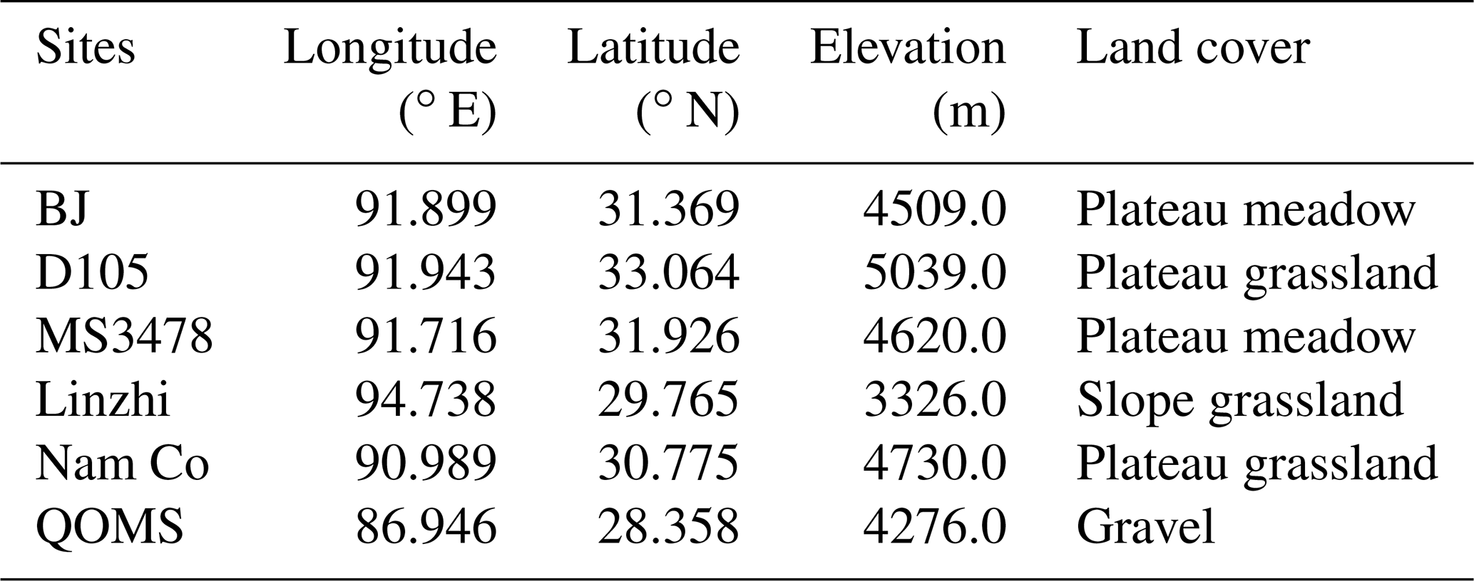
The TP, located in southwest China, has an area of approximately 2.5×10⁶ km2 (Fig. 1) and is the largest plateau in China. With an average elevation of approximately 4000 m, the TP is also the highest plateau in the world, and the high elevation can directly influence the middle and upper layers of the atmosphere. Due to the harsh climate conditions and complex topography of the TP, the meteorological stations in this area are not only sparse but also unevenly distributed. A total of six meteorological stations are used for comparison with model estimates. Although these six stations are not scattered throughout the entire TP, they include several major land cover types (Zhong et al., 2010), and their elevation varies from 3000 to 5000 m (Table 1). These stations are the only stations currently available, and each station is equipped to make four-component radiation measurements, soil moisture and temperature measurements, eddy-covariance measurements, and conventional observation items such as wind speed (u), air temperature (Ta), specific humidity (SH) and air pressure (Ps).
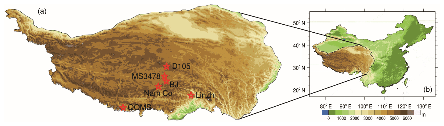
Figure 1Location of the Tibetan Plateau. Panel (b) illustrates the location of the Tibetan Plateau in China. Panel (a) shows the spatial distribution of eddy-covariance stations in the Tibetan Plateau. The pentagrams represent the eddy-covariance stations in the Tibetan Plateau. The legend of the color map indicates the elevation above mean sea level in meters.
Both the geostationary satellite FengYun 2C (FY-2C) and the polar-orbiting satellite SPOT are used to retrieve the essential land surface characteristic parameters. The SVISSR aboard FY-2C is used to derive the hourly LST with a spatial resolution of 5 km, following the algorithms developed by our group (Hu et al., 2018). We should point out here that SVISSR has no infrared channel, which would be needed to derive the normalized difference vegetation index (NDVI), albedo and emissivity. Supposing that these parameters (NDVI, albedo and emissivity) have little variation during a day, the product of the orbiting satellite SPOT is used instead. The spatial resolution for the NDVI, albedo and emissivity is 1 km, with a daily temporal resolution. All the above satellite data with a higher spatial resolution were resampled to match the resolution of the meteorological forcing data (Zou et al., 2018). The time period for all meteorological data and satellite data covers the whole year of 2008.
A forcing dataset developed by the Institute of Tibetan Plateau Research, Chinese Academy of Sciences (ITPCAS), is used as the model input in this study. The dataset has merged the observations from 740 operational stations of the China Meteorological Administration (CMA) with the corresponding Princeton Global Meteorological Forcing Dataset (He, 2010; Yang et al., 2010). The parameters used in this study are downward shortwave radiation (Rswd), downward longwave radiation (Rlwd), wind speed, air temperature, specific humidity and air pressure. All these parameters have a spatial resolution of 10 km and a temporal resolution of 3 h (Table 2). A linear statistical downscaling method was used to derive hourly meteorological forcing data based on original 3 h forcing data and in situ measurements in this study. The general idea is to establish an empirical relationship between each 3 h in situ measurement. Then this relationship is applied to the meteorological forcing data.
Table 2Summary of the input datasets used for calculating land surface heat fluxes.
The GLDAS products are produced by combining satellite and ground-based observations using advanced land surface modeling and data assimilation techniques (Rodell et al., 2004; Zhong et al., 2011). These products have been proven to simulate optimal fields of land surface states and fluxes in near-real time (Rodell et al., 2004). Here, 3 h land surface heat flux products with a spatial resolution of 25 km are selected for comparison with satellite estimates.
Since six stations in Table 1 were not used in the ITPCAS meteorological forcing data, they can be used as independent data to validate the accuracy of the forcing meteorological data. The root-mean-square error (RMSE), mean bias (MB), mean absolute error (MAE) and correlation coefficient (R) are used to make a comparison between the ITPCAS forcing data and in situ meteorological data:
where xi and obsi are the estimation and measurement, respectively. and are the average values of the estimation and measurement, respectively. As shown in Table 3, all six parameters show reasonable accuracy with the in situ measurements, which means that these forcing parameters can be used as model inputs.
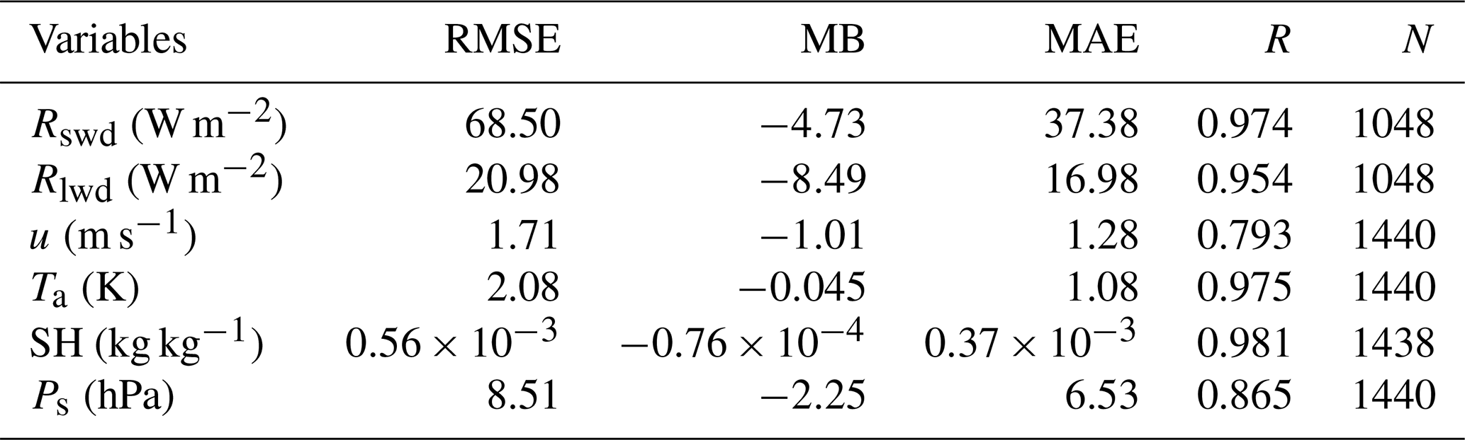
Figure 2 shows the general steps for deriving the land surface heat fluxes in this paper, and the SEBS model is used in this study. A glossary of variables used in determination of land surface heat fluxes can be found in the Supplement (Table S1). Because the surface energy balance has the four components of radiation (Rn), sensible heat flux (Hs), latent heat flux (LE) and soil heat flux (G0), the energy balance equation can be written as
where Rn can be determined by the surface radiation equation as
and where Rswd is the downwelling solar radiation at the land surface. Because there are no infrared channels aboard FY-2C, the NDVI, α and εs are derived from SPOT–VGT data. α is the broadband albedo, which can be derived from the narrowband reflectance of VGT α1, α2, α3 and α4 (Zou et al., 2018). α1, α2, α3 and α4 refer to the reflectance of the blue band, red band, near-infrared band and shortwave infrared band, respectively:
σ in Eq. (6) is the Stefan-Boltzmann constant ( W m−2 K−4). εa and εs are the emissivities of surface air and the land surface, respectively. Ta and Ts are the surface air temperature and LST, respectively. The hourly Ts is derived from split-window algorithms (Hu et al., 2018) based on two thermal bands of FY-2C (Eq. S1–S4 in the Supplement).

Figure 2Flow chart of the flux estimation method to determine the net radiation flux, sensible heat flux and latent heat flux by combining VGT, FY-2C and meteorological forcing data.
The soil heat flux is determined by net radiation flux and vegetation coverage:
where Γs and Γc are ratios of soil heat flux and net radiation flux for bare soil and full vegetation cover, respectively. fc is vegetation coverage and can be derived from the NDVI as follows:
By using the wind speed and air temperature at the reference height, the sensible heat flux, together with the friction velocity and Obukhov stability length, can be derived by solving the following nonlinear Eqs. (11)–(13). Then, the latent heat flux can be estimated by applying Eq. (5):
where L is the Obukhov length, cp is the specific heat at constant pressure, θv is the surface potential virtual air temperature, u* is the friction velocity, k=0.4 is the von Karman constant, g is the acceleration due to gravity, Hs is the sensible heat flux, u is the mean wind speed at reference height z, d0 is the zero-plane displacement height, z0 m is the roughness height for momentum transfer, z0 h is the roughness height for heat transfer, Ψm is the stability correction function for momentum heat transfer, Ψh is the stability correction function for sensible heat transfer, and θ0 and θa are the potential temperatures at the surface and reference height, respectively.
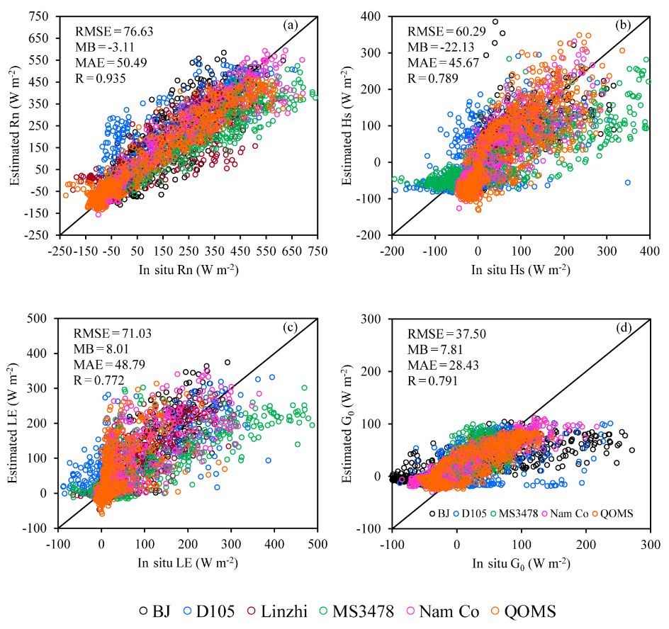
Figure 3Validation of surface heat fluxes estimated by the SEBS model with in situ measurements (a shows net radiation flux, b shows sensible heat flux, c shows latent heat flux and d shows soil heat flux). The legend with different colors indicates the six stations (BJ, D105, Linzhi, MS3478, Nam Co and QOMS) involved in the validation.
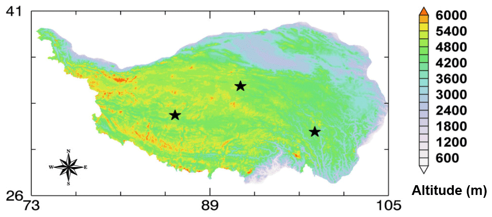
Figure 4Locations of the three sites (marked by pentagrams) used to carry out sensitivity tests of the meteorological forcing input data. The legend of the color map indicates the elevation above mean sea level in meters.
Table 4Comparison of derived flux data product and GLDAS against in situ measurements (units: W m−2).

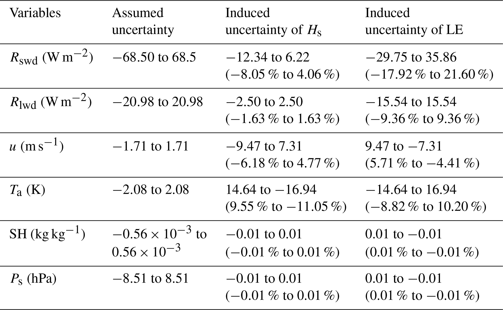
Table 5Uncertainties for each meteorological forcing variable and the induced changes in Hs and LE.
4.1 Validation against in situ flux tower measurements
With the aid of SPOT–VGT and FY-2C–SVISSR data, the surface energy budget components have been estimated using the SEBS model. The accuracy of these estimates needs to be validated before further analyses. A total of six stations over the TP equipped with eddy-covariance measurements were selected for validation (Table 1). These validation stations cover a variety of climates, land cover types and elevations. The in situ flux data have been flagged by steady-state tests and developed conditions tests according to Foken and Wichura (1996) and Foken et al. (2004). Steady conditions mean that all statistical parameters do not vary with time. The flux–variance similarity was used to test the development of turbulent conditions. A data quality of only QA <5 was chosen to make the comparison. As shown in Fig. 3a, b, c and d, the estimates of surface energy budget components show reasonable agreement with the in situ measurements. The RMSEs for the net radiation flux, sensible heat flux, latent heat flux and soil heat flux are 76.63, 60.29, 71.03 and 37.5 W m−2, respectively. The total validation numbers (N) are more than 3837 to make the results much more representative and convincing. It should be noted that some bias exists between the estimated soil heat flux and ground measurements because soil heat flux is parameterized with net radiation flux (Eq. 8). However, soil heat flux and net radiation flux do not have the same diurnal variation shape. The soil heat flux peak values are usually later than the net radiation flux peak values, which was not taken into account in the parameterization. Thus, development of a better parameterization scheme for soil heat flux is needed.
The high-quality, global land surface fields provided by GLDAS support weather and climate prediction, water resources applications, and water cycle investigations. Since the GLDAS data have been widely used, it is meaningful to compare our satellite estimations with these high-quality data to further prove the accuracy of our estimations. To test the robustness of our results, the surface energy budgets obtained from the GLDAS data are selected for comparison with the FY-2C estimations. The comparison shows that the accuracies of the surface energy budgets from the satellite estimation are much higher than those of the GLDAS products (Table 4). The RMSE of the net radiation flux is reduced from 114.32 to 76.63 W m−2, while the values for sensible heat flux, latent heat flux and soil heat flux are reduced from 67.77, 75.6 and 40.05 W m−2 to 60.29, 71.03 and 37.5 W m−2, respectively. Therefore, the new energy budget products not only have a finer spatial (10 km) and temporal resolution (hourly) than traditional polar-orbiting satellite retrievals (e.g., Ma et al., 2006, 2014; Zou et al., 2018) but also possess much higher accuracy than the data assimilation results from GLDAS. Although the SEBS algorithm was used in this study and in Oku et al. (2007; Oku 07 hereinafter), the methods for deriving the land surface characteristic parameters, such as the LST and albedo, are different (Hu et al., 2018; Oku and Ishikawa, 2004; Zou et al., 2018). The higher accuracy and finer spatiotemporal resolution of input forcing data (10 km, 3 h) and land surface characteristic parameters derived from satellites make our results more superior than those of Oku 07. It should also be noted that there is only one station used to perform the validation in Oku 07, while six stations with four major land cover types were used in this study to make the results much more robust. Moreover, our results cover the entire TP, while Oku 07 results only cover the region above 4000 m in the TP.
However, some discrepancies for this new product should be pointed out here, which means improvements are still needed for the current products. The error sources may come from multiple aspects, such as the uncertainties of input forcing data, the accuracy of land surface parameters from satellite retrievals, and some assumptions and simplification in the SEBS model itself. As shown in Fig. 4, three sites located in the northern, western and southeastern parts of the TP were randomly selected to perform the sensitivity analysis. All input meteorological forcing parameters in Table 3 (Rswd, Rlwd, u, Ta, SH and Ps) are selected. The original sensible heat flux and latent heat flux from the SEBS model are used as reference values. The RMSEs of different forcing data are used as perturbations. As shown in Table 5, the sensible heat flux is highly sensitive to Rswd, u and Ta, while the latent heat flux is very sensitive to Rswd, Rlwd and Ta. Both sensible heat flux and latent heat flux are not sensitive to errors of SH and Ps. As Rswd varies from −68.5 to 68.5 W m−2, the induced latent heat flux uncertainty ranges from −29.75 to 35.86 W m−2. Similarly, the sensible heat flux is very sensitive to Ta. When Ta has an uncertainty from −2.08 to 2.08 K, the induced sensible heat flux uncertainty ranges from 14.64 to −16.94 W m−2. Furthermore, the mismatch between in situ measurements at the point level and the scales at the pixel level or grid level may cause some errors. The scale problem is an important issue and should be accounted for. However, this issue goes beyond the scope of this study.
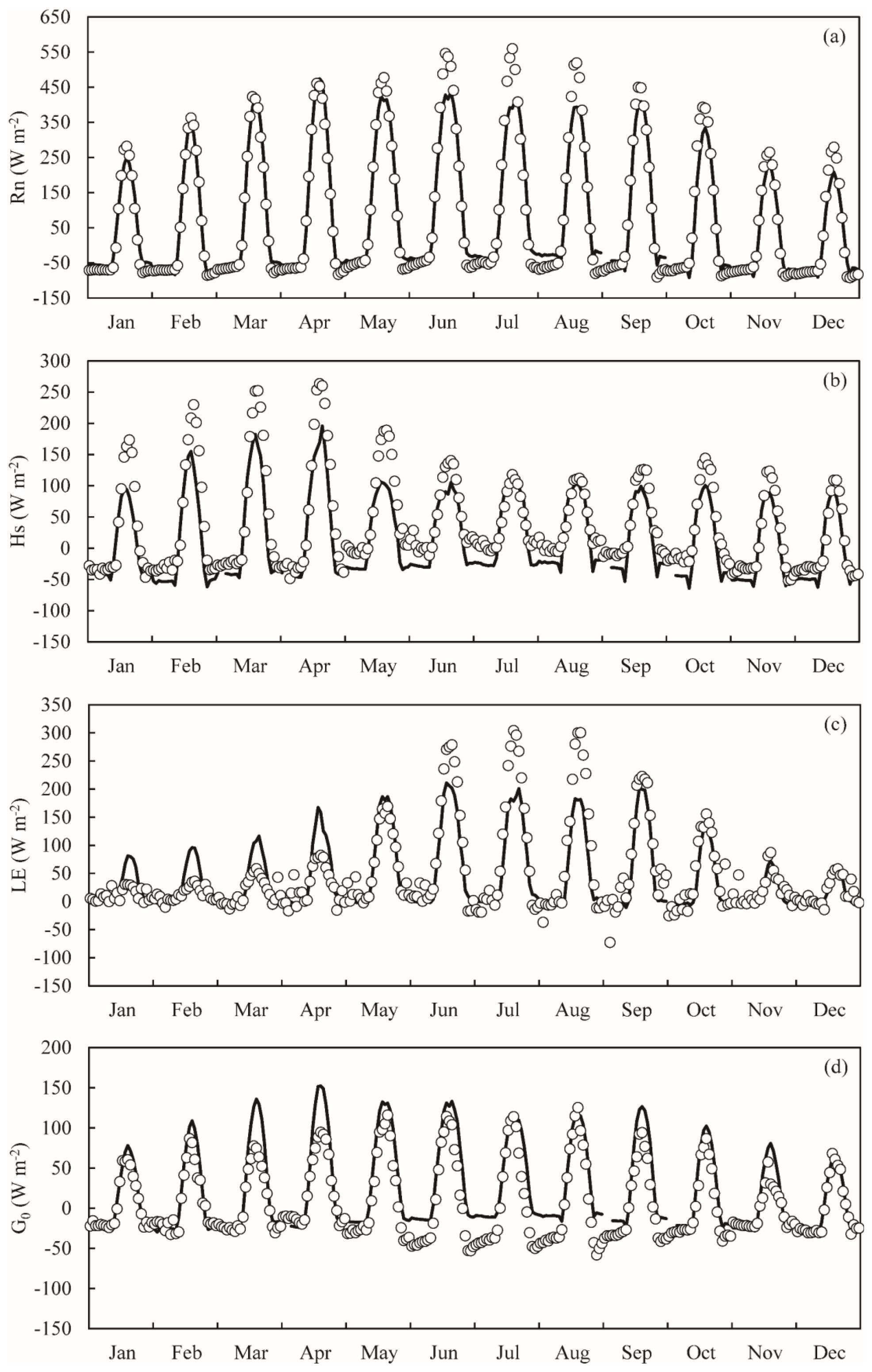
Figure 5Time series of monthly mean diurnal change in surface energy fluxes (units: W m−2) observed by in situ measurements (circle), and those estimated by using the SEBS model (curve) at the BJ station in 2008 (a shows net radiation flux, b shows sensible heat flux, c shows latent heat flux and d shows soil heat flux).
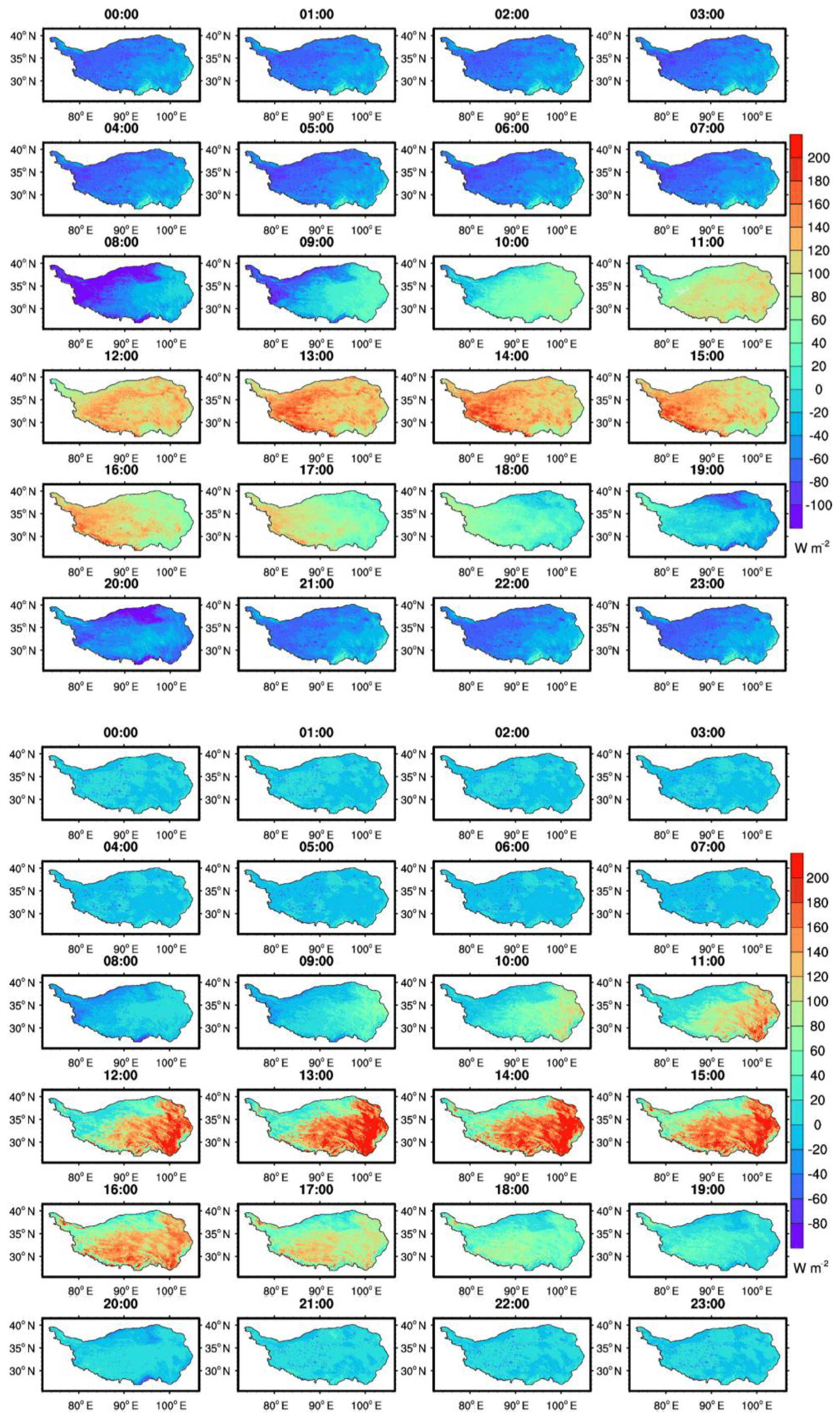
Figure 6Annual mean spatial distribution and diurnal cycle of sensible heat flux (top panels) and latent heat flux (bottom panels) in 2008 over the TP.
4.2 Multitemporal and spatial distribution of surface energy budget components
One-year observation data and satellite estimations at the BJ station were selected for comparison. As shown in Fig. 5, the satellite results can reproduce both the diurnal and seasonal surface flux variations very well. At the daily temporal scale, all the surface heat fluxes increase with sunrise and reach their maximum at midday before decreasing again with sunset. A unique characteristic of the atmospheric boundary layer is its well-known diurnal variations. The diurnal pattern of derived surface heat fluxes is in agreement with the diurnal evolution of the surface atmospheric boundary layer because the surface energy budgets provide a driving force for the surface atmospheric boundary layer. Figure 5 also shows that the flux values are usually positive during the day and become negative during the night. This feature means that the dynamic and thermal contrasts of land and atmosphere are totally different between day and night. The surface heat fluxes during the day are much larger than those during the night. At the seasonal scale, the diurnal mean net radiation flux usually increases from January (15.88 W m−2) to its maximum in June (129.93 W m−2). Then, it decreases again from June to December (2.07 W m−2). The variation trends for sensible heat flux and latent heat flux are quite opposite. Because the TP is greatly influenced by the Asian monsoon system and the vegetation intensity usually increases from May to September (Zhong et al., 2010), the sensible heat flux usually decreases while the latent heat flux usually increases from the premonsoon season to the monsoon season. However, from the monsoon season to the postmonsoon season, the sensible heat flux increases while the latent heat flux decreases. The largest daily average intensity of sensible heat flux was found in April (34.97 W m−2), while that for latent heat flux was found in June (69.09 W m−2). As shown by the surface radiation balance equation (Eq. 6), the downward shortwave radiation is the main incoming energy. A comparison was made between the forcing data and in situ downward radiation at the BJ station. From June to August, the monthly diurnal MB was −4.87 W m−2, which explains why derived net radiation flux was underestimated by the SEBS model from June to August. This phenomenon was also found in the study by Yang et al. (2010). As for the time period from January to May, the underestimation of sensible heat flux was mainly caused by the negative bias of the land–atmosphere air temperature difference. The MB for the land–atmosphere difference could be −5.69 K from January to May. As there is a complementary relationship between sensible heat flux and latent heat flux, the corresponding latent heat flux tends to be overestimated.
A clear diurnal variation in hourly sensible heat flux and latent heat flux maps over the entire TP is shown in Fig. 6. Similar to the diurnal variations in net radiation flux, the amplitude of the sensible heat flux is relatively small before sunrise. Then, the sensible heat flux increases quickly until it reaches its maximum at approximately 14:00 LT (local standard time). After this time, sensible heat flux decreases gradually and tends to be smooth at night. The spatial distribution of sensible heat flux is somewhat complicated. In general, because of the sparse vegetation coverage and limited soil moisture in the western TP, the sensible heat flux is much lower than that in other parts of the TP. The latent heat flux tends to be zero before sunrise. With more solar energy after sunrise and much more evaporation from the soil and transpiration of vegetation, the latent heat flux rises gradually and reaches its maximum at 14:00 LT. The spatial distribution of latent heat flux correlates well with the land surface conditions. In the southeastern part of the TP, the climate conditions are warm and wet. Thus, the vegetation density is much higher than that in the northwestern part. From southeast to northwest, the vegetation changes from forest, meadow and grassland to sands and gravel, and the latent heat flux decreases accordingly.
A typical characteristic of the atmospheric boundary layer is diurnal variation. Limited information has been acquired to understand plateau-scale land–atmosphere interactions, especially their energy and water transfers, because of the limitation of point-scale observation and the low temporal resolution of polar-orbiting satellites. In this study, polar-orbiting satellite data were used to retrieve land surface characteristic parameters such as the NDVI, vegetation coverage, albedo and emissivity. These parameters can be considered to have relatively very small diurnal variation but large seasonal variation. For other parameters with more typical diurnal variations, such as the LST, the geostationary satellite FY-2C was used to retrieve the plateau-scale LST. Other parameters with typical diurnal characteristics, such as downward longwave and shortwave radiation, air temperature, specific humidity, wind speed and air pressure, were derived from ITPCAS meteorological forcing data. Based on the SEBS model and the above inputs, a time series of hourly land surface heat flux data over the TP was derived. The new dataset has a fine spatial resolution of 10 km. According to the validation with six field stations (more than 3800 samples), the high correlation coefficients and low RMSEs indicate that the estimated land surface heat fluxes are in good agreement with the ground truth. Furthermore, the estimates were compared with the GLDAS flux data, which were thought to have high quality. The results showed that most derived variables were superior to the GLDAS data. Based on this new dataset, the diurnal cycle of land surface heat fluxes was clearly identified. Moreover, the seasonal variations were found to be influenced by the Asian monsoon system. This new dataset can help to understand and quantify the diurnal variations in the land surface heating field, which are very important for atmospheric circulation and weather changes in the TP, especially in winter and spring, when the main heating source is from the land surface. This dataset can also help to evaluate the results of numerical models. The uncertainties of input forcing data, the accuracy of land surface parameters from satellite retrievals, the mismatch between different scales, and some assumptions and simplification in the SEBS model itself lead to some discrepancies between the estimation and observation. Because of the relatively homogeneous land surface conditions of the field stations, the spatial scale mismatch between different data should have been minimized in our study. Scintillometry is possibly the most convenient method for measuring fluxes at a scale of 1–10 km. Unfortunately, this device is lacking over the TP. If we have enough in situ measurements within a grid scale of 10 or 25 km, an average or weighted average of measurements can be directly used to reduce some uncertainties caused by scale mismatch. However, for well-known reasons, it is very difficult to carry out such measurements in the TP with the harsh environment and climate conditions. For the next step, it is worthwhile to examine subpixel surface heat fluxes using techniques such as the temperature-sharpening method. Additionally, the second generation of China's Geostationary Meteorological Satellite series (FY-4) satellite with much higher spatial, temporal and spectral resolution will provide the opportunity to monitor land–atmosphere interactions in much more detail.
The ground-based measurements used in this study were obtained from the Third Pole Environment Database (https://doi.org/10.11888/AtmosphericPhysics.tpe.43.file; Hu, 2018). The SPOT data can be downloaded from the VITO Production Distribution Portal (https://www.vito-eodata.be/PDF/ portal/Application.html#Home; Vito, 2018). The FY-2C data can be downloaded from the National Satellite Meteorological Center (http://satellite.nsmc.org.cn/portalsite/Data/DataView.aspx; NSMC, 2018.). The forcing dataset for this study can be obtained from the Data Assimilation and Modeling Center for Tibetan Multi-spheres (http://dam.itpcas.ac.cn/chs/rs/?q=data; Yang, 2018).
The supplement related to this article is available online at: https://doi.org/10.5194/acp-19-5529-2019-supplement.
LZ designed the study and performed the SEBS model with help from YM and ZH. XW, MC and NG collected and analyzed the in situ flux data and forcing data. YH and LZ retrieved the land surface parameters from FY-2C and SPOT data. LZ wrote the paper with help from YM and YF. All commented on the paper.
The authors declare that they have no conflict of interest.
This research was jointly funded by the Strategic Priority Research Program of Chinese Academy of Sciences (grant no. XDA20060101), the National Natural Science Foundation of China (grant no. 41875031, 41522501, 41275028, 41661144043 and 41830650), the Chinese Academy of Sciences (grant no. QYZDJ-SSW-DQC019) and CLIMATE-TPE (ID 32070) in the framework of the ESA-MOST Dragon 4 program. We would like to thank the four anonymous reviewers for their valuable comments.
This paper was edited by Leiming Zhang and reviewed by four anonymous referees.
Abdolghafoorian, A., Farhadi, L., Bateni, S. M., Margulis, S., and Xu, T. R.: Characterizing the effect of vegetation dynamics on the bulk heat transfer coefficient to improve variational estimation of surface turbulent fluxes, J. Hydrometeorol., 18, 321–333, 2017.
Allen, R. G., Tasumi, M., Morse, A., Trezza, R., Wright, J. L., Bastiaanssen, W., Kramber, W., Lorite, I., and Robison, C. W.: Satellite-based energy balance for mapping evapotranspiration with internalized calibration (METRIC) – Applications, J. Irrig. Drain. E., 133, 395–406, https://doi.org/10.1061/(ASCE)0733-9437(2007)133:4(395), 2007.
Bastiaanssen, W. G., Menenti, M., Feddes, R. A., and Holtslag, A. A. M.: A remote sensing surface energy balance algorithm for land (SEBAL). 1. Formulation, J. Hydrol., 212, 198–212, https://doi.org/10.1016/S0022-1694(98)00253-4, 1998.
Bateni, S. M., Entekhabi, D., and Castelli, F.: Mapping evaporation and estimation of surface control of evaporation using remotely sensed land surface temperature from a constellation of satellites, Water Resour. Res., 49, 950–968, https://doi.org/10.1002/wrcr.20071, 2013.
Boos, W. R. and Kuang, Z. M.: Dominant control of the South Asian monsoon by orographic insulation versus plateau heating, Nature, 463, 218–223, https://doi.org/10.1038/nature08707, 2010.
Boos, W. R. and Kuang, Z. M.: Sensitivity of the south Asian monsoon to elevated and non-elevated heating, Sci. Rep., 3, 1192, https://doi.org/10.1038/srep01192, 2013.
Chen, X., Su, Z., Ma, Y., Yang, K., Wen, J., and Zhang, Y.: An improvement of roughness height parameterization of the Surface Energy Balance System (SEBS) over the Tibetan Plateau, J. Appl. Meteorol. Clim., 52, 607–622, https://doi.org/10.1175/JAMC-D-12-056.1, 2013a.
Chen, X., Su, Z., Ma, Y., Yang, K., and Wang, B.: Estimation of surface energy fluxes under complex terrain of Mt. Qomolangma over the Tibetan Plateau, Hydrol. Earth Syst. Sci., 17, 1607–1618, https://doi.org/10.5194/hess-17-1607-2013, 2013b.
Crow, W. T. and Kustas, W. P.: Utility of assimilating surface radiometric temperature observations for evaporative fraction and heat transfer coefficient retrieval, Bound-Lay. Meteorol., 115, 105–130, https://doi.org/10.1007/s10546-004-2121-0, 2005.
Foken, T. and Wichura, B.: Tools for quality assessment of surface-based flux measurements, Agri. For. Meteor., 78, 83–105, 1996.
Foken, T., Göockede, M., Mauder, M., Mahrt, L., Amiro, B., and Munger, W.: Post-Field Data Quality Control, in: Handbook of Micrometeorology. Atmospheric and Oceanographic Sciences Library, edited by: Lee, X., Massman, W., and Law, B., 29, 181–208, Springer, Dordrecht, 2004.
He, J.: Development of surface meteorological dataset of China with high temporal and spatial resolution, M.S. thesis, Inst. of Tibetan Plateau Res., Chin. Acad. of Sci., Beijing, China, 2010.
Hu, Y., Zhong, L., Ma, Y., Zou, M., Xu, K., Huang, Z., and Feng, L.: Estimation of the land surface temperature over the Tibetan Plateau by using Chinese FY-2C geostationary satellite data, Sensors, 18, 1–19, https://doi.org/10.3390/s18020376, 2018.
Hu, Z.: The basic database of atmospheric boundary layer over the northern Tibetan Plateau, https://doi.org/10.11888/AtmosphericPhysics.tpe.43.file, 2018.
Jia, L., Su, Z., van den Hurk, B., Menenti, M., Moene, A., De Bruin, H. A. R., Yrisarry, J. J. B., Ibanez, M., and Cuesta, A.: Estimation of sensible heat flux using the Surface Energy Balance System (SEBS) and ATSR measurements, Phys. Chem. Earth Pt. A/B/C, 28, 75–88, https://doi.org/10.1016/S1474-7065(03)00009-3, 2003.
Liu, X. and Chen, B.: Climatic warming in the Tibetan Plateau during recent decades, Int. J. Climatol., 20, 1729–1742, 2000.
Ma, W., Ma, Y., Li, M., Hu, Z., Zhong, L., Su, Z., Ishikawa, H., and Wang, J.: Estimating surface fluxes over the north Tibetan Plateau area with ASTER imagery, Hydrol. Earth Syst. Sci., 13, 57–67, https://doi.org/10.5194/hess-13-57-2009, 2009.
Ma, W., Ma, Y., and Ishikawa, H.: Evaluation of the SEBS for upscaling the evapotranspiration based on in-situ observations over the Tibetan Plateau, Atmos. Res., 138, 91–97, 2014.
Ma, Y., Su, Z., Li, Z., Koike, T., and Menenti, M.: Determination of regional net radiation and soil heat flux over a heterogeneous landscape of the Tibetan Plateau, Hydrol. Process., 16, 2963–2971, https://doi.org/10.1002/hyp.1079, 2002.
Ma, Y., Su, Z., Koike, T., Yao, T., Ishikawa, H., Ueno, K. I., and Menenti, M.: On measuring and remote sensing surface energy partitioning over the Tibetan Plateau – from GAME/Tibet to CAMP/Tibet, Phys. Chem. Earth, 28, 63–74, https://doi.org/10.1016/S1474-7065(03)00008-1, 2003.
Ma, Y., Zhong, L., Su, Z., Ishikawa, H., Menenti, M., and Koike, T.: Determination of regional distributions and seasonal variations of land surface heat fluxes from Landsat-7 Ehanced Thematic Mapper data over the central Tibetan Plateau area, J. Geophys. Res.-Atmos., 111, D10305, https://doi.org/10.1029/2005JD006742, 2006.
Ma, Y., Menenti, M., Feddes, R. A., and Wang, J.: The analysis of the land surface heterogeneity and its impact on atmospheric variables and the aerodynamic and thermodynamic roughness lengths, J. Geophys. Res.-Atmos., 113, D08113, https://doi.org/10.1029/2007JD009124, 2008.
Ma, Y., Ma, W., Zhong, L., Hu, Z., Li, M., Zhu, Z., Han, C., Wang, B., and Liu, X.: Monitoring and modeling the Tibetan Plateau's climate system and its impact on east Asia, Sci. Rep., 7, 44574, https://doi.org/10.1038/srep44574, 2017.
Norman, J., Kustas, W. P., and Humes, K. S.: Source approach for estimating soil and vegetation energy fluxes in observations of directional radiometric surface temperature, Agr. Forest Meteorol., 77, 263–293, https://doi.org/10.1016/0168-1923(95)02265-Y, 1995.
NSMC: Fengyun satellite data center, available at: http://satellite.nsmc.org.cn/portalsite/Data/DataView.aspx, last access: 1 January 2018.
Oku, Y. and Ishikawa, H.: Estimation of land surface temperature over the Tibetan Plateau using GMS data, J. Appl. Meteorol., 43, 548–561, 2004.
Oku, Y., Ishikawa, H., Haginoya, S., and Su, Z.: Estimation of land surface heat fluxes over the Tibetan Plateau using GMS data, J. Appl. Meteorol. Clim., 46, 183–195, 2007.
Rodell, M., Houser, P. R., Jambor, U., Gottschalck, J., Mitchell, K., Meng, C. J., Arsenault, K., Cosgrove, B., Radakovich, J., Bosilovich, M., Entin, J. K., Walker, J. P., Lohmann, D., and Toll, D.: The Global Land Data Assimilation System, B. Am Meteorol. Soc., 85, 381–394, https://doi.org/10.1175/BAMS-85-3-381, 2004.
Roerink, G. J., Su, Z., and Menenti, M.: S-SEBI: A simple remote sensing algorithm to estimate the surface energy balance, Phys. Chem. Earth Pt. B, 25, 147–157, https://doi.org/10.1016/S1464-1909(99)00128-8, 2000.
Sánchez, J. M., Scavone, G., Caselles, V., Valor, E., Copertino, V. A., and Telesca, V.: Monitoring daily evapotranspiration at a regional scale from Landsat-TM and ETM+ data: Application to the Basilicata region, J. Hydrol., 351, 58–70, https://doi.org/10.1016/j.jhydrol.2007.11.041, 2008.
Seneviratne, S. I. and Stöckli, R.: The role of land-atmosphere interactions for climate variability in Europe [C], Climate Variability and Extremes During the Past 100 years, Springer, Switzerland, 179–193, 2008.
Su, Z.: The Surface Energy Balance System (SEBS) for estimation of turbulent heat fluxes, Hydrol. Earth Syst. Sci., 6, 85–100, https://doi.org/10.5194/hess-6-85-2002, 2002.
Vito, N. V.: SPOT Vegetation, available at: https://www.vito-eodata.be/PDF/portal/Application.html#Home, last access: 3 March 2018.
Wu, G., Liu, Y., He, B., Bao, Q., Duan, A., and Jin, F.: Thermal controls on the Asian summer monsoon, Sci. Rep., 2, 404, https://doi.org/10.1038/srep00404, 2012.
Wu, G., Duan, A., Liu, Y., Mao, J., Ren, R., Bao, Q., He, B., Liu, B., and Hu, W: Tibetan Plateau climate dynamics: recent research progress and outlook, Natl. Sci. Rev., 2, 100–116, https://doi.org/10.1093/nsr/nwu045, 2015.
Xu, T. R., Bateni, S. M., Liang, S. L., Entekhabi, D., and Mao, K. B.: Estimation of surface turbulent heat fluxes via variational assimilation of sequences of land surface temperatures from Geostationary Operational Environmental Satellites, J. Geophys. Res., 119, 10780–10798, https://doi.org/10.1002/2014JD021814, 2014.
Xu, T. R., He, X. L., Bateni, S. M., Auligne, T., Liu, S. M., Xu, Z. W., Zhou, J., and Mao, K. B.: Mapping regional turbulent heat fluxes via variational assimilation of land surface temperature data from polar orbiting satellites, Remote Sens. Environ., 221, 444–461, https://doi.org/10.1016/j.rse.2018.11.023, 2019.
Yang, K., He, J., Tang, W., Qin, J., and Cheng, C. C. K.: On downward shortwave and longwave radiations over high altitude regions: Observation and modeling in the Tibetan Plateau, Agr. Forest. Meteorol., 150, 38–46, 2010.
Yang, K.: China meteorological forcing dataset, available at: http://dam.itpcas.ac.cn/chs/rs/?q=data, last access: 10 March 2018.
Ye, D. and Gao, Y.: Meteorology of the Qinghai-Xizang (Tibet) Plateau, Science Press, Beijing, 278 pp., 1979.
Zhong, L., Ma, Y., Su, Z., and Salama, M. S.: Estimation of land surface temperature over the Tibetan Plateau using AVHRR and MODIS data, Adv. Atmos. Sci., 27, 1110–1118, https://doi.org/10.1007/s00376-009-9133-0, 2010.
Zhong, L., Su, Z., Ma, Y., Salama, M. S., and Sobrino, J. A.: Accelerated changes of environmental conditions on the Tibetan Plateau caused by climate change, J. Climate, 24, 6540–6550, https://doi.org/10.1175/JCLI-D-10-05000.1, 2011.
Zhong, L., Ma, Y., Fu, Y., Pan, X., Hu, W., Su, Z., Salama, M. S., and Feng, L.: Assessment of soil water deficit for the middle reaches of Yarlung-Zangbo River from optical and passive microwave images, Remote Sens. Environ., 142, 1–8, https://doi.org/10.1016/j.rse.2013.11.008, 2014.
Zou, M., Zhong, L., Ma, Y., Hu, Y., and Feng, L.: Estimation of actual evapotranspiration in the Nagqu river basin of the Tibetan Plateau, Theor. Appl. Climatol., 132, 1039–1047, https://doi.org/10.1007/s00704-017-2154-1, 2017.
Zou, M., Zhong, L., Ma, Y., Hu, Y., Huang, Z., Xu, K., and Feng, L.: Comparison of two satellite-based evapotranspiration models of the Nagqu River Basin of the Tibetan Plateau, J. Geophys. Res.-Atmos., 123, 3961–3975, https://doi.org/10.1002/2017JD027965, 2018.