the Creative Commons Attribution 4.0 License.
the Creative Commons Attribution 4.0 License.
 | 24 Apr 2019
Simulation of the chemical evolution of biomass burning organic aerosol
Georgia N. Theodoritsi
Spyros N. Pandis
The chemical transport model PMCAMx was extended to investigate the effects of partitioning and photochemical aging of biomass burning emissions on organic aerosol (OA) concentrations. A source-resolved version of the model, PMCAMx-SR, was developed in which biomass burning emissions and their oxidation products are represented separately from the other OA components. The volatility distribution and chemical aging of biomass burning OA (BBOA) were simulated based on recent laboratory measurements. PMCAMx-SR was applied to Europe during an early summer period (1–29 May 2008) and a winter period (25 February–22 March 2009).
During the early summer, the contribution of biomass burning (both primary and secondary species) to total OA levels over continental Europe was estimated to be approximately 16 %. During winter the contribution was nearly 47 %, due to both extensive residential wood combustion but also wildfires in Portugal and Spain. The intermediate volatility compounds (IVOCs) with effective saturation concentration values of 105 and 106 µg m−3 are predicted to contribute around one third of the BBOA during the summer and 15 % during the winter by forming secondary OA (SOA). The uncertain emissions of these compounds and their SOA formation potential require additional attention. Evaluation of PMCAMx-SR predictions against aerosol mass spectrometer measurements in several sites around Europe suggests reasonably good performance for OA (fractional bias less than 35 % and fractional error less than 50 %). The performance was weaker during the winter suggesting uncertainties in residential heating emissions and the simulation of the resulting BBOA in this season.
- Article
(11377 KB) - Full-text XML
-
Supplement
(660 KB) - BibTeX
- EndNote


Atmospheric aerosols, also known as particulate matter (PM), are suspensions of fine solid or liquid particles in air. These particles range in diameter from a few nanometers to tens of micrometers. Atmospheric particles contain a variety of nonvolatile and semi-volatile compounds, including water, sulfates, nitrates, ammonium, dust, trace metals, and organic matter. Many studies have linked increased mortality (Dockery et al., 1993), decreased lung function (Gauderman et al., 2000), bronchitis incidents (Dockery et al., 1996), and respiratory diseases (Pope, 1991; Schwartz et al., 1996; Wang et al., 2008) with elevated PM concentrations. The most readily perceived impact of high particulate matter concentrations is visibility reduction in polluted areas (Seinfeld and Pandis, 2006). Aerosols also play an important role in the energy balance of our planet by scattering and absorbing radiation (Schwartz et al., 1996).
Organic aerosol (OA) is a major component of fine PM in most locations around the world. More than 50 % of the atmospheric fine aerosol mass is comprised of organic compounds at continental midlatitudes and is as high as 90 % in tropical forested areas (Andreae and Crutzen, 1997; Roberts et al., 2001; Kanakidou et al., 2005). There are many remaining questions regarding the identity, chemistry, lifetime, and, in general, fate of organic compounds, despite their atmospheric importance. OA originates from many different anthropogenic and biogenic sources and processes and has been traditionally categorized into primary OA (POA), which is directly emitted into the atmosphere as particles, or secondary OA (SOA), which is formed from the condensation of the oxidation products of volatile organic compounds (VOCs), intermediate volatility organic compounds (IVOCs), and semivolatile organic compounds (SVOCs). Both POA and SOA are usually characterized as anthropogenic (APOA, ASOA) or biogenic (BPOA, BSOA) depending on their sources. Biomass burning OA (BBOA) is treated separately from the other anthropogenic and biogenic OA components in this work.
Biomass burning is an important global source of air pollutants that affect atmospheric chemistry, climate, and environmental air quality. In this work, the term biomass burning includes wildfires, prescribed burning in forests and other areas, residential wood combustion for heating and other purposes, and agricultural waste burning. Biomass burning is a major source of particulate matter, nitrogen oxides, carbon monoxide, volatile organic compounds, as well as other hazardous air pollutants. Biomass burning contributes around 75 % of global combustion POA (Bond et al., 2004). In Europe, biomass combustion is one of the major sources of OA, especially during winter (Puxbaum et al., 2007; Gelencser et al., 2007).
Chemical transport models (CTMs) have traditionally treated POA emissions as nonreactive and nonvolatile. However, dilution sampler measurements have indicated that POA is clearly semi-volatile (Lipsky and Robinson, 2006; Robinson et al., 2007; Huffman et al., 2009a, b). The semi-volatile character of POA emissions can be described by the volatility basis set (VBS) framework (Donahue et al., 2006; Stanier et al., 2008). The VBS is a scheme of simulating OA, accounting for changes in gas–particle partitioning due to dilution, temperature changes, and photochemical aging. The third Fire Lab at Missoula Experiment (FLAME-III) investigated a suite of fuels associated with prescribed burning and wildfires (May et al., 2013). The BBOA partitioning parameters derived from that study are used in this work to simulate the dynamic gas–particle partitioning and photochemical aging of BBOA emissions. In this work we define BBOA as the sum of BBPOA and BBSOA, following the terminology proposed by Murphy et al. (2014).
A number of modeling efforts have examined the contribution of the semi-volatile BBOA emissions to ambient particulate levels using the VBS framework. For example, Fountoukis et al. (2014) used a three-dimensional CTM with an updated wood combustion emission inventory, distributing OA emissions using the volatility distribution proposed by Shrivastava et al. (2008). However, this study assumed the same volatility distribution for all OA sources. This volatility distribution is not, in general, representative of biomass burning emissions since it was derived based on experiments using fossil fuel sources (Shrivastava et al., 2008). Volatility distributions of wood smoke have been measured by Grieshop et al. (2009) and May et al. (2013), covering the volatility range up to approximately 104 µg m−3 (at 298 K). In a modeling study, Alvarado et al. (2015) stressed the importance of the emissions of the rest of the IVOCs (at 105 and 106 µg m−3) and attempted to constrain the corresponding chemistry using observations from a biomass burning plume from a prescribed fire in California.
The main objective of this study is to develop and test a CTM treating BBOA emissions separately from all the other anthropogenic and biogenic emissions. This extended model should allow, at least in principle, more accurate simulation of OA and direct predictions of the role of BBOA in regional air quality. The rest of the paper is organized as follows. First, a brief description of the new version of PMCAMx is provided. This source-resolved version of PMCAMx (PMCAMx-SR) treats BBOA emissions and their chemical reactions separately from those of other OA sources. The details of the application of PMCAMx-SR in the European domain for a summer period and a winter period are presented. In the next section, the predictions of PMCAMx-SR are evaluated using aerosol mass spectrometer (AMS) measurements collected in Europe. Finally, the sensitivity of the model to different parameters is quantified.
PMCAMx-SR is a source-resolved version of PMCAMx (Murphy and Pandis, 2009; Tsimpidi et al., 2010; Karydis et al., 2010), a three-dimensional chemical transport model that uses the framework of CAMx (ENVIRON, 2003) and simulates the processes of horizontal and vertical advection, horizontal and vertical dispersion, wet and dry deposition, as well as gas-, aqueous-, and aerosol-phase chemistry. The chemical mechanism employed to describe the gas-phase chemistry is based on the SAPRC mechanism (Carter, 2000; ENVIRON, 2003). The version of SAPRC currently used includes 211 reactions of 56 gases and 18 radicals. The SAPRC mechanism has been updated to include gas-phase oxidation of semivolatile organic compounds (SVOCs), and intermediate volatility organic compounds (IVOCs). In this work the IVOCs and SVOCs are described with nine volatility bins (10−2–106 µg m−3 at 298 K). Different surrogate species are used to represent the corresponding fresh (primary) and the secondary organic compounds. The chemical reactions of these compounds parameterized as one volatility bin reduction during each reaction with OH have been added to the original SAPRC mechanism. Three detailed aerosol modules are used to simulate aerosol processes: inorganic aerosol growth (Gaydos et al., 2003; Koo et al., 2003), aqueous-phase chemistry (Fahey and Pandis, 2001), and SOA formation and growth (Koo et al., 2003). The above modules use a sectional approach to dynamically track the size evolution of each aerosol component across 10 size sections spanning the diameter range from 40 nm to 40 µm.
2.1 Organic aerosol modeling
PMCAMx-SR simulates OA based on the volatility basis set (VBS) framework (Donahue et al., 2006; Stanier et al., 2008). VBS is a unified scheme of treating OA, simulating the volatility, gas–particle partitioning, and photochemical aging of organic pollutant emissions. PMCAMx-SR incorporates separate VBS variables and parameters for the various OA components based on their source.
2.1.1 Volatility of primary emissions
PMCAMx-SR assumes that all primary emissions are semi-volatile. According to the VBS scheme, species with similar volatility are lumped into bins expressed in terms of effective saturation concentration values, C∗, separated by factors of 10 at 298 K. POA emissions are distributed across a nine-bin VBS with C∗ values ranging from 10−2 to 106 µg m−3 at 298 K. SVOCs and IVOCs are distributed among the 1, 10, 100 µg m−3 C∗ bins and 103, 104, 105, 106 µg m−3 C∗ bins, respectively. Table 1 lists the generic POA volatility distribution proposed by Shrivastava et al. (2008) assuming that the IVOC emissions are approximately equal to 1.5 times the POA emissions (Robinson et al., 2007; Tsimpidi et al., 2010; Shrivastava et al., 2008). This volatility distribution is used in PMCAMx-SR for all sources, with the exception of biomass burning. In the original PMCAMx this volatility distribution is also used for biomass burning emissions.
Table 1Parameters used to simulate POA and BBPOA emissions in PMCAMx-SR.
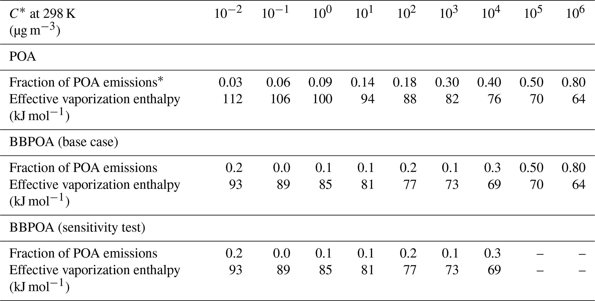
∗ This is the traditional nonvolatile POA included in inventories used for regulatory purposes. The sum of all fractions can exceed unity because a large fraction of the IVOCs is not included in these traditional particle emission inventories.
The partitioning calculations of primary emissions are performed using the same module used to calculate the partitioning of all semi-volatile organic species (Koo et al., 2003). This is based on absorptive partitioning theory and assumes that the bulk gas and particle phases are in equilibrium and all condensable organics form a pseudo-ideal solution (Odum et al., 1996; Strader et al., 1999). Organic gas–particle partitioning is assumed to depend on temperature and aerosol composition. The partioning model assumes that the organic compounds form a single pseudo-ideal solution in the particle phase and do not interact with the aqueous phase (Strader et al., 1999). The Clausius–Clapeyron equation is used to describe the effects of temperature on C∗ and partitioning. Table 1 also lists the enthalpies of vaporization currently used in PMCAMx and PMCAMx-SR. All POA species are assumed to have an average molecular weight of 250 g mol−1.
2.1.2 Secondary organic aerosol from VOCs
Based on the original work of Lane et al. (2008a), SOA from VOCs (SOA-v) is represented using four volatility bins (1, 10, 102, 103 µg m−3 at 298 K). The model uses four surrogate compounds for SOA from anthropogenic VOCs (ASOA-v) and another four for SOA from biogenic VOCs (BSOA-v). These can exist in either the gas or particulate phase so there are two model variables for each volatility bin. Additional surrogate compounds, and thus model variables, are used to keep track of the oxidation products of anthropogenic IVOCs (SOA-iv) and SVOCs (SOA-sv). PMCAMx-SR includes additional SOA surrogate compounds to simulate the oxidation products of the biomass burning emissions. ASOA components are assumed to have an average molecular weight of 150 g mol−1, while BSOA species have 180 g mol−1. Laboratory results from the smog-chamber experiments of Ng et al. (2006) and Hildebrandt et al. (2009) are used for the anthropogenic aerosol yields.
2.1.3 Chemical aging mechanism
All OA components are treated as chemically reactive in PMCAMx-SR. Anthropogenic SOA components resulting from the oxidation of SVOCs and IVOCs (ASOA-sv, ASOA-iv) are assumed to react with OH radicals in the gas phase with a rate constant of cm3 mol−1 s−1, resulting in the formation of lower-volatility ASOA. Semi-volatile anthropogenic ASOA-v components are assumed to react with OH in the gas phase with a rate constant of cm3 mol−1 s−1 (Atkinson and Arey, 2003). All these aging reactions are assumed to reduce the volatility of the reacted vapor by 1 order of magnitude, which is linked to an increase in OA mass by approximately 7.5 % to account for added oxygen. BSOA-v aging is assumed to lead to zero net change of volatility and OA mass (Lane et al., 2008b).
2.2 PMCAMx-SR enhancements
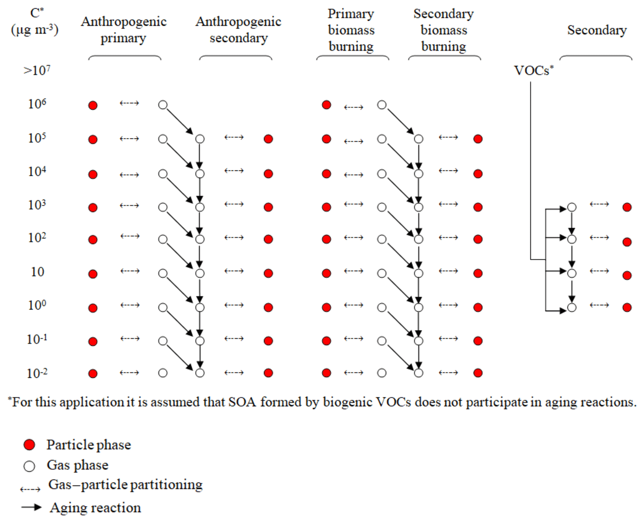
In PMCAMx-SR, the fresh biomass burning organic aerosol (BBOA) and its secondary oxidation products (BBSOA) are simulated separately from the other POA components. The May et al. (2013) volatility distribution is used to simulate the gas–particle partitioning of fresh BBOA. This distribution includes surrogate compounds up to a volatility of 104 µg m−3. This means that the more volatile IVOCs, which could contribute to SOA formation, are not included. To close this gap, the values of the volatility distribution of Robinson et al. (2007) are used for the 105 and 106 µg m−3 bins (Table 1). The sensitivity of PMCAMx-SR to the IVOC emissions added to the May et al. (2013) distribution will be explored in a subsequent section. The effective saturation concentrations and the enthalpies of vaporization used for BBOA in PMCAMx-SR are also listed in Table 1. The new BBOA scheme requires the introduction of 36 new organic species to simulate both phases of fresh primary and oxidized BBOA components. The rate constant used for the chemical aging reactions is the same as the one currently used for all POA components and has a value of cm3 mol−1 s−1. The volatility distributions of BBOA in PMCAMx and PMCAMx-SR are shown in Fig. 1a. The volatility distribution implemented in PMCAMx-SR results in less volatile BBOA for ambient OA levels (a few µg m−3) (Fig. 1b). A schematic representation of the organic aerosol module of PMCAMx-SR is shown in Fig. 2.
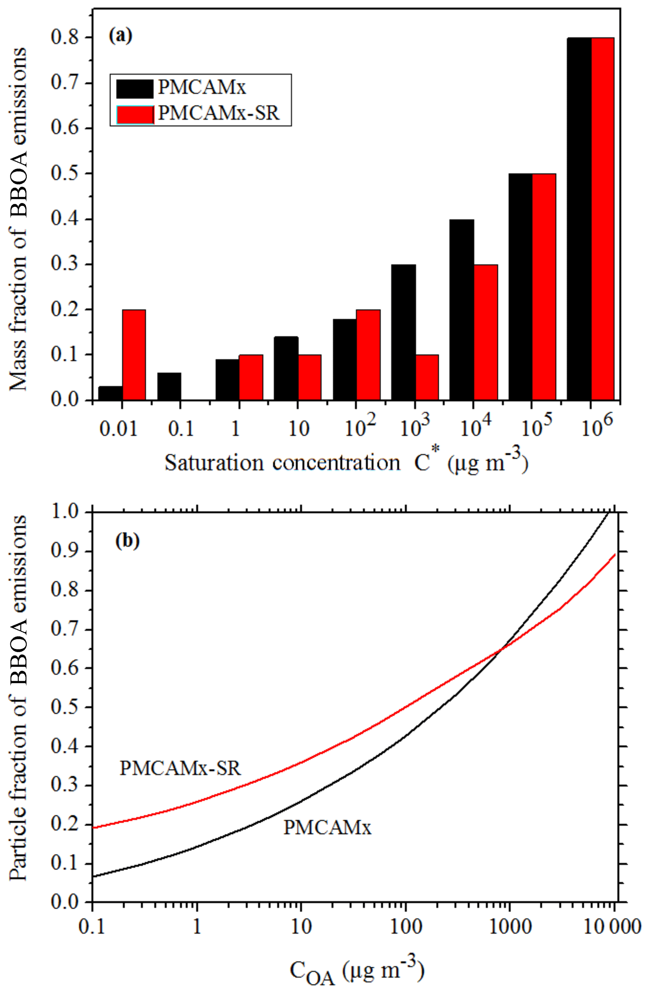
Figure 1(a) Volatility distribution of BBOA in PMCAMx and PMCAMx-SR. (b) Particle fractions of BBOA emissions as a function of OA concentration at 298 K.
PMCAMx-SR was applied to a 5400 km×5832 km2 region covering Europe with 36 km×36 km grid resolution and 14 vertical layers extending up to 6 km. The model was set to perform simulations on a rotated polar stereographic map projection. The necessary inputs to the model include horizontal wind components, temperature, pressure, water vapor, vertical diffusivity, clouds, and rainfall. All meteorological inputs were created using the meteorological model WRF (Weather Research and Forecasting) (Skamarock et al., 2005). The simulations were performed during a summer period (1–29 May 2008) and a winter period (25 February–22 March 2009). In order to limit the effect of the initial conditions on the results, the first 2 d of each simulation were excluded from the analysis.
Anthropogenic and biogenic emissions in the form of hourly gridded fields were developed both for gases and primary particulate matter. Anthropogenic gas emissions include land emissions from the GEMS dataset (Visschedijk et al., 2007) and also emissions from international shipping activities. Anthropogenic particulate matter mass emissions of organic and elemental carbon are based on the Pan-European Carbonaceous Aerosol Inventory (Denier van der Gon et al., 2010) that has been developed as part of the EUCAARI project activities (Kulmala et al., 2009). All relevant significant emission sources, including anthropogenic biomass burning emissions from agricultural activities and residential heating, are included in the two inventories. Day-specific wildfire emissions were also included (Sofiev et al., 2008a, b). Emissions from ecosystems were calculated offline by MEGAN (Model of Emissions of Gases and Aerosols from Nature) (Guenther et al., 2006). The marine aerosol emission model developed by O'Dowd et al. (2008) has been used to estimate mass fluxes for both accumulation and coarse mode including the organic aerosol fraction. Wind speed data from WRF and chlorophyll a concentrations are the inputs needed for the marine aerosol emissions module.
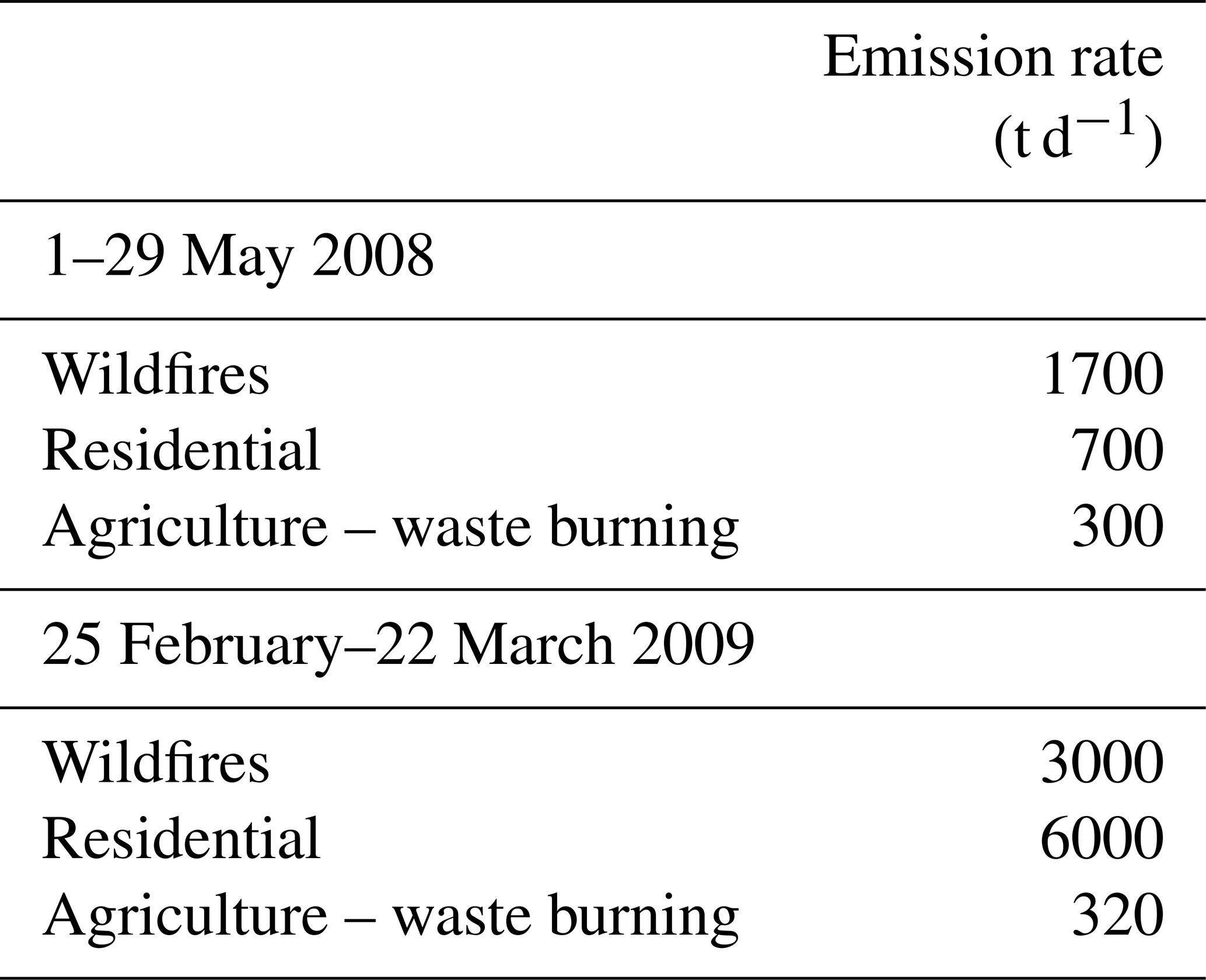
The gridded emission inventories of BBOA species for the two modeled periods are shown in Fig. 3. During the early summer simulated period wildfires were responsible for 60 % of the BBOA emissions, agricultural waste burning for 15 %, and residential wood combustion for 25 % (Table 2). Details about the OA emission rates from agricultural activities are provided in the Supplement (Fig. S1). During winter, residential combustion is the dominant source (63 %). The wintertime wildfire emissions in the inventory, approximately 3000 t d−1, are quite high especially when compared with the corresponding summer value which is 1700 t d−1. The spatial distribution of OA emission rates from wildfires during 25 February–22 March 2009 is provided in the Supplement (Fig. S2). Analysis of fire counts in satellite observations used for the development of the inventory suggests that some agricultural emissions have probably been attributed to wildfires. All BBOA sources are treated the same way in PMCAMx-SR, so this potential misattribution does not affect our results.
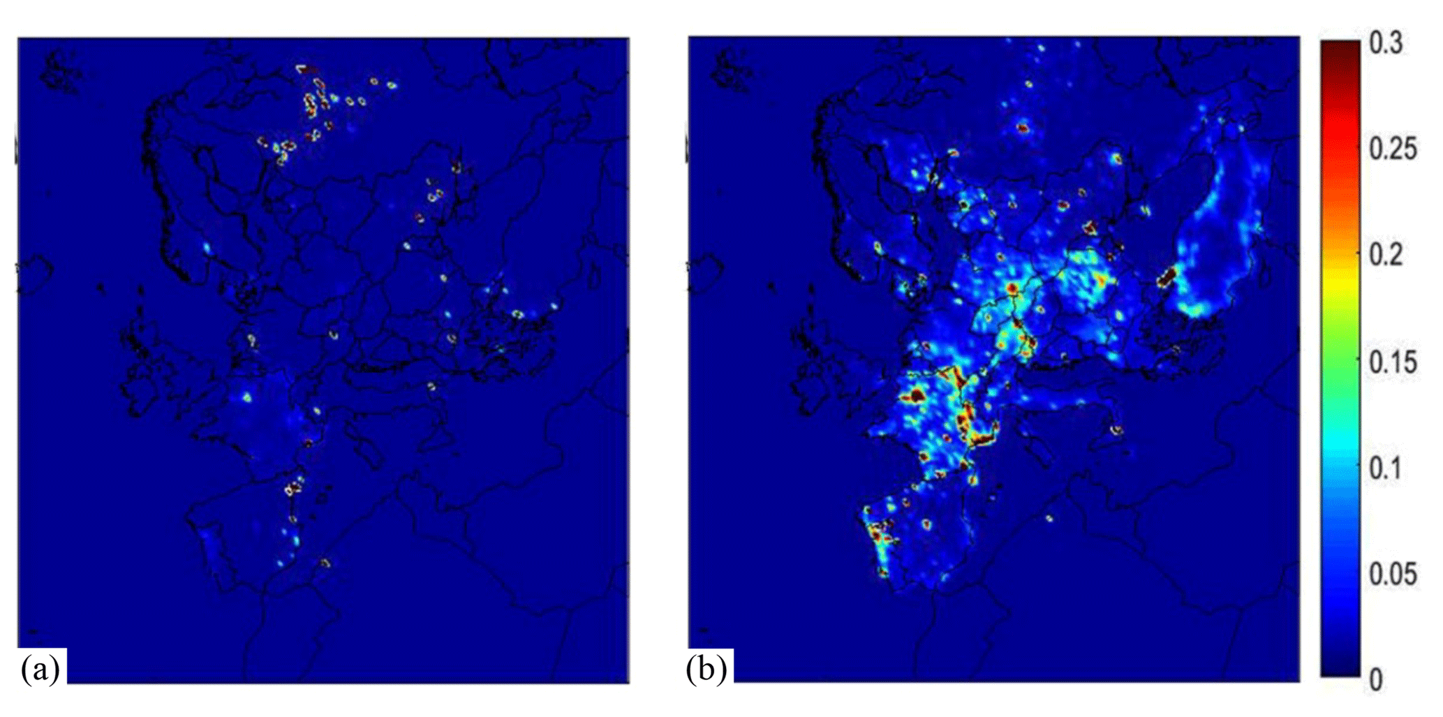
Figure 3Spatial distribution of average biomass burning OA emission rates (kg d−1 km−2) for the two simulation periods: (a) 1–29 May 2008 and (b) 25 February–22 March 2009.
Table 2Organic compound emission rates (in t d−1) over the modeling domain during the simulated periods.
To test our implementation of the source-resolved VBS in PMCAMx-SR we compared its results with those of PMCAMx using the same VBS parameters. For this test using PMCAMx-SR, we used the default PMCAMx BBOA partitioning parameters shown in Table 1, as proposed by Shrivastava et al. (2008). In this way both models should simulate the BBOA in exactly the same way, but PMCAMx-SR describes it independently while PMCAMx lumps it with other primary OA. The differences between the corresponding OA concentrations predicted by the two models were on average less than 10−3 µg m−3 (0.03 %). The maximum difference was approximately 0.03 µg m−3 (0.6 %) in western Germany. This suggests that our changes to the code of PMCAMx to develop PMCAMx-SR did not introduce any inconsistencies with the original model. The small differences are due to numerical issues in the advection/dispersion calculations.
In this section the predictions of PMCAMx-SR for the base case simulations during 1–29 May 2008 and 25 February–22 March 2009 are analyzed. Figure 4 shows the PMCAMx-SR predicted average ground-level PM2.5 concentrations for the various OA components for the two simulated periods.
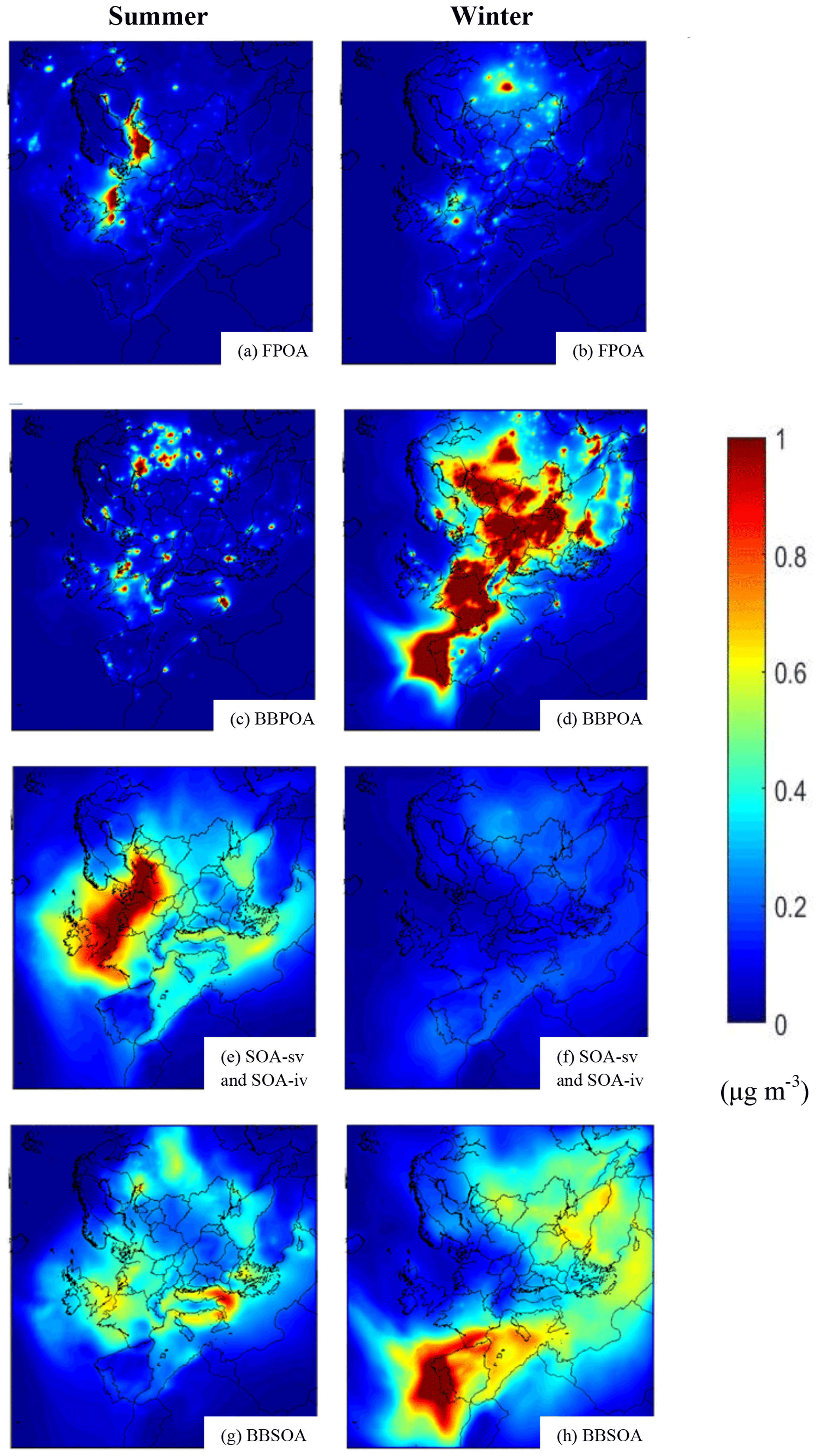
Figure 4PMCAMx-SR predicted base case ground-level concentrations of PM2.5 (a–b) FPOA, (c–d) BBPOA, (e–f) SOA, and (g–h) BBSOA during the modeled summer and winter periods.
The POA from non-BBOA sources will be called fossil POA (FPOA) in the rest of the paper. FPOA levels over Europe were on average around 0.1 µg m−3 during both periods (Fig. 4a and b). However, their spatial distributions are quite different. During May, predicted FPOA concentrations are as high as 2 µg m−3 in polluted areas in central and northern Europe but are less than 0.5 µg m−3 in the rest of the domain. These low levels are due to the evaporation of POA in this warm period. For the winter period peak FPOA levels are higher, reaching values of around 3.5 µg m−3 in Paris and Moscow. FPOA contributes approximately 3.5 % and 6 % to total OA in Europe during May 2008 and February–March 2009, respectively. BBPOA concentrations have peak average values 7 µg m−3 in St. Petersburg, Russia, and 10 µg m−3 in Porto, Portugal, during summer and winter, respectively (Fig. 4c and d). During the summer BBPOA is predicted to contribute 5 % to total OA and its contribution during winter increases to 32 %. The average predicted BBOA concentrations over Europe are 0.1 and 0.8 µg m−3 during the summer and the winter period, respectively.
The SOA resulting from the oxidation of IVOCs (SOA-iv) and evaporated POA (SOA-sv) has concentrations as high as 1 µg m−3 in Central Europe and the average levels are around 0.3 µg m−3 (13 % contribution to total OA) during summer (Fig. 4e). During winter the peak concentration value was a little less than 0.5 µg m−3 in Moscow, Russia, and the average levels were approximately 0.1 µg m−3 (5.5 % contribution to total OA) (Fig. 4f). The highest average concentration of BBSOA-sv and BBSOA-iv (biomass burning SOA from intermediate volatility and semi-volatile precursors) was approximately 1 µg m−3 in Lecce, Italy, during summer and 3.5 µg m−3 in Porto during winter. During May BBSOA is predicted to contribute 11 % to total OA over Europe and during February–March 2009 its predicted contribution is 15 %. The average BBSOA is 0.3 µg m−3 during summer and approximately 0.4 µg m−3 during winter (Fig. 4g and h). During the summer, the remaining 67 % of total OA is biogenic SOA (52 %) and anthropogenic SOA (15 %) and in winter, of the remaining 41 % of total OA, 36 % is biogenic and 5 % is anthropogenic SOA (not shown).
In areas like St. Petersburg, Russia, predicted hourly BBOA levels exceeded 300 µg m−3 due to the nearby fires affecting the site on 3–5 May (Fig. 5a). For these extremely high concentrations, most of the BBOA (90 % for St. Petersburg) was primary, with the BBSOA contributing around 10 %. The spatiotemporal evolution of BBPOA and BBSOA during 1–6 May in Scandinavia and northwestern Russia is depicted in Fig. 6. A series of fires started in Russia on 1 May, becoming more intense during the next days until 6 May when they were mostly extinguished. BBSOA, as expected, follows the opposite evolution, with low concentration values in the beginning of the fire events (1 May) and higher values later on. The BBSOA production increases the range of influence of the fires.
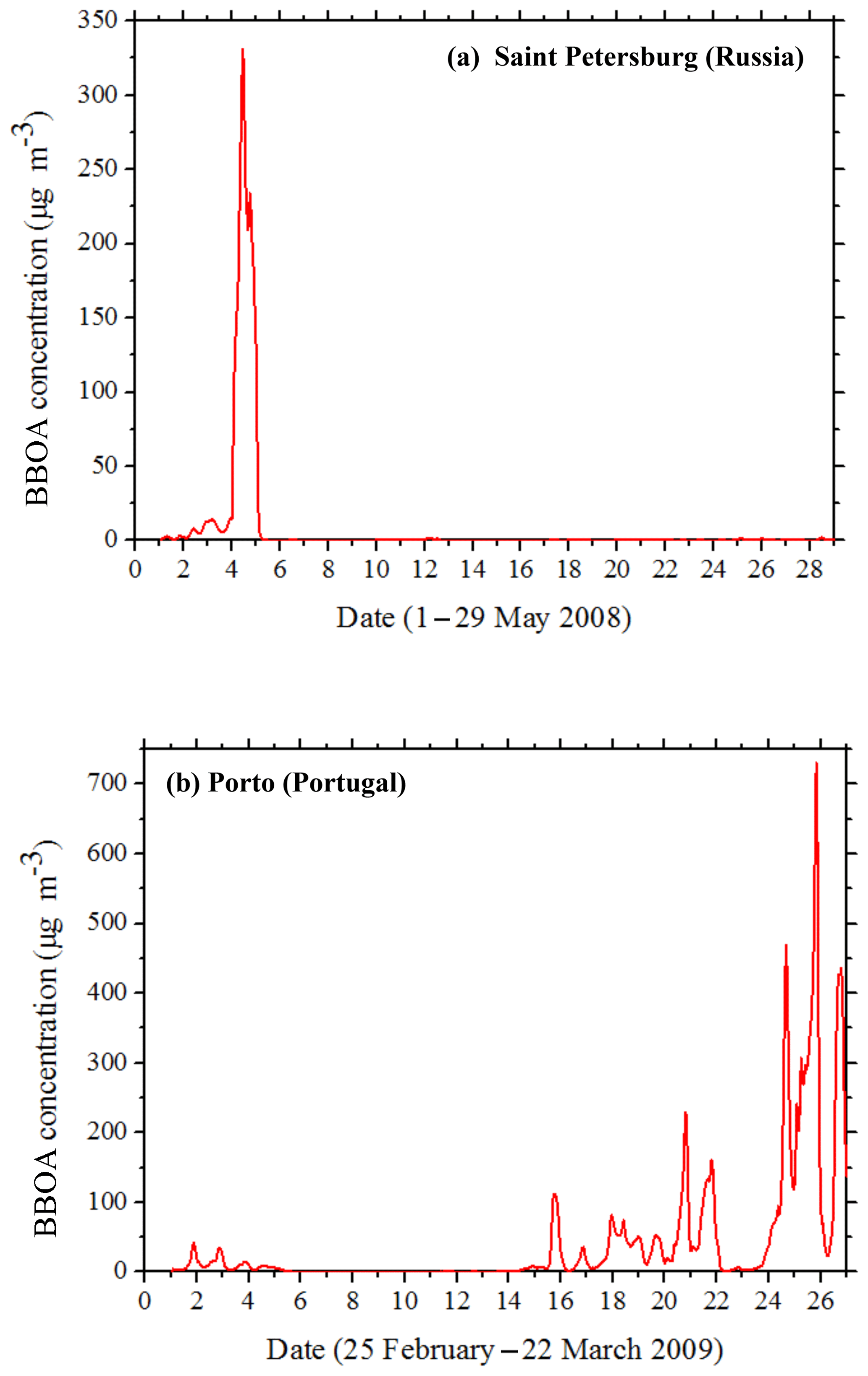
Figure 5Time series of PM2.5 BBOA concentrations in (a) Saint Petersburg, Russia, during 1–29 May 2008 and in (b) Porto, Portugal, during 25 February–22 March 2009.
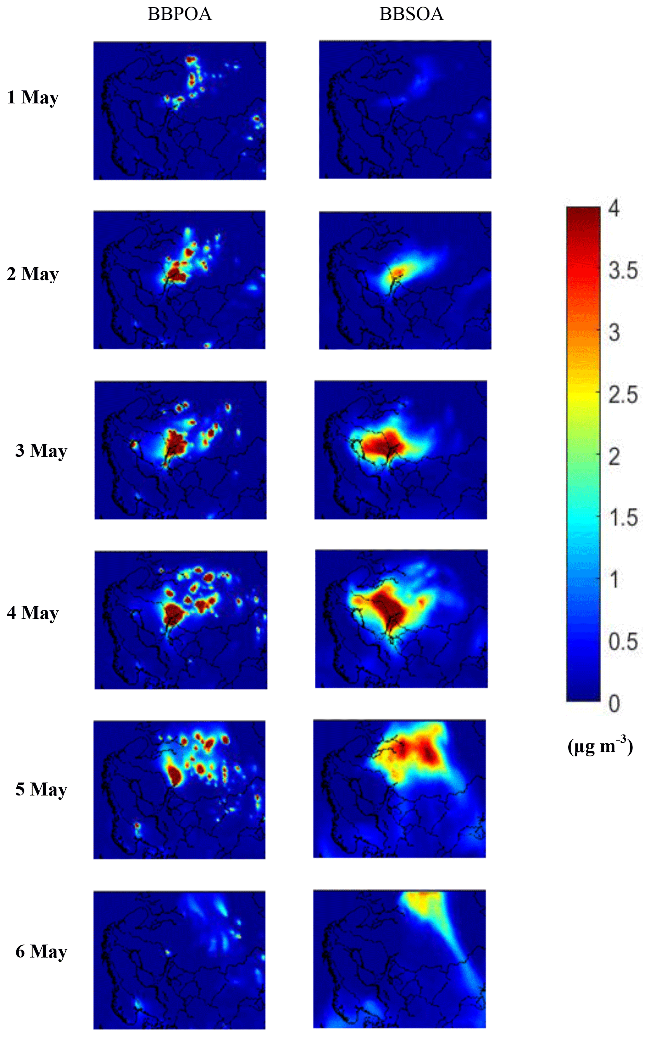
Figure 6PMCAMx-SR predicted base case ground-level concentrations of PM2.5 BBPOA and BBSOA during 1–6 May 2008 from the Scandinavian Peninsula and Russia.
In Majden (North Macedonia) fires contributed up to 25 µg m−3 of BBOA on 25–26 May. The BBSOA was 15 % of the BBOA in this case (Fig. S3). Fires also occurred in southern Italy (Catania) and contributed up to 52 µg m−3 of OA on 15–17 May. During this period the BBSOA was 13 % of the BBOA (Fig. S3). Paris (France) and Dusseldorf (Germany) were further away from major fires but were also affected by fire emissions during most of the month (Fig. S3). The maximum hourly BBOA levels in these cities were around 5 µg m−3, but BBSOA in this case represents, according to the model, around 35 % of the total BBOA in Paris and 55 % in Dusseldorf.
During the winter simulation period, there were major fires during 20–22 March in Portugal and northwestern Spain. The maximum predicted hourly BBOA concentration in Porto (Portugal) exceeded 700 µg m−3 on March 21 (Fig. 5b). During the same 3 d in March, the average levels of BBPOA in Portugal and Spain were 9 µg m−3 and their contribution to total OA was 62 %. BBPOA was 80 % of the total BBOA during 20–22 March in the Iberian Peninsula.
We performed an additional sensitivity simulation, where we assumed that there are no emissions of more volatile IVOCs (those in the 105 and 106 µg m−3 bins). The partitioning parameters used in this sensitivity test are shown in Table 1. The emissions rates for each volatility bin during the two modeled periods are provided in the Supplement (Table S1). The absolute emissions assigned to the lower-volatility bins are approximately the same for both simulations. More specifically, during May 2008, the emission rates of LVOCs (10−2, 10−1 µg m−3 C∗ bins) and SVOCs (100, 101, 102 µg m−3 C∗ bins) are 530 and 1050 t d−1, respectively, for the base case run and 580 and 1160 t d−1, respectively, for the sensitivity run. During February–March 2009, the emission rates of LVOCs and SVOCs are 2100 and 4100 t d−1, respectively, for the base case run and 2300 and 4500 t d−1, respectively, for the sensitivity run. The base case simulation assumes higher emissions in the upper volatility bins of the IVOCs (103, 104, 105, 106 µg m−3 C∗ bins) which can be converted to BBSOA. During summer, the emission rate of IVOCs is 4460 t d−1 in the base case run and 1160 t d−1 in the sensitivity test. During winter, the emission rate of IVOCs is 17 400 t d−1 in the base case and 4500 t d−1 in the sensitivity test.
The base case and the sensitivity simulations predict practically the same BBPOA concentrations in both periods (Fig. 7), as expected based on the emission inventory. During summer, the average absolute change of BBPOA in Europe is around 10 % (corresponding to 0.01 µg m−3) (Fig. 7a). The average difference in BBSOA is significantly higher and around 60 % (0.2 µg m−3 on average) due to the higher IVOC emissions of the base case simulation. The atmospheric conditions during this warm summer period (high temperature, UV radiation, relative humidity) lead to high OH concentrations and rapid production of BBSOA.
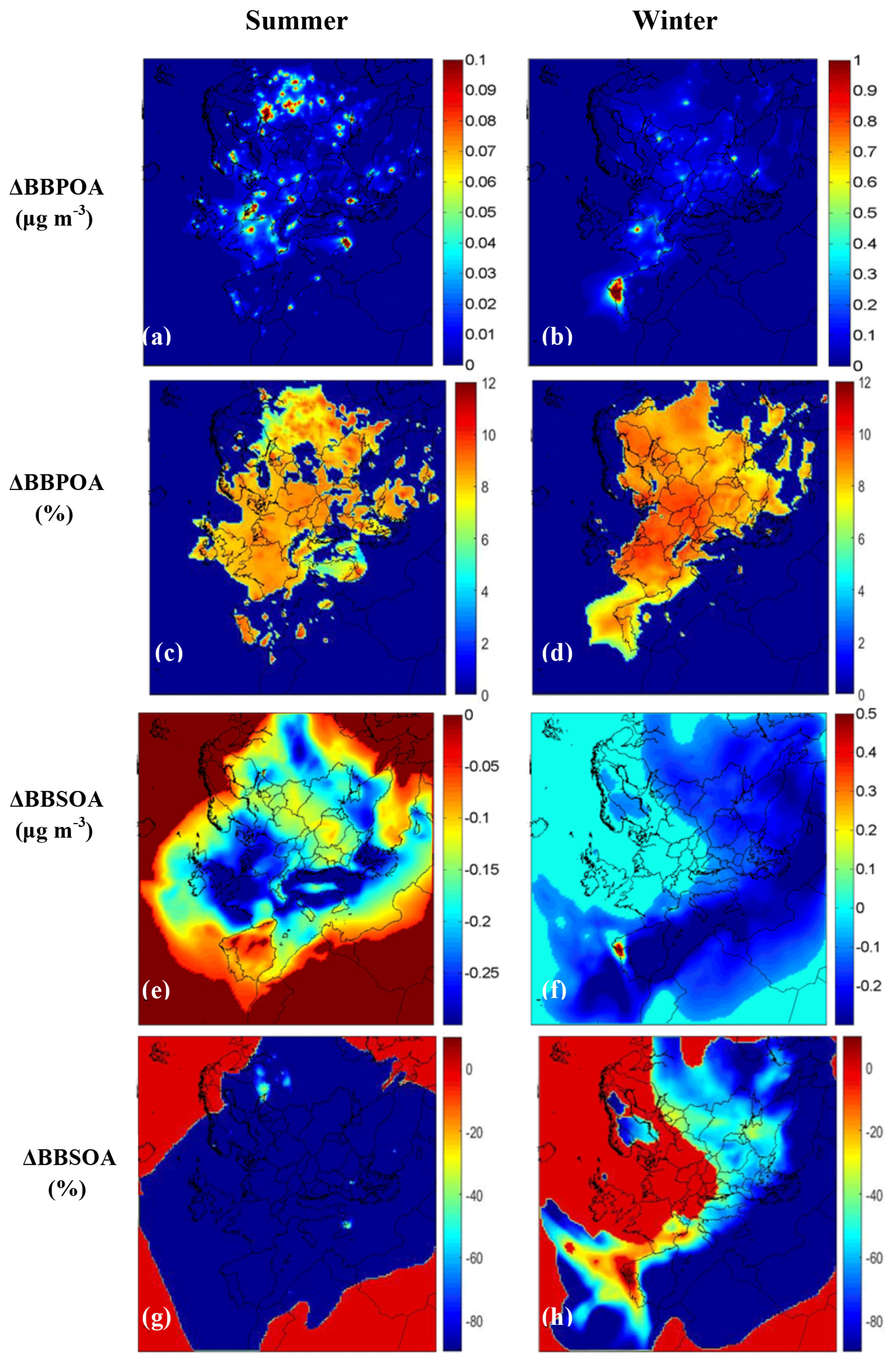
Figure 7Average predicted absolute (µg m−3) difference (sensitivity case minus base case) of ground-level PM2.5 (a–b) BBPOA and (e–f) BBSOA concentrations from PMCAMx-SR base case and sensitivity simulations during the modeled periods. Also shown are the corresponding relative (%) change of ground-level PM2.5 (c–d) BBPOA and (g–h) BBSOA concentrations during the modeled periods. Positive values indicate that the PMCAMx-SR sensitivity run predicts higher concentrations.
During winter, the average absolute change for both BBPOA and BBSOA in Europe is approximately 0.1 µg m−3 (Fig. 7b and f). These correspond to 15 % change for the primary and 25 % for the secondary BBOA levels. The maximum difference for average BBPOA is approximately 5 µg m−3 and for BBSOA it is around 1.5 µg m−3 (both in northwestern Portugal). However, during the fire period (20–22 March) in Spain and Portugal, the maximum concentration difference between the two cases was 20 µg m−3 for BBPOA and 7 µg m−3 for BBSOA.
Figure 8 shows the total BBOA (sum of BBPOA and BBSOA) during both periods. Higher BBOA concentrations are predicted in the base case simulation due to the higher BBSOA concentrations from higher IVOC emissions. During summer the contributions of the biomass burning IVOC oxidation products to total BBOA exceed 30 % over most of Europe, while during winter these components are important mostly over southern Europe and the Mediterranean (Fig. S4).
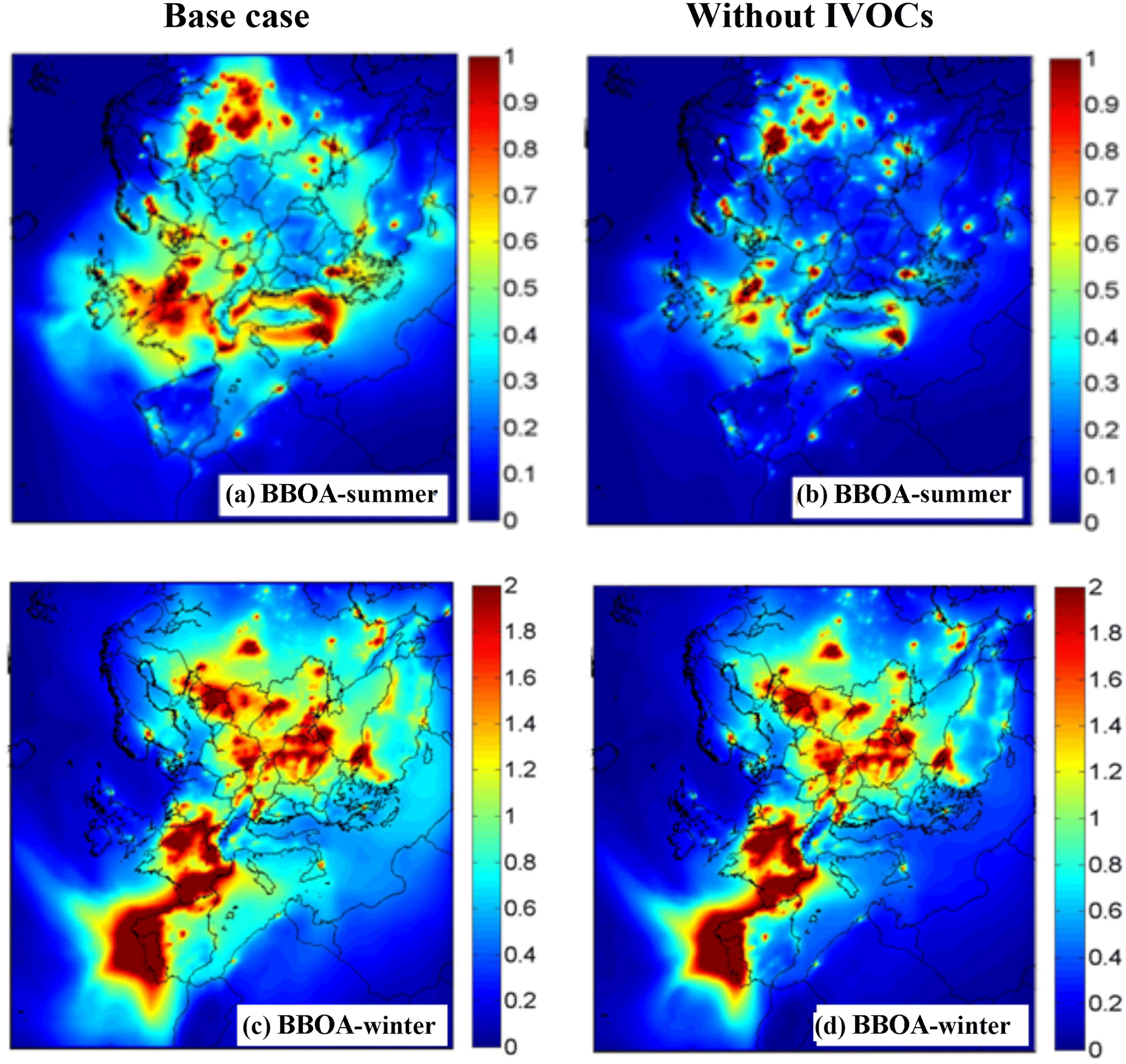
Figure 8Predicted ground-level concentrations of PM2.5 total BBOA (µg m−3) during the modeled summer period (a–b) and the modeled winter (c–d) period. The figures to the left are for the PMCAMx-SR base case simulation while those to the right are for the low-IVOC sensitivity test.
In order to assess the PMCAMx-SR performance during the two simulation periods, the model's predictions were compared with AMS hourly measurements that took place at several sites around Europe. All observation sites are representative of regional atmospheric conditions.
The Positive Matrix Factorization (PMF) technique (Paatero and Tapper, 1994; Lanz et al., 2007; Ulbrich et al., 2009; Ng et al., 2010) was used to analyze the AMS organic spectra providing information about the sources contributing to the OA levels (Hildebrandt et al., 2010; Morgan et al., 2010). The method classifies OA into different types based on different temporal emission and formation patterns and separates it into hydrocarbon-like organic aerosol (HOA – a POA surrogate), oxidized organic aerosol (OOA – a SOA surrogate) and fresh BBOA. Additionally, factor analysis can further classify OOA into more and less oxygenated OOA components. Fresh BBOA can be compared directly to the PMCAMx-SR BBPOA predictions, whereas BBSOA should, in principle at least, be included in the OOA factors. The AMS HOA can be compared with predicted fresh POA. The oxygenated AMS OA component can be compared against the sum of anthropogenic and biogenic SOA (ASOA, BSOA), SOA-sv and SOA-iv, BBSOA, and OA from long range transport.
PMCAMx-SR performance is quantified by calculating the mean bias (MB), the mean absolute gross error (MAGE), the fractional bias (FBIAS), and the fractional error (FERROR) defined as follows:
where Pi is the predicted value of the pollutant concentration, Oi is the observed value, and n is the number of measurements used for the comparison. AMS measurements are available from four stations (Cabauw, Finokalia, Melpitz, and Mace Head) during 1–29 May 2008 and seven stations (Cabauw, Helsinki, Mace Head, Melpitz, Hyytiälä, Barcelona and Chilbolton) during 25 February–23 March 2009 (Crippa et al., 2014).
During May 2008 a BBPOA factor was identified based on the PMF analysis of the measurements only in Cabauw and Mace Head. In the other two sites (Finokalia and Melpitz) PMCAMx-SR predicted very low average BBPOA levels (less than 0.1 µg m−3), so its predictions for these sites can be viewed as consistent with the results of the PMF analysis. Figure 9 shows the comparison of the predicted BBPOA by PMCAMx-SR with the observed values in Cabauw. The average AMS-PMF BBOA was 0.4 µg m−3 and the predicted average BBPOA by PMCAMx-SR was also 0.4 µg m−3. The mean bias was only −0.01 µg m−3. The model, however, tended to overpredict during the first 10 d and to underpredict during the last week. In Mace Head PMCAMx-SR predicts high BBOA levels during 14–15 May, but, unfortunately, the available measurements started on 16 May. During the last 2 weeks of the simulation the model predicts much lower BBOA levels (approximately 0.35 µg m−3 less) than the AMS-PMF analysis. The same problem was observed in Cabauw, suggesting potential problems with the fire emissions during this period.
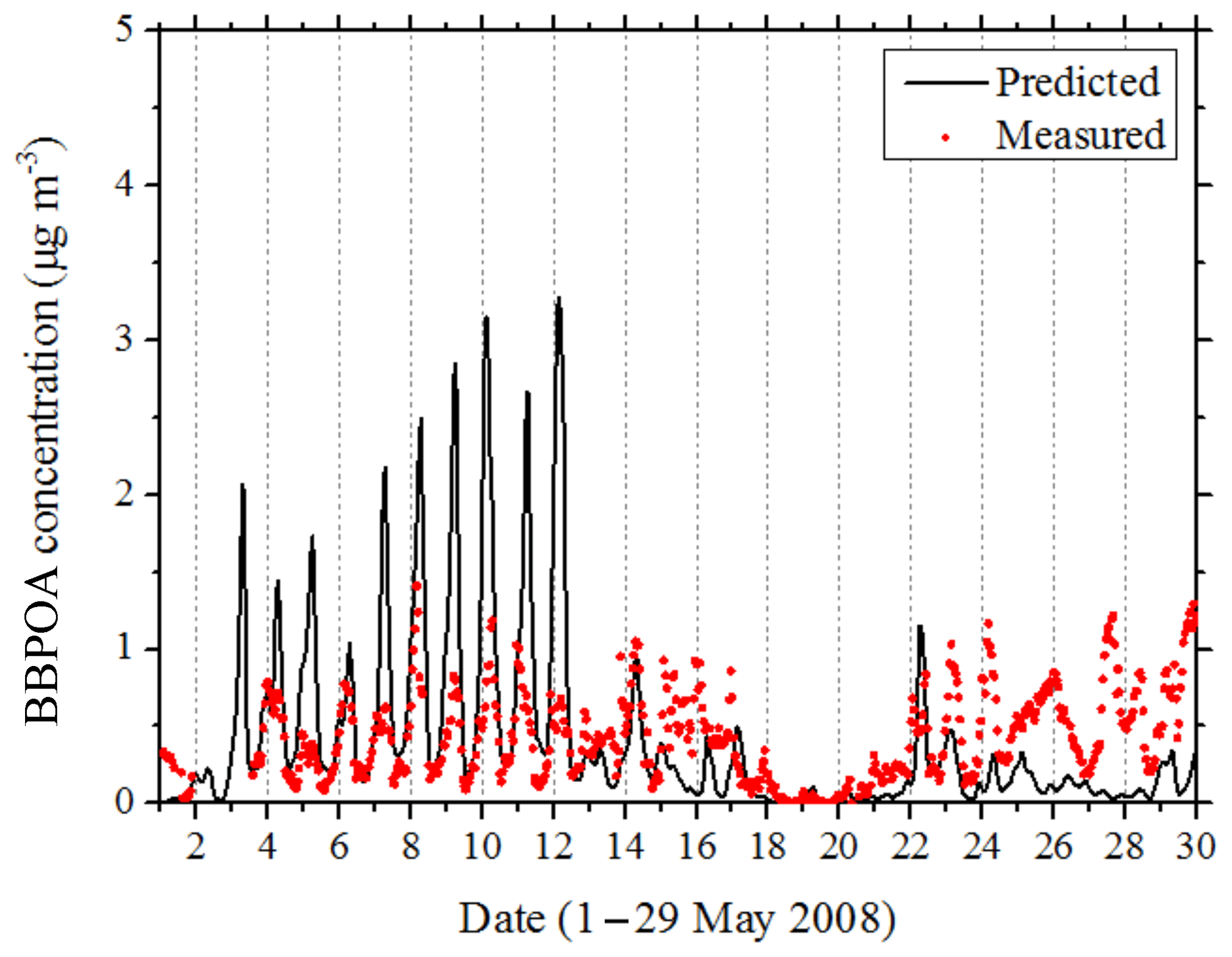
Figure 9Comparison of hourly BBPOA concentrations predicted by PMCAMx-SR with values estimated by PMF analysis of the AMS data in Cabauw during 1–29 May 2008.
During winter the model tends to overpredict the observed BBOA values in Barcelona, Cabauw, Melpitz, Helsinki and Hyytiälä. On the other hand, the model underpredicts the BBOA in Mace Head and Chibolton by approximately 0.3 µg m−3 on average. The prediction skill metrics of PMCAMx-SR (base case and sensitivity test) against AMS factor analysis during the modeled periods are also provided in the Supplement (Tables S2–S5). These problems in reproducing wintertime OA measurements were also noticed by Denier van der Gon et al. (2015) and suggest problems in the emissions and/or the simulation of the BBOA during this cold period with slow photochemistry.
Given that BBOA contributed, on average, less than half of the total OA during the summer, the performance (fractional bias and error) for OA of PMCAMx-SR (both for the base case and the sensitivity test) was quite similar to that of the original PMCAMx (Table S6). The performance of the sensitivity test was a little better, suggesting that the BBSOA production from the corresponding IVOCs could be overpredicted. However, this can be also due to other sources of error in the model. The situation was similar during the winter. There was a small reduction in the already small fractional bias but overall the performance of PMCAMx-SR for OA and OOA were quite similar to that of PMCAMx (Table S7). This, however, suggests that the errors in the OA predictions are not due to the new treatment of BBOA but rather to other errors that are also present in the original model.
A source-resolved version of PMCAMx, called PMCAMx-SR was developed and tested. This new version can be used to study specific OA sources independently (e.g., diesel emissions) if so desired by the user. We applied PMCAMx-SR to the European domain during an early summer and a winter period focusing on biomass burning.
The concentrations of BBOA (sum of BBPOA and BBSOA) and their contributions to total OA over Europe are, as expected, quite variable in space and time. During the early summer, the contribution of BBOA to total OA over Europe was predicted to be 16 %, while during winter it increased to 47 %. Secondary biomass burning OA was predicted to be approximately 70 % of the BBOA during summer and only 30 % during the winter on average. The production of BBSOA increases the range of influence of fires.
The IVOCs emitted by the fires can be a major source of SOA. In our simulations, the IVOCs with saturation concentrations and 106 µg m−3 contributed approximately one third of the average BBOA over Europe. The emissions of these compounds and their aerosol forming potential are uncertain, so the formation of BBSOA clearly is an important topic for future work.
PMCAMx-SR was evaluated against AMS measurements taken at various European measurement stations and the results of the corresponding PMF analysis. During the summer the model reproduced without bias the average measured BBPOA levels in Cabauw and the practically zero levels in Finokalia and Melpitz. However, it underpredicted the BBPOA in Mace Head. Its performance for oxygenated organic aerosol (OOA) which should include BBSOA together with a lot of other sources was mixed: overprediction in Cabauw (fractional bias +42 %), Mace Head (fractional bias +34 %), and Finokalia (fractional bias +23 %) and underprediction in Melpitz (fractional bias −14 %).
During the winter the model overpredicted the BBPOA levels in most stations (Cabauw, Helsinki, Melpitz, Hyytiälä, Barcelona), while it underpredicted in Mace Head and Chibolton. At the same time, it reproduced the measured OOA concentrations with less than 15 % bias in Cabauw, Helsinki, and Hyytiälä, underpredicted OOA in Melpitz, Barcelona, and Chibolton and overpredicted OOA in Mace Head. These results both potential problems with the wintertime emissions of BBPOA and the production of secondary OA during the winter.
The data in the study are available from the authors upon request (spyros@chemeng.upatras.gr).
The supplement related to this article is available online at: https://doi.org/10.5194/acp-19-5403-2019-supplement.
GNT conducted the simulations, analyzed the results, and wrote the paper. SNP was responsible for the design of the study, the synthesis of the results, and contributed to the writing of the paper.
The authors declare that they have no conflict of interest.
This article is part of the special issue “Simulation chambers as tools in atmospheric research (AMT/ACP/GMD inter-journal SI)”. It is not associated with a conference.
This study was financially supported by the European Union's Horizon 2020 EUROCHAMP–2020 Infrastructure Activity (grant agreement 730997) and the Western Regional Air Partnership (WRAP Project no. 178-14).
This paper was edited by Jacqui Hamilton and reviewed by two anonymous referees.
Alvarado, M. J., Lonsdale, C. R., Yokelson, R. J., Akagi, S. K., Coe, H., Craven, J. S., Fischer, E. V., McMeeking, G. R., Seinfeld, J. H., Soni, T., Taylor, J. W., Weise, D. R., and Wold, C. E.: Investigating the links between ozone and organic aerosol chemistry in a biomass burning plume from a prescribed fire in California chaparral, Atmos. Chem. Phys., 15, 6667–6688, https://doi.org/10.5194/acp-15-6667-2015, 2015.
Andreae, M. O. and Crutzen, P. J.: Atmospheric aerosols: biogeochemical sources and role in atmospheric chemistry, Science, 276, 1052–1058, 1997.
Atkinson, R. and Arey, J.: Atmospheric degradation of volatile organic compounds, Chem. Rev., 103, 4605–4638, 2003.
Bond, T. C., Streets, D. G., Yarber, K. F., Nelson, S. M., Woo, J. H., and Klimont, Z.: A technology-based global inventory of black and organic carbon emissions from combustion, J. Geophys. Res., 109, D14203, https://doi.org/10.1029/2003JD003697, 2004.
Carter, W. P. L.: Programs and files implementing the SAPRC-99 mechanism and its associated emissions processing procedures for Models-3 and other regional models, available at: http://www.cert.ucr.edu/~carter/SAPRC99/ (last access: 20 April 2019), 2000.
Crippa, M., Canonaco, F., Lanz, V. A., Äijälä, M., Allan, J. D., Carbone, S., Capes, G., Ceburnis, D., Dall'Osto, M., Day, D. A., DeCarlo, P. F., Ehn, M., Eriksson, A., Freney, E., Hildebrandt Ruiz, L., Hillamo, R., Jimenez, J. L., Junninen, H., Kiendler-Scharr, A., Kortelainen, A.-M., Kulmala, M., Laaksonen, A., Mensah, A. A., Mohr, C., Nemitz, E., O'Dowd, C., Ovadnevaite, J., Pandis, S. N., Petäjä, T., Poulain, L., Saarikoski, S., Sellegri, K., Swietlicki, E., Tiitta, P., Worsnop, D. R., Baltensperger, U., and Prévôt, A. S. H.: Organic aerosol components derived from 25 AMS data sets across Europe using a consistent ME-2 based source apportionment approach, Atmos. Chem. Phys., 14, 6159–6176, https://doi.org/10.5194/acp-14-6159-2014, 2014.
Denier van der Gon, H. A. C, Visschedijk, A., van der Brugh, H., and Droge, R.: A high resolution European emission data base for the year 2005, TNO report TNO-034-UT-2010-01895 RPTML, Utrecht, the Netherlands, 2010.
Denier van der Gon, H. A. C., Bergström, R., Fountoukis, C., Johansson, C., Pandis, S. N., Simpson, D., and Visschedijk, A. J. H.: Particulate emissions from residential wood combustion in Europe – revised estimates and an evaluation, Atmos. Chem. Phys., 15, 6503–6519, https://doi.org/10.5194/acp-15-6503-2015, 2015.
Dockery, W. D., Pope, C. A., Xu, X., Spengler, J. D., Ware, J. H., Fay Jr., M. E., Ferris, B. G., and Speizer, F. E.: An association between air pollution and mortality in six U.S. cities, New Engl. J. Med., 329, 1753–1759, 1993.
Dockery, D. W., Cunningham J., Damokosh A. I., Neas L. M., Spengler J. D., Koutrakis P., Ware J. H., Raizenne M., and Speizer F. E.: Health effects of acid aerosols on North America children: Respiratory symptoms, Environ. Health Persp., 104, 26821–26832, 1996.
Donahue, N. M., Robinson, A. L., Stanier, C. O., and Pandis, S. N.: Coupled partitioning, dilution, and chemical aging of semivolatile organics, Environ. Sci. Technol., 40, 2635–2643, 2006.
ENVIRON: User's Guide to the Comprehensive Air Quality Model with Extensions (CAMx), Version 4.02, Report, ENVIRON Int. Corp., Novato, Calif., available at: http://www.camx.com (last access: 20 April 2019), 2003.
Fahey, K. and Pandis, S. N.: Optimizing model performance: variable size resolution in cloud chemistry modelling, Atmos. Environ., 35, 4471–4478, 2001.
Fountoukis, C., Butler, T., Lawrence, M. G., Denier van der Gon, H. A. C., Visschedijk, A. J. H., Charalampidis, P., Pilinis, C., and Pandis, S. N.: Impacts of controlling biomass burning emissions on wintertime carbonaceous aerosol in Europe, Atmos. Environ., 87, 175–182, 2014.
Gauderman, W. J., McConnel R., Gilliland F., London S., Thomas D., Avol E., Vora H., Berhane K., Rappaport E. B., Lurmann F., Margolis H. G., and Peters J.: Association between air pollution and lung function growth in southern California children, Am. J. Resp. Crit. Care, 162, 1383–1390, 2000.
Gaydos, T., Koo, B., and Pandis, S. N.: Development and application of an efficient moving sectional approach for the solution of the atmospheric aerosol condensation/evaporation equations, Atmos. Environ., 37, 3303–3316, 2003.
Gelencser, A., May, B., Simpson, D., Sanchez-Ochoa, A., Kasper-Giebl, A., Puxbaum, H., Caseiro, A., Pio, C., and Legrand, M.: Source apportionment of PM2.5 organic aerosol over Europe: primary/secondary, natural/ anthropogenic, fossil/biogenic origin, J. Geophys. Res. 112, D23S04, https://doi.org/10.1029/2006JD008094, 2007.
Grieshop, A. P., Logue, J. M., Donahue, N. M., and Robinson, A. L.: Laboratory investigation of photochemical oxidation of organic aerosol from wood fires 1: measurement and simulation of organic aerosol evolution, Atmos. Chem. Phys., 9, 1263–1277, https://doi.org/10.5194/acp-9-1263-2009, 2009.
Guenther, A., Karl, T., Harley, P., Wiedinmyer, C., Palmer, P. I., and Geron, C.: Estimates of global terrestrial isoprene emissions using MEGAN (Model of Emissions of Gases and Aerosols from Nature), Atmos. Chem. Phys., 6, 3181–3210, https://doi.org/10.5194/acp-6-3181-2006, 2006.
Hildebrandt, L., Donahue, N. M., and Pandis, S. N.: High formation of secondary organic aerosol from the photo-oxidation of toluene, Atmos. Chem. Phys., 9, 2973–2986, https://doi.org/10.5194/acp-9-2973-2009, 2009.
Hildebrandt, L., Engelhart, G. J., Mohr, C., Kostenidou, E., Lanz, V. A., Bougiatioti, A., DeCarlo, P. F., Prevot, A. S. H., Baltensperger, U., Mihalopoulos, N., Donahue, N. M., and Pandis, S. N.: Aged organic aerosol in the Eastern Mediterranean: the Finokalia Aerosol Measurement Experiment – 2008, Atmos. Chem. Phys., 10, 4167–4186, https://doi.org/10.5194/acp-10-4167-2010, 2010.
Huffman, J. A., Docherty, K. S., Aiken, A. C., Cubison, M. J., Ulbrich, I. M., DeCarlo, P. F., Sueper, D., Jayne, J. T., Worsnop, D. R., Ziemann, P. J., and Jimenez, J. L.: Chemically-resolved aerosol volatility measurements from two megacity field studies, Atmos. Chem. Phys., 9, 7161–7182, https://doi.org/10.5194/acp-9-7161-2009, 2009a.
Huffman, J. A., Docherty, K. S., Mohr, C., Cubison, M. J., Ulbrich, I. M., Ziemann, P. J., Onasch, T. B., and Jimenez, J. L.: Chemically-resolved volatility measurements of organic aerosol from different sources, Environ. Sci. Technol., 43, 5351–5357, 2009b.
Kanakidou, M., Seinfeld, J. H., Pandis, S. N., Barnes, I., Dentener, F. J., Facchini, M. C., Van Dingenen, R., Ervens, B., Nenes, A., Nielsen, C. J., Swietlicki, E., Putaud, J. P., Balkanski, Y., Fuzzi, S., Horth, J., Moortgat, G. K., Winterhalter, R., Myhre, C. E. L., Tsigaridis, K., Vignati, E., Stephanou, E. G., and Wilson, J.: Organic aerosol and global climate modelling: a review, Atmos. Chem. Phys., 5, 1053–1123, https://doi.org/10.5194/acp-5-1053-2005, 2005.
Karydis, V. A., Tsimpidi, A. P., Fountoukis, C., Nenes A., Zavala, M., Lei, W., Molina, L. T., and Pandis, S. N.: Simulating the fine and coarse inorganic particulate matter concentrations in a polluted megacity, Atmos. Environ., 44, 608–620, 2010.
Koo, B., Pandis, S. N., and Ansari, A.: Integrated approaches to modeling the organic and inorganic atmospheric aerosol components, Atmos. Environ., 37, 4757–4768, 2003.
Kulmala, M., Asmi, A., Lappalainen, H. K., Carslaw, K. S., Pöschl, U., Baltensperger, U., Hov, Ø., Brenquier, J.-L., Pandis, S. N., Facchini, M. C., Hansson, H.-C., Wiedensohler, A., and O'Dowd, C. D.: Introduction: European Integrated Project on Aerosol Cloud Climate and Air Quality interactions (EUCAARI) – integrating aerosol research from nano to global scales, Atmos. Chem. Phys., 9, 2825–2841, https://doi.org/10.5194/acp-9-2825-2009, 2009.
Lane, T. E., Donahue, N. M., and Pandis, S. N.: Simulating secondary organic aerosol formation using the volatility basis-set approach in a chemical transport model, Atmos. Environ., 42, 7439–7451, 2008a.
Lane, T. E., Donahue, N. M., and Pandis, S. N.: Effect of NOx on secondary organic aerosol concentrations, Environ. Sci. Technol., 42, 6022–6027, 2008b.
Lanz, V. A., Alfarra, M. R., Baltensperger, U., Buchmann, B., Hueglin, C., and Prévôt, A. S. H.: Source apportionment of submicron organic aerosols at an urban site by factor analytical modelling of aerosol mass spectra, Atmos. Chem. Phys., 7, 1503–1522, https://doi.org/10.5194/acp-7-1503-2007, 2007.
Lipsky, E. M. and Robinson, A. L.: Effects of dilution on fine particle mass and partitioning of semivolatile organics in diesel exhaust and wood smoke, Environ. Sci. Technol., 40, 155–162, 2006.
May, A. A., Levin, E. J. T., Hennigan, C. J., Riipinen, I., Lee, T., Collett, J. L., Jimenez, J. L., Kreidenweis, S. M., and Robinson, A. L.: Gas-particle partitioning of primary organic aerosol emissions: 3. Biomass burning, J. Geophys. Res., 118, 11327–11338, 2013.
Morgan, W. T., Allan, J. D., Bower, K. N., Highwood, E. J., Liu, D., McMeeking, G. R., Northway, M. J., Williams, P. I., Krejci, R., and Coe, H.: Airborne measurements of the spatial distribution of aerosol chemical composition across Europe and evolution of the organic fraction, Atmos. Chem. Phys., 10, 4065–4083, https://doi.org/10.5194/acp-10-4065-2010, 2010.
Murphy, B. N. and Pandis, S. N.: Simulating the formation of semivolatile primary and secondary organic aerosol in a regional chemical transport model, Environ. Sci. Technol., 43, 4722–4728, 2009.
Murphy, B. N., Donahue, N. M., Robinson, A. L., and Pandis, S. N.: A naming convention for atmospheric organic aerosol, Atmos. Chem. Phys., 14, 5825–5839, https://doi.org/10.5194/acp-14-5825-2014, 2014.
Ng, N. L., Kroll, J. H., Keywood, M. D., Bahreini, R., Varutbangkul, V., Flagan, R. C., and Seinfeld, J. H.: Contribution of first- versus second-generation products to secondary organic aerosols formed in the oxidation of biogenic hydrocarbons, Environ. Sci. Technol., 40, 2283–2297, 2006.
Ng, N. L., Canagaratna, M. R., Zhang, Q., Jimenez, J. L., Tian, J., Ulbrich, I. M., Kroll, J. H., Docherty, K. S., Chhabra, P. S., Bahreini, R., Murphy, S. M., Seinfeld, J. H., Hildebrandt, L., Donahue, N. M., DeCarlo, P. F., Lanz, V. A., Prévôt, A. S. H., Dinar, E., Rudich, Y., and Worsnop, D. R.: Organic aerosol components observed in Northern Hemispheric datasets from Aerosol Mass Spectrometry, Atmos. Chem. Phys., 10, 4625–4641, https://doi.org/10.5194/acp-10-4625-2010, 2010.
O'Dowd, C. D., Langmann, B., Varghese, S., Scannell, C., Ceburnis, D., and Facchini, M. C.: A Combined Organic-Inorganic Sea-Spray Source Function, Geophys. Res. Lett., 35, L01801, https://doi.org/10.1029/2007GL030331, 2008.
Odum, J. R., Hoffman, T., Bowman, F., Collins, D., Flagan, R. C., and Seinfeld, J. H.: Gas/particle partitioning and secondary organic aerosol yields, Environ. Sci. Technol., 30, 2580–2585, 1996.
Paatero, P. and Tapper, U.: Positive matrix factorization – a nonnegative factor model with optimal utilization of error-estimates of data values, Environmetrics, 5, 111–126, 1994.
Pope, C. A.: Respiratory hospital admission associated with PM10 pollution in Utah, Salt Lake and Cache Valleys, Arch. Environ. Health, 7, 46–90, 1991.
Puxbaum, H., Caseiro, A., Sanchez-Ochoa, A., Kasper-Giebl, A., Claeys, M., Gelencser, A., Legrand, M., Preunkert, S., and Pio, C.: Levoglucosan levels at background sites in Europe for assessing the impact of biomass combustion on the aerosol European background, J. Geophys. Res. 112, D23S05, https://doi.org/10.1029/2006JD008114, 2007.
Roberts, G. C., Andreae, M. O., Zhou, J., and Artaxo, P.: Cloud condensation nuclei in the Amazon Basin: “Marine” conditions over a continent?, Geophys. Res. Lett., 28, 2807–2810, 2001.
Robinson, A. L., Donahue, N. M., Shrivastava, M. K., Weitkamp, E. A., Sage, A. M., Grieshop, A. P., Lane, T. E., Pierce, J. R., and Pandis, S. N.: Rethinking organic aerosol: semivolatile emissions and photochemical aging, Science, 315, 1259–1262, 2007.
Schwartz, J., Dockery, D. W., and Neas, L. M.: Is daily mortality associated specifically with fine particles?, J. Air Waste Manage., 46, 927–939, 1996.
Seinfeld, J. H. and Pandis, S. N.: Atmospheric Chemistry and Physics: From Air Pollution to Global Change, second ed., J. Wiley and Sons, New York, USA, 2006.
Shrivastava, M. K., Lane, T. E., Donahue, N. M., Pandis, S. N., and Robinson, A. L.: Effects of gas-particle partitioning and aging of primary emissions on urban and regional organic aerosol concentrations, J. Geophys. Res., 113, D18301, https://doi.org/10.1029/2007JD009735, 2008.
Skamarock, W. C., Klemp, J. B., Dudhia, J., Gill, D. O., Barker, D. M., Wang, W., and Powers, J. G.: A Description of the Advanced Research WRF Version 2. NCAR Technical Note, available at: http://opensky.ucar.edu/islandora/object/technotes:479 (last access: 20 April 2019), 2005.
Sofiev, M., Vankevich, R., Lanne, M., Koskinen, J., and Kukkonen, J.: On integration of a Fire Assimilation System and a chemical transport model for near-real-time monitoring of the impact of wild-land fires on atmospheric composition and air quality, Modelling, Monitoring and Management of Forest Fires, WIT Trans. Ecol. Envir., 119, 343–351, 2008a.
Sofiev, M., Lanne, M., Vankevich, R., Prank, M., Karppinen, A., and Kukkonen, J.: Impact of wild-land fires on European air quality in 2006–2008, Modelling, Monitoring and Management of Forest Fires, WIT Trans. Ecol. Envir., 119, 353–361, 2008b.
Stanier, C. O., Donahue, N. M., and Pandis, S. N.: Parameterization of secondary organic aerosol mass fraction from smog chamber data, Atmos. Environ., 42, 2276–2299, 2008.
Strader, R., Lurmann, F., and Pandis, S. N.: Evaluation of secondary organic aerosol formation in winter, Atmos. Environ., 33, 4849–4863, 1999.
Tsimpidi, A. P., Karydis, V. A., Zavala, M., Lei, W., Molina, L., Ulbrich, I. M., Jimenez, J. L., and Pandis, S. N.: Evaluation of the volatility basis-set approach for the simulation of organic aerosol formation in the Mexico City metropolitan area, Atmos. Chem. Phys., 10, 525–546, https://doi.org/10.5194/acp-10-525-2010, 2010.
Ulbrich, I. M., Canagaratna, M. R., Zhang, Q., Worsnop, D. R., and Jimenez, J. L.: Interpretation of organic components from Positive Matrix Factorization of aerosol mass spectrometric data, Atmos. Chem. Phys., 9, 2891–2918, https://doi.org/10.5194/acp-9-2891-2009, 2009.
Visschedijk, A. J. H., Zandveld, P., and Denier van der Gon, H. A. C.: TNO Report 2007 A-R0233/B: A high resolution gridded European emission database for the EU integrated project GEMS, Organization for Applied Scientific Research, the Netherlands, 2007.
Wang, Z., Hopke P. K., Ahmadi G., Cheng Y. S., and Baron P. A.: Fibrous particle deposition in human nasal passage: The influence of particle length, flow rate, and geometry of nasal airway, J. Aerosol Sci., 39, 1040–1054, 2008.
- Abstract
- Introduction
- PMCAMx-SR description
- Model application
- PMCAMx-SR testing
- Contribution of BBOA to PM over Europe
- Role of the more volatile IVOCs
- Comparison with field measurements
- Conclusions
- Data availability
- Author contributions
- Competing interests
- Special issue statement
- Acknowledgements
- Review statement
- References
- Supplement