the Creative Commons Attribution 4.0 License.
the Creative Commons Attribution 4.0 License.
 | 11 Jan 2019
Constraints and biases in a tropospheric two-box model of OH
Stephen A. Montzka
Sudhanshu Pandey
Sourish Basu
Ed J. Dlugokencky
Maarten Krol
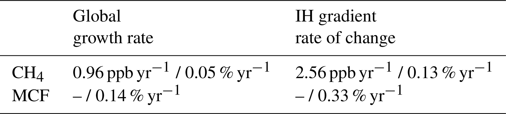
The hydroxyl radical (OH) is the main atmospheric oxidant and the primary sink of the greenhouse gas CH4. In an attempt to constrain atmospheric levels of OH, two recent studies combined a tropospheric two-box model with hemispheric-mean observations of methyl chloroform (MCF) and CH4. These studies reached different conclusions concerning the most likely explanation of the renewed CH4 growth rate, which reflects the uncertain and underdetermined nature of the problem. Here, we investigated how the use of a tropospheric two-box model can affect the derived constraints on OH due to simplifying assumptions inherent to a two-box model. To this end, we derived species- and time-dependent quantities from a full 3-D transport model to drive two-box model simulations. Furthermore, we quantified differences between the 3-D simulated tropospheric burden and the burden seen by the surface measurement network of the National Oceanic and Atmospheric Administration (NOAA). Compared to commonly used parameters in two-box models, we found significant deviations in the magnitude and time-dependence of the interhemispheric exchange rate, exposure to OH, and stratospheric loss rate. For MCF these deviations can be large due to changes in the balance of its sources and sinks over time. We also found that changes in the yearly averaged tropospheric burden of CH4 and MCF can be obtained within 0.96 ppb yr−1 and 0.14 % yr−1 by the NOAA surface network, but that substantial systematic biases exist in the interhemispheric mixing ratio gradients that are input to two-box model inversions.
To investigate the impact of the identified biases on constraints on OH, we accounted for these biases in a two-box model inversion of MCF and CH4. We found that the sensitivity of interannual OH anomalies to the biases is modest (1 %–2 %), relative to the uncertainties on derived OH (3 %–4 %). However, in an inversion where we implemented all four bias corrections simultaneously, we found a shift to a positive trend in OH concentrations over the 1994–2015 period, compared to the standard inversion. Moreover, the absolute magnitude of derived global mean OH, and by extent, that of global CH4 emissions, was affected much more strongly by the bias corrections than their anomalies (∼10 %). Through our analysis, we identified and quantified limitations in the two-box model approach as well as an opportunity for full 3-D simulations to address these limitations. However, we also found that this derivation is an extensive and species-dependent exercise and that the biases were not always entirely resolvable. In future attempts to improve constraints on the atmospheric oxidative capacity through the use of simple models, a crucial first step is to consider and account for biases similar to those we have identified for the two-box model.
- Article
(1638 KB) - Full-text XML
-
Supplement
(2024 KB) - BibTeX
- EndNote


For the interpretation of atmospheric observations in the context of, for example, atmospheric pollution or in that of global warming, atmospheric models are often used. Atmospheric models vary in complexity from simple one-box models to state-of-the-art 3-D transport models. Different types of models are suitable for addressing different types of problems to different degrees of scrutiny. Therefore, there is no model category that fits all problems. Simple box models are easy to set up, computationally cheap, and transparent. For these and other reasons, their use in atmospheric studies is ubiquitous and has provided useful insights (e.g. Quay et al., 1999; Walker et al., 2000; Montzka et al., 2011; Schaefer et al., 2016; Schwietzke et al., 2016). However, simple box models also put limitations on the derived results, as they are by definition less comprehensive than complex models. For example, box models do not explicitly contain much information on a species' spatial distribution, which can be important if interacting quantities (e.g. loss processes) are distributed non-homogeneously in space. Where exactly these limitations lie and what the gain is from increasing model complexity can be difficult to diagnose and depends on the application.
A problem that has often been approached in box models is that of constraining the global atmospheric oxidizing capacity, which is largely determined by the tropospheric hydroxyl radical (OH) concentration (Montzka et al., 2000, 2011). OH is dubbed the detergent of the atmosphere for its dominant role in the removal of a wide variety of pollutants, including urban pollutants (CO, NOx), greenhouse gases (CH4, HFCs), and HCFCs, which are greenhouse gases, and also contribute to stratospheric ozone depletion. The budgets of many of these pollutants have been strongly perturbed since pre-industrial times, and it is important to understand what consequences this has had in the past, and could have in the future, for the atmosphere's oxidizing capacity.
Due to its high reactivity, OH has a lifetime of seconds, which inhibits extrapolation of direct measurements. Moreover, OH abundance is the net result of many different reactions and reaction cycles, and thus modelling it process-based in full-chemistry models is complex and dependent on uncertain emission inventories of the many gases involved. Therefore, the most robust observational constraints on OH on the larger scales are thought to be derived indirectly from its effect on tracers: gases that are predominantly removed by OH. Depending on how well the tracer emissions are known, the time evolution of the global mixing ratio of such a tracer can serve to constrain OH. The most well-established tracer for this purpose is methyl chloroform (MCF; e.g. Montzka et al., 2000; Bousquet et al., 2005). In part, this is because it was identified early on as a tracer with a well-defined production inventory that allowed emission estimates with small errors, relative to other gases (Lovelock, 1977; Prinn et al., 1987). Moreover, production of MCF was phased out in compliance with the Montreal Protocol, and the resulting rapid drop in emissions made loss against OH the dominant term in the MCF budget (Montzka et al., 2011).
Research and debate surrounding OH (Krol and Lelieveld, 2003; Krol et al., 2003; Reimann et al., 2005; Prinn et al., 2005; Rigby et al., 2013; McNorton et al., 2016) has lead to considerable improvements in its constraints, for example, a likely upper bound on global interannual variability of OH of a few percent (Montzka et al., 2011). Two recent studies derived OH variations in a tropospheric two-box model through an inversion of atmospheric MCF and CH4 observations (Rigby et al., 2017; Turner et al., 2017). In such an inversion, a range of parameters is optimized (most prominently emissions of MCF and CH4 and OH) so that the modelled mixing ratios best match atmospheric observations of the tracers involved.
Both studies found that constraints on OH in this set-up were weak enough that a wide range of OH concentration variations over time and, by extent, CH4 emission scenarios were possible as an explanation for the post-2007 increase in its measured global mole fraction. This is an important conclusion, because the CH4 growth rate, combined with the CH4 lifetime (in turn dominated by MCF-derived OH), is generally assumed to provide the strongest top-down constraints on global CH4 emissions and variations therein. We note that in Rigby et al. (2017) the two tropospheric boxes were supplemented by a single stratospheric box, making it technically a three-box model. However, due to our focus on the troposphere, we hereafter treat this type of model, too, as a two-box model, and where relevant we discuss the implication of the addition of a stratospheric box.
There are two important reasons to approach the problem of constraining OH in a model of exactly two tropospheric boxes. Firstly, through the focus on annual timescales and hemispheric spatial scales, the result is only sensitive to interannual variability in large-scale transport of the modelled tracers. Moreover, by focusing on interannual variability as opposed to absolute OH or emission levels, remaining systematic offsets are not thought to significantly affect the outcome.
Secondly, a crucial part of the optimization consists of disentangling the influence of OH and that of emission variations on observed MCF mixing ratios. Ideally, MCF emission variations would be prior knowledge. However, though MCF production is well documented, the emission timing is much more uncertain (McCulloch and Midgley, 2001). MCF was mainly used as a solvent in, for example, paint and degreasers of metals. In these applications, MCF is released only when used, rather than when produced, which results in uncertainty in the emission timing. Moreover, due to the continuing decline of the atmospheric MCF mixing ratios, small, ongoing MCF emissions could eventually become important. Observation-inferred emissions exceeding bottom-up emission inventories have been identified both from the US (Millet and Goldstein, 2004) and from Europe (Krol et al., 2003) as well as from other processes, such as MCF re-release from the ocean (Wennberg et al., 2004). Therefore, in the absence of other constraints, emission uncertainties would limit the use of MCF for deriving interannual variability of OH. However, in a two-box set-up, an additional constraint is provided by the IH mole fraction gradient of MCF. Emission inventories show that MCF emissions are predominantly located in the Northern Hemisphere (NH), whereas OH has a NH to SH ratio that is uncertain, but the ratio has a likely range of 0.80 to 1.10 (Montzka et al., 2000; Patra et al., 2014). This means that emission variations have a strong effect on the IH mole fraction gradient of MCF, whereas the effect of large-scale OH variations is much weaker. Thus, the IH gradient is an important piece of information that can help to disentangle the influence of emissions from the influence of OH on MCF growth rate variations. This use of the IH gradient for constraining global emissions of anthropogenically emitted gases has also been recognized in previous research (Liang et al., 2017; Montzka et al., 2018).
Despite the appealing degree of simplicity offered by the two-box model, its results still hinge on many simplifying assumptions, both explicit (e.g. interhemispheric transport) and implicit (e.g. intrahemispheric transport). In this context, the uncertain outcome of the two recent two-box model studies puts forward an important question: how do the simplifying assumptions inherent to the two-box set-up affect the conclusions drawn from it? Or, conversely, would these conclusions change when moving the analysis to a 3-D transport model? A recent study (Liang et al., 2017) partly explored these questions. The study investigated how to incorporate information from 3-D transport models in a two-box model to increase the robustness of two-box model-derived constraints on OH. They found that there are key parameters in the two-box model that can be tuned to better represent the 3-D simulation results and thus ideally better represent atmospheric transport in general. For example, they found that IH transport rates can be species-dependent.
Here, we provide a different approach to the issue. In the first part of our study, we parametrized results from the 3-D global transport and chemistry model TM5 into a two-box model. Through this parametrization, we explored difficulties in the translation from the “reality” of a 3-D transport model to a two-box model and the assumptions made in the process. We focused on four aspects of the parametrization.
Firstly, we investigated the tracer-dependent nature of IH transport as reported by Liang et al. (2017). Secondly, we analysed the IH OH ratio. Previous research has shown that because of tracer-specific source–sink distributions, different tracers can be exposed to different global mean OH concentrations (Lawrence et al., 2001). We extended this observation to a species-dependent IH OH ratio. Thirdly, we looked at the stratospheric loss for MCF specifically. This net loss to the stratosphere might be slowing after its emissions dropped (Krol and Lelieveld, 2003; Bousquet et al., 2005). Fourthly, we used the 3-D simulation to investigate differences between the burden seen by the surface measurement network of the National Oceanic and Atmospheric Administration Global Monitoring Division (NOAA-GMD) and the true tropospheric and hemispheric burden in our 3-D model, a bias that was also discussed in Liang et al. (2017).
In the second part of this study, we assessed the impact of these four potential biases on derived OH variations in a two-box inversion set-up that is very similar to Rigby et al. (2017) and Turner et al. (2017). The objective was to provide a quantitative estimate of the impact of biases in a two-box inversion and to explore if and how these can be accounted for. Though this study is focused on the problem of OH, it also serves as a case study of potential pitfalls in two-box models in general, when applied to interpreting global-scale atmospheric observations.
2.1 Two-box inversion
In this section, we discuss the set-up of our two-box model inversion. The model incorporated two tracers (MCF and CH4) and consisted of two boxes (the troposphere in the NH and in the SH), which were delineated by the Equator, i.e. it is fixed in time. The stratosphere was implicitly included in the model through a first-order loss process that was taken to be equal for both hemispheres. The governing equations for a tracer mixing ratio X are given in Eq. (1).
Thus, within each hemisphere, there were emissions (E), loss to OH (kOH[OH]X), loss to the stratosphere (lstratX), loss to other processes (lotherX; e.g. ocean deposition), and transport between the hemispheres (kIH(XNH−XSH)). The model ran at an annual time step. The fundamentals of this model set-up are also found in Rigby et al. (2017) and Turner et al. (2017), though the exact treatment of the different budget terms can differ. For example, Turner et al. (2017) combined all tropospheric loss, including loss to the stratosphere, in one term, whereas Rigby et al. (2017) included a stratospheric box, so that stratospheric loss becomes a transport rather than a first-order loss term. Where relevant, we point out further differences with these previous studies.
Since the objective was to leverage observed mixing ratios to infer information on tropospheric OH, we also set up an inverse estimation framework, complementary to the above forward model. The objective of the inversion was to optimize a state x, such that the forward model best reproduced the observations without straying too far from a first best guess: the prior. Therefore, the state is the vector which contains all parameters that needed to be optimized. The optimization objective is analogous to minimizing the cost function J, as defined in Eq. (2):
when B and R are the prior and observation error covariance matrices respectively, H is the forward model, and y is the observation vector. In addition, we compute the cost function gradient ∇J (Eq. 3).
with HT the transpose of the forward model, also known as the adjoint model. Note that because the forward model H was non-linear (e.g. OH chemistry), we used the adjoint of the tangent-linear forward model. Calculation of the cost function gradient facilitates quicker convergence of the optimization. For the minimization we used the Broyden–Fletcher–Goldfarb–Shanno algorithm. In essence, this statistical inversion set-up is the same as that used in the 4DVAR system of ECMWF (Fisher, 1995) and TM5-4DVAR (Meirink et al., 2008).
For the optimization of MCF emissions, we used an extended version of the emission model from McCulloch and Midgley (2001). This emission model was adopted to account for the varying and uncertain release rates of MCF when used in different applications (e.g. degreasing agent or paint). This uncertainty results in a gap between the uncertainty in production, or integrated emissions (∼2 %), and the uncertainty in annual emissions (McCulloch and Midgley, 2001). Therefore, production was distributed between four different categories with different release rates: rapid, medium, slow, and stockpile. In the prior distribution, the bulk of production (>95 %) was placed in the rapid category. To account for uncertainty in the production inventory, we also adopted an additional emission term superimposed on the production-derived emissions. The emissions in year i were then given by Eqs. (4) and (5). For each year i, we optimized four parameters for MCF emissions: three parameters that shifted emissions between the rapid production category and each of the other three categories (, , and in Eq. 6) and the additional emissions term (), which had an uncertainty constant through time. This emission model is similar to that used in Rigby et al. (2017), though ours leaves more freedom with respect to the timing of emissions.
for the emissions in year i, where
and, in the optimization,
An important choice in the inversion set-up is which parameters to prescribe and which to optimize. Rigby et al. (2017) optimized all parameters, so as to explore the full uncertainty of the optimization within the inversion framework. Turner et al. (2017) only optimized hemispheric MCF and CH4 emissions and hemispheric OH, while the remaining uncertainties were partly explored in sensitivity tests. We choose to optimize four end products for each year: global OH, global MCF emissions, global CH4 emissions, and the CH4 emission fraction in the NH. Thus we had a closed system, as we also fitted to four observations: the global mean mixing ratio and the IH gradient of both MCF and CH4. In addition to the 4DVAR inversion, we generated a Monte Carlo ensemble, where in each realization, the prior and the observations were perturbed, relative to their respective uncertainties. Then, the new prior was optimized using the new observations. The Monte Carlo simulation quantified the sensitivity of the optimization to the prior choice and to the realization of the observations. The Monte Carlo set-up also allowed us to explore the sensitivity of the inversion to parameters that were not optimized, such as the fraction of MCF emissions in the NH. This approach had the added advantage that parameters that were perturbed in the Monte Carlo simulation, but not optimized in the 4DVAR system, did not need to have a Gaussian error distribution. Gaussian probability distributions are normally a prerequisite in a 4DVAR inversion. The specifics of our inversion set-up are given in Table 1.
McCulloch and Midgley (2001)Table 1The relevant settings we used in the inversion of our two-box model. The upper section contains the parameters optimized in the inversion, which were also perturbed in the Monte Carlo ensemble. These parameters have Gaussian uncertainties, and their mean and 1σ uncertainty are given. The middle section contains parameters that were perturbed in the Monte Carlo, but not optimized. The middle parameters have uniform uncertainties, of which the lower and upper bound are given. The bottom section contains parameters that were neither optimized nor perturbed. For these parameters, the left column gives the standard setting, whereas the alternative column indicates whether we also ran an inversion using a TM5-derived time series (see Sect. 2.2.2).
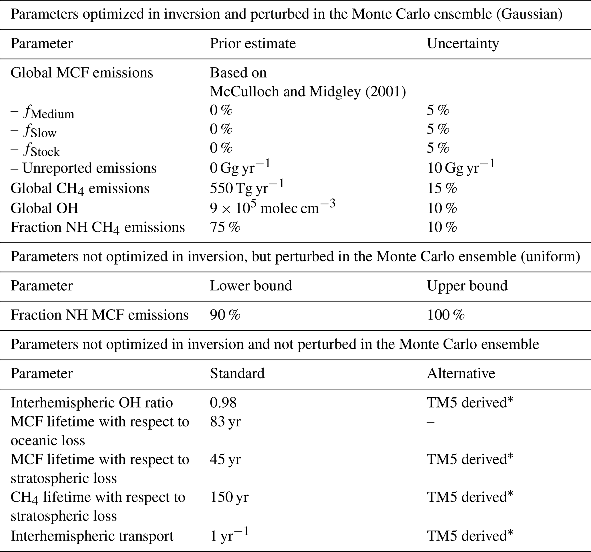
*see Sect. 2.2.2.
2.2 TM5 set-up and two-box parametrizations
2.2.1 3-D model set-up
For the 3-D model simulations we used the atmospheric transport model TM5 (Krol et al., 2005). The model was operated at a horizontal resolution, at 25 vertical hybrid sigma-pressure levels. The simulation period was 1988–2015, where we treated 1988 and 1989 as spin-up years. TM5 transport was driven by meteorological fields from the ECMWF ERA-Interim reanalysis (Dee et al., 2011). Convection of tracer mass was based on the entrainment and detrainment rates from the ERA-Interim dataset. This is an update from the previous convective parametrization used by, for example, Patra et al. (2011). The new convective scheme results in faster interhemispheric exchange of tracer mass, more in line with observations (Tsuruta et al., 2017).
We ran TM5 with three tracers: CH4, MCF, and SF6. For CH4, we annually repeated the 2009–2010 a priori emission fields used by Pandey et al. (2016), and we also used the same fields for stratospheric loss to Cl and O(1D). For MCF, we used emissions from the TransCom-CH4 project (Patra et al., 2011). Since these emissions were available only up to 2006, we assumed a globally uniform exponential decay of 20 % yr−1 afterwards, similar to Montzka et al. (2011). MCF-specific loss fields (ocean deposition and stratospheric photolysis) were also taken from the TransCom-CH4 project. Details of the MCF loss and emission fields can be found in the TransCom-CH4 protocol (http://transcom.project.asu.edu/pdf/transcom/T4.methane.protocol_v7.pdf, last access: 1 September 2018). The OH loss fields we used were a combination of the 3-D fields from Spivakovsky et al. (2000) in the troposphere and stratospheric OH as derived using the 2-D MPIC chemistry model (Brühl and Crutzen, 1993). The OH fields were scaled by a factor 0.92, as described by Huijnen et al. (2010). For SF6, we used emission fields from the TransCom Age of Air project (Krol et al., 2018), with no loss process implemented.
Since the above set-up is simplistic in some aspects (e.g. annually repeating CH4 emissions), we also ran a “nudged” simulation. In the nudged simulation, we scaled the mixing ratios of a tracer up or down in latitudinal bands, depending on the mismatch of the model with NOAA observations (analogous to Bândă et al., 2015), with a relaxation time of 30 days. This method ensured that the model followed the long-term trend in observations without requiring a full inversion. The nudged simulation provided a test of the sensitivity of our results to the source–sink distributions we used in the 3-D simulation.
2.2.2 Parametrizing 3-D model output to two-box model input
Here we outline how we used the TM5 simulations to derive two-box model parametrizations for stratospheric loss (lstrat) and for interhemispheric exchange (kIH). Firstly, the 3-D fields were divided into three boxes: the troposphere in the NH and in the SH and the stratosphere. The border between the hemispheres was taken as the Equator, fixed in time. Where relevant we discuss the sensitivity of our results to this demarcation. We defined a dynamical tropopause as the lowest altitude where the vertical temperature (T) gradient is smaller than 2 K km−1, clipped at a geopotential height of 9 and 18 km. Our analysis was found to be insensitive to the exact definition of the tropopause. Next, we computed an annual budget for each box. For the two tropospheric boxes, this was done as in Eq. (1). This was supplemented by Eq. (7) for the stratospheric box.
where emissions, local loss, and mixing ratios per box could be derived from the 3-D model in- and output, and thus lstrat and kIH could be inferred from these equations. Note that we did not strictly need the stratospheric budget equation to resolve two parameters, but we used it to resolve numerical inaccuracies. Resolving the budget of each species in this manner provided the necessary input of the tropospheric two-box model defined in Sect. 2.1 such that on the hemispheric and annual scale, identical results were obtained with the 3-D and the two-box models.
An additional parameter that we derived from the TM5 simulations was the IH OH ratio to which each tracer was exposed. We quantified this parameter as the ratio between hemispheric lifetimes with respect to OH (τOH):
Note that this ratio might differ from the physical IH OH ratio because of correlations between the tracer distribution, the OH field, and the temperature distribution.
2.2.3 Model-sampled observations
The standard in tracking global trends in atmospheric trace gases are surface measurement networks. For CH4 and MCF these are most notably the NOAA-GMD (Dlugokencky et al., 2009; Montzka et al., 2011) and the AGAGE (Prinn et al., 2018) networks. By selecting measurement sites far removed from sources, the theory is that a small number of sites already puts strong constraints on the global growth rate (Dlugokencky et al., 1994). In general, quantification of the robustness of the derived growth rates based solely on observations can be difficult, since there are likely systematic biases inherent to sampling a small number of surface sites. When assimilated into a 3-D transport model, these biases will largely be resolved (if transport is correctly simulated). However, when the data are aggregated to two hemispheric averages, as in a two-box model, quantification of the potential biases is crucial.
We explored the resulting bias in our model framework. By subsampling the TM5 output at the locations of NOAA stations, at NOAA measurement instances, we generated a set of model-sampled observations. These model-sampled observations were intended to be as representative as possible for the real-world observations of the NOAA network. To aggregate the station data to hemispheric averages, we used methods similar to those deployed by NOAA (for MCF, Montzka et al., 2011, with further details on our adaption in Sect. S1 in the Supplement; for CH4, Dlugokencky et al., 1994). Hemispheric averages for CH4 were derived from 27 sites and MCF averages from 12 sites. By comparison of the resulting products with the calculated tropospheric burden, as derived from the full tropospheric mixing ratios, we could assess how well the burden derived from the NOAA network represents the model-simulated tropospheric burden. The two end products we investigated for each tracer were the rate of change of the global mean mixing ratio and that of the IH gradient. Note that by mixing ratio we mean the dry air mole fraction. These two parameters best reflect the information as it is used in a two-box model; the global mean mixing ratio is used to constrain the combined effect of OH and emissions, while the IH gradient is used to distinguish between the two. Note that in previous box-model studies of MCF, often only global growth rates were derived (Montzka et al., 2000, 2011).
2.3 Potential biases in the two-box model
By concentrating on the budget of MCF, we identified three parameters that need attention in the two-box model: IH transport, the IH OH ratio, and loss of MCF to the stratosphere. In addition, we investigated the potential bias in converting station data to hemispheric averages (see Sect. 2.2.3 and S1). We quantified these biases and propagated them in two-box model inversions, as discussed in Sect. 3.2, to quantify their impact on derived quantities related to OH.
Interhemispheric transport
IH transport of tracer mass can vary because of variations in IH transport of air mass (e.g. influenced by the El Niño–Southern Oscillation, particularly at Earth's surface; Prinn et al., 1992; Francey and Frederiksen, 2016; Pandey et al., 2017) or because of variations in the source–sink distribution and thus of the tracer's concentration distribution itself. Generally, interannual variability in IH transport is considered to be on the order of 10 % (Patra et al., 2011). Two-box model studies typically assume time-invariant IH exchange (Turner et al., 2017) and/or similar exchange rates for different tracers (Rigby et al., 2017). Here we investigated whether such assumptions hold for a tracer which undergoes strong source–sink redistributions over time, such as MCF. The IH transport variations we derived for each tracer are discussed in Sect. 3.1.1.
Surface sampling bias
As discussed in Sect. 2.2.3, we explored the bias that results from representing hemispheric averages using sparse surface observations. Surface networks are a valuable resource, because they provide high-quality, long-term measurements of a growing variety of tracers. However, temporal, horizontal, and vertical coverage of surface networks is limited. In Sect. 3.1.2 we discuss how these limitations can result in biases in two-box model observations.
The interhemispheric OH ratio
The IH ratio of OH concentrations is an uncertain parameter. This is mostly because of a mismatch between results from full-chemistry models (1.13–1.42; Naik et al., 2013) and from MCF-derived constraints (0.80–1.10; Brenninkmeijer et al., 1992; Montzka et al., 2000; Patra et al., 2014). The latter is generally the loss ratio considered in two-box models (1.0 in Turner et al., 2017, and 0.95–1.20 in Rigby et al., 2017) and is similar to the ratio we used in the TM5 simulations (0.98 Spivakovsky et al., 2000). However, the bias we consider here is of a different nature; it is the difference between the physical IH OH ratio and the IH loss ratio a particular tracer is exposed to. It is known that different tracers can be exposed to different oxidative capacities (Lawrence et al., 2001). Therefore, different tracers might similarly be influenced by different IH ratios in OH. We explore this bias in Sect. 3.1.3.
MCF loss to the stratosphere
The second-most important loss process of MCF is stratospheric photolysis. In our TM5 set-up, this loss process resulted in an in-stratosphere lifetime (stratospheric burden divided by stratospheric loss) of 4 to 5 years. It is generally assumed that this in-stratosphere loss translates to a global lifetime of MCF with respect to the stratosphere (global burden divided by stratospheric loss) of 40 to 50 years (Naik et al., 2000; Chipperfield and Liang, 2013), which corresponds to ∼10 % of global MCF loss. Rigby et al., 2017 assumed a time-invariant in-stratosphere lifetime, but due to the inclusion of a stratospheric box, the global lifetime with respect to stratospheric loss could vary somewhat due to changes in the troposphere–stratosphere gradient. These variations were tuned to result in a global lifetime with respect to stratospheric loss of 40 (29–63) years. Turner et al. (2017) incorporated this loss process in the OH loss term. Due to the rapid drop in MCF emissions and the relatively slow nature of troposphere–stratosphere exchange, this lifetime could vary through time (Montzka et al., 2000; Krol and Lelieveld, 2003; Bousquet et al., 2005). We will investigate this possibility in Sect. 3.1.4.
2.4 Standard two-box inversion and bias correction
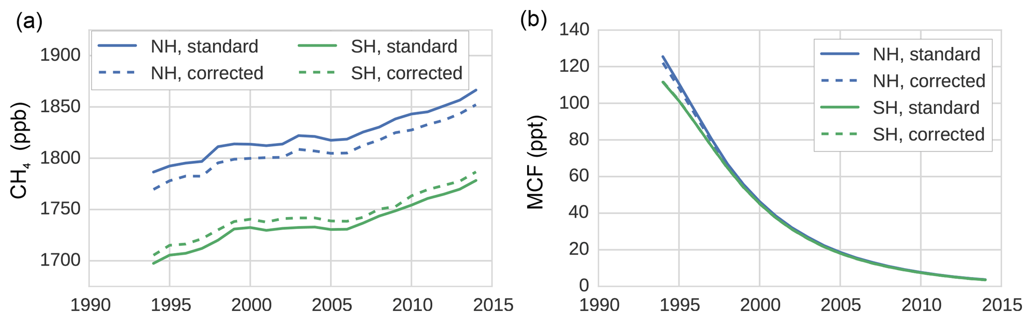
Figure 1Hemispheric, annual mean time series of CH4 (a) and MCF (b), as derived from the NOAA surface sampling network (for CH4, 27 sites were used; for MCF, 12 sites were used). Solid lines denote averages as derived directly from the NOAA surface sampling network (which are used in our standard inversion). Dashed lines denote the same time series, but those that are adjusted by correction factors that were derived from our TM5 simulations. The correction factors reflect the differences between hemispheric averages based on model-sampled observations and hemispheric averages derived from the full TM5 troposphere. Figure 3 shows the ratios between the standard and corrected time series.
To assess the impact of the biases discussed in Sect. 2.3 on a two-box model inversion, we ran our inversion (see Sect. 2.1) using different settings. In the standard, default inversion, we did not consider any of the four biases discussed above. Thus, we used constant IH exchange (1 year), constant stratospheric loss of MCF (45 years), and a constant IH OH ratio (0.98; see Table 1). The first three potential bias corrections were then straightforwardly implemented by replacing these constant values with the time series we derived for each parameter from the full 3-D simulations (details in Sect. 2.2.2). As mentioned in Sect. 2.1, the inversion did not include uncertainties in these three parameters. We did this because conventional uncertainties tend to be large, therefore including them would have attenuated the impact of the bias corrections, while the corrections were the main interest of this comparison. For the surface sampling bias, we first computed a correction between the hemispheric means as derived from the model-sampled observations and the calculated (TM5) hemispheric, tropospheric means (with demarcation at the Equator). Then, we applied this correction to the real-world NOAA hemispheric means we used in the standard inversion. This gave a new set of observations, which we used in the inversion (discussed in Sect. 3.1.2). Both the standard and the corrected set of observations are shown in Fig. 1. Through comparison of the results of the standard inversion and of an inversion with one or more biases implemented simultaneously, we can evaluate the individual and cumulative impact of the biases on derived OH and CH4 emissions.
3.1 Biases
3.1.1 Interhemispheric transport

Figure 2The IH exchange rate for MCF, CH4, and SF6, as derived from a TM5 simulation (see Sect. 2.2.2).
The IH exchange coefficients, derived for the three different tracers as described in Sect. 2.2.2, are shown in Fig. 2. Clearly, the exchange rates differ between tracers both in mean value as well as in interannual variability. MCF is the clear outlier, but SF6 and CH4 also show different variations. The drivers of these differences are differences in intrahemispheric tracer distributions and in the underlying source and sink distributions. The three tracers differ strongly in this respect; SF6 and MCF are emitted almost exclusively in the NH mid-latitudes, whereas CH4 has significant emissions in the tropics and in the SH. SF6 has no sink implemented in our simulations, whereas MCF and CH4 have a sink with a distinct tropical maximum in OH. This all affects how IH transport of air mass translates to IH transport of tracer mass.
Most notable is the minimum in the IH exchange rate for MCF in the 2000–2005 period. The timing of the 1989–2003 decline in kIH coincides with the initial drop in MCF emissions. An important shift in the distribution of the MCF mixing ratio is that the global minimum shifts from the South Pole to the tropics. In the same period, there is a strong vertical redistribution which has also likely impacted IH exchange. It is not obvious that these changes should result in slower IH exchange, but in the end, in TM5, they do.
Another notable feature is the positive trend in the IH exchange rate for CH4 ( % yr−1; p=0.00) and for SF6 ( % yr−1; p=0.00). For CH4, we used annually repeating sources, whereas for SF6 we included emission variations (see Sect. 2.2). This means that for CH4, changes in the source–sink distribution did not contribute to the trend or to the variability. Indeed, in a simulation with annually repeating meteorology, we found near-zero variability in kIH for CH4 (see Sect. S4). Therefore, there is something in the combination of the meteorological data, the treatment of this data in TM5, and the source–sink distribution of both CH4 and SF6 which resulted in a significantly positive trend in the IH exchange rate of both gases. This trend could either indicate an acceleration of IH transport of air mass or a shift in the pattern of IH transport which favours IH exchange of CH4 and SF6. It is unclear from this analysis what the underlying mechanism is exactly, except that it is driven by temporal variations in transport, thus there are parameters in the meteorological fields which also show a trend; otherwise this final product cannot exhibit a trend. However, it might be that the sensitivity of TM5 transport to these parameters is biased.
To test the sensitivity of the derived IH exchange rates to the source–sink distribution, we compared kIH derived from the standard simulation to the nudged simulation (the nudging procedure is explained in Sect. S2). IH transport of CH4 as derived from the nudged simulation showed higher interannual variations than in the standard simulation (more discussion in Sect. S4), which can be expected, as the source–sink distribution becomes more variable. However, the general characteristics were conserved; most notably, the positive trend over the entire period persisted, for CH4 and for SF6. For MCF, we find that the general characteristics of derived kIH are similarly insensitive to nudging, with the main change being a deeper 2000–2005 minimum in the nudged simulation. In the end, we deem the anomalies presented in Fig. 2 to be quite robust with respect to the spatio-temporal source–sink distribution.
When the hemispheric interface is shifted from the Equator to 8∘ N, which is more representative of the average position of the Intertropical Convergence Zone (ITCZ), the IH exchange rate increases for all tracers, but the variability in IH exchange of CH4 and SF6 remains largely unaffected (see Sect. S4). However, for MCF, the variability shifts completely. Rather than decreasing after the emission drop, the IH exchange rate now increases. This sensitivity reflects that for a tracer with a relatively small IH gradient which minimizes in the tropics, it becomes difficult to define an IH transport rate in a two-box model. By extension, care should be taken when interpreting the IH gradient of MCF in later years, since the influence of IH transport is difficult to isolate. Sensitivities in the derivation of the IH exchange rate are discussed in more detail in Sect. S4.
3.1.2 Surface sampling bias
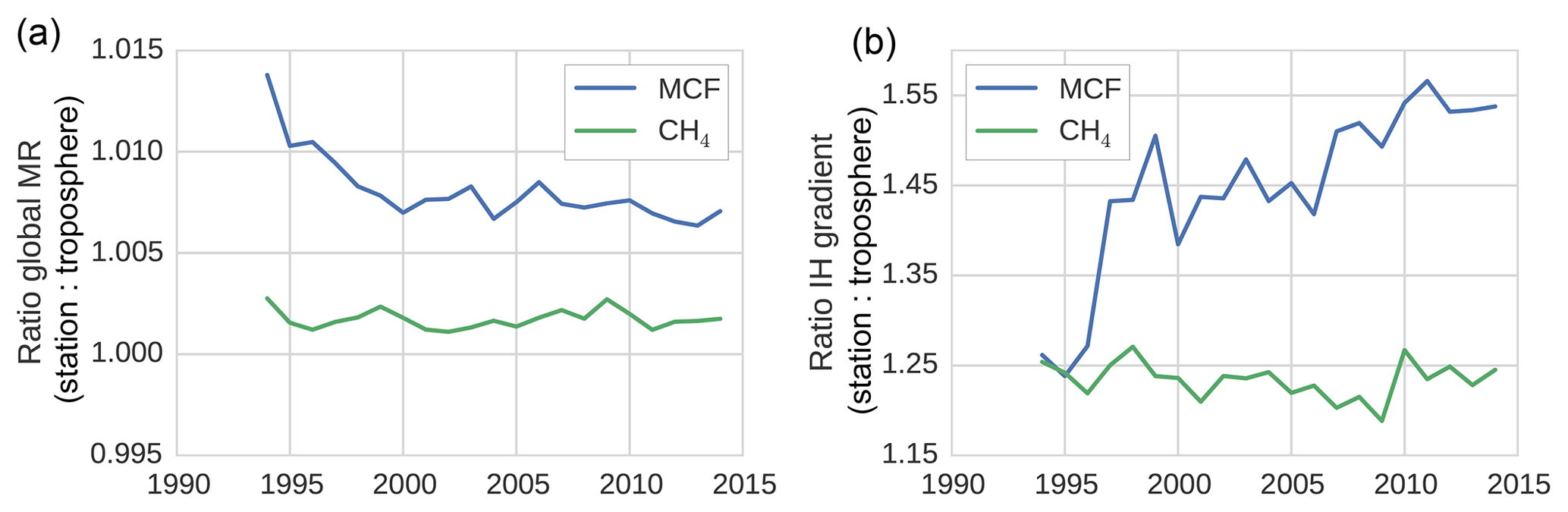
Figure 3The surface sampling bias in the global mixing ratio (MR) (a) and in the IH gradient (b) of MCF and of CH4. The bias was quantified as the ratio between values derived from the NOAA surface sampling network and values derived from the full (TM5) troposphere. The biases were derived from 27 and 12 sites for CH4 and for MCF, respectively. Figure 1 visualizes the impact of correcting for the sampling bias in real-world NOAA observations.
Table 2Mean observational errors as derived from TM5 simulations over the 1994–2015 period. The errors were quantified as the mean difference between annual means derived from model-sampled observations and annual means derived from the full tropospheric grid. CH4 uncertainties are given both in ppb yr−1 and relative to the global mean mixing ratio. Uncertainties for MCF are only given relative to the global mean because of its strong temporal decline.
Figures 1 and 3 show the surface network bias in the global mean mixing ratios and in the IH gradient. In Fig. 3, the bias is quantified as the ratio between values derived from the model-sampled observations (see Sect. 2.2.3) and values derived from the hemispheric (TM5) troposphere. A comparison with global mean mixing ratios derived from real-world NOAA observations is given in Sect. S2.
The bias in the IH gradient was particularly large, because averages based on NOAA surface stations systematically overestimated the tropospheric burden in the NH and underestimated the burden in the SH. Two important effects contributed to this bias. Firstly, in the NH, where most emissions were located, mixing ratios tended to decrease with altitude, while in the SH vertical gradients were much smaller or even reversed. Secondly, latitudinal gradients of both MCF and CH4 tended to be highest in the tropics, where few or no measurement sites were available. Again, due to high emissions in the NH, mixing ratios in the NH decreased towards the Equator, while mixing ratios increased towards the Equator in the SH. Both biases were of the opposite sign in each hemisphere. Thus, in a global average, these biases largely cancelled, and only a small overestimate remained (Fig. 3a). For the IH gradient, however, these biases added up, which resulted in an overestimate of the IH gradient by surface stations of up to 20 %–40 % (Fig. 3b). For MCF before 1995 and for CH4 throughout the analysis period, the bias from the vertical gradient dominated. The shift in the bias for MCF was driven by a shift in the latitudinal gradient. The IH gradient of MCF got a minimum in the tropics, and apparently this exacerbated the effect of the lack of tropical stations, combined with the simple, linear latitudinal interpolation we adopted for MCF (see Sect. S1).
We note that the derived bias in the IH gradient is sensitive to the demarcation of the two tropospheric boxes. When we shifted the IH interface from the Equator to 8∘ N, the bias was reduced to 15 % for CH4 and varied between 15 % and 25 % for MCF. The trend in the IH bias of MCF became smaller but persisted.
Liang et al. (2017) performed a similar analysis for MCF. They reported a similar low-to-absent bias in the global mean and a more significant bias in the IH gradient of MCF (∼10 %). This is smaller than the bias we found, even if we demarcated the hemisphere at 8∘ N. However, an important difference is that in Liang et al. (2017), model-sampled observations were compared to the surface grid, instead of to the full troposphere. Thus, their bias estimate did not include vertical effects. When we used the surface grid as a reference, the IH bias for CH4 was reduced to −10 %, i.e. it reversed. For MCF the bias shift persisted, and the maximum bias was only slightly reduced to 15 %, indicating a dominant influence from the latitudinal dimension. We emphasize that for a tropospheric two-box model, the comparison with the full troposphere is most relevant.
This analysis also provided an estimate of uncertainties in the rate of change of the global mixing ratio and in that of the IH gradient: the relevant observational parameters in a two-box inversion. Table 2 gives the differences between the quantities derived from model-sampled observations and from the full troposphere, i.e. the “true” (TM5) error. We can compare this TM5-derived uncertainty to uncertainties derived only from observations, which we used in the two-box inversions. For CH4, we used uncertainties as reported by NOAA. These were obtained by generating an ensemble of surface network realizations, where in each realization different sites are excluded or double-counted randomly (bootstrapping). For each realization, aggregated quantities such as the global mean growth rate can be derived. The spread within the ensemble then provides a measure for the uncertainty. For MCF no such uncertainties are reported. Therefore, we developed our own method, which is described in Sect. S1.
Following these methods, we found observation-derived uncertainties in the global mean growth rate of around 0.60 ppb yr−1 and 0.6 % yr−1 for CH4 and for MCF respectively. NOAA does not report an uncertainty in the IH gradient of CH4, but error propagation from hemispheric means gave an uncertainty of 1.1 ppb yr−1. For MCF, we found a time-dependent uncertainty in the rate of change of the IH gradient of 1.0 %–1.5 %.
The CH4 errors we derived from the TM5 simulation were slightly higher than the uncertainties reported by NOAA. Furthermore, since we used annually repeating CH4 emissions, variations in CH4 emissions can further increase the error. Indeed, the nudged run (see Sect. S2) resulted in 20 % higher uncertainties. However, it is important to note that the CH4 uncertainties reported by NOAA are intended to reflect the match with the marine boundary layer (MBL), rather than with the full troposphere. Therefore, it is not surprising that the errors we find are somewhat higher.
For MCF, we adopted observation-derived uncertainties that were significantly lower than those used by Rigby et al. (2017) and Turner et al. (2017); both studies reported uncertainties of around 5 % in hemispheric averages. Both studies used different methods that were grounded on different observational information. In Rigby et al. (2017), temporal variability dominated the uncertainty estimate, while in Turner et al. (2017) spatial variations were used. Our method is more similar to Rigby et al. (2017) but with modifications that averaged out some of the temporal variability, under the assumption that variability at different measurement sites was largely uncorrelated (details in Sect. S1). This shows that observation-derived uncertainties in MCF averages are uncertain quantities, in large part due to the relatively low number of available surface sites. Therefore, the uncertainty derived from TM5 is an especially useful addition for MCF.
Table 2 shows that TM5-derived uncertainties in MCF averages are significantly lower than all observation-derived estimates. This result indicates that even the use of a simple averaging algorithm and a small number of surface sites, relative to what is available for CH4, already results in well-constrained hemispheric and global growth rates for MCF. The TM5-derived estimate thus supports the use of our observation-derived uncertainty estimates, rather than the higher estimates used in previous studies.
3.1.3 Interhemispheric OH ratio
In the TM5 simulations from which the global loss rates were derived, the prescribed tropospheric OH fields were taken from Spivakovsky et al. (2000). In these fields, the IH OH ratio is 0.98 when the IH interface is considered to be the Equator. One might expect a similar ratio between OH loss in the NH and in the SH, which we quantified through the IH ratio in tracer lifetime with respect to OH loss (Eq. 8). We found that this is not the case (see Fig. 4).
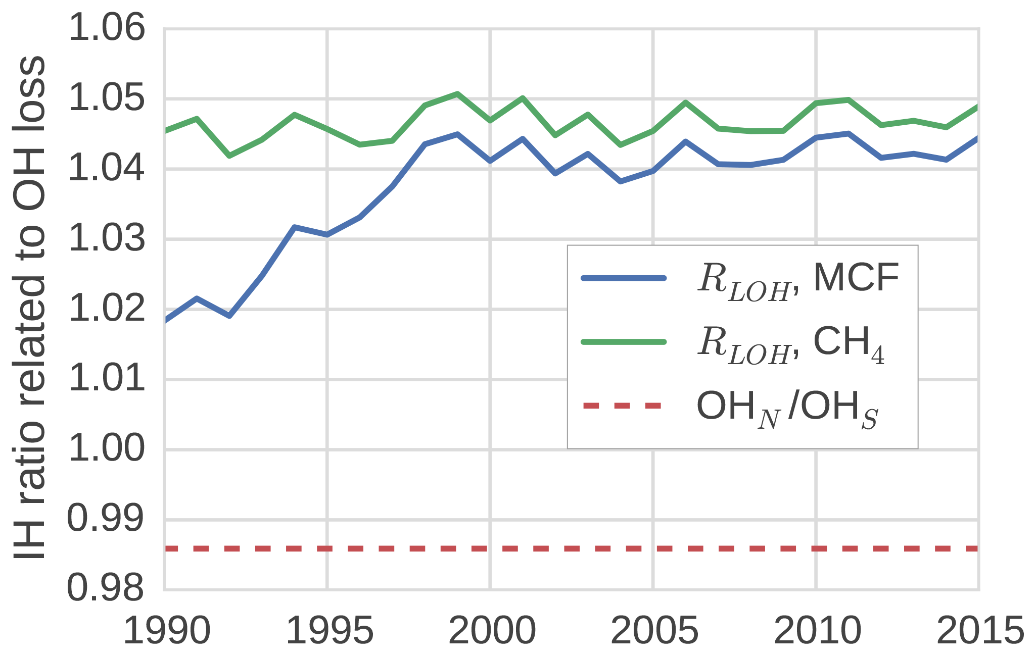
Figure 4The ratio between tracer lifetime with respect to OH loss in the SH troposphere and NH troposphere (see Eq. 8). Additionally, the IH ratio in OH concentrations is shown.
The loss ratio was up to 7 % higher than the physical OH ratio. Moreover, the ratio was not the same for MCF and CH4, and the ratio that corresponded to MCF showed a trend. The IH asymmetry in temperature in our model was small, so it did not explain the difference between the IH loss and the IH OH ratio. Instead, we found that the systematic positive offset was largely driven by an IH asymmetry in the spatio-temporal correlations between OH and temperature. Mostly, this was because the OH maximum in the NH was located at lower altitude than in the SH in our 3-D model. Since at low altitudes, temperatures are higher, and higher temperatures correspond to higher reaction rates, this asymmetry resulted in relatively high NH loss rates. As such, the ratio bias was sensitive to the OH distribution used in the 3-D model simulation.
The trend in the ratio for MCF was driven by the change in the spatial distribution of MCF after the emission drop in the mid-1990s. Before the drop, the IH gradient of MCF was emission-driven and high (25 %). This resulted in a negative correlation between OH ∕ temperature and MCF in the NH, which drove the initially lower loss ratio. After the emission drop, the IH gradient became largely sink-dominated and dropped to 3 %. The ratio then became similar, though not identical, to that of CH4, which also has a relatively low IH gradient (5 %). The exact reasons for the IH asymmetry in the OH loss rate were complex; further details are discussed in Sect. S3.
The derived IH OH ratio was sensitive to the demarcation of the two tropospheric boxes. When we shifted the position from the Equator to 8∘ N, all IH OH ratios were reduced by 10 % to 15 %. However, the offset between the physical IH OH ratio and the actual loss ratio remained similar, as did the trend in the loss ratio for MCF.
3.1.4 Loss to the stratosphere
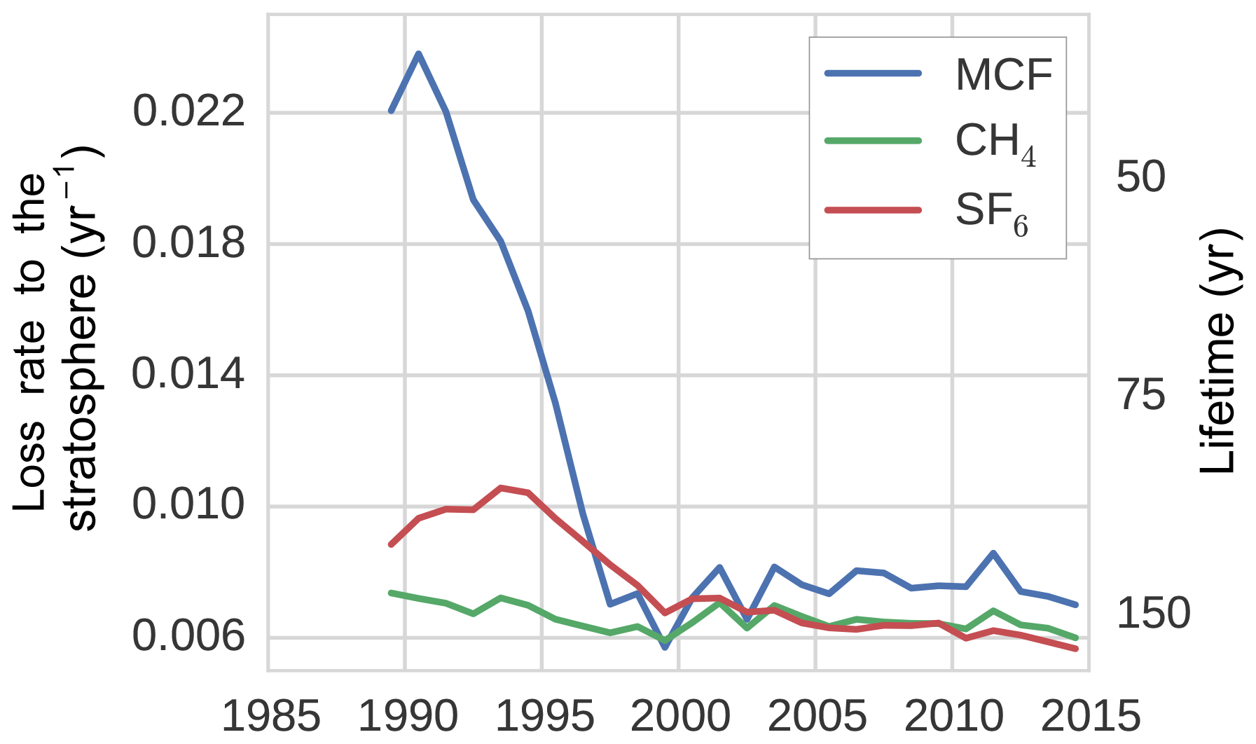
Figure 5The tropospheric loss rate to the stratosphere, as derived from the TM5 simulations (see Sect. 2.2.2).
Figure 5 shows the stratospheric loss rate, as derived from Eqs. (1) and (7). Most notably, the stratospheric loss rate showed a significant negative trend for MCF, decreasing by 68 % from 1991 to 1997. The lifetime of MCF with respect to stratospheric loss, as calculated from TM5, was in 1990 similar to the range reported in literature: 40 to 50 years (Naik et al., 2000; Chipperfield and Liang, 2013). Afterwards however, the corresponding timescale for stratospheric loss quickly increases. As loss to the stratosphere is a secondary loss process, it is generally assumed that variability in MCF loss is driven predominantly by OH variations (Montzka et al., 2011; Turner et al., 2017; Rigby et al., 2017). Here, we found that this is not necessarily the case. The decline in loss to the stratosphere was not an artefact resulting from treating a transport process as a loss process; when taking the exchange proportional to the troposphere–stratosphere gradient, we still found a decrease in the exchange rate of 63 %. Previous research has identified that the tropospheric lifetime with respect to stratospheric loss could be decreasing (Krol and Lelieveld, 2003; Prinn et al., 2005; Bousquet et al., 2005), but not to the degree that we found here and not relative to the troposphere–stratosphere gradient. This is important, because it means that a three-box model with an explicit stratospheric box, such as in Rigby et al. (2017), would also not capture the decline.
The explanation we suggest for the increase in MCF lifetime with respect to stratospheric loss has to do with the nature of troposphere–stratosphere exchange, which consists of an upward and a downward flux. In practice, as MCF emissions decreased, the troposphere started to transport air to the stratosphere which was exposed to lower MCF emissions, while the stratosphere was still transporting older air back to the troposphere (in the downward branch of the Brewer–Dobson circulation; Butchart, 2014) that was exposed to higher MCF emissions. Therefore, the delay between the two opposed fluxes resulted in a reduced net upward flux rate in an atmosphere with decreasing emissions compared to an atmosphere with increasing or constant emissions. Consistent with this hypothesis, we found that the stratospheric loss rate did not decrease in a TM5 simulation with MCF emissions fixed at 1988 levels and that stratospheric loss did decrease, but recovered, when we fixed emissions at 2005 levels over the entire analysis period (results not shown). This also implies that the troposphere–stratosphere exchange will slowly recover when MCF emissions stop decreasing.
For CH4, we found a stratospheric lifetime of 160–170 years, similar to the range reported in Chipperfield and Liang (2013). For SF6, there was no loss process implemented in our model. However, storage of SF6 in the stratosphere acted as an effective sink to the troposphere, with a lifetime of 100–160 years.
3.2 Two-box inversion results
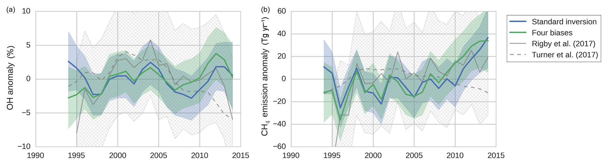
Figure 6The results of two inversions of the two-box model: tropospheric OH anomalies (a) and CH4 emission anomalies (b). In the standard inversion, we kept IH transport, NH ∕ SH OH ratio, and stratospheric loss of MCF constant, and we used NOAA observations. In the second inversion, we implemented all four bias corrections instead (as described in Sect. 2.8). Both the mean anomalies and the 1-standard-deviation envelopes are shown, where anomalies were taken relative to the time-averaged mean in each respective ensemble member. Plotted in grey are the anomalies as derived by Rigby et al. (2017) (from the NOAA dataset) and by Turner et al. (2017) (from a combined NOAA and AGAGE dataset), adjusted so that they, too, average to zero. The 1-standard-deviation envelope from the Rigby et al. (2017) estimate is hatched in grey.
In this section, we present a comparison between the results of the standard inversion and an inversion that incorporated the four bias corrections (referred to as “four biases”). The inversion set-ups are described in Sect. 2.8. The OH and CH4 emission anomalies of both inversions are presented in Fig. 6, along with uncertainty envelopes of 1 standard deviation. The envelopes are wide, and with respect to these envelopes there were no significant differences between our two inversions. Interestingly, differences between the two inversions were the smallest in the 1998–2007 period, during which MCF is thought to provide the strongest constraint on OH (Montzka et al., 2011). Note that the final analysis period started from 1994 (rather than from 1990), because we only had sufficient NOAA coverage of MCF available from 1994 onwards.
Shown in grey in Fig. 6 are the anomalies derived by Rigby et al. (2017) (from the NOAA dataset) and by Turner et al. (2017). The four inversions showed qualitatively similar time dependencies, and differences generally fell within 1 standard deviation and always within 2 standard deviations. Differences with Turner et al. (2017) are largest, most notably after 2010, which can be expected since they use a combined AGAGE + NOAA dataset, whereas we only use NOAA data. In Rigby et al. (2017) it was shown that the use of a different dataset can result in different OH anomalies, though these differences were insignificant with respect to their uncertainty envelopes. Also visible is the uncertainty envelope of 1 standard deviation from Rigby et al. (2017), which is notably larger than our envelopes. This is likely due to a combination of the higher observational uncertainties and the higher number of optimized parameters adopted in Rigby et al. (2017). Further discussion of differences with these two studies is provided in Sect. 4.
Table 3Five metrics that describe the outcome of the two-box inversions. The two-box inversions listed are the standard set-up, four inversions with one bias implemented, and one inversion with all biases implemented. From left to right: (1) mean absolute error (MAE) in OH anomalies between the standard inversion and each respective inversion, (2) trend in OH over the 1994–2015 period, (3) mean lifetime of MCF with respect to OH (tropospheric burden MCF divided by total loss to OH), (4) mean total tropospheric lifetime of CH4 (tropospheric burden CH4 divided by total loss CH4), and (5) mean annual CH4 emissions (with soil sink).
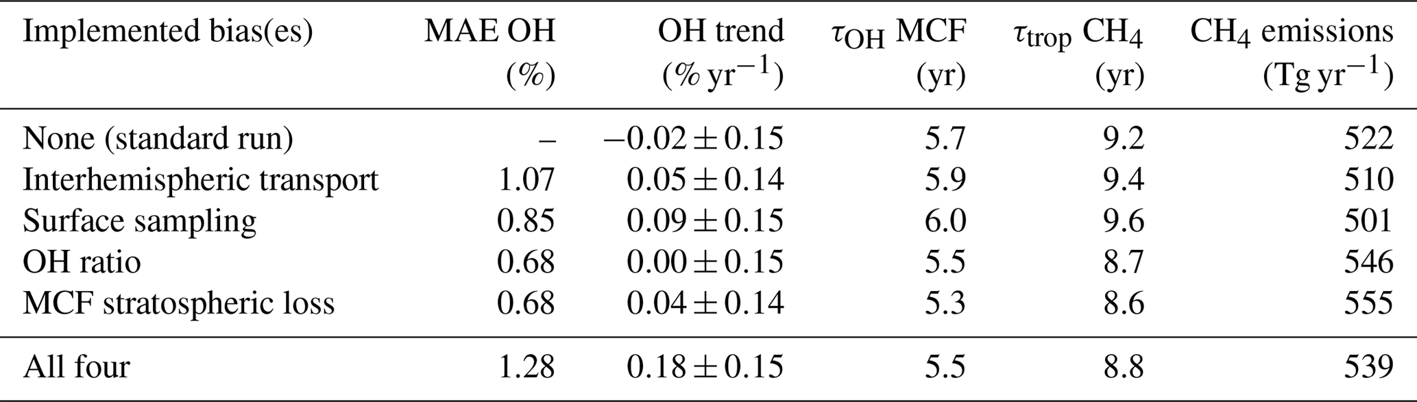
It is illustrative to further investigate how the identified biases impact the results. For this purpose, Table 3 presents five metrics for each of the two inversions as well as for inversions where we implemented the bias corrections one by one (taking standard settings for the other parameters).
The first metric is the mean absolute error (MAE) in the OH anomalies between each respective inversion and the standard inversion. The MAE provides an estimate of how much the OH estimate in a given year is affected by accounting for the bias. The highest MAE of 1.3 % is small compared to the full envelope of each individual OH inversion (3 %–4 %). This means that in terms of interannual variability over the entire period, the outcome was not affected by the biases much. However, as most biases showed their strongest trends over short periods, the peak values of the differences between inversions even out somewhat when averaging over the entire period.
Secondly, we derived an OH trend for each inversion set-up. As described in Sect. 2.1, we mapped the uncertainty of each inversion set-up in a Monte Carlo ensemble of inversions. We fitted a linear trend to the derived OH time series of each ensemble member. From the resulting collection of linear fit coefficients, we derived a mean linear fit coefficient and its standard deviation. Differences between the OH trends derived from the different inversions are insignificant. However, it is interesting to see that when all four biases are combined, we derived a shift to more positive OH trends. In the standard inversion, 43 % of the ensemble shows a positive trend, whereas in the four-bias inversion 88 % of the ensemble shows a positive trend.
The final three metrics are the tropospheric lifetime of MCF with respect to OH (, as in Eq. 1), the total tropospheric lifetime of CH4 (, as in Eq. 1), and the derived global mean CH4 emissions, averaged over the 1994–2015 period. For global CH4 emissions, we added the soil sink (32 [26–42] Tg yr−1; Kirschke et al., 2013), which was not included in the two-box model set-up. Naturally, these three are strongly correlated. When we compare the relative differences in, for example, the lifetime of MCF with respect to OH between different inversion set-ups to the MAE in anomalies, it is clear that the systematic offset between the different inversions (up to 10 %) was much higher than the differences in anomalies (up to 1.3 %). This is similar to what was seen for the biases themselves, where the systematic component tended to be much higher than the temporal variations (e.g. the bias in the IH OH ratio, shown in Fig. 4). We discuss this offset in more detail in Sect. 4.
A first point that deserves discussion is the low global CH4 emissions (1994–2015) we derived compared to those reported in literature. Our best estimate corresponds to 539 Tg yr−1 (Table 3), which is significantly lower than the 580–600 Tg yr−1 estimates reported by the two-box inversions of Turner et al. (2017) and Rigby et al. (2017). Our estimate is also on the low end of 3-D modelling studies; Saunois et al. (2016) derived CH4 emissions from 30 3-D model inversions and found emissions of 558 [540–570] Tg yr−1 over the 2000–2012 period. Bousquet et al. (2006) performed a full 3-D inversion of CH4, using OH fields that were optimized against MCF in a separate 3-D model inversion (Bousquet et al., 2005). In their study, CH4 emissions of 525±8 Tg yr−1 were found over the 1984–2003 period, so their estimate does not include the renewed CH4 growth.
We found that several factors contribute to the differences. Firstly, in the model used by Turner et al. (2017) the atmospheric mass was taken as the global atmospheric mass (5.15×10¹⁸ kg), whereas we used the tropospheric mass (4.4×10¹⁸ kg). When we ran our two-box inversion with the global atmospheric mass, we also found emissions close to 600 Tg yr−1. Secondly, we could close the gap with Rigby et al. (2017) by adjusting our a priori two-box model parameters. Specifically, when we adopted an IH exchange rate and an IH OH ratio similar to theirs (1.4 yr−1 and 1.07 respectively) in our standard inversion, we found global CH4 emissions of 595 Tg yr−1. This points to a strong sensitivity of the derived CH4 emissions to these parameters of the two-box model, which in our case are derived from full 3-D TM5 model simulations.
In our standard 3-D simulation, the IH gradient of MCF tended to be overestimated compared to observations from the NOAA network up to 2005, while global mean mixing ratios were captured much better. Translated into our two-box model, an inversion would tend to reduce MCF emissions to efficiently bring down the IH MCF gradient. To subsequently close the global MCF budget, OH will be reduced, resulting in lower global CH4 emissions in the two-box model inversion. The lower CH4 emissions we derived in our two-box model inversion are thus in line with the overestimated MCF latitudinal gradient in TM5. There are several possible explanations for this overestimate.
Firstly, MCF emissions that we used in our 3-D simulation were too high. In our two-box inversion, we found significantly lower MCF emissions (∼10 %–30 %) than the prior estimate based on emission inventories, with the exception of the 2010–2014 period. Liang et al. (2017) also derived MCF emissions from the IH gradient and found these to be systematically lower than those based on bottom-up industrial inventories. Secondly, the NH : SH OH ratio might be higher than 0.98 (Spivakovsky et al., 2000; Patra et al., 2011) and more in line with higher estimates from atmospheric chemistry simulations (Naik et al., 2013). Thirdly, a higher fraction of MCF emissions could be located in the SH (15 %–20 % instead of 5 %–10 %). Finally, IH exchange in TM5 could be too slow. A combination of the last two points would also arise if MCF emissions moved from NH mid-latitudes to NH low latitudes (e.g. India), since low-latitude emissions will be exchanged more rapidly with the SH. At this point it is not clear which of these explanations is most likely.
As is acknowledged in the previous two-box inversion studies of OH (Rigby et al., 2017; Turner et al., 2017), the problem of deriving OH from MCF and to a lesser degree from CH4 is strongly under-constrained. Therefore, many solutions fit the problem almost equally well. Moreover, a best estimate, or most likely solution, derived from a two-box model is a function of uncertain input parameters. For example, if it is assumed a priori that OH can only vary within a small band of 2 %, then a most likely solution with small OH variations will be found. In this study, we have identified a number of parameters which show variations outside of conventionally assumed bounds. As such, for these parameters, the variations we find are never fully explored in a conventional two-box model inversion, even if done as comprehensively as in Rigby et al. (2017). A clear example is stratospheric loss of MCF, which is generally assumed to have only small variability (10 % to 20 %). Here, we found a persistent 68 % drop in loss of MCF to the stratosphere. Potentially, this loss rate can recover if MCF emissions stop decreasing. Similarly, we find variations in transport of MCF of up to 20 % that persist for multiple years, compared to a conventional uncertainty in IH exchange of 10 %. In the 1994–1998 period, during a period of strong redistribution of MCF, the individual impact of each of the four biases was quite high, though when combined in one inversion the biases partly cancelled. During the 1998–2007 period, derived OH was less sensitive to the derived biases, likely due to a combination of a small role of uncertain emissions in the MCF budget (Montzka et al., 2011) and a period of relatively small redistribution of MCF. After this period, as MCF abundance continued to decline, we saw a growing impact from the IH exchange bias, as MCF emissions were increasingly constrained from the IH gradient, rather than from the emission inventory.
Another crucial parameter in the two-box inversion is the uncertainty in the global mean mixing ratios and in the IH gradient, as these uncertainties quantify the information content of the observational records. We provided an independent estimate of the uncertainty using 3-D model output in Sect. 3.1.2, summarized in Table 2. We can compare the uncertainties we find to observational uncertainties as derived from bootstrapping by Turner et al. (2017). They find uncertainties in hemispheric means of 6–8 ppb for CH4 and of 5 %–6 % for MCF. Clearly, this is much higher than what we find, and their uncertainties seem to be an overestimate considering the limited sensitivity of our result to a different source–sink distribution. In their most likely solution, derived OH variations were such that the observed post-2007 renewed growth of CH4 coincides with a decrease in CH4 emissions. This solution does not fall within the uncertainty envelope we derived here (right panel in Fig. 6). The difference in observational uncertainties is likely an important reason for this; their solution corresponds to a statistical inversion framework where less weight is given to the observations.
In the end, conclusions from our study and those drawn by Rigby et al. (2017) and Turner et al. (2017) remain qualitatively similar. The post-2007 renewed growth of CH4 need not be caused by a sudden increase in emissions in 2007. Rather, emissions could have increased more gradually over the 1994–2007 period, while CH4 growth was suppressed temporarily by elevated OH levels. The lack of sensitivity of the inversion to the bias corrections and the large remaining uncertainty envelope in the final inversion both indicate that there are other parameters that result in significant uncertainties. Examples are the emission fraction in the NH, observational uncertainties, and uncertainty in the emission timing of MCF. Thus, while a first step can be made through the incorporation of 3-D model information, we confirm the conclusion drawn in Rigby et al. (2017) and Turner et al. (2017) that the current state of the problem is still strongly underdetermined.
In another recent study, an effort was made to find tracer alternatives to MCF (Liang et al., 2017). For this, their suggested method was to use 3-D model output to improve the results of a two-box model through intelligent parametrizations. Clearly, this is similar to the work described here. For example, similar to us, they found different IH exchange timescales for different tracers. However, we explicitly resolved the two-box model in the 3-D framework, while their study focused mostly on fitting parameters empirically to find a match between two-box and 3-D model results. Additionally, for the parametrization, Liang et al. (2017) used hemispheric mean mixing ratios derived from the surface network, whereas we based mixing ratios on the full (hemispheric) troposphere in TM5. We identified a trend and strong, persistent variations in IH transport (CH4 and MCF) and in the surface sampling bias (MCF) which were not identified in Liang et al. (2017). Additionally, they described a two-box strategy in which two tracers are used to derive the IH OH ratio, which can then also be used for other tracers. Our work suggests that there should be careful consideration of different IH OH ratios seen by different tracers and potential trends therein. A two-box inversion is sensitive to the IH OH ratio, and we have shown that the effective IH OH ratio a tracer is exposed to depends strongly on that tracer's source–sink distribution. Some of the differences between their findings and ours may be explained by the definition of a hemispheric mean mixing ratio (surface-based versus full troposphere), but further reconciliation of the two approaches in future research is necessary.
It is worth noting that the TM5 model, on which the two-box parametrization is based, has its own limitations, and so has treating TM5 as “the truth”. For example, our simulations were done on the coarse horizontal resolution of . This would have impacted how well NOAA background sites were actually situated in the background. We checked that the TM5-derived observational time series were not systematically more polluted than the real-world NOAA-GMD observations. For this, we detrended and deseasonalized the CH4 and MCF time series per surface site and quantified the spread in the residuals. At most sites, we found no offset between residual spread in the TM5-derived versus the real-world time series. At a small number of sites, TM5-derived time series showed more spread in residuals, while at others the spread was less. Therefore, we found no evidence for systematic biases in TM5-sampled observations. Additionally, any transport model is susceptible to some form of transport errors, and using a different 3-D model for the two-box parametrization will likely result in different parameters. Therefore, we are careful in suggesting quantitative interpretation of our results. Certain aspects of the biases, such as a slowdown of MCF loss to the stratosphere and the strong variations in IH transport of MCF, are likely to also be found in other 3-D transport models, as they are a direct consequence of the MCF emissions drop. Other aspects, such as the exact interannual variations of IH transport of CH4 or the 7 % offset between the physical OH ratio and the effective OH ratio, should be interpreted with more care, as these more strongly depend on the input emission and loss fields and on the exact treatment of transport in the 3-D model. Additional sensitivity tests done in multiple transport models can help in identifying sensitivities of the derived bias corrections. However, our analysis does show a potential for these biases to arise, and TM5 is a good starting point for exploring them, as TM5 has provided a strong basis for a wide variety of studies in the past (e.g. Alexe et al., 2015; Laan-Luijkx et al., 2015; Bândă et al., 2016).
In this study, we investigated variations in the global atmospheric oxidizing capacity in conjunction with variations in the global CH4 budget. We specifically revisited the use of two-box models to infer information about these quantities using global observations of MCF and CH4.
We identified four two-box model parameters that can benefit from 3-D model-derived information. Two of these are known and obvious (IH transport and surface sampling bias), while the other two are less so (stratospheric loss and IH OH ratio). Two-box model parameters for these processes that were quantified from full 3-D model output showed strong temporal trends mainly for MCF, which have not been identified in any previous research. In general, the biases resulted from a combination of variations in transport and in the spatio-temporal source–sink distributions of each tracer.
We tested the impact of each of the biases in a two-box model inversion. As expected, we found that absolute OH and thus absolute CH4 emissions show large deviations between the different inversions (∼10 %). Given that large parts of these deviations were constant through time, they do not necessarily impact conclusions of past two-box modelling studies that focused on interannual variations.
Compared to the absolute differences, we found only small differences in OH anomalies (up to 1.3 %, averaged over 1994–2015) relative to the full uncertainty envelope found here (3 %–4 %) or in Rigby et al. (2017) (8 %). This indicates that significant uncertainties in parameters unrelated to the identified biases remain. As such, we confirm in large part the conclusions drawn by Rigby et al. (2017) and Turner et al. (2017) regarding the underdetermined state of the problem. In the end, we did find that the conclusions one can draw from each individual inversion could be strongly affected by the bias corrections; in the standard inversion only 43 % of our Monte Carlo ensemble showed a positive trend in OH over the 1994–2015 period, compared to 88 % in the four-bias inversion.
The identified two-box model biases contribute to the already significant uncertainty in derived OH, and properly accounting for them can be a piece in the puzzle of improving constraints on OH. Moving forward, a likely next step is to incorporate more tracers in an effort to further tighten constraints on OH. In such a scenario, the tracer-dependent nature of the biases will likely increase the bias impact, and a proper 3-D model analysis for each tracer becomes even more important. Already, efforts have been made to do so (Liang et al., 2017), and in this study we provide further suggestions for such an approach. A distinct advantage in this approach is that information from multiple 3-D transport models can be used to tune the two-box inversion, making the inversion outcome less reliant on transport parametrizations of any single 3-D transport model. Additionally, computational efficiency of simple models allows for complex statistical inversion frameworks, incorporating, for example, hierarchical uncertainties (Rigby et al., 2017).
On the other hand, the biases are often dependent on the sources and sinks used in the 3-D model simulation. As such, a feedback loop between the two-box inversion and the 3-D transport models might be necessary to correctly derive bias corrections, which makes such an analysis cumbersome. Additionally, a bias such as that in IH exchange of MCF might be difficult to resolve at all, because IH exchange of MCF is ill-defined in a two-box model (see Sects. 3.1.1 and S4). Therefore, we deem it important that a multi-tracer inversion in a full 3-D model should also be performed, similar to the 3-D inversion of MCF performed by Bousquet et al. (2005) but extended to more recent years. As an added advantage, a 3-D model inversion would increase the pool of potential tracers that can be implemented to constrain OH. For example, the short-lived tracer 14CO has been identified as a potential tracer to constrain OH (Brenninkmeijer et al., 1992; Quay et al., 2000; Krol et al., 2008) but would not be implementable in a two-box model.
For access to any of the data presented in this study, but not included in the supplements, please contact Stijn Naus (stijn.naus@wur.nl). All data are available on request.
The supplement related to this article is available online at: https://doi.org/10.5194/acp-19-407-2019-supplement.
MK, SN and SM designed the research. SN wrote the manuscript with major input from MK, and further contributions from all co-authors. SN performed the two-box simulations. SN and SP performed the TM5 simulations. MK supervised the research. All authors discussed the results and contributed to the final manuscript.
The authors declare that they have no conflict of interest.
This work was carried out on the Dutch National e-Infrastructure with the
support of SURF Cooperative. This work was funded through the Netherlands
Organisation for Scientific Research (NWO), project number
824.15.002.
Edited by: Rolf
Müller
Reviewed by: two anonymous referees
Alexe, M., Bergamaschi, P., Segers, A., Detmers, R., Butz, A., Hasekamp, O., Guerlet, S., Parker, R., Boesch, H., Frankenberg, C., Scheepmaker, R. A., Dlugokencky, E., Sweeney, C., Wofsy, S. C., and Kort, E. A.: Inverse modelling of CH4 emissions for 2010–2011 using different satellite retrieval products from GOSAT and SCIAMACHY, Atmos. Chem. Phys., 15, 113–133, https://doi.org/10.5194/acp-15-113-2015, 2015. a
Bândă, N., Krol, M., Noije, T., Weele, M., Williams, J. E., Sager, P. L., Niemeier, U., Thomason, L., and Röckmann, T.: The effect of stratospheric sulfur from Mount Pinatubo on tropospheric oxidizing capacity and methane, J. Geophys. Res.-Atmos., 120, 1202–1220, 2015. a
Bândă, N., Krol, M., van Weele, M., van Noije, T., Le Sager, P., and Röckmann, T.: Can we explain the observed methane variability after the Mount Pinatubo eruption?, Atmos. Chem. Phys., 16, 195–214, https://doi.org/10.5194/acp-16-195-2016, 2016. a
Bousquet, P., Hauglustaine, D. A., Peylin, P., Carouge, C., and Ciais, P.: Two decades of OH variability as inferred by an inversion of atmospheric transport and chemistry of methyl chloroform, Atmos. Chem. Phys., 5, 2635–2656, https://doi.org/10.5194/acp-5-2635-2005, 2005. a, b, c, d, e, f
Bousquet, P., Ciais, P., Miller, J., Dlugokencky, E., Hauglustaine, D., Prigent, C., Van der Werf, G., Peylin, P., Brunke, E.-G., Carouge, C., Langenfelds, R. L., Lathière, J., Papa, F., Ramonet, M., Schmidt, M., Steele, L. P., Tyler, S. C., and White, J.: Contribution of anthropogenic and natural sources to atmospheric methane variability, Nature, 443, 439–443, 2006. a
Brenninkmeijer, C. A., Manning, M. R., Lowe, D. C., Wallace, G., Sparks, R. J., and Volz-Thomas, A.: Interhemispheric asymmetry in OH abundance inferred from measurements of atmospheric 14CO, Nature, 356, 50–52, 1992. a, b
Brühl, C. and Crutzen, P. J.: MPIC two-dimensional model, NASA Ref. Publ, Washington D.C., 1292, 103–104, 1993. a
Butchart, N.: The Brewer-Dobson circulation, Rev. Geophys., 52, 157–184, 2014. a
Chipperfield, M. P., Liang, Q., Abraham, L., Bekki, S., Braesicke, P., Dhomse, S., Di Genova, G., Fleming E. L., Hardiman, S., Iachetti, D., Jackman, C. H., Kinnison, D. E., Marchand, M., Pitari, G., Rozanov, E., Stenke, A., and Tummon, F. (authors); Burgalat, J., Cugnet, D., Frith, S. M., Pascoe, C., and Rigby, M. (contributors): Model estimates of lifetimes, in: SPARC, 2013: SPARC Report on the Lifetimes of Stratospheric Ozone-Deleting Substances, Their Replacements, and Related Species, edited by: Reimann, S., Ko, M. K. W., Newman, P. A., and Strahan, S. E., chap. 5, WCRP-15/2013, 2013. a, b, c
Dee, D. P., Uppala, S. M., Simmons, A. J., Berrisford, P., Poli, P., Kobayashi, S., Andrae, U., Balmaseda, M. A., Balsamo, G., Bauer, P., Beljaars, A. C. M., van de Berg, L., Bidlot, J., Bormann, N., Delsol, C., Dragani, R., Fuentes, M., Geer, A. J., Haimberger, L., Healy, S. B., Hersbach, H., Hólm, E. V., Isaksen, L., Kållberg, P., Köhler, M., Matricardi, M., McNally, A. P., Monge-Sanz, B. M., Morcrette, J.-J., Park, B.-K., Peubey, C., de Rosnay, P., Tavolato, C., Thépaut, J.-N., and Vitart, F.: The ERA-Interim reanalysis: Configuration and performance of the data assimilation system, Q. J. Roy. Meteor. Soc., 137, 553–597, 2011. a
Dlugokencky, E. J., Steele, L. P., Lang, P. M., and Masarie, K. A.: The growth rate and distribution of atmospheric methane, J. Geophys. Res.-Atmos., 99, 17021–17043, 1994. a, b
Dlugokencky, E. J., Bruhwiler, L., White, J. W. C., Emmons, L. K., Novelli, P. C., Montzka, S. A., Masarie, K. A., Lang, P. M., Crotwell, A. M., Miller, J. B., and Gatti, L. V.: Observational constraints on recent increases in the atmospheric CH4 burden, Geophys. Res. Lett., 36, https://doi.org/10.1029/2009GL039780, 2009. a
Fisher, M.: Estimating the covariance matrices of analysis and forecast error in variational data assimilation, ECMWF Tech. Mem., 220, https://doi.org/10.21957/1dxrasjit, 1995. a
Francey, R. J. and Frederiksen, J. S.: The 2009–2010 step in atmospheric CO2 interhemispheric difference, Biogeosciences, 13, 873–885, https://doi.org/10.5194/bg-13-873-2016, 2016. a
Huijnen, V., Williams, J., van Weele, M., van Noije, T., Krol, M., Dentener, F., Segers, A., Houweling, S., Peters, W., de Laat, J., Boersma, F., Bergamaschi, P., van Velthoven, P., Le Sager, P., Eskes, H., Alkemade, F., Scheele, R., Nédélec, P., and Pätz, H.-W.: The global chemistry transport model TM5: description and evaluation of the tropospheric chemistry version 3.0, Geosci. Model Dev., 3, 445–473, https://doi.org/10.5194/gmd-3-445-2010, 2010. a
Kirschke, S., Bousquet, P., Ciais, P., Saunois, M., Canadell, J. G., Dlugokencky, E. J., Bergamaschi, P., Bergmann, D., Blake, D. R., Bruhwiler, L., et al.: Three decades of global methane sources and sinks, Nat. Geosci., 6, 813–823, 2013. a
Krol, M., Houweling, S., Bregman, B., van den Broek, M., Segers, A., van Velthoven, P., Peters, W., Dentener, F., and Bergamaschi, P.: The two-way nested global chemistry-transport zoom model TM5: algorithm and applications, Atmos. Chem. Phys., 5, 417–432, https://doi.org/10.5194/acp-5-417-2005, 2005. a
Krol, M., de Bruine, M., Killaars, L., Ouwersloot, H., Pozzer, A., Yin, Y., Chevallier, F., Bousquet, P., Patra, P., Belikov, D., Maksyutov, S., Dhomse, S., Feng, W., and Chipperfield, M. P.: Age of air as a diagnostic for transport timescales in global models, Geosci. Model Dev., 11, 3109–3130, https://doi.org/10.5194/gmd-11-3109-2018, 2018. a
Krol, M. C. and Lelieveld, J.: Can the variability in tropospheric OH be deduced from measurements of 1,1,1-trichloroethane (methyl chloroform)?, J. Geophys. Res.-Atmos., 108, https://doi.org/10.1029/2002JD002423, 2003. a, b, c, d
Krol, M. C., Lelieveld, J., Oram, D. E., Sturrock, G. A., Penkett, S. A., Brenninkmeijer, C. A. M., Gros, V., Williams, J., and Scheeren, H. A.: Continuing emissions of methyl chloroform from Europe, Nature, 421, 131–135, 2003. a, b
Krol, M. C., Meirink, J. F., Bergamaschi, P., Mak, J. E., Lowe, D., Jöckel, P., Houweling, S., and Röckmann, T.: What can 14CO measurements tell us about OH?, Atmos. Chem. Phys., 8, 5033–5044, https://doi.org/10.5194/acp-8-5033-2008, 2008. a
Laan-Luijkx, I. T., Velde, I. R., Krol, M. C., Gatti, L. V., Domingues, L. G., Correia, C. S. C., Miller, J. B., Gloor, M., Leeuwen, T. T., Kaiser, J. W., Wiedinmyer, C., Basu, S., Clerbaux, C., and Peters, W.: Response of the Amazon carbon balance to the 2010 drought derived with CarbonTracker South America, Global Biogeochem. Cy., 29, 1092–1108, 2015. a
Lawrence, M. G., Jöckel, P., and von Kuhlmann, R.: What does the global mean OH concentration tell us?, Atmos. Chem. Phys., 1, 37–49, https://doi.org/10.5194/acp-1-37-2001, 2001. a, b
Liang, Q., Chipperfield, M. P., Fleming, E. L., Abraham, N. L., Braesicke, P., Burkholder, J. B., Daniel, J. S., Dhomse, S., Fraser, P. J., Hardiman, S. C., Jackman, C. H., Kinnison, D. E., Krummel, P. B., Montzka, S. A., Morgenstern, O., McCulloch, A., Mühle, J., Newman, P. A., Orkin, V. L., Pitari, G., Prinn, R. G., Rigby, M., Rozanov, E., Stenke, A., Tummon, F., Velders, G. J. M., Visioni, D., and Weiss, R. F.: Deriving Global OH Abundance and Atmospheric Lifetimes for Long-Lived Gases: A Search for CH3CCl3 Alternatives, J. Geophys. Res.-Atmos., 122, https://doi.org/10.1002/2017JD026926, 2017. a, b, c, d, e, f, g, h, i, j, k
Lovelock, J. E.: Methyl chloroform in the troposphere as an indicator of OH radical abundance, Nature, 267, 32–32, 1977. a
McCulloch, A. and Midgley, P. M.: The history of methyl chloroform emissions: 1951–2000, Atmos. Environ., 35, 5311–5319, 2001. a, b, c, d
McNorton, J., Chipperfield, M. P., Gloor, M., Wilson, C., Feng, W., Hayman, G. D., Rigby, M., Krummel, P. B., O'Doherty, S., Prinn, R. G., Weiss, R. F., Young, D., Dlugokencky, E., and Montzka, S. A.: Role of OH variability in the stalling of the global atmospheric CH4 growth rate from 1999 to 2006, Atmos. Chem. Phys., 16, 7943–7956, https://doi.org/10.5194/acp-16-7943-2016, 2016. a
Meirink, J. F., Bergamaschi, P., and Krol, M. C.: Four-dimensional variational data assimilation for inverse modelling of atmospheric methane emissions: method and comparison with synthesis inversion, Atmos. Chem. Phys., 8, 6341–6353, https://doi.org/10.5194/acp-8-6341-2008, 2008. a
Millet, D. B. and Goldstein, A. H.: Evidence of continuing methylchloroform emissions from the United States, Geophys. Res. Lett., 31, 4026, https://doi.org/10.1029/2004GL020166, 2004. a
Montzka, S. A., Spivakovsky, C. M., Butler, J. H., Elkins, J. W., Lock, L. T., and Mondeel, D. J.: New observational constraints for atmospheric hydroxyl on global and hemispheric scales, Science, 288, 500–503, 2000. a, b, c, d, e, f
Montzka, S. A., Krol, M., Dlugokencky, E. J., Hall, B., Jöckel, P., and Lelieveld, J.: Small interannual variability of global atmospheric hydroxyl, Science, 331, 67–69, 2011. a, b, c, d, e, f, g, h, i, j, k
Montzka, S. A., Dutton, G. S., Yu, P., Ray, E., Portmann, R. W., Daniel, J. S., Kuijpers, L., Hall, B. D., Mondeel, D., Siso, C., Nance, J. D., Rigby, M., Manning, A. J., Hu, L., Moore, F., Miller, B. R., and Elkins, J. W: An unexpected and persistent increase in global emissions of ozone-depleting CFC-11, Nature, 557, 413–417, https://doi.org/10.1038/s41586-018-0106-2, 2018. a
Naik, V., Jain, A. K., Patten, K. O., and Wuebbles, D. J.: Consistent sets of atmospheric lifetimes and radiative forcings on climate for CFC replacements: HCFCs and HFCs, J. Geophys. Res.-Atmos., 105, 6903–6914, 2000. a, b
Naik, V., Voulgarakis, A., Fiore, A. M., Horowitz, L. W., Lamarque, J.-F., Lin, M., Prather, M. J., Young, P. J., Bergmann, D., Cameron-Smith, P. J., Cionni, I., Collins, W. J., Dalsøren, S. B., Doherty, R., Eyring, V., Faluvegi, G., Folberth, G. A., Josse, B., Lee, Y. H., MacKenzie, I. A., Nagashima, T., van Noije, T. P. C., Plummer, D. A., Righi, M., Rumbold, S. T., Skeie, R., Shindell, D. T., Stevenson, D. S., Strode, S., Sudo, K., Szopa, S., and Zeng, G.: Preindustrial to present-day changes in tropospheric hydroxyl radical and methane lifetime from the Atmospheric Chemistry and Climate Model Intercomparison Project (ACCMIP), Atmos. Chem. Phys., 13, 5277–5298, https://doi.org/10.5194/acp-13-5277-2013, 2013. a, b
Pandey, S., Houweling, S., Krol, M., Aben, I., Chevallier, F., Dlugokencky, E. J., Gatti, L. V., Gloor, E., Miller, J. B., Detmers, R., Machida, T., and Röckmann, T.: Inverse modeling of GOSAT-retrieved ratios of total column CH4 and CO2 for 2009 and 2010, Atmos. Chem. Phys., 16, 5043–5062, https://doi.org/10.5194/acp-16-5043-2016, 2016. a
Pandey, S., Houweling, S., Krol, M., Aben, I., Monteil, G., Nechita-Banda, N., Dlugokencky, E. J., Detmers, R., Hasekamp, O., Xu, X., Riley, W. J., Poulter, B., Zhang, Z., McDonald, K. C., White, J. W. C., Bousquet, P., and Röckmann, T.: Enhanced methane emissions from tropical wetlands during the 2011 La Niña, Sci. Rep., 7, 45759, https://doi.org/10.1038/srep45759, 2017. a
Patra, P. K., Houweling, S., Krol, M., Bousquet, P., Belikov, D., Bergmann, D., Bian, H., Cameron-Smith, P., Chipperfield, M. P., Corbin, K., Fortems-Cheiney, A., Fraser, A., Gloor, E., Hess, P., Ito, A., Kawa, S. R., Law, R. M., Loh, Z., Maksyutov, S., Meng, L., Palmer, P. I., Prinn, R. G., Rigby, M., Saito, R., and Wilson, C.: TransCom model simulations of CH4 and related species: linking transport, surface flux and chemical loss with CH4 variability in the troposphere and lower stratosphere, Atmos. Chem. Phys., 11, 12813–12837, https://doi.org/10.5194/acp-11-12813-2011, 2011. a, b, c, d
Patra, P. K., Krol, M. C., Montzka, S. A., Arnold, T., Atlas, E. L., Lintner, B. R., Stephens, B. B., Xiang, B., Elkins, J. W., Fraser, P. J., Ghosh, A., Hintsa, E. J., Hurst, D. F., Ishijima, K., Krummel, P. B., Miller, B. R., Miyazaki, K., Moore, F. L., Mühle, J., O'Doherty, S., Prinn, R. G., Steele, L. P., Takigawa, M., Wang, H. J., Weiss, R. F., Wofsy, S. C., and Young, D.: Observational evidence for interhemispheric hydroxyl-radical parity, Nature, 513, 219–223, 2014. a, b
Prinn, R., Cunnold, D., Rasmussen, R., Simmonds, P., Alyea, F., Crawford, A., Fraser, P., and Rosen, R.: Atmospheric trends in methylchloroform and the global average for the hydroxyl radical, Science, 238, 945–950, 1987. a
Prinn, R., Cunnold, D., Simmonds, P., Alyea, F., Boldi, R., Crawford, A., Fraser, P., Gutzler, D., Hartley, D., Rosen, R., and Rasmussen, R.: Global average concentration and trend for hydroxyl radicals deduced from ALE/GAGE trichloroethane (methyl chloroform) data for 1978–1990, J. Geophys. Res.-Atmos., 97, 2445–2461, 1992. a
Prinn, R. G., Huang, J., Weiss, R. F., Cunnold, D. M., Fraser, P. J., Simmonds, P. G., McCulloch, A., Harth, C., Reimann, S., Salameh, P., O'Doherty, S., Wang, R. H. J., Porter, L. W., Miller, B. R., and Krummel, P. B.: Evidence for variability of atmospheric hydroxyl radicals over the past quarter century, Geophys. Res. Lett., 32, L07809, https://doi.org/10.1029/2004GL022228, 2005. a, b
Prinn, R. G., Weiss, R. F., Arduini, J., Arnold, T., DeWitt, H. L., Fraser, P. J., Ganesan, A. L., Gasore, J., Harth, C. M., Hermansen, O., Kim, J., Krummel, P. B., Li, S., Loh, Z. M., Lunder, C. R., Maione, M., Manning, A. J., Miller, B. R., Mitrevski, B., Mühle, J., O'Doherty, S., Park, S., Reimann, S., Rigby, M., Saito, T., Salameh, P. K., Schmidt, R., Simmonds, P. G., Steele, L. P., Vollmer, M. K., Wang, R. H., Yao, B., Yokouchi, Y., Young, D., and Zhou, L.: History of chemically and radiatively important atmospheric gases from the Advanced Global Atmospheric Gases Experiment (AGAGE), Earth Syst. Sci. Data, 10, 985–1018, https://doi.org/10.5194/essd-10-985-2018, 2018. a
Quay, P., Stutsman, J., Wilbur, D., Snover, A., Dlugokencky, E. J., and Brown, T.: The isotopic composition of atmospheric methane, Global Biogeochm. Cy., 13, 445–461, 1999. a
Quay, P., King, S., White, D., Brockington, M., Plotkin, B., Gammon, R., Gerst, S., and Stutsman, J.: Atmospheric 14CO: A tracer of OH concentration and mixing rates, J. Geophys. Res.-Atmos., 105, 15147–15166, 2000. a
Reimann, S., Manning, A. J., Simmonds, P. G., Cunnold, D. M., Wang, R. H. J., Li, J., McCulloch, A., Prinn, R. G., Huang, J., Weiss, R. F., Fraser, P. J., O'Doherty, S., Greally, B. R., Stemmler, K., Hill, M., and Folini, D.: Low European methyl chloroform emissions inferred from long-term atmospheric measurements, Nature, 433, 506–508, 2005. a
Rigby, M., Prinn, R. G., O'Doherty, S., Montzka, S. A., McCulloch, A., Harth, C. M., Mühle, J., Salameh, P. K., Weiss, R. F., Young, D., Simmonds, P. G., Hall, B. D., Dutton, G. S., Nance, D., Mondeel, D. J., Elkins, J. W., Krummel, P. B., Steele, L. P., and Fraser, P. J.: Re-evaluation of the lifetimes of the major CFCs and CH3CCl3 using atmospheric trends, Atmos. Chem. Phys., 13, 2691–2702, https://doi.org/10.5194/acp-13-2691-2013, 2013. a
Rigby, M., Montzka, S. A., Prinn, R. G., White, J. W. C., Young, D., O'Doherty, S., Lunt, M. F., Ganesan, A. L., Manning, A. J., Simmonds, P. G., Salameh, P. K., Harth, C. M., Mühle, J., Weiss, R. F., Fraser, P. J., Steele, L. P., Krummel, P. B., McCulloch, A., and Park, S.: Role of atmospheric oxidation in recent methane growth, P. Natl. Acad. Sci. USA, 114, 5373–5377, 2017. a, b, c, d, e, f, g, h, i, j, k, l, m, n, o, p, q, r, s, t, u, v, w, x, y, z, aa, ab, ac, ad
Saunois, M., Bousquet, P., Poulter, B., Peregon, A., Ciais, P., Canadell, J. G., Dlugokencky, E. J., Etiope, G., Bastviken, D., Houweling, S., Janssens-Maenhout, G., Tubiello, F. N., Castaldi, S., Jackson, R. B., Alexe, M., Arora, V. K., Beerling, D. J., Bergamaschi, P., Blake, D. R., Brailsford, G., Brovkin, V., Bruhwiler, L., Crevoisier, C., Crill, P., Covey, K., Curry, C., Frankenberg, C., Gedney, N., Höglund-Isaksson, L., Ishizawa, M., Ito, A., Joos, F., Kim, H.-S., Kleinen, T., Krummel, P., Lamarque, J.-F., Langenfelds, R., Locatelli, R., Machida, T., Maksyutov, S., McDonald, K. C., Marshall, J., Melton, J. R., Morino, I., Naik, V., O'Doherty, S., Parmentier, F.-J. W., Patra, P. K., Peng, C., Peng, S., Peters, G. P., Pison, I., Prigent, C., Prinn, R., Ramonet, M., Riley, W. J., Saito, M., Santini, M., Schroeder, R., Simpson, I. J., Spahni, R., Steele, P., Takizawa, A., Thornton, B. F., Tian, H., Tohjima, Y., Viovy, N., Voulgarakis, A., van Weele, M., van der Werf, G. R., Weiss, R., Wiedinmyer, C., Wilton, D. J., Wiltshire, A., Worthy, D., Wunch, D., Xu, X., Yoshida, Y., Zhang, B., Zhang, Z., and Zhu, Q.: The global methane budget 2000–2012, Earth Syst. Sci. Data, 8, 697–751, https://doi.org/10.5194/essd-8-697-2016, 2016. a
Schaefer, H., Fletcher, S. E. M., Veidt, C., Lassey, K. R., Brailsford, G. W., Bromley, T. M., Dlugokencky, E. J., Michel, S. E., Miller, J. B., Levin, I., Lowe, D. C., Martin, R. J., Vaughn, B. H., and White, J. W. C.: A 21st-century shift from fossil-fuel to biogenic methane emissions indicated by 13CH4, Science, 352, 80–84, 2016. a
Schwietzke, S., Sherwood, O. A., Bruhwiler, L. M. P., Miller, J. B., Etiope, G., Dlugokencky, E. J., Michel, S. E., Arling, V. A., Vaughn, B. H., White, J. W. C., and Tans, P. P. : Upward revision of global fossil fuel methane emissions based on isotope database, Nature, 538, 88–91, 2016. a
Spivakovsky, C. M., Logan, J. A., Montzka, S. A., Balkanski, Y. J., Foreman-Fowler, M., Jones, D. B. A., Horowitz, L. W., Fusco, A. C., Brenninkmeijer, C. A. M., Prather, M. J., Wofsy, S. C., and McElroy, M. B.: Three-dimensional climatological distribution of tropospheric OH: Update and evaluation, J. Geophys. Res.-Atmos., 105, 8931–8980, 2000. a, b, c, d
Tsuruta, A., Aalto, T., Backman, L., Hakkarainen, J., van der Laan-Luijkx, I. T., Krol, M. C., Spahni, R., Houweling, S., Laine, M., Dlugokencky, E., Gomez-Pelaez, A. J., van der Schoot, M., Langenfelds, R., Ellul, R., Arduini, J., Apadula, F., Gerbig, C., Feist, D. G., Kivi, R., Yoshida, Y., and Peters, W.: Global methane emission estimates for 2000-2012 from CarbonTracker Europe-CH4 v1.0, Geosci. Model Dev., 10, 1261-1289, https://doi.org/10.5194/gmd-10-1261-2017, 2017. a
Turner, A. J., Frankenberg, C., Wennberg, P. O., and Jacob, D. J.: Ambiguity in the causes for decadal trends in atmospheric methane and hydroxyl, P. Natl. Acad. Sci. USA., 114, 5367–5372, https://doi.org/10.1073/pnas.1616020114, 2017. a, b, c, d, e, f, g, h, i, j, k, l, m, n, o, p, q, r, s, t, u
Walker, S. J., Weiss, R. F., and Salameh, P. K.: Reconstructed histories of the annual mean atmospheric mole fractions for the halocarbons CFC-11 CFC-12, CFC-113, and carbon tetrachloride, J. Geophys. Res.-Oceans, 105, 14285–14296, 2000. a
Wennberg, P. O., Peacock, S., Randerson, J. T., and Bleck, R.: Recent changes in the air-sea gas exchange of methyl chloroform, Geophys. Res. Lett., 31, 112, https://doi.org/10.1029/2004GL020476, 2004. a