the Creative Commons Attribution 4.0 License.
the Creative Commons Attribution 4.0 License.
 | 29 Mar 2019
Rethinking Craig and Gordon's approach to modeling isotopic compositions of marine boundary layer vapor
Eric S. Posmentier
Leslie J. Sonder
Naixin Fan
We develop a one-dimensional (1-D) steady-state isotope marine boundary layer (MBL) model that includes meteorologically important features missing in models of the Craig and Gordon type, namely height-dependent diffusion and mixing, lifting to deliver air to the free troposphere, and convergence of subsiding air. Kinetic isotopic fractionation results from this height-dependent diffusion that starts as pure molecular diffusion at the air–water interface and increases with height due to turbulent eddies. Convergence causes mixing of dry, isotopically depleted air with ambient air. Model results fill a quadrilateral in δD–δ18O space, of which three boundaries are defined by (1) vapor in equilibrium with various sea surface temperatures (SSTs), (2) mixing of vapor in equilibrium with seawater and vapor in subsiding air, and (3) vapor that has experienced maximum possible kinetic fractionation. Model processes also cause variations in d-excess of MBL vapor. In particular, mixing of relatively high d-excess descending and converging air into the MBL increases d-excess, even without kinetic isotope fractionation. The model is tested by comparison with seven data sets of marine vapor isotopic ratios, with excellent correspondence. About 95 % of observational data fall within the quadrilateral predicted by the model. The distribution of observations also highlights the significant influence of vapor from nearby converging descending air on isotopic variations within the MBL. At least three factors may explain the ∼5 % of observations that fall slightly outside of the predicted regions in δD–δ18O and d-excess–δ18O space: (1) variations in seawater isotopic ratios, (2) variations in isotopic composition of subsiding air, and (3) influence of sea spray.
- Article
(4463 KB) - Full-text XML
-
Supplement
(212 KB) - BibTeX
- EndNote


Stable isotopic ratios of water have been widely used to study the hydrologic cycle of the atmosphere. They have proven to be a powerful tool for understanding modern atmospheric processes (e.g., Dansgaard, 1964; Lawrence et al., 2004; Worden et al., 2007; Uemura et al., 2008; Kurita, 2011; Kopec et al., 2016). In addition, they have been extremely useful for inferring paleoclimate conditions and making climate reconstructions from glacier ice, tree rings, lake sediments, speleothems, and paleosols (e.g., Dansgaard et al., 1989; Wang et al., 2001; Huang et al., 2002; Andersen et al., 2004; Jouzel et al., 2007; Feng et al., 2007; Sheldon and Tabor, 2009; Masson-Delmotte et al., 2005a, b).
Sound interpretation of isotopic data requires a thorough understanding of all processes in the hydrological cycle that affect isotopic variations. These include (1) surface evaporation and processes in the planetary boundary layer (PBL) through which vapor reaches the overlying free atmosphere; (2) rainout and other processes along the trajectory of air masses transported to a precipitation site; (3) nucleation, growth, coalescence, and reevaporation of hydrometeors between the moisture source area and the precipitation site; and (4) subsequent processes affecting precipitation as it falls through the air. This study focuses on the first of these – surface evaporation and isotopologue concentrations within and fluxes through the PBL – in particular, the marine boundary layer (MBL), where ascending air delivers water vapor to the free atmosphere.
The PBL and the MBL have a variety of qualitative and quantitative definitions, not all consistent. In this discussion, we use the phrase “boundary layer” to refer to the lower part of the planetary or marine atmosphere, in which the flux of water vapor is close to vertical and vapor transport is accomplished primarily by turbulent or convective mixing. The troposphere above the MBL is often referred to as the “free atmosphere” or “free troposphere”, in which vapor transport is dominated by near-horizontal advection by winds. The thickness of the MBL varies from ∼100 to ∼1000 m or more with location, season, and time of day, as well as weather conditions (e.g., Christakos et al., 2013; Winning et al., 2017). In the MBL, unlike the terrestrial part of the PBL, water vapor is not affected by plant transpiration or variable surface wetness.
Craig and Gordon (1965) developed the first isotopic evaporation model, referred to hereafter as the C–G model, to calculate isotopic ratios of the evaporation vapor flux from the water surface when the humidity and isotopic composition in the “free air” are specified. The C–G model is based on the diffusive flux of an isotopologue (e.g., or HDO) through the boundary layer of the atmosphere. The diffusive flux is proportional to the difference in isotopic composition of vapor at the layer's boundaries and inversely proportional to the resistance of the layer to transport (Fick's law, described as a simple analogy of Ohm's law by C–G). The C–G model is conceptually a multiple “slab” (zero-dimensional) model. The slabs (layers), stacked from the bottom up, are turbulent ocean water, a laminar layer of ocean water that is affected by evaporation, the water–air interface, a laminar layer of air, a turbulent air layer, and the free atmosphere (where humidity and isotopic ratios no longer change rapidly with height). Even though each layer has a different resistance to vapor transport, the fundamental premise is that the vapor flux through all layers is the same. This premise follows in turn from the assumptions of quasi steady-state conditions, conservation of mass, and zero horizontal fluxes. Therefore, the flux entering the free atmosphere (at the top of the PBL) equals the evaporative flux at the water surface. The C–G model was tested and empirically parameterized using measurements of the isotopic evolution of an isolated body of evaporating water (Craig et al., 1963) and was subsequently successfully applied and adapted to many specific applications, including lake evaporation, leaf transpiration, and marine boundary layer processes. Interested readers can refer to Horita et al. (2008) for a comprehensive review of the status of the C–G model.
Particularly relevant to this study is the adaptation of the C–G model for the marine boundary layer. An influential study by Merlivat and Jouzel (1979) linked the magnitude of kinetic isotopic fractionation primarily within the laminar layer above the water–air interface, which is required input for the C–G model, to aerodynamic conditions, i.e., wind speed and surface ocean roughness. However, the model still required the input of the free atmosphere humidity and isotopic ratios. Recognizing the difficulty of knowing these free atmosphere variables, Merlivat and Jouzel (1979) made an assumption, known later as the “closure assumption”, that the isotopic ratios of vapor mass in the free atmosphere were equal to the isotopic ratios of the vapor fluxes from the sea surface. This assumption enabled them to complete a new multi-slab model (the M–J model), used by numerous investigators to calculate isotopic fluxes from the sea surface over a range of maritime conditions and to explore relationships between isotopic compositions of evaporative flux and boundary layer meteorological conditions such as sea surface temperature and relative humidity (e.g., Johnsen et al., 1989; Petit et al., 1991). The closure assumption also allowed the modeled flux to be used as the starting isotopic composition of an air mass, which evolves during subsequent transport and rainout or a Rayleigh process (e.g., Johnsen et al., 1989; Petit et al., 1991). The closure assumption, however, has been determined to be generally invalid at local scales (Jouzel and Koster, 1996). Nevertheless, it has continued to be used (e.g., Benetti et al., 2014) simply for lack of a better assumption.
Abandoning this closure assumption requires a fundamental rethinking of the MBL model structure. In addition, there are ramifications of other model assumptions. As a consequence, we consider three requirements for developing a useful, physically consistent MBL model free of the invalid closure assumption, a model with the purpose of determining the isotopic ratios of air ascending from the top of the MBL and entering the free atmosphere above.
First, vertical advection is necessary at the inception of a Rayleigh process in order to lift MBL air into the free atmosphere. When an air mass is lifted into the free troposphere, the vapor isotopic ratio of the air that first condenses during the Rayleigh process is equal to the isotopic ratio of vapor within the air mass, not the ratio of isotopologue diffusive fluxes into the air mass. Contrary to the closure assumption, these two are not generally equal (Jouzel and Koster, 1996). Therefore, an MBL model should calculate not only the isotopic ratio of vapor flux at the sea surface, but also that of vapor concentration within the MBL, particularly at the top of the MBL, and the latter is the quantity that should be used for the initial vapor isotopic composition in any subsequent Rayleigh process.
Second, with incorporation of vertical advection, mass balance requires (1) horizontal convergence of air within the MBL to replenish the lifted air in the evaporation column and (2) subsidence of air outside the model region to sustain the local horizontal convergence. Such a circulation on various scales was discussed by Craig and Gordon (1965) to explain why vapor in the MBL was not in isotopic equilibrium with ocean water. In this contribution, we attempt to quantify how horizontal convergence of air from non-local regions of subsidence affects the isotopic properties of the local MBL. Because the converging air is unlikely to have the same isotopic composition as the local MBL air, convergence turns out to affect MBL vapor isotopes quite significantly, as discussed later in this paper.
Third, incorporating convergence means that the assumption of constant vertical flux in the C–G model is no longer valid, even under steady-state conditions. This necessitates different equations of mass conservation.
These three model requirements obviously necessitate rethinking the C–G approach to constructing a model and they draw a sharp divergence between our model and the model of C–G and its extensions (e.g., Merlivat and Jouzel, 1979; Benetti et al., 2015). In addressing these three required changes, we find it advantageous to incorporate two additional changes to the model structure. The fourth major change is to abandon previous multi-slab models (referred to hereafter as C–G-type models) and to adopt instead a true one-dimensional (1-D) model in which quantities such as flux change continuously with height. In doing so, we describe a coefficient of turbulent transport that increases with height (see below). This yields the additional benefit of the ability to obtain isotopic ratios of air and vapor flux at any given height within the MBL.
The fifth major change is to abandon the need to specify the kinetic fractionation factor required by C–G-type models. In the boundary layer, the eddy diffusion coefficient (coefficient of turbulent transport by eddies) increases continuously with height (Merlivat and Coantic, 1975) from zero at the air–water interface, where transport of vapor is affected solely by isotopically fractionating molecular diffusion, to greater values at heights where vapor transport is dominated by turbulent eddies. Such a height-dependent change in diffusion coefficient is adopted in our model. As a result, our model is relieved of the need (1) to empirically choose the value of a parameterized kinetic fractionation factor (Δε in Craig and Gordon, 1965; k in Merlivat and Jouzel, 1979; this choice may sometimes be difficult and values reported in the literature may not apply to the specific conditions under investigation; e.g., Xiao et al., 2017) and (2) to assume a specific laminar layer thickness. Instead, we allow the total diffusion coefficient to represent pure molecular diffusion at the interface (which differs for different isotopologues and thus leads to kinetic fractionation) and to increase linearly with height to several orders of magnitude greater than molecular diffusivities. As a result, the laminar layer thickness scale becomes a diagnostic variable. The fourth and fifth major changes further sharpen the distinction between our model and C–G-type models.
Abandoning some of the assumptions of earlier models, such as constant flux of vapor isotopologues, flux equal to concentration (the invalid closure assumption), and presence of a discrete laminar layer, permits a significantly more realistic and elucidative approach to understanding processes in the MBL and allows more meteorological profiles of variables (such as humidity and isotopic ratios of the vapor in the MBL) to be calculated rather than specified. The trade-off, obviously, is in sacrificing the simplicity of the classical model. The model reported here attempts to balance that trade-off: it is considerably less complex than isotope-enabled general circulation models (GCMs) or other three-dimensional, all-inclusive boundary layer models (e.g., Wei et al., 2018), and should be accessible to investigators without substantial experience with complex models, yet it allows exploration of physical controls of vapor within the MBL and in the initial Rayleigh process above the MBL.
The model introduced here is a one-dimensional (vertical) steady-state model with three layers within the MBL. It adopts the following enhancements to improve upon the earlier, classical models. (1) it explicitly includes vertical velocity and horizontal convergence of air and vapor, notwithstanding the difficulties of specifying the fluxes and isotopic properties of converging air. (2) It uses a height-dependent eddy diffusion coefficient without increasing the total number of free parameters (degrees of freedom) in the model. (3) It does not make the closure assumption that isotopic flux equals isotopic composition. (4) It solves not only for isotopologue fluxes, but also for concentrations. (5) MBL humidity and kinetic fractionation factors are no longer required input parameters but are calculated. (6) Vapor fluxes are no longer constant with height.
Above, we have made several references to applying an MBL model to the initiation of a Rayleigh model of vapor trajectories in the free troposphere, but there is another crucial role for an MBL model. It is the model's application to understanding the systematics linking isotopic observations of precipitation to the meteorological conditions of the vapor source, of the precipitation site, and along the moisture paths between the two. We use the new MBL model presented here to examine the vapor source part of the isotope systematics. Since the model produces vapor concentrations and isotopic ratios, it can be tested and validated by MBL isotopic measurements, which, thanks to new spectral vapor isotopic measurement technology, have become increasingly available. There are still additional potential benefits. For example, such a model might provide a new way to estimate evaporation rate, one of the holy grails of weather and climate models.
In the following sections, we first describe the formulation and solution of the model and the marine boundary layer observations to be used to validate the model. Then we discuss the model results and their comparison with the observations as a basis for addressing the systematics of vapor source conditions and atmospheric isotopes. Although the limitations of the model will be discussed in more detail in Sect. 6.2, we briefly mention here that this model applies to the part of the marine boundary layer where vertical velocity is positive (upward), there is no net horizontal advection, and the model does not include vapor–liquid exchange within the air column.
The model we describe here has been developed to study the effect of marine boundary layer processes, such as evaporation of water and mixing and uplift of air, on concentrations and fluxes of isotopologues of the MBL. Three isotopologues, , , and HDO are modeled and presented here, but more can be added easily. We refer to this model as the isotope marine boundary layer (IMBL) model.
Figure 1 is a cartoon of the IMBL model showing the three layers that comprise the model column itself and the input of external air. Layer 1, the lowest layer, extending from the surface at z=0 to height z=h1, is a quasi-von Kármán layer in which vapor is transported upward from the sea surface by mixing that increases in intensity with height. Layer 2 (), the middle layer, is subject to strong vertical mixing, to the convergence of air that has elsewhere descended from the free atmosphere and converged horizontally into the modeled column, and to vertical advection caused by the convergence. In Layer 3 (), the top layer, there is no convergence, so the air ascends at a fixed rate, while the vertical mixing rate decreases in intensity with height.
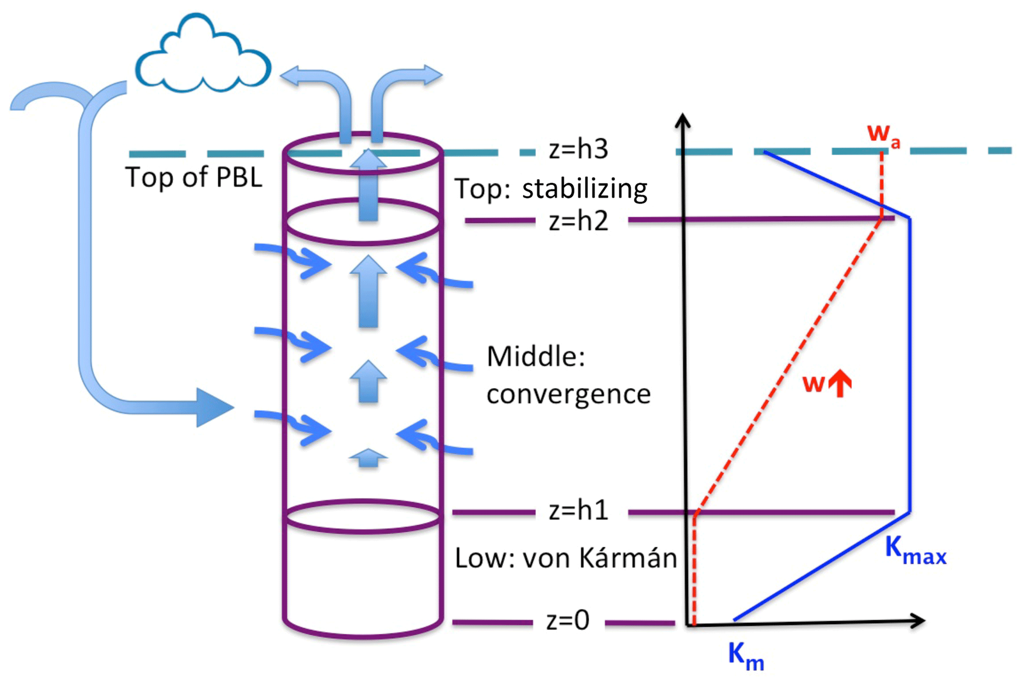
Figure 1Cartoon of the MBL model. The modeled region is indicated by the cylinder. It is comprised of three layers – the low von Kármán layer, the middle convergence layer, and the top stabilizing layer. The heavy straight arrows represent the flow of semi-moist air ascending through the middle and top layers and through the top of the MBL into the free atmosphere (above the model) where clouds and precipitation may form, after which some depleted air from the model column or elsewhere sinks and mixes into the MBL and converges into the middle layer of the model (thin wiggly arrows). Vapor is advected by the vertical motion of air in the middle and top layers and is transported by vertical (diffusive) mixing in all three layers. To the right are graphs of w(z) (dashed red) and K(z) (solid blue) as they vary through the three layers.
Sketched on the right side of Fig. 1 are vertical profiles of the diffusion coefficient K(z) and the (dynamic) vertical velocity w(z). The profile of K(z) is consistent with typical variation with height of the eddy viscosity diffusion coefficient in the boundary layer, based on O'Brien (1970). The coefficient K(z) equals the molecular diffusion coefficient Km at the surface and increases linearly with height to a maximum value Kmax at z=h1. It remains fixed at Kmax through the middle layer, then decreases linearly in the top layer above z=h2 to a small value Kt at z=h3. The vertical velocity w(z) is zero in Layer 1, increases linearly with height through the middle layer, in which convergence occurs at a fixed rate, and remains constant at value wa in Layer 3. Consistent with their constant values of w, Layers 1 and 3 do not have convergence.
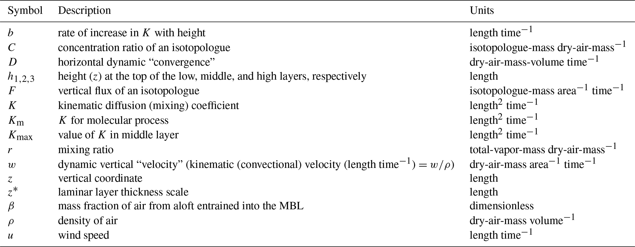
The following Sect. 2.1–2.3 describes the individual physical and mathematical features of the model. Table 1 contains a list of variables and parameters found in these subsections and elsewhere.
2.1 Mixing process
The central matter for this subsection is the specification of the height-dependent eddy diffusion coefficient, Ki(z), which appears in Fick's law for diffusive flux,
where Fi is the vertical flux of the ith isotopologue (isotopologue-mass area−1 time−1), Ci is the concentration ratio of the ith isotopologue (isotopologue-mass dry-air-mass−1), ρ is the density of dry air (mass-of-dry-air volume−1), and z is the vertical coordinate (increasing upwards from z=0 at the surface). The i subscripts of F, K, and C are reminders that they all depend on the specific isotopologue under consideration, but for simplicity we drop them hereafter. We note that Ci has the same units as the commonly used mixing ratio r. The difference is that r is total water vapor mass per unit of dry air mass, while Ci is the mass of the ith isotopologue (e.g., ) per unit of dry air mass. In this paper, we will use the term concentration ratio for C and mixing ratio for r. With Eq. (1), we assume that Fick's law can be used to represent vertical mixing by the combined effects of mechanically driven turbulence, buoyancy-driven convection, and molecular diffusion.
In adopting Fick's law, here, we have made the tacit assumption that alternative mixing models are less appropriate for our purposes. While higher-order closure schemes (e.g., Burk, 1977), structured turbulence models (e.g., Kirwan, 1968), and the telegraph equation (e.g., Goldstein, 1951) have some advantages over Fick's law, their added complexity would not be justified at this juncture, and we postpone their consideration until future investigations warrant.
Conservation of mass for an isotopologue affected only by diffusion, temporarily neglecting convergence and advection, takes the form
For F given by Eq. (1), and for the case of ρ with negligible dependence on z or t, Eq. (2) becomes
Returning to the central matter, the specification of K(z), we reject the assumption of constant K, the simplest and most frequently used assumption, because it is particularly unrealistic near boundaries (i.e., water–air interface in this work), where the inhibitive effect of the interface on mixing of air increases with proximity to the boundary. The next most frequently used assumption is that K is a linear function of z, although a few others have been proposed (Merlivat and Coantic, 1975). The use of linear functions of z to represent K(z) has a long history in turbulence studies, including the turbulent transport of momentum as well as both buoyantly active and passive scalar fluid properties. The well-known work of von Kármán (1930) and Prandtl (1932) successfully applied the simple form , where b is a constant, to derive the equation of the logarithmic layer, where , with u being the wind speed and s and m being constants.
An obvious limitation of the widely cited von Kármán–Prandtl formulation occurs when z is very small, near the singularity at z=0. The most common way to circumvent this problem has been to introduce a discrete “laminar boundary layer” (LBL), a very thin but finite layer with constant diffusion by molecular motion and with weak turbulent influence. The incremental cost of this approach is the necessity of specifying one additional parameter, δ, the thickness of the LBL.
Another way to overcome the problem for small z is to use the more general form
where Km is the molecular diffusion coefficient for vapor in air and b⋅z is the contribution of turbulent eddies to the diffusion coefficient. An equivalent general linear form was applied to boundary layer mixing above the LBL by Montgomery (1940) and within the LBL by Sverdrup (1946, 1951). Note that Km varies among isotopologues, but b does not. This is the basic cause of kinetic fractionation. When z is small (see Eq. 4 and , below), the relative differences among K(z) values for different isotopologues are large, which is the basis for strong kinetic isotopic fractionation near the interface.
One advantage of the form of Eq. (4) for the parameterization is the gain of 1 degree of freedom through the use of the known quantity Km instead of the unknown parameter δ, the thickness of the laminar layer. The latter can be replaced by a diagnostic laminar layer thickness, z*, the height where molecular and turbulent diffusion coefficients are equal. In other words, below z* vertical diffusion is dominated by molecular processes, and above it turbulence and convection prevail. From Eq. (4),
The z* values reported in this paper were computed using the diffusion coefficient of . A linear approach, mathematically equivalent to Eq. (4) (Sheppard, 1958), used bulk aerodynamic theory to modify the work of Sverdrup (1946, 1951). The result was another linear function of z containing the friction velocity u∗ and von Kármán's constant κ instead of the coefficients Km and b, thus connecting Sheppard's model to familiar parameters of fluid mechanics.
Merlivat and Coantic (1975) tested and compared various linear and nonlinear alternatives to Eq. (4). In contrasting alternative boundary layer models for use in isotope studies, they concluded that their laboratory experiments did not support Sheppard's linear theory. However, at the larger scale of Arctic lake field experiments, Eq. (4), which is mathematically equivalent to the approach of Sheppard (1958), was used successfully to model atmospheric vapor isotopes (Feng et al., 2016).
There are several additional benefits to using Eq. (4) rather than parameterizing the kinetic isotopic fractionation. First, K is a boundary layer dynamics parameter that already exists in boundary layer dynamics literature. More importantly, by making kinetic fractionation a function of K(z), our model is capable of exploring how boundary layer mixing affects the kinetic isotopic fractionation. In addition, this formulation allows our model to compute fluxes of isotopologues, not just their ratios, which in turn allows computation of sea surface evaporation. This is significant because the isotopic distribution can then be used to constrain evaporation rate (Feng et al., 2016). Furthermore, with K a continuous function of z, our model is truly one-dimensional, which allows vertical isotopic profiles to be predicted and compared with isotopic observations at multiple heights and with any resolution (Feng et al., 2016). Hence, we proceed with Eq. (4).
2.2 Convergence and vertical advection
Moist air undergoing the Rayleigh distillation process in the free atmosphere is generally conceived to have originated in the PBL and been lifted (i.e., vertically advected) into the free atmosphere. For mass to be conserved, such uplift must be accompanied by convergence within the PBL. Nevertheless, C–G-type models ignore convergence within the boundary layer (e.g., Craig and Gordon, 1965; Merlivat and Jouzel, 1979). The incorporation of this apparent contradiction into a model might be justified by arguing that the effect of boundary layer convergence on isotopic processes is negligible or if the only concern is the isotopic evolution of the liquid where the vapor originates. In the IMBL model presented here, however, we choose to preserve consistency by including both convergence and uplift and to use model results to diagnose the importance of the convergence effect rather than neglecting it a priori. As we later show, convergence has a large influence on the isotopic composition of the air exiting the MBL upward into the free atmosphere.
Steady-state conservation of mass for dry air, using dynamic variables and neglecting diffusion, can be written in the form
where D (here considered independent of z) is the horizontal dynamic convergence (dry-air-mass volume−1 time−1), and w(z) is the dynamic vertical velocity (dry-air-mass area−1 time−1), which is positive for upward air movement. The kinematic (conventional) velocity (length time−1) is the dynamic velocity divided by the air density, ρ. Equation (6) indicates when D is positive, w increases upward. We will use Eq. (6) to derive the governing equation for the middle layer in Sect. 2.3.2.
Ignoring (for now) the effect of diffusion, conservation of mass for isotopologues affected only by kinematics can now be expressed as
where CC is the concentration ratio of the isotopologue of the MBL air converging into the area being modeled. The first and second terms on the right are the direct effect of convergence (replacement of air of concentration ratio C by converging air of concentration ratio CC) and the effect of vertical advection, respectively. Note that Eq. (7) is also consistent with the assumed absence of non-divergent horizontal advection.
The converging air, with concentration ratio CC, is a mixture of two air types, with fractional presence by mass β and (1−β), respectively: (1) air from aloft, originally with concentration ratio CE, that has been recently integrated into the MBL by sinking or mixing, and (2) air that has been in the MBL for considerable time and has become essentially identical in properties to the modeled air with concentration ratio C. Thus, and Eq. (7) can be written in terms of CE as
2.3 Governing equations
To find the general form of the steady-state equation of conservation of mass for each vapor isotopologue, we combine the diffusive (Eq. 3) and kinematic (Eq. 8) effects and set :
(Since dynamic variables are used here, this result does not depend on the commonly invoked isopycnal approximation.)
Equation (9) is the general form of the basic governing equation that we solve in layers in which K(z) and w(z) change. This governing equation is implemented three times, once for each isotopologue, with K differing among isotopologues. Equivalently, it may be viewed as a single vector equation of length 3, with each component describing mass conservation for one isotopologue. The method devised here to solve Eq. (9), described in Sect. 3.2, uses the latter strategy.
We now proceed to adapt Eq. (9) to the atmospheric conditions specific to Layers 1–3 – the low, middle, and high layers – of the MBL.
2.3.1 Low layer equation
In the low layer, as described at the beginning of this section and as illustrated in Fig. 1, there is no convergence or uplift. Hence D=0 and w(z)=0. As specified by Eq. (4), K increases linearly with height, from the small molecular value Km at the surface (z=0) to the larger mixing rate Kmax at z=h1, the top of the low (von Kármán) layer, where
In the low layer, Eq. (9) thus simplifies to
2.3.2 Middle layer equation
In the middle layer, where , K(z) is constant and equal to Kmax, and the convergence rate D is also constant. Defining wa as the upward velocity at the top of the middle layer, h2, Eq. (6) implies that w(z) increases linearly from w=0 at z=h1 to w=wa at z=h2, i.e.,
Equation (9), after substituting Eqs. (12)–(13), simplifies to
Within the middle layer, vertical mixing (the first term in Eq. 14) is controlled by the constant eddy diffusion coefficient, Kmax, which is the maximum value of K. The second term in Eq. (14) describes the direct effect of convergence of external air from aloft, originally with concentration ratio CE, into the profile. Vertical advection (the third term) occurs at a rate depending on the linearly increasing velocity and the gradient of C.
2.3.3 High layer equation
The upper layer of the MBL, just below the very top, is often capped by a stable inversion in which diffusion plays a minimal role. Uplift, however, continues upward unabated through the inversion into the free atmosphere, where further evolution of the air mass is beyond the scope of the IMBL model. In the upper layer of the MBL, we assume that K(z) decreases linearly from Kmax at z=h2 to Kt at the top of the MBL (z=h3) and that there is no further convergence, so w(z) here equals wa. Equation (9) thus becomes
3.1 Analytic solutions
All three governing equations, Eqs. (11), (14), and (15), are second-order linear ordinary differential equations with non-constant coefficients. Equations (11) and (15) are homogeneous, while Eq. (14) is inhomogeneous by virtue of CE. Each equation has an analytic solution with two constants of integration, totaling six constants requiring six boundary conditions (BCs). The six BCs are that
-
C(0) is in equilibrium with the surface water. (BC1)
-
C(z) and KdC∕dz are continuous across z=h1. (BC2–3)
-
C(z) and KdC∕dz are continuous across z=h2. (BC4–5)
-
dC∕dz=0 at z=h3. (BC6)
In the low layer, the solution of Eq. (11) is
From (BC1), the constant C0 is the isotopologue concentration ratio in equilibrium with the liquid sea surface at the sea surface temperature (SST) (Horita et al., 2008), which we obtain from the specified isotopic composition of ocean water and the fractionation factors between liquid water and vapor (Majoube, 1971). Kinetic fractionation is caused by vertically distributed molecular processes concentrated mostly between the surface and and is explicitly included by the presence of Km in Eq. (16). This treatment of kinetic fractionation, alone, distinguishes between this IMBL and most other models of atmospheric vapor isotopes near the sea surface.
The second constant of integration in Eq. (16) is C1, which is the value of C(z) at z=h1. This constant cannot be evaluated at this point, but we return to it shortly.
Similar to the low layer, the middle and high layers have analytic solutions. As is standard with boundary condition problems, the general solutions are found first. Then BC2–5 are introduced into the solutions, and the four new constants of integration are solved for (in terms of the model parameters). The results are given in Sects. S1 and S2 in the Supplement.
The solutions given by Sects. S1 and S2 are long expressions that are far less amenable to evaluation and interpretation than Eq. (16), their equivalent for the low layer. Furthermore, they still contain constants C0 and C1, introduced from Eq. (16) via the BCs for continuity at z=h1. Thus, the solutions for the middle and high layers cannot be evaluated until after C1 has been found.
In order to find C1, it is necessary to apply (BC6) to equations in Sects. S1 and S2. The somewhat lengthy result is the equation in Sect. S3. Once C1 has been evaluated, it is feasible (but tedious and slow) to evaluate equations given in Sects. S1 and S2 along with Eq. (16), completing the evaluation of the unique solution set.
3.2 Hybrid analytical–numerical solutions
It is more convenient to use a hybrid analytical–numerical approach to finding the solution set. The simple analytic solution for the low layer (Eq. 16) can be evaluated in conjunction with a numerical solution for the middle and high layer equations (Eqs. 14 and 15).
Numerical boundary value problem solvers normally require the specification of boundary conditions containing only the variables, their derivatives, and numerical constants. Such a solver would not be of use here because the constant C1 is not known a priori, so BC2 and BC3 cannot be invoked. However, MATLAB's© boundary value problem solver bvp5c offers the option of specifying one unknown “parameter” together with two second-order boundary value problems and five (instead of the usual four) boundary conditions and solving for the unknown parameter as well as the continuous variables. In the analytic problem, this would be equivalent to using five boundary conditions to solve for four unknown constants of integration and one unknown parameter (C1), essentially what was described in Sect. 3.1.
The MATLAB© function PBL_analy_numer, in Sect. S4, uses this technique to solve for the isotopologue profiles in the MBL. It calls the solver bvp5c (line 143). The solver bvp5c, in turn, calls the function res (line 416), for the boundary conditions. Since C1 appears in BC2, it can be designated by res as an “unknown parameter”, and the five other boundary conditions (BC2–6) can be specified. The boundary value problem that governs the isotopologue profiles in the MBL is thus completely determined.
3.3 Summary
Table 2 contains a list of the eight model parameters that must be specified based on environmental information and the eight model outputs (either prognostic or diagnostic variables) that are routinely calculated by the model (others can be added). Remember that C is a vector of dimension 3, corresponding to three isotopologues.
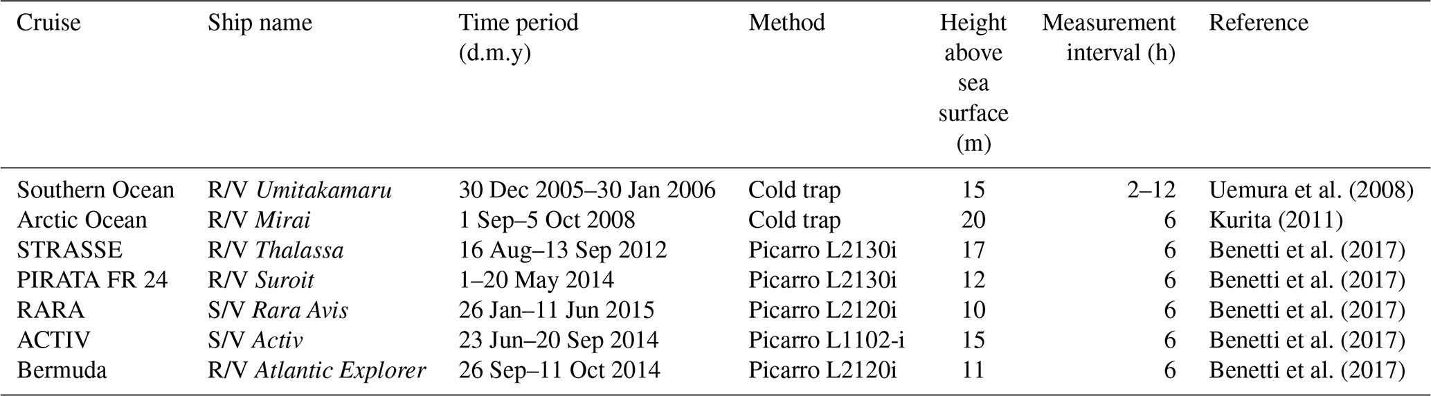
We use seven published data sets for verification of and comparison with our model output. All of these data sets were collected by shipboard measurements. The summary information is included in Table 3, and cruise tracks are illustrated in Fig. 2. Samples from these cruises cover a wide range of the world oceans, from the Arctic Ocean to the northern coast of Antarctica. For earlier data sets, i.e., those by Uemura et al. (2008) and Kurita (2011), samples were collected by the cold trap method, and each sample represents an average of 2–12 h of vapor trapping. Data from the latter five cruises reported by Benetti et al. (2017) were collected by isotope vapor analyzers with the reported instrument model included in Table 3. Benetti et al. (2017) published data sets with either 15 min or 6 h resolutions; the 6 h average data are used for this work. The sea surface temperature (SST), which was either directly measured or estimated by the authors, is reported in all data sets. The relative humidity with respect to SST, RHSST, is either reported (Benetti et al., 2017) or can be calculated based on the measured air temperature and relative humidity at the sampling height. Both SST and RHSST are important variables in our model validations.
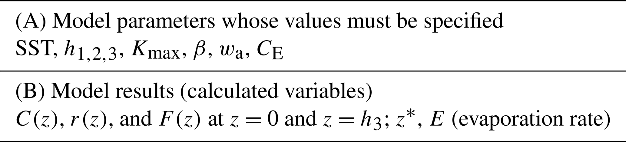
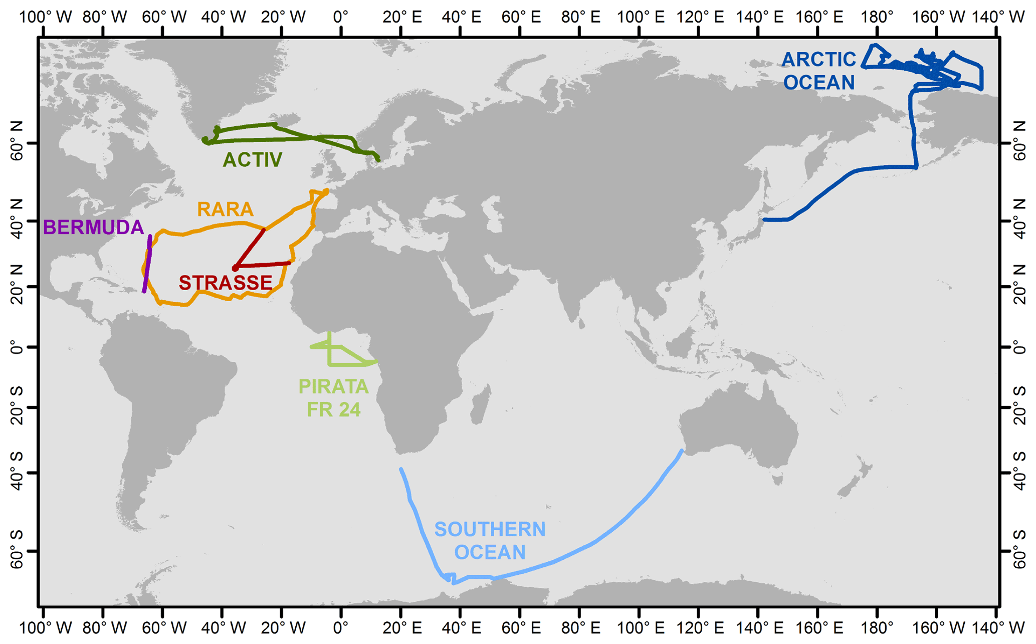
Figure 2Map showing the tracks for seven cruises that generated vapor isotopic observations used in this work. Information about each cruise is listed in Table 3 and the associated references.
Table 3Source of data sets used for validation of the IMBL model.
In this section, we discuss the ranges of parameter values used in the IMBL model verification simulations. The values are summarized in Table 4.
Table 4Parameter values used in model verification simulations.

5.1 Sea surface temperature (SST)
The range of SST used in the simulations was from −2 to +30 ∘C, covering the range of the cruise data sets in Table 3.
5.2 Heights
A finite span of values was not used for either h2 or h3 because results are insensitive to both, and computations were thus reduced in number. The single value used for the MBL height (h3) was 1000 m, a typical MBL height (Stull, 1988), especially in convergent vapor source areas. Similarly, 650 m was the only value used for h2. Conversely, a full range of values was used for h1 because an informal survey of marine radiosonde data suggests that h1 may range from 50 to 200 m and our results are sensitive to the value of h1.
5.3 Eddy diffusivity Kmax
The eddy diffusivity, K, in the atmosphere boundary layer varies widely over many orders of magnitude. Stull (1988) cited values from 0.1 to 2000 m2 s−1, with typical values on the order of 1 to 10 m2 s−1 for the atmosphere boundary layer. Olivié et al. (2004) presented a calculated range of 0.01 to 3000 m2 s−1 in the lowest 3 km of the atmosphere for 15 days in July 1993 at two continental and one marine location; their maximum value (Kmax) above the Pacific Ocean location ranged from about 3 to 300 m2 s−1. Holtslag and Boville (1993) reported calculated zonal and 31-day average eddy diffusivities between 60∘ S and 60∘ N; Kmax ranged from 20 to 60 m2 s−1. For Kmax greater than 10 m2 s−1, model isotopic ratios change only negligibly. At Kmax values less than 1 m2 s−1, the kinetic isotopic fractionation increases significantly as Kmax decreases. We therefore use a Kmax range from 0.01 to 100 m2 s−1 to obtain the full extent of kinetic fractionation.
5.4 Properties of subsiding air (rE, CE, β)
Modeling of convergence requires knowledge of the mixing ratio of the descending air (rE in grams of vapor per kilogram of dry air) and its isotopic compositions (CE), as well as its proportion (β) in the air converged into the MBL. Recall that CE is a vector of length three, corresponding to the concentration ratios of the three modeled isotopologues. The CE value of is only very slightly less than rE, while values of CE for the other two isotopologues can be obtained from rE and isotopic ratios (δD and δ18O) of the vapor.
Vertical profiles of rE over the ocean have been well observed. We used standard resolution radiosonde data from the University of Wyoming (http://weather.uwyo.edu/upperair/sounding.html, last access: October 2015) to examine typical tropospheric values and vertical profiles of the mixing ratio. Generally, the mixing ratio decreases rapidly with height within the lower troposphere and becomes quite small above the midtroposphere. Subsiding air originating in the high troposphere has a correspondingly low mixing ratio. For example, at 500 hPa, the summer-averaged mixing ratio value in the ECMWF (European Centre for Medium-Range Weather Forecasts) data varies from 0.5 to 2 g kg−1. Most cruise data in Table 3 were obtained between summer and fall, particularly the high-latitude ones, and we thus use a range of 0.5–2 g kg−1 for rE (Table 4) in the simulations.
Measurements of the isotopic composition of vapor are scarce at high altitude. Worden et al. (2007) determined the isotopic composition of tropospheric water vapor from global satellite observations. Values of δD averaged over the altitude range corresponding to pressures between 800 and 550 hPa were found to vary from −180 ‰ to −250 ‰ over the extratropical ocean. A more recent update reported δD values from −140 ‰ to −250 ‰ between 900 and 425 hPa (TESv5 from Sutanto et al., 2015). The measurements of Ehhalt (1974) from aircraft above the Pacific Ocean offshore of Santa Barbara, California, showed vertical variations in δD from −96 ‰ to −462 ‰ between 15 and ∼10 000 m for all seasons. The averages for all seasons range from −205 at 800 hPa to −303 ‰ at 550 hPa. The range of Ehhalt's data is lower but overlaps the range of satellite values (Worden et al., 2007; Sutanto et al., 2015). There are no corresponding measurements of δ18O. For the verification simulations, we use a representative value of −239 ‰ for δD and −33 ‰ for δ18O (Table 4). Although this choice is somewhat arbitrary, we show that it is adequate for most cruise data sets. To demonstrate the effect of this value, we also show model results with δ18O of −28 ‰as a comparison.
The proportion, β, of midtropospheric air within air converged into the modeled column of the MBL varies with atmospheric conditions including MBL stability, wind speed, and surface roughness. We use a range of values for β from 1 % to 10 %, which are conjectured values, in the verification simulations.
5.5 Upward velocity (w∕ρ)
NCEP/NCAR reanalysis data (Kalney et al., 1996) show that the upward velocity at 850 hPa ranges globally from 0.01 to 0.4 Pa s−1 in magnitude. A typical value of w is 0.1 Pa s−1 over the ocean in summer. Higher values of upward velocity can be driven by deep convection, which may, in turn, be driven by long-wave radiative cooling at cloud tops, for example. However, the sensitivity of MBL isotopic ratios to w decreases with larger w. We thus use a range from 0.012 to 0.18 Pa s−1, corresponding to 0.01 to 0.15 m s−1.
5.6 Other parameters and constants
In addition to the parameters discussed above, a few more parameters and/or constants are needed for the simulations. For the isotopic compositions of ocean water, both δD and δ18O are set to zero. The molecular diffusivity of in air is assumed to equal that of bulk water vapor, whose temperature dependence in square meters per second is given by the polynomial fit to the data of Bolz and Tuve (1976) (Nellis and Klein, 2009), . The molecular diffusivities of and HD16O are both smaller than that of by factors of 0.9723 and 0.9755, respectively, based on values of Merlivat (1978). The turbulent diffusivity at the top of the MBL is set to 100 Km; while there are few data with which to justify this choice, it suffices because the results are insensitive to it.
The values listed in Table 4 yield 2835 combinations, the result of which is the set of model results we discuss in the next section.
In this section, we discuss the characteristics of the model output and their physical significance and compare the output with observations. We first show vertical profiles of isotopic properties of vapor in the MBL for a representative set of parameters, and then we present the entire set of results of 2835 calculations. These results are then compared with cruise data in both δD vs. δ18O, and d-excess vs. δ18O spaces. We end the section with a discussion of model limitations and potential future developments.
6.1 Characteristics of model results and model validation
While a full discussion of parameter sensitivities and the associated physical processes is the subject of an anticipated companion paper, we point out a few major features of the model output that will guide our discussion of model validation. We start by presenting vertical profiles of δD, δ18O and d-excess. We do so to emphasize that this model is a true 1-D model, unlike models of the Craig–Gordon type. We also emphasize the points that (1) there are strong gradients near the air–sea interface and (2) all isotopic vapor observations made during marine research cruises are performed at a single height, corresponding to just one point of each of the δD, δ18O, and d-excess profiles. We then discuss the δD–δ18O and d-excess–δ18O relationships, which are of major importance to the isotopic interpretation of vapor and precipitation (both modern and ancient such as tree rings and ice cores).
6.1.1 Vertical profiles
As a one-dimensional model, the IMBL model yields the vertical distribution of the isotopic quantities δD, δ18O, and d-excess (= δD–8δ18O). Figure 3 illustrates a typical result. Vapor isotopic values δ18O and δD are both high near the sea surface, where vapor is in equilibrium with ocean water. With increasing height, isotopic ratios and humidity decrease because of the mixing of MBL vapor with isotopically depleted vapor that descends from the upper atmosphere outside, and then is converged into, the modeled column. The upper atmosphere vapor has much lower values of both δD (−239 ‰) and δ18O (−33 ‰), but a higher value of d-excess (25 ‰), than vapor in equilibrium with ocean water.
The profiles in Fig. 3 display strong curvature with very steep gradients near the sea surface, diminishing to negligibly small gradients throughout the MBL. This curvature arises from the rapid change in K from very small molecular values within the thin laminar layer near the water–air interface to large turbulent values above the laminar layer. In this work, the thickness of this layer is characterized by z*, the height of the crossover between molecular and turbulent diffusivities, below which turbulent diffusion is suppressed (see Eqs. 4 and 5).
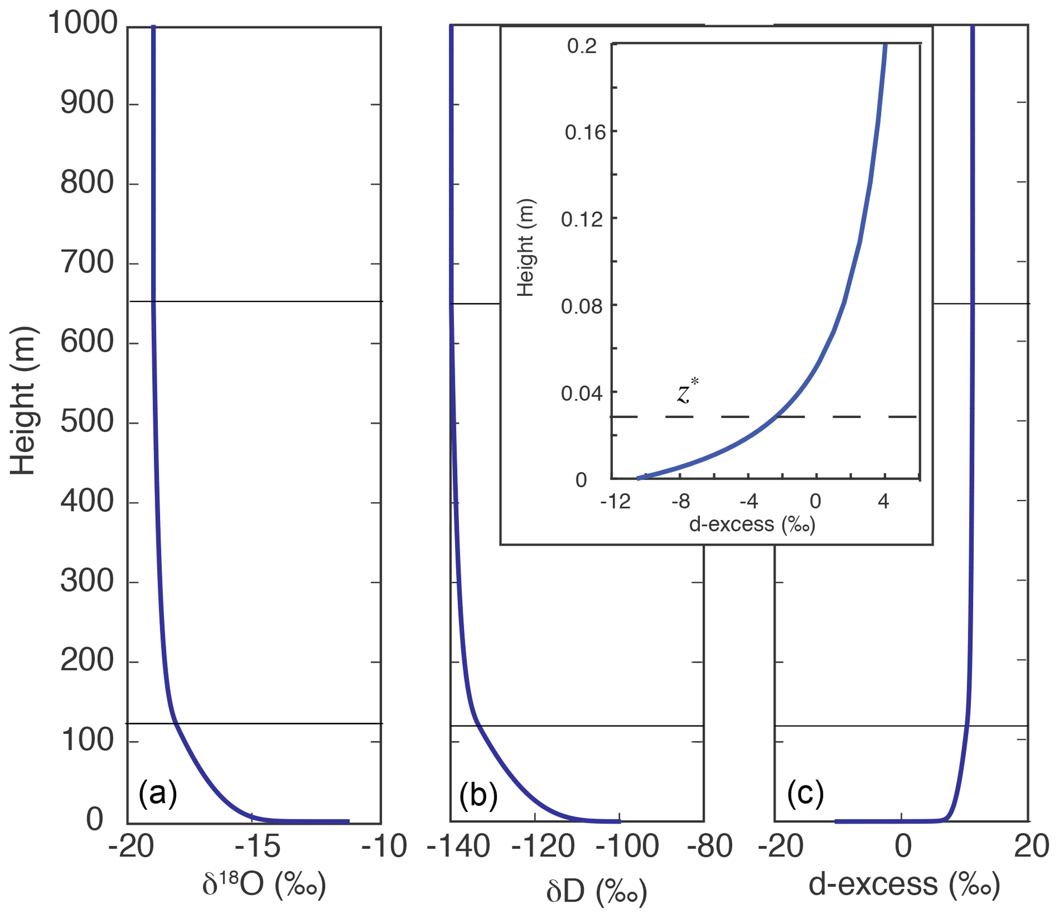
Figure 3Model simulation of vertical distributions of δ18O (a), δD (b), and d-excess (c). Parameters are SST = 5 ∘C, Kmax=0.1 m2 s−1, h1=120 m, rE=0.5 g kg−1, wa=0.15 m s−1, and β=0.05, and δ18O, δD, and d-excess of subsiding air are −33 ‰, −239 ‰, and 25 ‰, respectively. The horizontal solid lines mark the heights of h1 and h2 (120 and 650 m). The inset graph shows d-excess variation with height in the 20 cm just above the sea surface. The dashed line marks the value of z* (0.027 m), below which molecular diffusion is more significant than turbulent diffusion.
The small molecular diffusivity that dominates diffusion in the laminar layer – in particular its differences among isotopologues – is the cause of kinetic fractionation. Kinetic isotope fractionation is reflected by d-excess that changes more sharply near the surface than either δD or δ18O. The smaller inset of d-excess vs. height plot shows variations within 20 cm of the water–air interface. The z* value, which is 2.7 cm in this particular run, is indicated in the inset by the dashed line. The effect of turbulent diffusion increases with height, and thus the rate of change in d-excess with height decreases rapidly as the height increases.
Most in situ observations are conducted at a fixed height above the sea surface. The seven cruise data sets (Table 3) were collected at heights between 10 and 20 m. In these cases, each measurement represents an air sample at a given height along a vertical profile. As shown in the calculation depicted in Fig. 3, isotopic gradients are greatest near the sea surface; in this example, over just 15 m (which is only 1.5 % of the total height of the MBL) δ18O, δD, and d-excess achieve 58 %, 43 %, and 88 %, respectively, of the change toward the relatively constant values between h2 and h3 (650–1000 m). Above 10 m, isotopic change with height is relatively slow. For example, in this particular calculation, at 15 m the δ18O, δD, and d-excess values are −15.6 ‰, −112.6 ‰, and 12.2 ‰, respectively; they change by only 0.50 ‰, 3.56 ‰, and 0.40 ‰, respectively, between 10 and 20 m. Consequently, the isotopic variations between 10 and 20 m to be discussed in the upcoming sections can be viewed as approximating the isotopic variations in vapor delivered to the free troposphere. If the actual vapor isotopic ratios of an air mass to initiate a Rayleigh process are desired, the values at h3 should be used.
6.1.2 The δD vs. δ18O relationship
Each of the 2835 combinations of parameter values described previously was used for one model run. Isotopic ratios were calculated at 15 m above the sea surface and plotted in δD–δ18O space (Fig. 4, main graph). The choice of 15 m in height for Fig. 4 is somewhat arbitrary but is approximately the average of the observation heights, which range from 10 to 20 m, in the seven data sets with which we compare our results (Table 3). In the upper small inset, superimposed in red over the 15 m values are isotopic ratios at both 0 m (in equilibrium with seawater at 5 ∘C) and 15 m for the particular simulation presented in Fig. 3, giving a different perspective on the vertical isotopic change. Vapor at 15 m for this particular run has about average deviation from the sea surface equilibrium vapor. Other runs may have larger or smaller vertical gradients in either or both δD or δ18O. The magnitude of the vertical gradient is reflected by the value of z*. Among the 2835 runs, the distribution of z* is right skewed with a range from 0.001 to 52 cm and a median of 2.8 cm. This median z* value is similar to and thus well represented by the particular run in Fig. 3 ( cm). As discussed earlier, most changes occur below 10 m; above 10 m the change in isotopic composition is relatively minor.
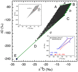
Figure 4δD vs. δ18O relationship at a height of 15 m for 2835 model calculations (+). The output defines a quadrilateral with corners labeled A–D. Also shown are δD and δ18O values of the descending air (E, ⧫) and isotope values of vapor in equilibrium with the seawater (green □, along line b) at SSTs of −2, 5, 10, 15, 20, 25, and 30 ∘C from C to B. Solid lines labeled a, b, and c bound the theoretical limits of vapor isotopic values, with b being vapor in equilibrium with seawater, c being a mixture of vapor at the sea surface and vapor from aloft, and a indicating vapor produced by maximum kinetic fractionation. The upper small inset replicates in gray the 2835 points from all calculations (+), plus red solid dots to indicate vapor isotope values at 0 and 15 m above the sea surface for the run illustrated in Fig. 3. The lower small inset compares two quadrilateral regions produced by assuming different δ18O values of the descending vapor. The blue area with labels A–E is identical to the main graph, and the red quadrilateral corresponds to descending air composition of −28 ‰.
The lower small inset in Fig. 4 shows a comparison of two sets of simulations (2835 runs each) using different oxygen isotopic ratios for the upper atmosphere air. Only the boundaries of the output areas are shown, with blue being identical to the main graph and red indicating the range of results produced using −28 ‰ (rather than −33 ‰) for the δ18O value of the upper atmosphere vapor.
The output in δD–δ18O space (Fig. 4) defines a quadrilateral with each corner labeled A through D. The edges (BC, CD, DA, and AB) have specific physical significance. Line BC (line b) connects all points (squares) representing isotopic values of vapor in equilibrium with seawater, for the range of sea surface temperatures considered. With increasing sea surface temperature, the points shift from lower left (C) to upper right (B). Points close to this line reflect model parameters that permit very little kinetic isotopic fractionation to occur between the sea surface and 15 m and very little influence of descending air (whose isotopic composition is point E). Close examination reveals that the points near line BC were generated with the largest turbulent mixing coefficients (highest Kmax) and a very small fraction of external air (small β∼0.01). Consequently, z* values are very small ( m), and the relative humidity with respect to SST, RHSST, is close to saturation, both of which are responsible for the small degree of kinetic isotopic fractionation. Large Kmax also creates a well-mixed MBL, which is consistent with the simulated low isotopic gradients between the sea surface and 15 m.
Line CD bounds points that have the smallest deviation from the straight line CE (line c) that represents mixing of vapor in equilibrium with SST at the coldest temperature considered (−2 ∘C, point C) and vapor from the descending high-altitude dry air (E). Increasing contribution from kinetic isotopic fractionation moves points increasingly above this line (see further discussion below). Therefore, points on this line represent no kinetic fractionation, with the influence of upper atmosphere air increasing from C to E. In other words, if the SST is −2 ∘C, line CE represents a lower bound on isotopic mixing. At a fixed SST and ocean isotopic ratio, this line rotates with changing isotopic ratios in the air aloft, for example, line CF in the lower inset of Fig. 4. Similarly, mixing lines between equilibrium vapor at higher SSTs should be straight lines connecting point E and points along line b representing vapor in equilibrium with seawater at different temperatures. For example, if the SST is 30 ∘C, then the mixing line would be BE (not shown), and all isotopic ratios of vapor evaporated from this sea surface should be above this line.
The points along line AB represent vapor evaporated from ocean water at SST = 30 ∘C. Their spread reflects the influence of kinetic fractionation; moreover, they are not significantly influenced by mixing with upper atmosphere air. This inference is supported by their small values of Kmax (0.1 m2 s−1), large z* (0.3–0.5 m), and low rE of the upper atmosphere (0.5 g kg−1). Theoretically, the slope of AB should have a limit of 0.88 (shown as line a), the ratio of the kinetic fractionation factors of HDO and (25.1 ‰ and 28.5 ‰, respectively, because and 1.0285, respectively, where the star represents the heavy isotopologue; Merlivat, 1978). With the set of parameters in Table 4, the slope of AB is about 1.5, slightly greater than its lower limit (0.88). Therefore, line a sets the upper bound for vapor isotopic ratios for an SST of 30 ∘C. In other words, the theoretical limit for the highest isotopic ratios at a given SST should be along a line that starts from a point representing vapor in equilibrium with seawater (δ18O = 0, δD = 0 in this calculation) at this temperature and extends to the lower left with a slope no less than 0.88.
Line AD bounds isotopic compositions reflecting the entire range of SST values; both kinetic fractionation and mixing with the upper atmosphere have significant influences on these points. The ambient conditions are characterized by small Kmax (0.01 m2 s−1), large β (0.1), and relatively high z* values (0.1–0.5 m). This AD “line” is not as strictly defined as other lines in that it does not have an absolute theoretical limit and so may change with the range of parameter space. In subsequent discussion, we refer to line a as the upper limit, line b as the side limit, and line c as the bottom limit of the vapor distribution in the δD–δ18O space, consistent with their positions in Fig. 4.
In summary, the shape of the output in Fig. 4 is controlled by three factors, (1) the SST, (2) the degree of kinetic isotopic fractionation, and (3) the influence of upper atmosphere air. While SST is relatively independent of other factors, kinetic fractionation and the effect of upper air depend on various combinations of atmospheric conditions, including the intensity of turbulent mixing (Kmax), the mixing ratio of the descending air (rE) and its isotopic ratios, the proportion of upper atmospheric air advected into the evaporation column (β), and the vertical velocity (w). Note that in this model, the relative humidity with respect to SST (RHSST) is not, and cannot be, prescribed. On the contrary, it is an outcome of the same meteorological conditions of the MBL that affect the isotopic ratios, although it also feeds back on kinetic isotopic fractionation by controlling the vertical gradient for vapor diffusion.
Model output and observational data for each individual cruise are compared in Fig. 5. Model output is calculated at the observation height of the corresponding cruise, indicated in the graph. Also included in each plot are compositions of vapor in equilibrium with seawater at the lowest and highest SSTs of the cruise. The theoretical borders under specific cruise conditions are shown as solid lines; observed isotopic ratios are expected to fall within these theoretical limits (if consistent with the assumed ocean water and descending air isotopic ratios).
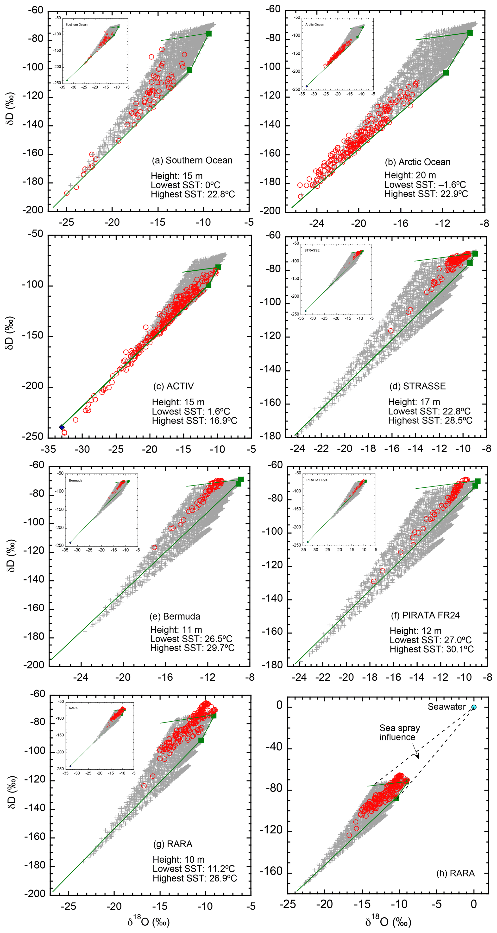
Figure 5Comparisons between simulated and observed isotopic ratios for each of the seven cruises (a–g), and a redraw of the RARA data with ocean water composition indicated (h). For each cruise, the simulated values are calculated at the height of the observations, indicated in the plot. If not otherwise indicated, calculated isotopic values are shown as crosses (+), the values of the descending air as a diamond (⧫), and observations as red circles (◦). For each cruise, vapor in equilibrium with lowest and highest SSTs is shown as two green squares (▪), with the temperature values indicated in the plot. Solid lines border the theoretical limits of isotopic distributions under the cruise conditions and model assumptions. For (a–g), unless the depleted, descending air is indicated in the main graph by a blue diamond (all but c) it is shown in the insert.
We make the following observations of Fig. 5. First, the vast majority of the observed data (∼95 %) do indeed fall within the expected range. This confirms not only the successful conceptualization of the model but also that our choices of parameter values are reasonable.
Second, in all seven data sets, the influence of the isotopically depleted vapor from descending air is demonstrated by points with low isotopic ratios. These compositions are difficult to model using C–G-type models, particularly with the invalid closure assumption (e.g., Jouzel and Koster, 1996; Benetti et al., 2015). This result highlights the importance of convergence in affecting boundary layer vapor isotopic ratios, as it introduces dry, depleted air from aloft into the MBL. Such influence of upper atmosphere air on the boundary layer has been recognized by Benetti et al. (2015, 2018), although for quiescent subsidence regions that our model does not treat.
Third, for the ACTIV cruise (Fig. 5c), a number of points fall below the lower limit, suggesting that the isotopic ratios of the descending air we used for the simulation may not be representative in this area during the observation period. The mismatch suggests a value that is more enriched in 18O, or depleted in deuterium, or both, than the values used for the simulation.
Fourth, in four cruises (PIRATA, STRASSE, Bermuda, and RARA; Fig. 5d–g), there are points that are above the upper limit. However, in all cases except RARA, the enrichment above the upper limit is small in magnitude and may be explained by slight variations in seawater isotopic ratios. For RARA, however, the enrichment above the upper limit is significant. One possible explanation is the influence of sea spray. When describing the sampling conditions, Benetti et al. (2017) particularly noted that they could not completely rule out the contribution of small droplets of sea spray to the vapor composition. However, such an influence seems relatively small considering the great leverage of seawater isotopic composition. Figure 5h shows the direction and magnitude of sea spray influence; the mixing of sea spray droplets should cause enrichment such that the data would be distributed in the triangular area bordered by the dashed lines. Detailed examination of cruise logs in the future will be helpful to confirm and quantify the sea spray contribution to MBL vapor.
In summary, by comparing calculated values and observational data in δD–δ18O space, we conclude that the model is remarkably successful. We pointed out three factors that may cause observations to fall outside the predicted range, namely (1) variation in ocean water isotopic ratios, (2) variation in the isotopic ratios of the upper atmospheric vapor, and (3) influence of sea spray on vapor isotopes. In Sect. 6.2, we discuss several other model assumptions that may limit the consistency between model results and observations.
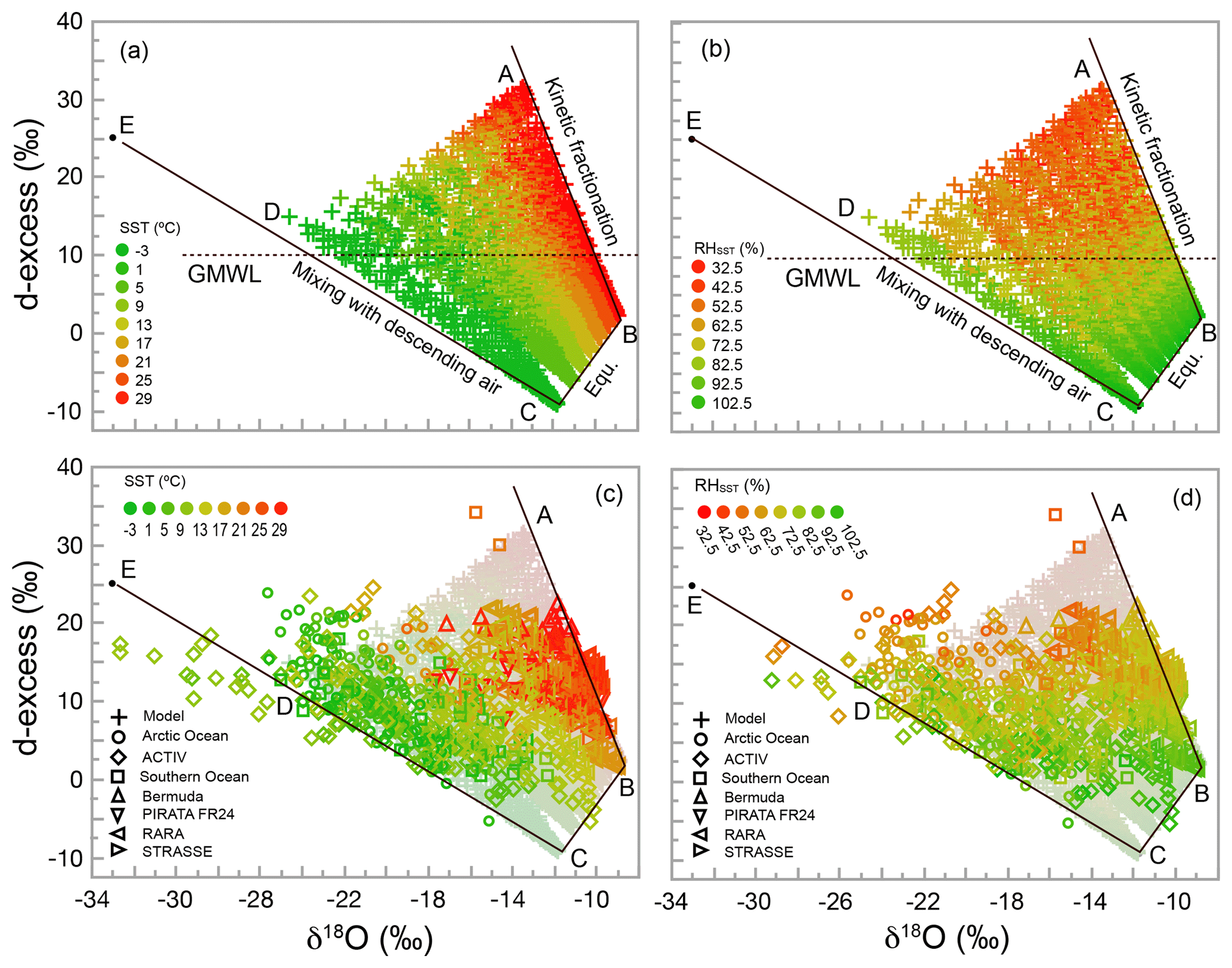
Figure 6Plots of d-excess vs. δ18O, showing the relationship between d-excess and SST for the simulation (a) and model–data comparison (c) and between d-excess and RHSST for simulation (b) and model–data comparison (d). As in Fig. 4, isotopic values are calculated at a height of 15 m. Points corresponding to those from A to E in Fig. 4 are also shown, with point E being the isotopic composition of the descending air. Straight lines are theoretical limits for processes labeled in (a) and (b) (also discussed in Sect. 6.1.2). The horizontal dashed lines in (a) and (b) mark the d-excess value (10) of the global meteoric water line (GMWL).
6.1.3 Deuterium excess (d-excess)
The relationships between d-excess and both sea surface temperature (SST) and relative humidity with respect to SST (RHSST) have been intensively discussed by the isotope hydrology community. Originally defined by Dansgaard (1964) for precipitation as δD–8δ18O, d-excess has been used to infer conditions at the moisture source location. It has been demonstrated that d-excess varies with SST and inversely with RHSST (Johnsen et al., 1989; Petit et al., 1991). Later investigators have used these concepts to infer changes in moisture source conditions recorded in polar ice cores (e.g., Vimeux et al., 1999; Masson-Delmotte et al., 2005a, b).
The relationships between d-excess and SST, and between d-excess and RHSST, are shown in Fig. 6. Our model, as expected, exhibits a significant dependence of d-excess on both SST and RHSST. Regression of d-excess against SST explains 16 % of the variance in d-excess, with a coefficient of 0.35 ‰ ∘C−1. Regression against RHSST explains 78 % of the variance in d-excess, with a coefficient of −0.43 ‰ %−1. These values are very similar to d-excess sensitivities of 0.35 ‰ ∘C−1 to SST and −0.45 ‰ %−1 to RHSST, cited by Vimeux et al. (1999) based on calculations by Johnsen et al. (1989).
All three processes discussed earlier, i.e., changing SST, degree of kinetic fractionation, and extent of mixing with the subsiding air, result in changes in d-excess. This is seen by the fact that the theoretical lines in Fig. 6 representing each of the three processes have nonzero slopes. Although at the sea surface d-excess increases with SST, a much larger spread occurs at 15 m due to the height-dependent influence of the descending air and kinetic fractionation. For each value of SST, the points at 15 m form a triangular area, within which d-excess varies significantly (Fig. 6a). Such a triangular distribution of isotopic data in the d-excess vs. δ18O space has been reported by Steen-Larsen et al. (2015) for observations off the coast of Iceland. This two-dimensional distribution explains the significant, though relatively poor, correlation between d-excess and SST.
Figure 6b shows that the lowest RHSST tends to correspond to the highest d-excess distributed near corner A. However, near point D, where d-excess is also relatively high compared with values at the water–air interface, RHSST is relatively high and kinetic fractionation is limited. Therefore, while d-excess tends to increase as RHSST decreases, the relationship is not one to one (note how color changes horizontally in Fig. 6b). Another way to see this is to trace the color change along lines parallel to CB in Fig. 6a for changes in SST and parallel to AB in Fig. 6b for changes in RHSST. Interestingly, along CD, neither SST nor RHSST varies significantly, regardless of substantial variation in d-excess. Obviously, RHSST is not the sole influence on d-excess, and even the combination of both RHSST and SST does not completely determine d-excess in the MBL.
Data from all cruises are shown in Fig. 6c and d. In order to pool a larger quantity of data, here we ignore the minor differences in sampling heights among the seven data sets. The match between observed and simulated patterns is excellent. First, ∼95 % of data fall within the theoretically predicted region (the percentage may be slightly less than 95 % because the simulation here is performed only at 15 m without considering the sampling height of each cruise). This comes as no surprise given what was already seen in δD–δ18O space (Fig. 5). Factors that cause a small number of observational points to fall outside the predicted region were discussed earlier, and we do not repeat that discussion here. Second, the dependence of the observed d-excess on RHSST and SST, as shown by the color distributions, is very similar to that of model calculations. For SST, the color along lines parallel to CB changes from green to red with a d-excess increase. Similarly, RHSST values are relatively high near lines CB and CE and decrease (with significant noise) towards corner A as d-excess increases. Finally, as predicted, the observed d-excess correlates significantly (p<0.0001) with SST and with RHSST. The sensitivity of d-excess observations to RHSST is −0.36 ‰ %−1, comparing favorably with corresponding model sensitivity of −0.43 ‰ %−1. For SST, the sensitivity for observations is 0.15 ‰ ∘C−1, about half of that predicted by the IMBL model (0.35 ‰ ∘C−1) using SSTs ranging from −2 to 30 ∘C. Detailed discussion of the sensitivity differences between simulations and observations is beyond the scope of this paper, and a full understanding of these relationships should be an important goal for future investigations.
To end this section, we point out that our model–observation comparisons are focused on identifying major processes controlling large-scale isotopic distributions of water vapor. These general comparisons should be followed by simulations specific to given sites over given observation time windows, which would require narrowing down model parameterizations according to the conditions in which and when data were collected. For example, the SST, water isotopic values, vertical velocity, Kmax, and properties of descending air should all be obtained/estimated from either observations or reanalysis products. Such site- and time-specific simulations will allow identification of relative importance of various processes and will lead to an understanding of how the relative contributions of each process vary over space and time. Since such work requires a particular context for each data set, we postpone it to future investigations.
6.2 Model applicability, limitations, and future development
The IMBL model described here has considerable potential value for many isotope hydrology applications. First, as vapor isotopic measurements become increasingly available, application of the model at different locations and times of year provides a vehicle to explore and understand relationships between meteorological conditions and isotopic compositions of vapor both within the MBL and delivered to the free atmosphere. Comparisons of simulations and observations with much more intensive observations than cited in this work may be conducted. For example, during an isotopic vapor measurement campaign, measured variations in the isotopic composition of ocean water and vapor may be combined with model calculations to constrain the diffusion coefficient, which may then be related to sea surface roughness, wind speed, vertical velocity, and sea spray occurrence. Second, the output of this model, i.e., the isotopic ratio of vapor delivered to the free atmosphere, can be used to provide initial conditions for Rayleigh-type condensation or transport models. The sensitivity of precipitation isotopic ratios to the range of meteorological conditions at the moisture source region and their change over time and space can be investigated for modern hydrological cycles in association with atmospheric circulation, as well as under ancient climate conditions. Third, an understanding of physical processes important for controlling the isotopic compositions of water (both vapor and precipitation), gained from these applications, can be used to improve the physical representation of marine boundary layer processes in GCMs.
This IMBL model may not adequately describe several meteorological scenarios, and under those conditions it should be used with caution. First, the model requires that the air column in the model domain have a positive (upward) vertical velocity; i.e., air must be converging and rising. This assumption is made to ensure that the model column represents a moisture source area, delivering vapor to the free troposphere where it will ultimately produce precipitation. If the vertical velocity is negative (i.e., subsiding air), the air in the column diverges rather than converges, meaning that the mass conservation equations used here would not be correct. However, a modest formulation of the governing equations could allow for sinking air (Welp et al., 2018). Either way, the important outcome is that upper atmosphere vapor is incorporated into the MBL. It is possible that isotopic distribution changes somewhat with specific mixing scenario, while the theoretical limits of isotopic distribution remain the same as shown by this work. Second, the model does not include exchange between vapor and liquid if air is supersaturated, forming clouds or precipitating. The model is thus strictly applicable only for meteorological conditions with no cloud base below h3, the top of the MBL (1000 m, here). Third, as discussed earlier, the model does not include the effects of sea spray. Fourth, the modeled column is not subject to horizontal advection (except for convergence). Fifth, the IMBL is a steady-state model.
We envision future improvements in the IMBL model. In particular, we anticipate generalization of the model to include areas of divergence (descending air), areas with sea spray, and/or terrestrial areas. Alternatively, to describe or simulate effects or dynamics of additional boundary layer processes, such as cloud microphysics, researchers could consider using more complex and comprehensive boundary layer models, such as the ISOLESC model (Wei et al., 2018), with associated sacrifice of simplicity.
We have constructed a new isotope marine boundary layer (IMBL) model to calculate the isotopic composition of vapor in the marine boundary layer as well as that of vapor lifted to the free atmosphere. The model divides the MBL into three layers, each with its own transport characteristics. Compared with classical Craig and Gordon (1965) bulk evaporation models, this 1-D (vertical) model makes two improvements. First, it explicitly includes the process of horizontal convergence in the middle layer; convergence provides mass to balance the upward advection supplying moisture for cloud formation and precipitation in the free atmosphere. This formulation requires specification of the properties of subsiding air that mixes with low-altitude air and converges into the model column. Second the eddy diffusion coefficient is height-dependent, equal to the molecular diffusion coefficients for each isotopologue at the air–water interface and increasing linearly through the lower layer to a maximum value, Kmax, remaining constant through the middle layer, and decreasing linearly to Kt over the top layer. The advantages gained from these two improvements include (1) the model solving for both isotopologue concentrations in and fluxes through the MBL, not just fluxes; (2) kinetic isotopic fractionation becoming a diagnostic variable rather than a required parameter, without adding to the total number of parameters (degrees of freedom) of the model; (3) relative humidity also no longer being a specified parameter, but rather becoming a diagnostic variable, thus enabling the use of the model to investigate and possibly predict evaporation rates; (4) calculation of vertical profiles of concentrations and fluxes of isotopologues (or isotopic ratios), providing an opportunity to compare model output with observations at a specific height or multiple heights; and (5) the air at the top of the MBL (at z=h3) being the air mass supplied to the beginning of a Rayleigh trajectory, which can be used for many isotope studies.
The standard output of the model includes vertical profiles of δD, δ18O, and d-excess. Near the sea surface, δD and δ18O are high and close to equilibrium with the ocean water, and d-excess is low. With increasing altitude, δD and δ18O decrease due to both kinetic fractionation and mixing with converging isotopically depleted air that contains subsided air from the free troposphere. Kinetic fractionation near the sea surface causes d-excess to increase rapidly with height, particularly between the air–sea interface and height z*, where molecular diffusion dominates over turbulent mixing.
Model simulations using reasonable ranges of parameters are validated using seven sets of shipboard MBL observations. The resulting range of δD and δ18O forms a quadrilateral-shaped pattern in the δD–δ18O plane. Three processes generate boundaries for the quadrilateral, or constraints on the isotopic ratio distributions, including (1) the set of vapor isotopic ratios in equilibrium with seawater at various SSTs (right side boundary), (2) mixing between vapor descended from the upper atmosphere and vapor in equilibrium with seawater at the air–water interface (lower boundary), and (3) kinetic isotopic fractionation that starts with equilibrium vapor and extends to more depleted values of δD and δ18O, with a slope no less than 0.88 (upper boundary).
About 95 % of observations fall into the theoretically predicted quadrilateral region, demonstrating the success of the model conceptualization and parameter choices. This remarkable agreement highlights the importance of convergence and entrainment of descending, isotopically depleted air to boundary layer isotopic ratios. This feature is new to this model and was not considered in earlier simple models, although some (e.g., Benetti et al., 2015) do include mixing by mathematically unspecified mechanisms other than convergence, in meteorological regions distinct from those we consider. The simulation–observation comparisons also point to at least three factors that may explain the 5 % of data falling outside the predicted region, including (1) variations in seawater isotopic ratios, (2) inaccurate choice of isotopic ratios for the subsiding air, and (3) influence of sea spray. It is also possible that meteorological scenarios not explicitly considered by the model are responsible for the relatively minor model–data mismatch. Such factors may include low-level air divergence (downward vertical velocity in the middle and upper MBL), vapor–liquid exchange (during precipitation events or within clouds), and the presence of lateral advection.
Simulated d-excess compares remarkably well with observations. While the effects of sea surface temperature (SST) and relative humidity with respect to SST (RHSST) are well-understood, we draw attention to the influence of the upper atmosphere air in controlling d-excess in the marine boundary layer. In this simulation, the d-excess value of the descending air is greater than that of vapor in equilibrium with seawater, and the contribution of the former to MBL air results in an increase in d-excess of vapor, even in the absence of kinetic isotopic fractionation. The influence of free troposphere vapor on the d-excess of the boundary layer vapor has also been demonstrated by Benetti et al. (2015, 2018) via a C–G-type approach. Quantification of this influence under various meteorological scenarios should be an important objective for future investigation in order to use d-excess for ice core studies.
The IMBL model can be used in a number of ways. First, numerical experiments with the model help to better understand the effects of boundary layer processes and climatic conditions on isotopic compositions of vapor within and vapor fluxes through the MBL. For example, one may investigate how boundary layer stability, turbulence conditions, vertical velocity, convergence, and upper atmospheric moisture affect MBL isotopic distributions and how these effects change with space and time. A second application could be to investigate how temporal and spatial meteorological differences in moisture source regions affect the isotopic composition of remote precipitation under both modern as well as paleoclimate conditions. In this application, the IMBL model can be coupled with a Rayleigh distillation model to simulate isotopic evolution of vapor and/or precipitation from moisture source to a precipitation site. These simulations can be particularly powerful if also used in conjunction with Lagrangian back-trajectory programs to identify moisture source areas for a site of interest. Third, it is important to investigate the relationship between MBL isotopes and evaporation rate and, perhaps, to develop methods to measure the latter indirectly from simultaneous observations of isotopes and meteorological conditions. Since this IMBL model calculates the flux of each isotopologue (rather than just their ratios), it yields the evaporation rate. This opens up the possibility of using isotopic measurements to quantify evaporation rates under various boundary layer conditions. Finally, the understanding gained from IMBL model simulations can be used to improve the representation of MBL processes in isotope-enabled GCMs.
Observational data can be found from the references in Table 3. Modeling results can be generated using the code provided in the supplemental information and the parameters in Table 4.
The supplement related to this article is available online at: https://doi.org/10.5194/acp-19-4005-2019-supplement.
ESP created and coded the IMBL model, wrote the model description of the paper and edited all other sections. LS helped with coding of the model and intensively edited the paper. XF performed most of the calculations, interpretation of the model output, and drafting of the paper. NF researched model parameters, carried out preliminary sensitivity test of the model, drafted the descriptions of the parameter ranges, and organized part of the data for model validation. All authors were involved in discussions and interpretations of the model results.
The authors declare that they have no conflict of interest.
Funding of this work was in part provided by the National Science Foundation under grant 1022032 for the iisPACS (Isotopic Investigation of Sea ice and Precipitation in the Arctic Climate System) project. We thank Ryu Uemura (personal communication), Kurita (2011), and Benetti et al. (2017) for making their observational data available. Technical assistance by Jonathan W. Chipman is appreciated. We thank the two anonymous reviewers for their thoughtful comments that helped us improve this paper. NCEP Reanalysis data were provided by the NOAA/OAR/ESRL PSD, Boulder, Colorado, USA, from the Web site https://www.esrl.noaa.gov/psd/ (last access: October 2015).
This paper was edited by Thomas Röckmann and reviewed by two anonymous referees.
Andersen, K. K., Azuma, N., Barnola, J. M., Bigler, M., Biscaye, P., Caillon, N., Chappellaz, J., Clausen, H. B., Dahl-Jensen, D., Fischer, H., Fluckiger, J., Fritzsche, D., Fujii, Y., Goto-Azuma, K., Gronvold, K., Gundestrup, N. S., Hansson, M., Huber, C., Hvidberg, C. S., Johnsen, S. J., Jonsell, U., Jouzel, J., Kipfstuhl, S., Landais, A., Leuenberger, M., Lorrain, R., Masson-Delmotte, V., Miller, H., Motoyama, H., Narita, H., Popp, T., Rasmussen, S. O., Raynaud, D., Rothlisberger, R., Ruth, U., Samyn, D., Schwander, J., Shoji, H., Siggard-Andersen, M. L., Steffensen, J. P., Stocker, T., Sveinbjornsdottir, A. E., Svensson, A., Takata, M., Tison, J. L., Thorsteinsson, T., Watanabe, O., Wilhelms, F., White, J. W., and North Greenland Ice Core Project: High-resolution record of Northern Hemisphere climate extending into the last interglacial period, Nature, 431, 147–151, https://doi.org/10.1038/nature02805, 2004.
Benetti, M., Reverdin, G., Pierre, C., Merlivat, L., Risi, C., Steen-Larsen, H. C., and Vimeux, F.: Deuterium excess in marine water vapor: dependency on relative humidity and surface wind speed during evaporation, J. Geophys. Res.-Atmos., 119, 584–593, https://doi.org/10.1002/2013JD020535, 2014.
Benetti, M., Aloisi, G., Reverdin, G., Risi, C., and Sèze, G.: Importance of boundary layer mixing for the isotopic composition of surface vapor over the subtropical North Atlantic Ocean, J. Geophys. Res.-Atmos., 120, 2190–2209, https://doi.org/10.1002/2014jd021947, 2015.
Benetti, M., Steen-Larsen, H. C., Reverdin, G., Sveinbjornsdottir, A. E., Aloisi, G., Berkelhammer, M. B., Bourles, B., Bourras, D., de Coetlogon, G., Cosgrove, A., Faber, A. K., Grelet, J., Hansen, S. B., Johnson, R., Legoff, H., Martin, N., Peters, A. J., Popp, T. J., Reynaud, T., and Winther, M.: Stable isotopes in the atmospheric marine boundary layer water vapour over the Atlantic Ocean, 2012–2015, Scientific Data, 4, 160128, https://doi.org/10.1038/sdata.2016.128, 2017.
Benetti, M., Lacour, J. L., Sveinbjörnsdóttir, A. E., Aloisi, G., Reverdin, G., Risi, C., Peters, A. J., and Steen-Larsen, H. C.: A Framework to Study Mixing Processes in the Marine Boundary Layer Using Water Vapor Isotope Measurements, Geophys. Res. Lett., 45, 2524–2532, https://doi.org/10.1002/2018gl077167, 2018.
Bolz, R. E. and Tuve, G. L.: Handbook of Tables for Applied Engineering Science, 2nd Edn., CRC Press, Boca Raton, Florida, 1976.
Burk, S. D.: The moist boundary layer with a higher order turbulence closure model, J. Atmos. Sci., 34, 629–638, 1977.
Christakos, K., Reuder, J., and Furevik, B. R.: Experimental characterization of the marine atmospheric boundary layer in the Havsul area, Norway, Energy Procedia, 35, 121–127, https://doi.org/10.1016/j.egypro.2013.07.165, 2013.
Craig, H. and Gordon, L. I.: Deuterium and oxygen-18 variations in the ocean and marine atmosphere, in: Stable Isotopes in Oceanographic Studies and Paleotemperatures, edited by: Tongiorgi, E., Spoleto, Italy, 9–130, 1965.
Craig, H., Gordon, L. I., and Horibe, Y.: Isotopic exchange effects in the evaporation of water: 1. Low-temperature experimental results, J. Geophys. Res., 68, 5079–5087, 1963.
Dansgaard, W.: Stable isotopes in precipitation, Tellus, 16, 436–468, 1964.
Dansgaard, W., White, J. W. C., and Johnsen, S. J.: The abrupt termination of the Younger Dryas climate event, Nature, 339, 532–534, 1989.
Ehhalt, D. H.: Vertical profiles of HTO, HDO, and H2O in the troposphere, National Center for Atmospheric Research, Boulder, Colorado, 1974.
Feng, X., Lauder, A. M., Posmentier, E. S., Kopec, B. G., and Virginia, R. A.: Evaporation and transport of water isotopologues from Greenland lakes: The lake size effect, Quaternary Sci. Rev., 131, 302–315, https://doi.org/10.1016/j.quascirev.2015.07.029, 2016.
Feng, X. H., Reddington, A. L., Faiia, A. M., Posmentier, E. S., Shu, Y., and Xu, X. M.: The Changes in North American atmospheric circulation patterns indicated by wood cellulose, Geology, 35, 163–166, https://doi.org/10.1130/g22884a.1, 2007.
Goldstein, S.: On diffusion by discontinuous movements and the telegraph equation, Q. J. Mech. Appl. Math., 4, 129–156, 1951.
Holtslag, A. A. M. and Boville, B. A.: Local versus nonlocal boundary-layer diffusion in a global climate model, J. Climate, 6, 1825–1842, 1993.
Horita, J., Rozanski, K., and Cohen, S.: Isotope effects in the evaporation of water: a status report of the Craig–Gordon model, Isotop. Environ. Health Stud., 44, 23–49, https://doi.org/10.1080/10256010801887174, 2008.
Huang, Y., Shuman, B., Wang, Y., and Webb III, T.: Hydrogen isotope ratios of palmitic acid in lacustrine sediments record late Quaternary climate variations, Geology, 30, 1103–1106, 2002.
Johnsen, S. J., Dansgaard, W., and White, J. W. C.: The origin of Arctic precipitation under present and glacial conditions, Tellus B, 41, 452–468, 1989.
Jouzel, J. and Koster, R. D.: A reconsideration of the initial conditions used for stable water isotope models, J. Geophys. Res.-Atmos., 101, 22933–22938, https://doi.org/10.1029/96jd02362, 1996.
Jouzel, J., Masson-Delmotte, V., Cattani, O., Dreyfus, G., Falourd, S., Hoffmann, G., Minster, B., Nouet, J., Barnola, J. M., Chappellaz, J., Fischer, H., Gallet, J. C., Johnsen, S., Leuenberger, M., Loulergue, L., Luethi, D., Oerter, H., Parrenin, F., Raisbeck, G., Raynaud, D., Schilt, A., Schwander, J., Selmo, E., Souchez, R., Spahni, R., Stauffer, B., Steffensen, J. P., Stenni, B., Stocker, T. F., Tison, J. L., Werner, M., and Wolff, E. W.: Orbital and millennial Antarctic climate variability over the past 800,000 years, Science, 317, 793–796, 2007.
Kalney, E., Kanamitsu, M., Kistler, R., Collins, W., Deaven, D., Gandin, L., Iredell, M., Saha, S., White, G., Woollen, J., Zhu, Y., Chelliah, M., Ebisuzaki, W., Higgins, W., Janowiak, J., Mo, K. C., Ropelewski, C., J., W., Leetmaa, A., Reynolds, R., Jenne, R., and Josheph, D.: The NCEP/NCAR 40-year reanalysis project, B. Am. Meteorol. Soc., 77, 437–471, 1996.
Kirwan, J. A. D.: Constitutive equations for a fluid containing nonrigid structures, Phys. Fluids, 11, 1440–1446, 1968.
Kopec, B. G., Lauder, A. M., Posmentier, E. S., and Feng, X.: The diel cycle of water vapor in west Greenland, J. Geophys. Res.-Atmos., 119, 2014JD021859, https://doi.org/10.1002/2014JD021859, 2014.
Kopec, B. G., Feng, X., Michel, F. A., and Posmentier, E. S.: Influence of sea ice on Arctic precipitation, P. Natl. Acad. Sci. USA, 113, 46–51, https://doi.org/10.1073/pnas.1504633113, 2016.
Kurita, N.: Origin of Arctic water vapor during the ice-growth season, Geophys. Res. Lett., 38, L02709, https://doi.org/10.1029/2010gl046064, 2011.
Lawrence, J. R., Gedzelman, S. D., Dexheimer, D., Cho, H.-K., Carrie, G. D., Gasparini, R., Anderson, C. R., Bowman, K. P., and Biggerstaff, M. I.: Stable isotopic composition of water vapor in the tropics, J. Geophys. Res.-Atmos., 109, D06115, https://doi.org/10.1029/2003jd004046, 2004.
Majoube, M.: Fractionnement en oxygne 18 et en deutrium entre l'eau et la vapeur, Journal de chimie physique et de physico-chimie biologique, 68, 1423–1436, 1971.
Masson-Delmotte, V., Landais, A., Stievenard, M., Cattani, O., Falourd, S., Jouzel, J., Johnsen, S. J., Jensen, D. D., Sveinsbjornsdottir, A., White, J. W. C., Popp, T., and Fischer, H.: Holocene climatic changes in Greenland: Different deuterium excess signals at Greenland Ice Core Project (GRIP) and NorthGRIP, J. Geophys. Res.-Atmos., 110, D14102, https://doi.org/10.1029/2004JD005575, 2005a.
Masson-Delmotte, V., Jouzel, J., Landais, A., Stievenard, M., Johnsen, S. J., White, J. W. C., Werner, M., Sveinbjornsdottir, A., and Fuhrer, K.: GRIP deuterium excess reveals rapid and orbital-scale changes in Greenland moisture origin, Science, 309, 118–121, 2005b.
Merlivat, L.: Molecular diffusivities of , HDO and in gases, J. Chem. Phys., 69, 2864–2871, https://doi.org/10.1063/1.436884, 1978.
Merlivat, L. and Coantic, M.: Study of mass transfer at the air-water interface by an isotopic method, J. Geophys. Res., 80, 3455–3464, 1975.
Merlivat, L. and Jouzel, J.: Global climatic interpretation of the deuterium-oxygen 18 relationship for precipitation, J. Geophys. Res., 84, 5029–5033, 1979.
Montgomery, R. B.: Observations of vertical humidity distribution above the ocean surface and their relation to evaporation, Pap. Phys.Oceanogr. Meteorol., 7, 1–40, 1940.
Nellis, G. and Klein, S.: Mass Transfer, in: Heat Transfer, Cambridge University Press, New York, 2009.
O'Brien, J. J.: A note on the vertical structure of the eddy exchange coefficient in the planetary boundary layer, J. Atmos. Sci., 27, 1213–1215, 1970.
Olivié, D. J. L., van Velthoven, P. F. J., and Beljaars, A. C. M.: Evaluation of archived and off-line diagnosed vertical diffusion coefficients from ERA-40 with 222Rn simulations, Atmos. Chem. Phys., 4, 2313–2336, https://doi.org/10.5194/acp-4-2313-2004, 2004.
Petit, J. R., White, J. W. C., Young, N. W., Jouzel, J., and Korotkevich, Y. S.: Deuterium excess in recent Antarctic snow, J. Geophys. Res.-Atmos., 96, 5113–5122, 1991.
Prandtl, L.: Zur Turbulenten Strömung in Rohren und längs Platten, in: Ergebnisse der Aerodynamischen Versuchsanstalt Göttingen, IV Lieferung, München-Berlin, 18–29, 1932.
Sheldon, N. D. and Tabor, N. J.: Quantitative paleoenvironmental and paleoclimatic reconstruction using paleosols, Earth-Sci. Rev., 95, 1–52, https://doi.org/10.1016/j.earscirev.2009.03.004, 2009.
Sheppard, P. A.: Transfer across the earth's surface and through the air above, Q. J. Roy. Meteorol. Soc., 84, 205–224, 1958.
Steen-Larsen, H. C., Sveinbjörnsdottir, A. E., Jonsson, T., Ritter, F., Bonne, J.-L., Masson-Delmotte, V., Sodemann, H., Blunier, T., Dahl-Jensen, D., and Vinther, B. M.: Moisture sources and synoptic to seasonal variability of North Atlantic water vapor isotopic composition, J. Geophys. Res.-Atmos., 120, 5757–5774, https://doi.org/10.1002/2015JD023234, 2015.
Stull, R. B.: An introduction to boundary layer meteorology, Kluwer Academic Publishers, Dordrecht, the Netherlands, 1988.
Sutanto, S. J., Hoffmann, G., Scheepmaker, R. A., Worden, J., Houweling, S., Yoshimura, K., Aben, I., and Röckmann, T.: Global-scale remote sensing of water isotopologues in the troposphere: representation of first-order isotope effects, Atmos. Meas. Tech., 8, 999–1019, https://doi.org/10.5194/amt-8-999-2015, 2015.
Sverdrup, H. U.: The humidity gradient over the sea surface, J. Meteorol., 3, 1–8, 1946.
Sverdrup, H. U.: Evaporation from the oceans, in: Compendium of Meteorology, edited by: Malone, T. F., American Meteorological Society, Boston, 1071–1081, 1951.
Uemura, R., Matsui, Y., Yoshimura, K., Motoyama, H., and Yoshida, N.: Evidence of deuterium excess in water vapor as an indicator of ocean surface conditions, J. Geophys. Res., 113, D19114, https://doi.org/10.1029/2008jd010209, 2008.
Vimeux, F., Masson, V., Jouzel, J., Stievenard, M., and Petit, J. R.: Glacial-interglacial changes in ocean surface conditions in the Southern Hemisphere, Nature, 398, 410–413, 1999.
von Kármán, T.: Mechanische Ähnlichkeit und Turbulenz Nachrichten von der Gesellschaft der issenschaften zu Gottingen, Mathematisch-physikalische Klasse, 5, 58–76, 1930.
Wang, Y. J., Cheng, H., Edwards, R. L., An, Z. S., Wu, J. Y., Shen, C.-C., and Dorale, J. A.: A high-resolution absolute-dated late Pleistocene monsoon record from Hulu Cave, China, Science, 294, 2345–2348, 2001.
Wei, Z., Lee, X., and Patton, E. G.: ISOLESC: A coupled isotope-LSM-LES-cloud modeling system to Investigate the water budget in the atmospheric boundary layer, J. Adv. Model. Earth Syst., 10, 2589–2617, https://doi.org/10.1029/2018MS001381, 2018.
Welp, L., Meyer, A., Griffis, T., Feng, X., and Posmentier, E. S.: In-situ observations of water vapor isotopes in near surface air over Lakes Superior and Michigan, Goldschmidt Conference, 12–17 August 2018, Boston, MA, 2018.
Winning, T. E. J., Chen, Y.-L., and Xie, F.: Estimation of the marine boundary layer height over the central North Pacific using GPS radio occultation, Atmos. Res., 183, 362–370, https://doi.org/10.1016/j.atmosres.2016.08.005, 2017.
Worden, J., Noone, D., and Bowman, K.: Importance of rain evaporation and continental convection in the tropical water cycle, Nature, 445, 528–532, 2007.
Xiao, W., Lee, X., Hu, Y., Liu, S., Wang, W., Wen, X., Werner, M., and Xie, C.: An experimental investigation of kinetic fractionation of open-water evaporation over a large lake, J. Geophys. Res.-Atmos., 122, 11651–11663, https://doi.org/10.1002/2017JD026774, 2017.
- Abstract
- Introduction
- The isotope marine boundary layer model
- Solution methods
- Data for model validation
- Distribution of parameters for verification runs
- Results and discussion
- Conclusions
- Data availability
- Author contributions
- Competing interests
- Acknowledgements
- Review statement
- References
- Supplement