Soil–atmosphere exchange of carbonyl sulfide in a Mediterranean citrus orchard

Carbonyl sulfide (COS) is used as a tracer of CO₂ exchange at the ecosystem and larger scales. The robustness of this approach depends on knowledge of the soil contribution to the ecosystem fluxes, which is uncertain at present. We assessed the spatial and temporal variations in soil COS and CO₂ fluxes in a Mediterranean citrus orchard combining surface flux chambers and soil concentration gradients. The spatial heterogeneity in soil COS exchange indicated net uptake below and between trees of up to 4.6 pmol m⁻² s⁻¹ and net emission in sun-exposed soil between rows of up to 2.6 pmol m⁻² s⁻¹, with an overall mean uptake value of 1.1±0.1 pmol m⁻² s⁻¹. Soil COS concentrations decreased with soil depth from atmospheric levels of ∼450 to ∼100 ppt at 20 cm depth, while CO₂ concentrations increased from ∼400 to ∼5000 ppm. COS flux estimates from the soil concentration gradients were, on average, $-\mathrm{1.0}\pm \mathrm{0.3}$ pmol m⁻² s⁻¹, consistent with the chamber measurements. A soil COS flux algorithm driven by soil moisture and temperature (5 cm depth) and distance from the nearest tree, could explain 75 % of variance in soil COS flux. Soil relative uptake, the normalized ratio of COS to CO₂ fluxes was, on average, $-\mathrm{0.4}\pm \mathrm{0.3}$ and showed a general exponential response to soil temperature. The results indicated that soil COS fluxes at our study site were dominated by uptake, with relatively small net fluxes compared to both soil respiration and reported canopy COS fluxes. Such a result should facilitate the application of COS as a powerful tracer of ecosystem CO₂ exchange.

1 Introduction

Carbonyl sulfide (COS) is a sulfur-containing analogue of CO₂ that is taken up by vegetation following a similar pathway to CO₂, ultimately hydrolyzed in an irreversible reaction with carbonic anhydrase. It therefore holds great promise for studies of photosynthetic CO₂ uptake (Asaf et al., 2013; Berry et al., 2013; Wehr et al., 2017; Whelan et al., 2018). One of the difficulties in the application of COS as a tracer for photosynthetic CO₂ uptake is that the non-leaf contributions to the net ecosystem COS flux are poorly characterized. There are reports of substantial soil fluxes, indicating both uptake and emissions (Kesselmeier et al., 1999; Kuhn et al., 1999; Masaki et al., 2016; Seibt et al., 2006; Yang et al., 2018; Yi et al., 2007). Although soil COS exchanges were in some cases small compared to plant uptake (e.g., Yang et al., 2018; Berkelhammer et al., 2014), this was not always the case. Substantial soil COS emissions have been found in wetlands and anoxic soils (Li et al., 2006; Whelan et al., 2013) and in senescing agricultural fields and high temperatures (Liu et al., 2010; Maseyk et al., 2014) or under drought conditions and in response to UV radiation (Kitz et al., 2017). Even for the same soil, COS fluxes could show large variations and both uptake and emission with sensitivities to soil moisture and ambient COS concentrations (Bunk et al., 2017; Kaisermann et al., 2018). These studies also assessed the response of COS exchange to environmental controls, e.g., soil moisture and temperature and solar radiation.

For COS application as a tracer of ecosystem CO₂ exchange, characterizing the relationships between COS and CO₂ fluxes is important. This is done by assessing the “relative uptake” (RU) of the COS∕CO₂ flux rate ratio, normalized by the ambient atmospheric concentrations (that differ for the two gases by a factor of about 10⁶), as done at the leaf scale (LRU) or ecosystem scale (ERU; e.g., Asaf et al., 2013). It was similarly applied to soil as SRU (Berkelhammer et al., 2014). Conservative, or predictable, SRU values reflect systematic relationships between the processes influencing CO₂ and COS, and they could help the identification of the dominant process and support the application of COS as tracer. Small SRU values compared to LRU could also indicate a reduced effect of soil on ecosystem fluxes. For example, Berkelhammer et al. (2014) reported a mean SRU of −0.76, which is about half of the leaf value of about +1.7, indicating that compared to CO₂, leaf COS is enhanced and soil COS uptake is suppressed, which provides additional robustness to the COS-GPP (where GPP is gross primary productivity) approach. Note also that soil CO₂ flux measurements and modeling are much more common than for COS at flux sites. Knowledge of SRU could help derive soil COS fluxes and, for example, improve the partitioning of canopy COS flux from NEE_COS measurements (where NEE is net ecosystem exchange).

Soil COS exchange has often been measured by incubations in the lab (e.g., Bunk et al., 2017; Kesselmeier et al., 1999; Liu et al., 2010; Van Diest and Kesselmeier, 2008), by static or dynamic chambers in the field (e.g., Berkelhammer et al., 2014; Kitz et al., 2017; Sun et al., 2018; Yi et al., 2007; Mseyk et al., 2014) and using models (e.g., Ogée et al., 2016; Sun et al., 2015; Whelan et al., 2016). In spite of these efforts, more field measurements of soil COS exchange are clearly needed as a basis for elucidating underlying mechanisms, as well as obtaining a better quantitative record of the possible range of soil COS fluxes under natural conditions. Note also that previous studies have focused on agricultural soils (Maseyk et al., 2014), wetlands (Whelan et al., 2013), boreal forest soils (Sun et al., 2018) and grasslands (Kitz et al., 2017), but several ecosystems are understudied, such as in those the Mediterranean. Finally, soil profile measurements will also be useful for the validation of soil models of COS exchange (Sun et al., 2015). The objective of this study was to apply dynamic chambers measurements, constrained by simultaneous soil gradient method, to assess the spatial and temporal variations in soil COS and CO₂ fluxes in a citrus orchard ecosystem where contrasting soil micro-site conditions occur.

2 Materials and methods

2.1 Field site

The study was conducted in an orchard in Rehovot, Israel (31^∘54^′ N, 34^∘49^′ E; 50 m a.s.l.), in 2015 and 2016. The orchard is a plantation of lemon trees (Citrus limonia Osbeck), with 5 m distance between rows and 4 m between trees. Mean annual air temperature at the site is 19.7 ^∘C, and mean annual precipitation is 537 mm. Most of the precipitation (82 %) falls in November to February, with no rain during June to October. A trickle irrigation system was used from May to September with the standard irrigation plan of the orchard management. The soil in the area is brown red sandy soil (hamra soil) with an average bulk density of 1.6 kg m⁻³ and a pH of 6.5 (Singer, 2007). Although root distribution was not measured, we noted that roots were concentrated mainly within about 50 cm of the tree trunks, as could be expected due to drip irrigation installed around the trunk.

2.2 Quantum cascade laser measurements

We used the commercially available quantum cascade laser (QCL) system (Aerodyne Research, Billerica, MA) with a tunable laser absorption spectrometer (model: QC-TILDAS-CS) to measure COS, CO₂ and water vapor concentrations simultaneously. The device was installed in a mobile lab, described by Asaf et al. (2013). COS is detected at 2050.40 cm⁻¹ and CO₂ at 2050.57 cm⁻¹ at a rate of 1 Hz. The instrument was calibrated using a working reference compressed air tank that was used for intercomparison with the NOAA GMD lab (Boulder CO). Corrections for water vapor were made using the TDLWINTEL software installed in the QCL (Kooijmans et al., 2016).

2.3 Soil chamber flux measurements

A custom-made stainless-steel cylindrical chamber of 177 cm² directly inserted into the soil (∼5 cm) was used, as previously described (Berkelhammer et al., 2014; Yang et al., 2018). The chambers were opaque, and photoproduction was not considered in this study. The chamber air and ambient air flows were pumped to the QCL analyzer through two 3∕8 inch diameter Decabon tubing. The flow rate was maintained at 1.2 L min⁻¹ and repeatedly cycled with a 1 min instrument background (using N₂ zero gas), 9 min ambient air flow and 10 min chamber air sample. Three different soil sites were used with distance of 3.20, 2.00 and 0.25 m away from a tree trunk, which represented sampling sites between rows (BR), between trees (BT) and under tree (UT). Each sampling site was measured continuously for 24 h and cycled between sites for the duration of the campaign. Four measurement campaigns were carried out during 5–9 August and 25–28 December 2015 and 5–9 May and 28–31 July 2016.

Gas exchange rates, F_c, were calculated according to

$$\begin{array}{}\text{(1)}& {\displaystyle }{F}_c={\displaystyle \frac{Q}{A}}\times \left(\mathrm{\Delta }{C}_{\mathrm{sample}}-\mathrm{\Delta }{C}_{\mathrm{blank}}\right),\end{array}$$

where Q is the chamber flush rate in mol s⁻¹, A is the enclosed soil surface in m², and ΔC is the gas concentrations difference between chamber air and ambient air in pmol mol⁻¹ for COS and µmol mol⁻¹ for CO₂ under sampling and blank reference treatments (using the same chamber placed above a sheet of aluminum foil before and after measurement at each site). Hereafter, the soil fluxes are reported in pmol m⁻² s⁻¹ and µmol m⁻² s⁻¹ for COS and CO₂, respectively. SRU is used to characterize the relationship between soil CO₂ and COS fluxes and was estimated from the normalized ratio of CO₂ respiration to COS uptake (negative values) or emission (positive values) fluxes (Berkelhammer et al., 2014):

$$\begin{array}{}\text{(2)}& {\displaystyle }\mathrm{SRU}={\displaystyle \frac{F_{{\mathrm{COS}}_{\mathrm{soil}}}}{\left[\mathrm{COS}\right]}}/{\displaystyle \frac{F_{{{\mathrm{CO}}_{\mathrm{2}}}_{\mathrm{soil}}}}{\left[{\mathrm{CO}}_{\mathrm{2}}\right]}}.\end{array}$$

2.4 Soil concentration profile measurements

Four campaigns of soil concentration profile measurements were carried out during 1–2 March, 20–26 April, 10 May and 22–28 June 2016. The trace gas at five soil depths of 0, 2.5, 5.0, 10 and 20 cm was sampled at each of the three micro-sites: BR, BT and UT.

Four individual Decabon tubes were inserted at adjacent but different points into the soil (to avoid communication between tubes during sampling) to the different depths indicated above and connected directly to the QCL positioned close by the mobile lab. At least 1 day after insertion and ensuring sealing between tubing and soil, soil air was sampled with flow rate of 80 mL min⁻¹ in a 10 min cycle of 1 min instrument background, 3 min surface air (depth 0; used initially to flush all aboveground tubing), 5 min sampling of a depth point in the profile (first 2 min for flushing the tubing, third minute used for data; up to 400 mL extracted from the soil) and finally 1 min surface air. Five complete sets of cycles including the four soil depths and surface air were repeated for each site (with time gaps between cycles of hours and in some cases overnight). The pressure in the 500 mL QCL sample cell was kept at 15 Torr to ensure sufficient turnovers (∼8 min⁻¹ using the low flow rate) before data were recorded.

Assuming that at the selected measurement sites, soil trace gas is only transported by diffusion, soil COS and CO₂ fluxes were estimated based on Fick's first law:

$$\begin{array}{}\text{(3)}& {\displaystyle }F=-D_{\mathrm{s}}{\displaystyle \frac{\mathrm{d}C}{\mathrm{d}{z}_{\mathrm{soil}}}},\end{array}$$

where F is the upward or downward gas flux (pmol m⁻² s⁻¹ for COS and µmol m⁻² s⁻¹ for CO₂), D_s is the effective gas diffusion coefficient of the relevant gas species in the soil (m² s⁻¹), C is the trace gas concentration (mixing ratio, converted from the measured mole fractions) and z_soil is the soil depth (m).

The Penman (1940) function was used to describe the soil diffusion coefficient (D_s) as in Kapiluto et al. (2007):

$$\begin{array}{}\text{(4)}& {\displaystyle }{D}_{\mathrm{s}}=D_{\mathrm{a}}\left({\mathit{\theta }}_{\mathrm{s}}-\mathit{\theta }\right)\sqrt{{\displaystyle \frac{T_{\mathrm{s}}+\mathrm{273.15}}{\mathrm{298.15}}}},\end{array}$$

where θ_s is the soil saturation water content and θ is the measured soil volumetric water content. D_a is the trace gas diffusion coefficient in free air, which varied with temperature and pressure, given by

$$\begin{array}{}\text{(5)}& {\displaystyle }{D}_{\mathrm{a}}=D_{\mathrm{a}\mathrm{0}}{\left({\displaystyle \frac{T_{\mathrm{s}}+\mathrm{273.15}}{\mathrm{293.15}}}\right)}^{\mathrm{1.75}}\left({\displaystyle \frac{P}{\mathrm{101.3}}}\right),\end{array}$$

where D_a0 is a reference value of the trace gas diffusion coefficient at 293.15 K and 101.3 kPa, given as $\mathrm{1.24}\times {\mathrm{10}}^{-\mathrm{5}}$ m⁻² s⁻¹ for COS (Seibt et al., 2010) and $\mathrm{1.47}\times {\mathrm{10}}^{-\mathrm{5}}$ m⁻² s⁻¹ for CO₂ (Jones, 2013); T_s is soil temperature (^∘C), and P is air pressure (kPa).

3 Results

3.1 Variations in soil COS flux

Soil COS fluxes showed significant heterogeneity at both the spatial (micro-sites) and temporal (seasonal) scale (Fig. 1). Overall, the hourly soil COS flux varied from −4.6 to +2.6 pmol m⁻² s⁻¹, with a mean value of 1.1±0.1 pmol m⁻² s⁻¹. On the spatial scale, the COS fluxes showed systematic uptake UT, moderate uptake and some emissions BT, and relatively more emission in the exposed area BR, with diurnal mean values across seasons of $-\mathrm{3.0}\pm \mathrm{0.1}$, $-\mathrm{0.4}\pm \mathrm{0.14}$ and $+\mathrm{0.1}\pm \mathrm{0.1}$ pmol m⁻² s⁻¹, respectively.

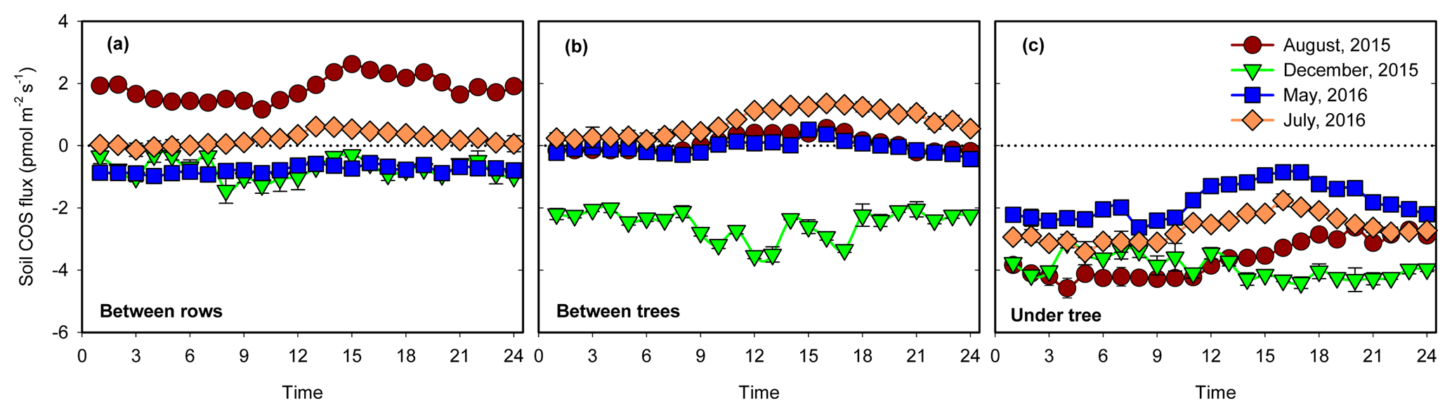
Figure 1 Spatial variability of soil COS flux at three sites: between trees (a), between rows (b) and under tree (c). Each panel shows the diurnal cycling of soil COS flux in the four campaigns. Each data point was the hourly mean ±1 SE (N=3).

On the diurnal timescale, soil COS flux were generally higher in the afternoon (peaking around 15:00–16:00), declining at night and in the early morning (Fig. 1). On the seasonal timescale, soil COS fluxes showed both changes in rates and shifts from net uptake to net emission, with the site hierarchy differing in the different seasons (Fig. 1). At the UT site where only COS uptake was observed, the highest rates were observed in winter and peak summer (December and August) with diurnal mean rates of nearly −4 pmol m⁻² s⁻¹ and more moderate uptake rates of around −2 pmol m⁻² s⁻¹ in spring and early summer (May and July; Fig. 1). At the BT sites, significant COS uptake of $\sim -\mathrm{2.5}$ pmol m⁻² s⁻¹ was observed in winter, but net fluxes were near zero at other times, with some afternoon emission in summer. At the exposed BR sites, minor uptake (less than −1 pmol m⁻² s⁻¹) was observed in spring and early summer, but there was consistent emission in peak summer, with diurnal mean values of nearly +2 pmol m⁻² s⁻¹.

3.2 Effects of moisture and temperature

During the hot summer (August 2015 and July 2016), differences in micro-site soil water content (θ) were most distinct, with θ of nearly 30 % at the UT sites (associated with drip irrigation) but of ∼19 % and ∼12 % at the BT and BR sites. Correspondingly, the UT sites had significant COS uptake of about −3 pmol m⁻² s⁻¹, while the other sites showed emission of about +1 pmol m⁻² s⁻¹ (Table 1). In winter (December), θ at the three sites was similar (∼25 %), and all sites showed soil COS uptake, but with clear gradients of −3.9, −2.5 and −0.7 pmol m⁻² s⁻¹ at the UT, BT and BR sites, respectively (Fig. 1). On average, soil COS fluxes showed a nonlinear increase in uptake with increasing θ, but it seems that this response may saturate at about θ of 25 % and uptake rates of $\sim -\mathrm{3.9}$ pmol m⁻² s⁻¹ (Fig. 2). The fit to the data presented in Fig. 2 also indicate that in dry soil with θ < 15 %, soil COS emission can be expected.

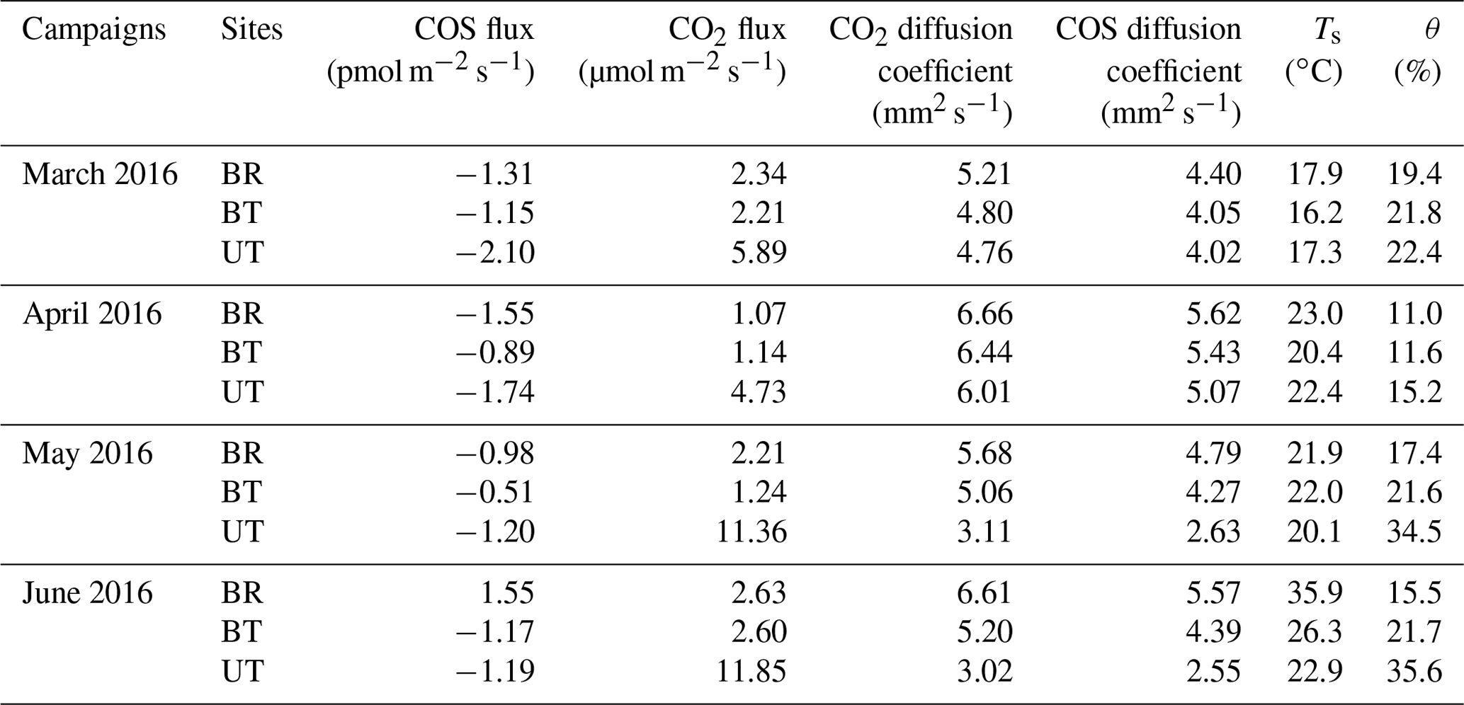
Table 1 Mean values of soil COS and CO₂ flux rates across sites (BR, between rows; BT, between trees; UT, under tree) and seasons, together with the normalized ratio of COS∕CO₂ fluxes (SRU), the mean soil temperature at 5 cm depth (T_s) and soil water content (%wt; θ).

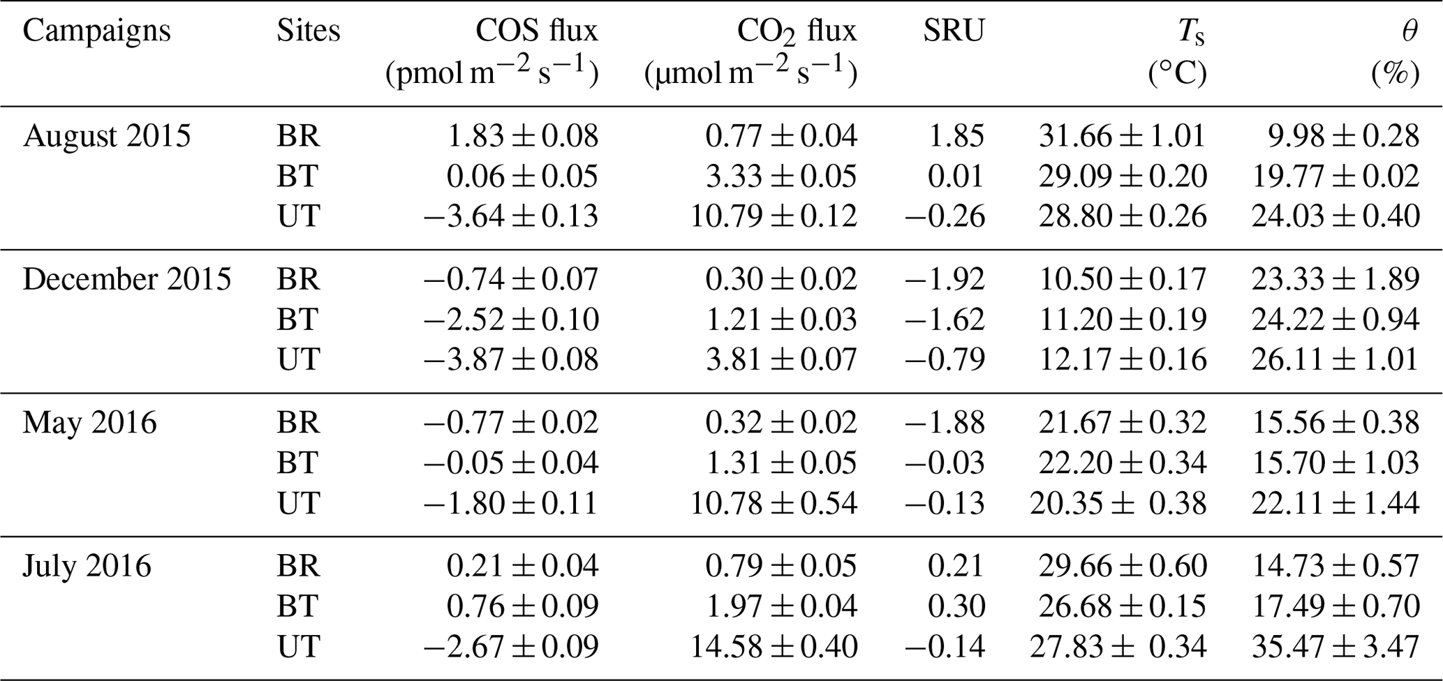
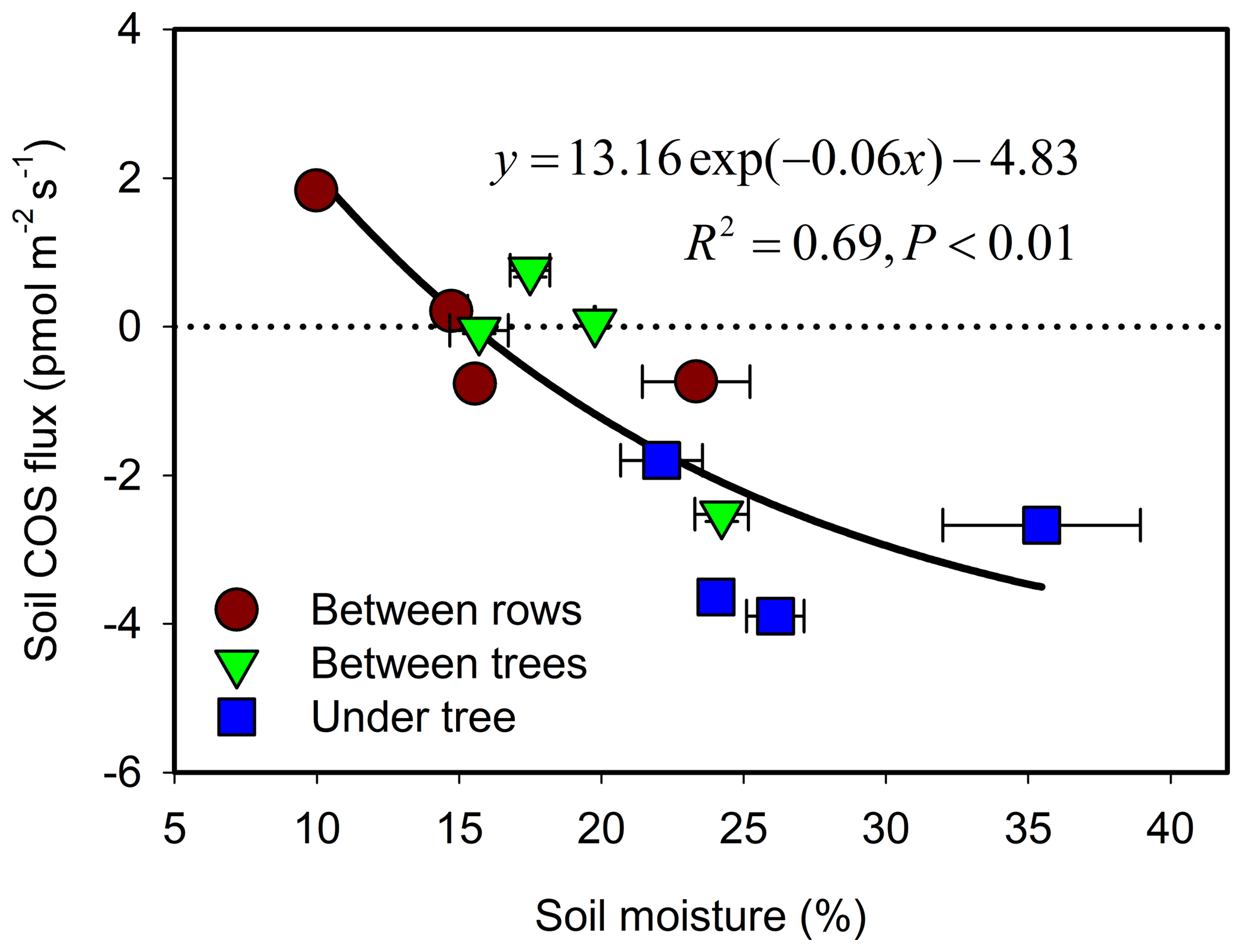
Figure 2 Relationship of soil COS flux and soil moisture. Each data point represents the diurnal average (N=24) for each micro-site and season (measurement campaign). Error bars represent ±1 SE around the mean; errors for flux are about the size of the symbols.

The response of soil COS fluxes to soil temperature varied among the three measurement sites (Fig. 3). The BT and BR sites showed a near-linear response with a shift from uptake to emission around 25 ^∘C. At the shaded and moist UT site, COS uptake was always significant, ranging between −4 and −1 pmol m⁻¹ s⁻¹ with relatively low temperature sensitivity, and with lowest mean uptake rates around 20 ^∘C.

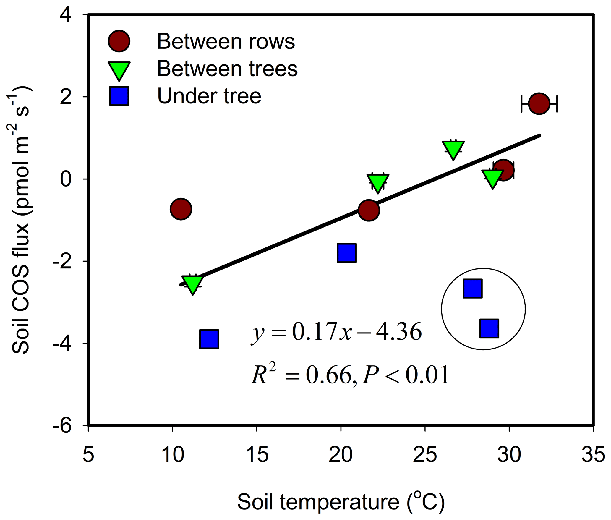
Figure 3 Soil COS flux as a function of temperature and its linear regression line. Each data point represents the diurnal average (N=24) for each site and season (campaign). Error bars ±1 SE around the mean. The data points marked by black circle were collected during irrigation cycle (enhanced uptake) and were excluded from the regression.

Pearson product–moment correlation analysis results showed that hourly soil COS flux was significantly related to soil moisture and temperature (at the 0.001 level), and the soil moisture had stronger environmental controls on the soil COS flux ($r=-$0.77) than soil temperature ($r=+$0.45).

A comprehensive assessment of the effects of soil moisture (θ), temperature (T_s) and distance from tree trunk (d) showed that hourly soil COS flux (F_COS) could be fitted to a three-parameter exponential model, which could explain 75 % of the variation in soil COS flux (Eq. 6).

$$\begin{array}{ll}{\displaystyle }{F}_{\mathrm{COS}}=& {\displaystyle }\mathrm{8.91}\exp (\mathrm{0.01}{T}_{\mathrm{s}}-\mathrm{0.01}\mathit{\theta }+\mathrm{0.09}d-\mathrm{0.33})-\mathrm{8.86}\\ \text{(6)}& {\displaystyle }& {\displaystyle }{R}^{\mathrm{2}}=\mathrm{0.75}\end{array}$$

3.3 COS flux estimates from soil concentration gradients

The average soil concentration gradient of COS and CO₂ for the four campaigns is shown in Fig. 4. COS concentrations decreased with soil depth, with the opposite trend for CO₂, consistent with the results reported above of soil surface COS uptake and CO₂ emission at our orchard site. COS concentrations at a depth of 2.5 cm were on average 314 ppt, about one-third lower than the mean surface ambient value of 460 ppt. The lowest COS concentration at a depth of 20 cm (166 ppt) was almost one-third of that at the soil surface. An exponential and a linear equation provided a reasonable fit to the changes in soil COS and CO₂ concentrations, respectively, as a function of depth (z_soil):

$$\begin{array}{ll}{\displaystyle }\left[\mathrm{COS}\right]=& {\displaystyle }\mathrm{283.5}\exp \left(-\mathrm{0.2}{z}_{\mathrm{soil}}\right)+\mathrm{169.9},R^{\mathrm{2}}=\mathrm{0.99},\\ \text{(7)}& {\displaystyle }& {\displaystyle }\left[{\mathrm{CO}}_{\mathrm{2}}\right]=\mathrm{122.2}{z}_{\mathrm{soil}}+\mathrm{558.5},R^{\mathrm{2}}=\mathrm{0.99}.\end{array}$$

In terms of individual sites and campaigns, all profiles except for BR in summer (June) showed the general trend of decreasing [COS] and increasing [CO₂] with depth, with the steepest gradient in the top 5 cm (Fig. 5). At the BR micro-site in summer, CO₂ profiles were shallow, consistent with low respiration (see July BR in Table 1). But a decrease in COS concentration toward the surface, with a surface value lower than the next two soil depth points (Fig. 5j), was consistent with COS emission at that time (July BR in Table 1).

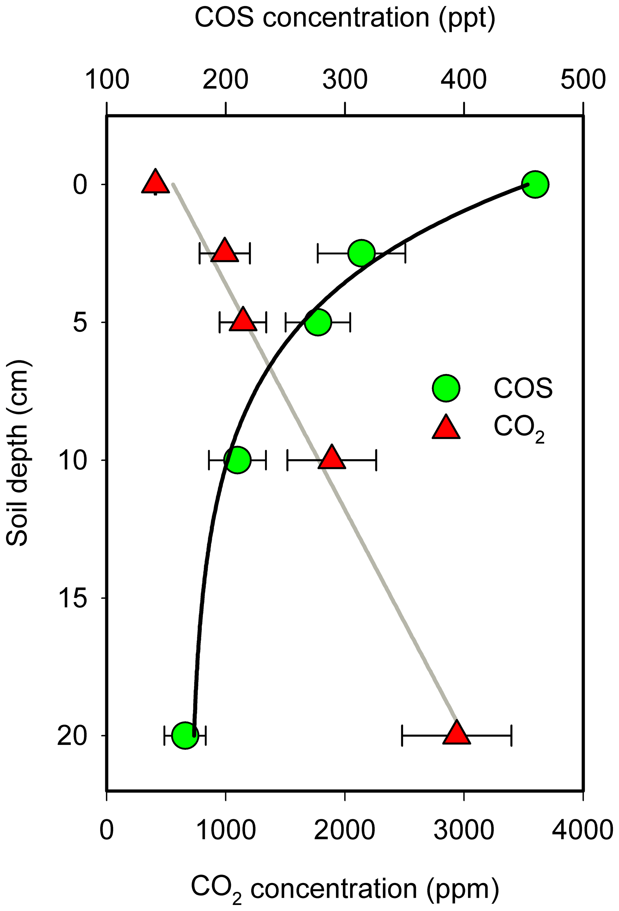
Figure 4 Mean COS and CO₂ concentrations at different soil depths. The COS concentration decreases exponentially with soil depth. The data point is the mean of the combined data at each of the four measurement campaigns (N=4; ±1 SE).

Figure 5 Soil COS and CO₂ concentration profiles at the three micro-sites in four measurement campaigns. The data points are the mean of all measurements in a campaign (N=4, ±1 SE).

As noted above, the profile data generally exhibited the steepest gradient in the top few centimeters of the soil, indicating that the dominating COS sink (and likely also the CO₂ source) was located at shallow depth. We therefore used the gas concentration difference at the two shallowest depths (z_soil1=0 and z_soil2=2.5 cm) to provide an approximation of the fluxes to and from the soil to constrain the more extensive chamber measurements. The COS diffusion coefficient, D_s, was estimated for each campaign (see “Materials and methods”), indicating a low D_s value at the UT site in June and July (D_s=2.55 mm² s⁻¹) associated with the drip irrigation and the high soil water content and high values in the dryer soils (D_s=5.57 mm² s⁻¹), with an average COS diffusion coefficient of 4.4±0.3 mm² s⁻¹. The soil COS flux estimates using the gradient method are reported in Table 2. COS flux varied between −2.1 and +1.6 pmol m⁻² s⁻¹ with a mean value of $-\mathrm{1.0}\pm \mathrm{0.3}$ pmol m⁻² s⁻¹ during the measurement periods, consistent with the mean value of 1.1±0.1 pmol m⁻² s⁻¹ reported above for the chamber measurements. Also in agreement with the chamber measurements, fluxes at UT and BT always showed COS uptake, with generally higher values in spring (March) than in summer (May–June), while the BR data indicated change from uptake in spring (March–April, −1.3 to −1.6 pmol m⁻² s⁻¹) to emission in June (+1.6 pmol m⁻² s⁻¹).

Table 2 Estimates of soil COS and CO₂ fluxes from soil concentration gradient measurements (T_s, soil temperature; θ, soil water content; BR, between rows; BT, between trees; UT, under tree).

3.4 Soil relative uptake

Soil was always a source of CO₂ due to respiration (combined autotrophic and heterotrophic respiration). Soil CO₂ flux rates varied both spatially and temporally in similar patterns to those of COS and with an overall range of +0.3 to +14.6 µmol m⁻² s⁻¹ (Table 1). The highest soil respiration values were observed at the UT sites in summer (July, August; Table 1), with intermediate (+1 to about +3 µmol m⁻² s⁻¹) and low values (<+1 µmol m⁻² s⁻¹) at the BT and BR sites, respectively. Generally, soil COS exchange varied from release to increasing uptake with increasing CO₂ production in a nonlinear way (Fig. 6a). The normalized ratio of COS to CO₂ fluxes (SRU; Eq. 2) varied from −1.9 to +1.9, with an average value of $-\mathrm{0.4}\pm \mathrm{0.3}$, with negative values indicating COS uptake linked to CO₂ emission. SRU values showed a response to both soil temperature (Fig. 6b) and soil moisture (Fig. 6c), although with relatively low R² values. Respiration increased with temperature while COS uptake declined, and at temperatures above about 25 ^∘C, SRU turned positive when both COS and CO₂ were emitted from the soil. SRU exhibited inverse relationships with soil moisture, with positive values in dry soil and increasingly negative values with increasing soil moisture (Fig. 6c). Based on its combined temperature (T_s) and moisture (θ) response, SRU could be forecasted by the following algorithm, which explained 67 % of the observed variations (Eq. 8):

$$\begin{array}{}\text{(8)}& {\displaystyle }\mathrm{SRU}=\mathrm{0.01}\exp \left(\mathrm{0.17}{T}_{\mathrm{s}}\right)-\mathrm{0.02}\mathit{\theta }-\mathrm{1.00},R^{\mathrm{2}}=\mathrm{0.67}.\end{array}$$

ANOVA results indicated that SRU was not significantly different among the three observation micro-sites (BR, BT and UT; P > 0.05). Between the seasonal campaigns, however, SRU values peaked in summer ($+\mathrm{0.5}\pm \mathrm{0.7}$), with the highest averaged soil temperature (29 ^∘C), and were significantly higher than winter SRU ($-\mathrm{1.4}\pm \mathrm{0.6}$) when soil temperature was lowest (11 ^∘C; P < 0.05). There was no significant difference in SRU among the other campaigns (P > 0.05).

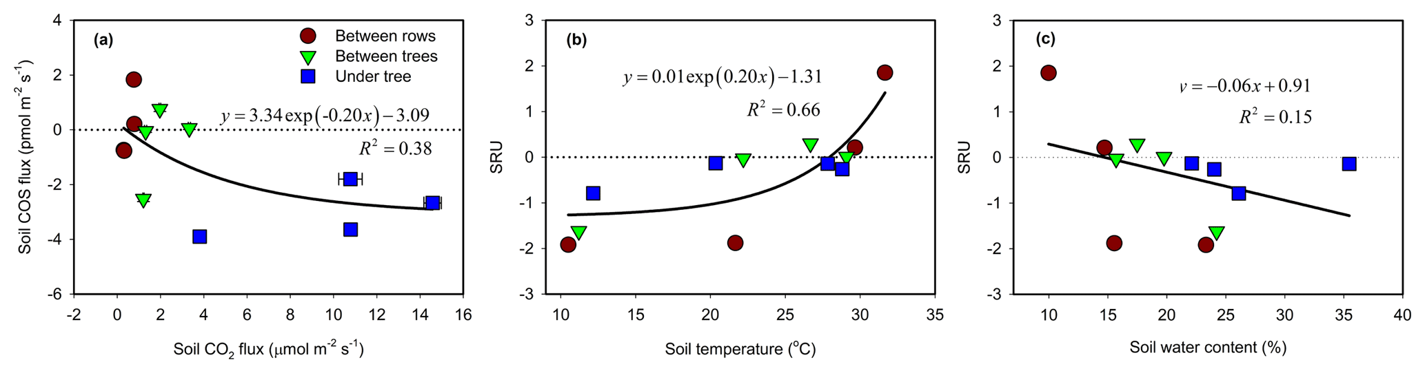
Figure 6 The relationships between soil COS and CO₂ flux rates (chamber measurements a). The response of soil relative uptake (SRU; normalized ratio of COS to CO₂ fluxes) to soil temperature (b) and to soil water content (c). The data points represent the diurnal average (N=24) of each site and season (measurement campaign). Error bars represent ±1 SE around the mean (often the size of the symbol).

4 Discussions

4.1 Heterogeneity in soil COS exchange

The observed soil–atmosphere COS exchange rates observed in this study (both mean and range; Fig. 1, Table 1) are consistent with values reported in a range of other ecosystems (−1.4 to −4.9 pmol m⁻² s⁻¹; Steinbacher et al., 2004; Kitz et al., 2017; White et al., 2010; Berkelhammer et al., 2014) but lower than −11.0 to −11.8 pmol m⁻² s⁻¹ in riparian and subtropical forests (Berkelhammer et al., 2014; Yi et al., 2007). Soil COS emissions were also observed in the summer and spring campaigns, with maximal COS emission consistent with the values of +1.8 to +2.6 pmol m⁻² s⁻¹ observed in riparian and alpine forests (Berkelhammer et al., 2014) but significantly lower than reported in the senescing agricultural ecosystem ($\sim +\mathrm{30}$ pmol m⁻² s⁻¹; Maseyk et al., 2014).

The observed range in the soil–atmosphere exchange fluxes reflected significant heterogeneity on both the spatial and the temporal scales. The spatial-scale heterogeneity clearly reflected the contrasting micro-site conditions with lower temperatures and higher moisture under the trees (UT sites) compared with the higher temperatures and lower moisture in exposed soil between rows (BR sites), with intermediate, partially shaded, conditions between trees (BT sites). Indeed, a large fraction of the variations in the COS flux (∼75 %) could be explained by a simple algorithm as a function of these two variables: temperature and moisture. Note that while temperature and θ covaried in general, with high temperatures associated with drier soil, under the wet UT conditions, sensitivity to temperature was significantly reduced. In the dry soil conditions, emission was associated with high temperature and at the BR sites also with high solar radiation. However, all measurements were made in dark chambers and could not involve photochemical production, which was also demonstrated in agricultural soil by Kitz et al. (2017). Apparently even under dark conditions, high temperature can induce high emission rates, as also noted when the thermal insolation on the soil chamber at the BR site was occasionally removed and a large spike in temperature (52 ^∘C) and emission of 11.4 pmol m⁻² s⁻¹ was observed. Note also that the soil profile results indicated that the emission source was below the surface and maybe non-photochemical irrespective of the chamber opaqueness.

Temporal variations were observed both on the daily and seasonal timescales. Diurnal changes were, however, minor compared to the changes from winter to summer at all micro-sites. Shifts from uptake to emission were observed essentially only on the seasonal timescale (Fig. 1). This likely reflected the dominance of soil moisture in relation to the COS flux rates. This is because θ did not change noticeably on the daily scale, while it did changed considerably across seasons (between 10.0 and 35.5 % overall). Soil temperatures did change over the daily cycle (e.g., 26.0 to 42.4 ^∘C at the BR site during summer), although such changes are still smaller than the seasonal changes in soil temperature (e.g., 10.5 to 31.8 ^∘C at the BR site). A dominant role of soil moisture in explaining the variations in COS uptake is consistent with the results of Van Diest and Kesselmeier (2008) but less so with the negligible θ effects in grassland under simulated drought (Kitz et al., 2017).

COS uptake is thought to be related to carbonic anhydrase (CA) activity in soil (Kesselmeier et al., 1999), which could be via microorganisms (Piazzetta et al., 2015), such as bacteria (Kamezaki et al., 2016; Kato et al., 2008) or fungi (Bunk et al., 2017; Li et al., 2010; Masaki et al., 2016). CA activity is also influenced by soil moisture (Davidson and Janssens, 2006; Seibt et al., 2006), although soil moisture can also directly influence soil gas diffusion rates (Ogée et al., 2016; Sun et al., 2015). The effect of CA on COS exchange can also be related to root distribution and the effects of CA activity within plant roots (Seibt et al., 2006; Viktor and Cramer, 2005; Whelan and Rhew, 2015). This could influence the spatial variations and soil moisture effects on COS exchange in this study as most of the roots were distributed around the restricted trees' drip irrigation zone at UT sites and were sparse in the dryer areas, such as the BR and BT sites (unquantified observations).

At least part of the variations in soil COS fluxes could also reflect the differential effects of environmental conditions on COS uptake and production process (Ogée et al., 2016). Solubility in soil water (with a COS solubility of 0.8 mL mL⁻¹; Svoronos and Bruno, 2002) could also be significant, especially at the UT micro-sites, influenced by the drip irrigation from May to September, which could involve water percolation to deeper soil layers. The drivers of soil COS production are still unclear. COS could be produced by chemical processes in the lab (Ferm, 1957) but can also be produced by biotic process in soils such as hydrolysis of metallic thiocyanates (Katayama et al., 1992) with thiocyanate hydrolase (Conrad, 1996; Svoronos and Bruno, 2002) and hydrolysis of CS₂ (Cox et al., 2013; Smith and Kelly, 1988). Fungi are also reported to be the source of COS (Masaki et al., 2016). Additionally, abiotic thermal degradation of organic matter leading to COS production may be consistent with the temperature sensitivity of COS emission at the BR micro-site where biotic processes can be expected to be minimized. Similar high temperature-dependent soil COS emissions were reported in midlatitude forests (Commane et al., 2015) and an agricultural field (Maseyk et al., 2014). Lab incubation results also indicated thermal production of COS in soil with increasing temperature (Liu et al., 2010; Whelan et al., 2016; Whelan and Rhew, 2015). Photochemical production of soil COS was also proposed (Sun et al., 2015; Whelan and Rhew, 2015), and assumed to be driven by ultraviolet fraction of incoming solar radiation (Kitz et al., 2017). Note, however, that all measurements in the present study were made in the dark. In addition, the chemical reaction of CO and MgSO₄ under heating could also produce COS (Ferm, 1957). Note that MgSO₄ has been reported in our study soil (Singer, 2007), and we observed a relatively high CO concentration at our field site (not shown due to insufficient calibration). Finally, the balance between the uptake (likely biotically dominated) and emission (likely abiotically dominated) can also be influenced by soil nitrogen (Kaisermann et al., 2018).

4.2 Soil relative uptake

We use SRU values to assess the relative importance of the soil COS flux compared with the canopy and indicate shifts from conservative links between processes influencing COS and CO₂ (see the Introduction). On average, the value of SRU at our site was smaller than reported for riparian or pine forests (−0.37 vs. −0.76 and −1.08; Berkelhammer et al., 2014; Sun et al., 2018). This may reflect the contribution of COS emissions at BR and BT in summer that were not observed in the forest study. Overall, the mean SRU values observed here indicated that the soil COS uptake flux was proportionally less than 40 % of the soil respiration flux. In contrast with the canopy fluxes where the COS uptake flux is proportionally nearly twice as large as the CO₂ assimilation flux (LRU ∼1.6 at our site; Yang et al., 2018; 1.7 across vegetation types, Whelan et al., 2018). In contrast to leaves with robust LRU values that tend toward a constant, SRU at our site varied between −1.9 and +1.9. However, this range was observed only at the dryer and exposed BR sites, while in the shaded and moist UT sites, it was much narrower: −0.1 to −0.8. Furthermore, it seems that the high SRU values (both positive and negative) represented conditions where the actual fluxes were small (COS uptake was on average −3.0 in the UT but only 0.1 pmol m⁻² s⁻¹ at the BR sites). It seems that the large SRU values at the BR micro-sites were also associated with low soil respiration: 0.5 µmol m⁻² s⁻¹ at BR sites compared to 10 µmol m⁻² s⁻¹ at the UT sites. It is therefore possible that the low SRU values are more significant for ecosystem-scale studies and indicate a much smaller contribution to overall ecosystem fluxes than those of the canopy (i.e., $\mathrm{SRU}\sim -\mathrm{0.4}$ vs. $\mathrm{LRU}\sim +\mathrm{1.7}$).

The differential effects of changing environmental conditions on production and uptake processes were reflected in the relatively large spatial and temporal heterogeneity observed in the soil COS exchange at our site. However, the contrasting effects of production and emission may explain both the sharp increase in SRU values at high temperatures, as the effects of production counteract uptake (Fig. 6b), and the much lower sensitivity to temperature of COS flux compared to that of CO₂ (Fig. 6a). Such contrasting consumption or production effects may, in fact, reduce the magnitude of the net flux of soil COS and may explain the relatively narrow range of SRU values.

The application of COS as a tracer for canopy CO₂ exchange requires accounting for the soil effects, and while knowledge of SRU can help predict it, ultimately we need to quantify the fluxes. Note in that respect that in our recent canopy-scale study at the same site, Yang et al. (2018) indicated that in spite of the considerable variations in soil COS fluxes, the soil COS uptake fluxes were equivalent to ∼1 % of the daytime foliage flux across seasons and reached ∼3 % in the spring peak season (but larger proportions were observed during more stressful periods when fluxes were overall small).

4.3 Soil COS profiles

Complementing our chamber measurements with soil profile measurements of COS and CO₂ concentrations provided constraints on the relatively new surface soil COS measurements and provided additional information on the possible location of the source or sink in the soil. Using the near-surface gradient yielded flux estimates comparable to chamber measurements, providing a useful and rare quantitative validation. For example, in May, the chamber and profile measurements were made at about the same time (5–9 May for chamber and 10 May for profile), and the differences between chamber (all micro-sites) and gradient flux estimates was negligible (∼0.2–0.6 pmol m⁻² s⁻¹). However, the profile results also indicated that the sink or source activities were concentrated in the top soil layers, probably at around 5–10 cm depth, as reflected in the minimum or maximum in gas concentrations (emphasizing the need for a high vertical resolution in employing the profile approach). The variable profiles observed below these points must reflect temporal dynamics in the sink or source activities across the profile. The near-surface peak activity makes it particularly sensitive to variations in temperature and moisture, as observed (Figs. 2 and 3). Low COS concentration in the lower parts of the profile may result from the continuous removal of soil COS and may indicate a distribution of CA activity beyond the litter layer and the soil surface (Seibt et al., 2006). COS production, however, seems to occur only near the soil surface with no indication for production in deeper layers, consistent with its high temperature sensitivity and not necessarily dependent on radiation (e.g., Kitz et al., 2017).

Note that the gradient method based on the Fick's diffusion law has its own limitations (Kowalski and Sánchezcañete, 2010; Sánchez-Cañete et al., 2017; Bekele et al., 2007). However, it is a simple, low-cost approach and can help diagnose the magnitude of soil fluxes, which can also help in identifying belowground processes and their locations.

5 Conclusions

Our detailed analysis of the spatial and temporal variations in soil–atmosphere exchange of COS provided new information on a key uncertainty in the application of ecosystem COS flux to assess productivity. Furthermore, we provide validation of the surface chamber measurements that are generally in use, by the additional gradient approach. Our results show that both micro-sites and seasonal variations in COS fluxes were related to soil moisture, temperature and the distance from the tree (likely reflecting root distribution), but we suggest that soil moisture is the predominant environmental control over soil COS exchanges at our site. A simple algorithm was sufficient to forecast most of the variations in soil COS flux, supporting its incorporated into ecosystem-scale applications, as we recently demonstrated in a parallel study at the same site (Yang et al., 2018).

Clearly, uncertainties are still associated with soil processes involving COS, the differential effects of soil moisture, temperature and communities of microorganisms, and they are likely to contribute to both the spatial and temporal variations in soil net COS exchange and require further research.