Characterizing wind gusts in complex terrain

Wind gusts are a key driver of aerodynamic loading, especially for tall structures such a bridges and wind turbines. However, gust characteristics in complex terrain are not well understood and common approximations used to describe wind gust behavior may not be appropriate at heights relevant to wind turbines and other structures. Data collected in the Perdigão experiment are analyzed herein to provide a foundation for improved wind gust characterization and process-level understanding of flow intermittency in complex terrain. High-resolution observations from sonic anemometers and vertically pointing Doppler lidars are used to conduct a detailed study of gust characteristics with a specific focus on the parent distributions of nine gust parameters (that describe velocity, time, and length scales), their joint distributions, height variation, and coherence in the vertical and horizontal planes. Best-fit distributional forms for varying gust properties show good agreement with those from previous experiments in moderately complex terrain but generate nonconservative estimates of the gust properties that are of key importance to structural loading. Probability distributions of gust magnitude derived from vertically pointing Doppler lidars exhibit good agreement with estimates from sonic anemometers despite differences arising from volumetric averaging and the terrain complexity. Wind speed coherence functions during gusty periods (which are important to structural wind loading) are similar to less complex sites for small vertical displacements (10 to 40 m), but do not exhibit an exponential form for larger horizontal displacements (800 to 1500 m).

1 Introduction and objectives

Topographic channeling or enhancement of the near-surface flow can lead to local increases in wind speed (Wagenbrenner et al., 2016) and hence enhance the wind resource (Clifton et al., 2014; Barthelmie et al., 2016; Jubayer and Hangan, 2018). Terrain inhomogeneity also induces complex flow conditions (Wood, 2000), particularly in the presence of vegetation (Suomi et al., 2013), that have implications for wind loading on structures, pollutant dispersion, wildfire propagation, and wind turbine siting and operation (Sanz Rodrigo et al., 2017; Wagenbrenner et al., 2016; Butler et al., 2015). Key features of flow in complex terrain include thermo-topographic flows arising from differential heating (Rucker et al., 2008; Rotach and Zardi, 2007) and lee-side vortices that develop parallel to mountain ridges (Grubišić et al., 2008). Regions with complex topography and land cover heterogeneity also tend to experience more frequent and stronger wind gusts (herein defined as coherent short-term wind speed maxima) (Letson et al., 2018; Earl et al., 2017; Sheridan, 2011; Hasager et al., 2003) due in part to

1. terrain-induced alteration of the structure of mesoscale convective systems and thus the downdrafts and wind gusts generated therefrom (Markowski and Dotzek, 2011).

2. generation of small-amplitude mountain waves in stably stratified air that can cause strong and gusty downslope winds when the flow becomes supercritical and these waves “break” (see detailed discussion in Durran, 1990, and Hertenstein and Kuettner, 2005).

Wind gusts represent an important source of structural engineering loads for tall buildings, towers, bridges, and wind turbines (Solari, 1987; IEC, 2005; Cheynet et al., 2016), and are known to be of larger magnitude in complex terrain due in part to the factors listed above (Tieleman, 1992; Verheij et al., 1992). A number of numerical wind flow models have been developed for application at high spatial resolution over complex terrain, but model evaluation has been severely constrained by the lack of suitable observational data (Butler et al., 2015; Bechmann et al., 2011; Berg et al., 2011; Suomi and Vihma, 2018). Further, most past research on flow intermittency has focused on the intensity (i.e., magnitude) of wind gusts and has employed measurements from 10 m a.g.l. (e.g., Vickery and Skerlj, 2005). Thus, there is a need to advance understanding of the spatiotemporal coherence of wind gusts at heights above 10 m a.g.l., in complex terrain (Belu and Koracin, 2013; Mouzakis et al., 1999), and for better characterization of both (i) the height variation in gust properties (Suomi et al., 2013) and (ii) additional descriptors of wind gusts such as gust rise times and length scales since these properties also contribute to the wind-excited structural response (Solari, 2014; Frost and Turner, 1982) and fatigue loading on wind turbines (Chamorro et al., 2015; Hu et al., 2016). The gust parameters and probability distributions used herein to describe the behavior of wind gusts in complex terrain are designed to mirror those used in Hu et al. (2018), so that clear comparisons can be made between the results of the current study and those derived from measurements in less complex terrain.

Herein we address these research needs using data collected during January–July 2017 at a site in eastern Portugal near Perdigão (Fig. 1a). Two parallel ridges running from the northwest to southeast and separated by 1.4 km dominate the local topography in the study area. These ridges stand 300 to 350 m above the surrounding terrain and approximately 175 m above the valley located between them (Fig. 1b). This location was the focus of a measurement campaign during which over 50 meteorological masts were deployed over an area of a few square kilometers (Mann et al., 2017). The data collected in the Perdigão experiment and employed herein to characterize flow behavior at heights relevant to wind turbine selection, operation, and micro-siting with a specific focus on wind gusts are high-frequency (18 Hz) 3-D wind measurements from Gill WindMaster Pro sonic anemometers deployed on the nine tallest of the meteorological masts (that extended to heights (z) above 50 m a.g.l.) and horizontal wind speeds from two vertically pointing conically scanning (ZephIR) Doppler lidars (locations of these instruments are shown in Fig. 1b and Table 1; details of the measurement technologies are given in Sect. 2).

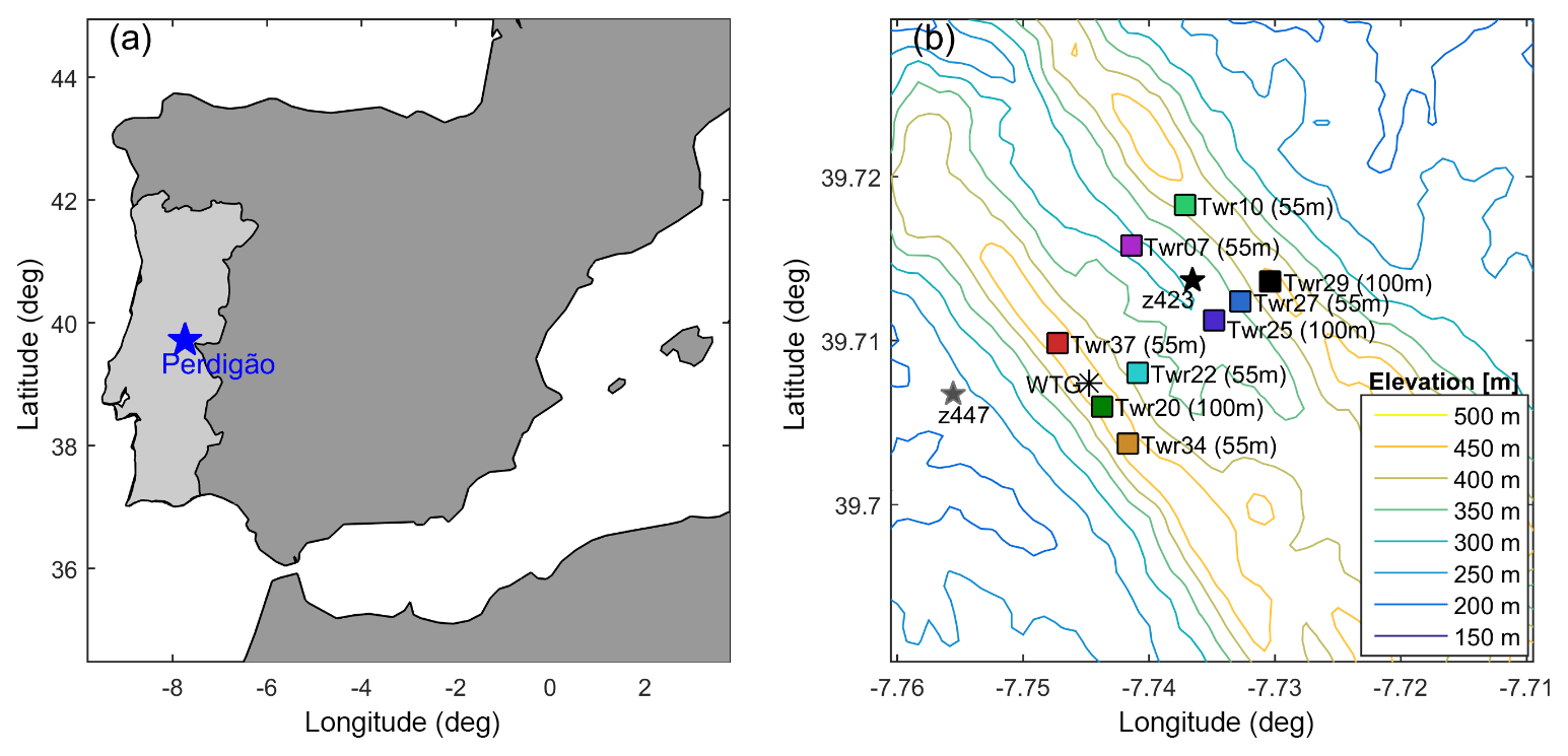
Figure 1 (a) Location of the Perdigão measurement site in Portugal. (b) Overview of the tower and ZephIR lidar locations and site topography (measured by the Shuttle Radar Topography Mission; Farr et al., 2007). The height of each tower is shown in parentheses. The nine colors shown in this figure are used to distinguish the nine towers throughout the paper. A single wind turbine is located on the SW ridge (denoted by WTG^∗).

The objectives of the current study are as follows.

• Evaluate the degree to which the best-fit probability distributions to various gust parameters (e.g., intensity, temporal scale, and length scale) as advanced by Hu et al. (2018) are generalizable across terrain types. The resulting parametric descriptions of gust properties are potentially of utility to the engineering community because they permit estimation of extreme values (IEC, 2005; ASCE, 1998) (e.g., using Rice theory; Gomes and Vickery, 1977), facilitate development of joint distributions of gust parameters, allow characterization of gusts that contribute to structural fatigue, and are used with design standards (for example, extreme gusts are modeled in wind turbine design standards based on mean wind speeds and turbulence intensity; IEC, 2005). They are potentially also of use within the meteorological community since they could afford a methodology for downscaling of wind gusts in either weather forecasting (Friederichs and Thorarinsdottir, 2012; Suomi and Vihma, 2018) or climate downscaling contexts (Cheng et al., 2014). Further, fluctuating wind loads on engineering structures requires estimates of multiple components of the flow, including characteristics that have previously received relatively little attention (e.g., the shape of wind gusts) (Mücke et al., 2011; Suomi et al., 2013). Various parametric distributions are evaluated in terms of their goodness of fit to the empirical data and their accuracy at the distribution tails and are used to develop joint probability distributions of different gust properties at a single location and of the same gust property across space (where the latter can be used to develop bivariate extreme value copulas; Bonazzi et al., 2012). Where possible the distributional forms for each gust parameter are compared with previous work in flat or moderately complex terrain (Morgan et al., 2011; Cheng and Bierbooms, 2001; Friederichs and Thorarinsdottir, 2012; Hu et al., 2018).

• Quantify the dependence of different descriptors of wind gusts on measurement height (z). Data from comparatively flat terrain show evidence that the characteristics of wind gusts, and particularly gust factors (GFs) and gust durations, vary systematically with height (Román, 2017; Suomi et al., 2015, 2013; Ashcroft, 1994). We seek to describe the magnitude and nature of this variability with height in complex terrain by conditionally sampling gust properties as derived from the sonic anemometers deployed on the meteorological masts and as determined from vertically pointing ZephIR lidars.

• Characterize power spectra of wind speeds from sonic anemometers and ZephIR lidars at different heights. These power spectra are used to determine how the presence of wind gusts affects their shape (Hu et al., 2018) and to derive first-order estimates of the so-called reverse height (i.e., height above ground at which surface-driven processes cease to dominate scales of variability) using the amount of variance expressed at the diurnal timescale (Larsén et al., 2018; Troen and Lundtang Petersen, 1989). In the near-surface levels surface-driven processes produce the diurnal peak in the power spectrum of wind speeds, while aloft it is primarily the product of pressure perturbations deriving from the atmospheric tide (Larsén et al., 2018). At intermediate heights there is a relative minimum in the amount of variance expressed at periods ≈ 1 day. At these heights the first-order effect of the surface heat-flux modulations vanishes (Larsén et al., 2018), and thus it may provide an estimate of the height at which surface-driven processes cease to dominate scales of variability.

• Quantify the dependence of wind gust parameters on atmospheric conditions; specifically stability, wind direction, and turbulence intensity (Barthelmie et al., 2016; Hu et al., 2018). Previous work has shown that GFs are strongly and directly related to turbulence intensities (Ashcroft, 1994; Greenway, 1979; Hu et al., 2018) and that turbulent kinetic energy (and hence the potential for gusts) is enhanced downstream of obstacles (Jubayer and Hangan, 2018). Thus, wind gust properties at the nine towers are conditionally sampled by wind direction, stability class, and by turbulence intensity.

• Quantify spatial coherence in flow properties, particularly wind gusts. The physical scales of wind gusts are critically important to loading on structures (Solari, 1987; Hui et al., 2009; Bos et al., 2016), and the potential for gusts to remain coherent as they propagate through a wind farm has implications for power quality and grid management (Sørensen et al., 2002; Vigueras-Rodríguez et al., 2012). The frequency characteristics of longitudinal wind speed are investigated using spectral analysis of output from individual sonic anemometers and coherence functions among pairs of sonic anemometers during gusty periods. Horizontal coherence functions between sonic anemometers on different masts and thus displaced by distance of hundreds of meters are used to describe the degree to which wind gust variations are coherent in the complex terrain of the study area, and comparisons are made to coherences from previous work.

2 Data

2.1 Sonic anemometer observations

The primary data set analyzed herein comprises 18 Hz, wind components, and sonic virtual temperature as measured by Gill WindMaster Pro sonic anemometers deployed on these meteorological masts (Table 1 and Fig. 1) at heights above the surrounding vegetation. The three tallest towers have seven measurement heights (z) each extending from 10 to 100 m a.g.l. and the remaining six towers have five measurement heights each extending from 10 to 55 m. The 18 Hz signals from each sonic anemometer are subject to coordinate rotation (including corrections for the boom alignment) and despiking using a 5σ filter in each 10 min period. In order to ensure that our characterization of spatial variations in wind gust parameters is not biased by differing measurement periods, the current analyses are restricted to days that have complete data records at all anemometers. Data analyzed here represent all 24 h periods during which all of the 41 sonic anemometers had >90 % of all 18 Hz signals present in >99 % of the 10 min periods (143 out of 144 10 min periods in each day). Analyses of gust parameters based on data from the ZephIR Doppler lidar measurements are also for the same 64 24 h periods.

Table 1 Locations and measurement heights of each meteorological mast (tower) and each ZephIR lidar. Measurement heights referred to in this paper as “60 m” are shown in bold. Reference tower (Tower 29) is emphasized by italics. Tower base elevations are given in meters above sea level (a.s.l.) and mean vegetation height is calculated from aerial laser scans in a 50 m square cell surrounding each tower or ZephIR lidar. Definitions used to conditionally sample the towers as valley or ridge are also shown along with a parenthetical statement of their location on the northeast (NE) or southwest (SW) ridge. Valley towers are those with elevations below 400 m a.s.l.

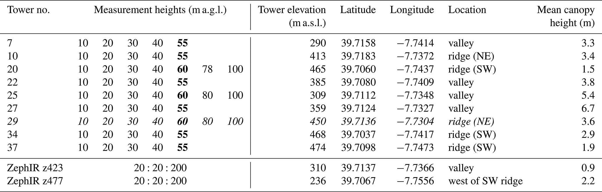
Tower 29, the 100 m tower on the northeast ridge (Fig. 1), is used herein as a reference tower to represent pseudo free-stream flow and characterize the prevailing atmospheric stability because of the prevalence of northeasterly flow during the field experiment (Fig. 2). Measurements from this meteorological mast indicate a high frequency of flow perpendicular to the ridges. Wind directions between 30 and 60^∘ occurred during 20 % of the 10 min periods while wind directions between 210 and 240^∘ occurred during 14 % of the 10 min periods (Fig. 2c). At Tower 29, the mean 10 min wind speed at 60 m is 5.0 m s⁻¹, and the mean turbulence intensity for mean wind speeds >3 m s⁻¹ is 0.14 (Fig. 2a, c). The greatest height represented at all nine meteorological masts is 55 or 60 m. Thus, this height is used to compare wind conditions across the study domain and is referred to herein as the 60 m measurement height for brevity. In some of the following analyses the meteorological masts (towers) are classified as “ridge” or “valley”, for which the former group have base elevations above 400 m a.s.l., and the latter are at elevations below that level (see Table 1).

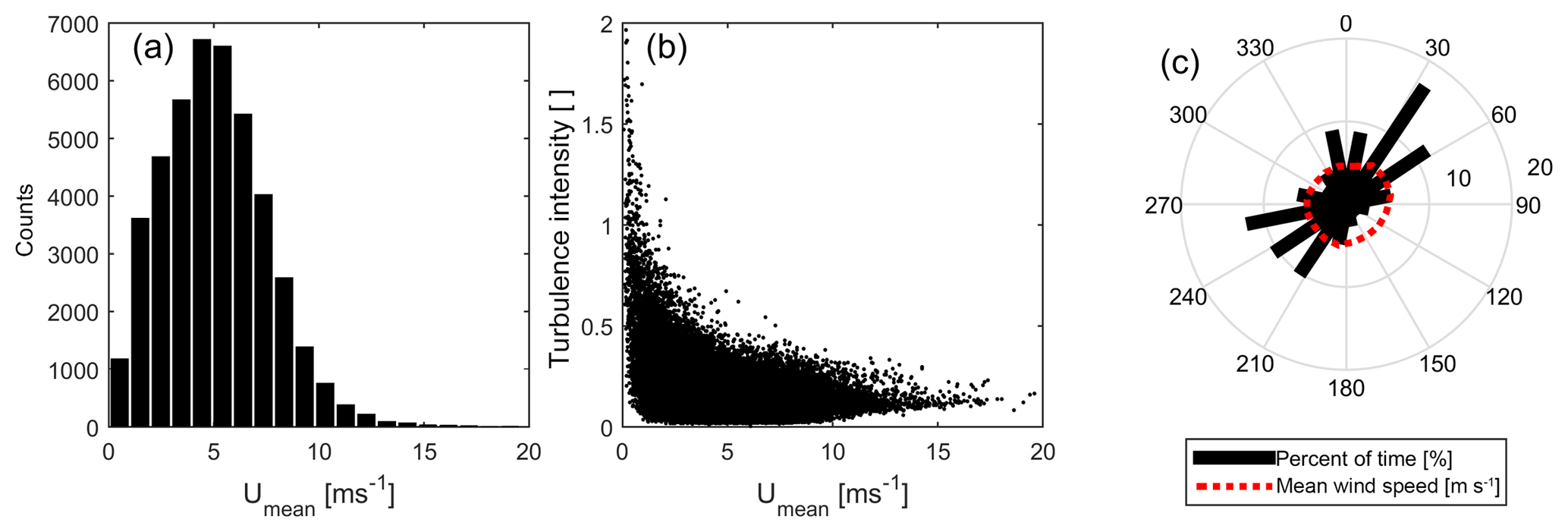
Figure 2 Overview of wind conditions at Perdigão. (a) The 10 min mean wind speed distribution at 60 m a.g.l. on Tower 29. (b) The 10 min turbulence intensities versus mean wind speed at 60 m a.g.l. on Tower 29. (c) Wind rose (black bars) and mean wind speed (red dotted line) from data collected at 60 m a.g.l. on Tower 29.

2.2 Doppler lidar observations

Lidars used in atmospheric applications can employ either light emitted in continuous-wave or pulsed forms (Held and Mann, 2018; Vasiljević et al., 2017). Measurements from two ZephIR continuous-wave Doppler lidars (referred to here as “lidars” and by their unit numbers, z447 and z423) are used to extend the analysis of gust parameters to heights above 100 m a.g.l. One ZephIR lidar was deployed in the central valley 311 m from meteorological mast 25 and one to the west of the SW ridge (Fig. 1b; locations in Table 1). The ZephIR 300 series is a continuous-wave coherent monostatic lidar that has a wavelength of 1.575 µm and an operating frequency of 50 Hz (Smith et al., 2006). It is vertically pointing (i.e., conducts velocity azimuth display scans) using a rotating prism to direct the laser over a scanning cone angle of 30^∘, and it measures the Doppler shift for 50 data points every second across a full 360^∘ scan (i.e., separation in the azimuth is approx. 7^∘). This variation in azimuth scan angle is necessary to convert from the Doppler shift derived from motion along the line of sight to the horizontal wind speed, and several hundreds of Doppler spectra are averaged in each azimuth sector. For all continuous-wave lidars there is an ambiguity in the identification of the dominant frequency in the Doppler spectrum so a range of methods have been developed to derive that frequency, and in the case of the ZephIR 300 it is identified from the centroid of the power spectral density above a noise threshold (Held and Mann, 2018). The Rayleigh length (a measure of the probe volume) scales with the square of the focus distance from the lidar. For the ZephIR 300 the probe length is 0.07 m at 10 m and 7.7 m at 100 m. These instruments were configured to measure horizontal wind speeds at 10 measurement heights (20 to 200 m a.g.l. at 20 m intervals), sampling at each height once every 17 s. Conically scanning Doppler lidars have been subject to extensive field validation (Gottschall et al., 2012). However, these Doppler lidars assume the flow to be homogeneous across the scanning volume in order to infer the horizontal wind speed. The radius (and circumference) of the annulus for the ZephIR 300 at a height of 100 m is thus 58 m (363 m) and at 200 m it is 115 m (726 m). Hence this assumption of homogeneity across the scanned annulus is not fulfilled in complex terrain, leading to increased uncertainty and potentially error in retrieved horizontal wind speeds (Bingöl et al., 2009). Further, the volumetric averaging inherent in the use of lidars means the wind speeds are not directly equivalent to those from in situ anemometry. Nevertheless, vertically pointing Doppler lidars offer the potential to quantify wind gusts at heights above those possible from sonic anemometers deployed on meteorological masts (Suomi et al., 2017) and are increasingly being adopted by the wind energy research and operations communities (IEA Wind Task 32 lidar for wind energy deployment) (Clifton et al., 2018). Herein, we evaluate the degree to which the probability distribution of gust amplitudes and GFs derived from the maximum of the disjunct measurements sampled at each of 10 heights (effective duration of ≈ 2 s) in each 10 min period correspond to those from the 18 Hz data from the sonic anemometers. We also use time series of 10 min mean wind speeds from each height (up to 200 m a.g.l.) from the ZephIR lidars to investigate the reverse height (implied by the magnitude of the diurnal peak, estimated across the frequency range; $\mathrm{3}\times {\mathrm{10}}^{-\mathrm{6}}$ to $\mathrm{2}\times {\mathrm{10}}^{-\mathrm{5}}$ Hz) and to compute coherence functions. For this purpose, the longest continuous (any or all data gaps <1 day in duration) data period from each ZephIR lidar is used (91 days of data at z423 and 142 days at z447).

2.3 Terrain and vegetation height

High-precision estimates of the terrain elevation and canopy height were derived from aerial laser scans performed by helicopter. The x, y, and z positions of the maximum backscatter form a point cloud and are processed to derive terrain elevation and height of the canopy (Floors et al., 2018; Boudreault et al., 2015). Mean maximum canopy heights derived from these data for 50 m × 50 m grid cells centered on each of the nine meteorological masts and the ZephIR lidars are below 7 m (Table 1).

3 Methods

Section 3.1 provides definitions used herein and outlines methods used in the conditional sampling, while Sect. 3.2 briefly describes the methods used in the spectral and coherence analyses.

3.1 Wind gust parameters

The following definitions are used herein:

1. U_mean (m s⁻¹), 10 min mean longitudinal wind speed;

2. wind direction (^∘), 10 min mean wind direction;

3. gust magnitude (U_gust) (m s⁻¹), maximum value of a 3 s moving-average longitudinal wind speed (u_3 s) during a 10 min period;

4. gust amplitude (a_gust) (m s⁻¹), deviation of the gust wind speed from the mean: U_gust−U_mean;

5. peak factor (k_peak), 3 s gust amplitude (a_gust) normalized by the standard deviation (σ) of the 18 Hz longitudinal wind speed during the 10 min period;

6. GF, ratio between the 3 s gust magnitude and the 10 min mean wind speed: U_gust∕U_mean.

The following four gust parameters (7–10) are all based on the relative timing of three distinct events in u_3 s: t₁, the time of the last local minimum in u_3 s before the gust that is below U_mean; t₂, the time of the maximum in u_3 s; and t₃, the time of the first local minimum in u_3 s after the gust that is below U_mean.

• 7.

  Rise time (t_rise) (s) is time elapsed between the occurrence of the maximum 3 s wind speed (U_gust) and the immediately preceding local minimum in the 3 s moving average that is below U_mean (t₂−t₁).

• 8.

  Lapse time (t_lapse) (s) is time elapsed between the occurrence of U_gust and the next local minimum in the 3 s moving average that is below U_mean (t₃−t₂).

• 9.

  Gust duration, (t_gust) (s) is $t_{\text{gust}}=t_{\text{rise}}+t_{\text{lapse}}$ (or t₃−t₁).

• 10.

  Gust length scale (L_gust) (m) is an estimate of the physical extent of a wind gust, defined as the integral of the 3 s moving average of longitudinal wind speed during the duration of the gust.

  $$\begin{array}{}\text{(1)}& L_{\text{gust}}=\underset{t_{\mathrm{1}}}{\overset{t_{\mathrm{3}}}{\int }}{u}_{\text{3\hspace{0.17em}s}}\text{d}t\end{array}$$
• 11.

  Turbulence intensity (TI) is standard deviation (σ) of the 18 Hz longitudinal wind speeds during the 10 min period divided by the 10 min mean wind speed σ∕U_mean.

• 12.

  Stability class includes five classes denoting atmospheric stability based on Monin–Obukhov length (L):

  $$\begin{array}{}\text{(2)}& L={\displaystyle \frac{-u_{\ast }^{\mathrm{3}}}{k\left(\frac{g}{\mathit{\theta }}\right)\stackrel{\mathrm{‾}}{w^{\prime }{\mathit{\theta }}^{\prime }}}},\end{array}$$

  where κ is the von Kármán constant, u_∗ is the friction velocity, g is the acceleration due to gravity, and w^′ and θ^′ are the fluctuating components of vertical velocity and sonic virtual temperature, respectively. It is acknowledged that the surface similarity theory that underpins use of L as a stability parameter derives from measurements in flat terrain and within the surface layer (Monin and Obukhov, 1954). Thus, L as computed based on measurements at 60 m on the reference tower (29) is used to conditionally sample the gust properties based on broad stability classes from Barthelmie (1999), wherein $\mathrm{0}<L<\mathrm{200}$ m indicates very stable conditions, $\mathrm{200}<L<\mathrm{1000}$ m is stable, $\left|L\right|>\mathrm{1000}$ m is neutral, $-\mathrm{1000}<L<-\mathrm{200}$ m is unstable, and $-\mathrm{100}<L<\mathrm{0}$ m is used to indicate very unstable conditions.

Herein, the 10 min periods that make up the measurement campaign are divided into two groups: gust periods and non-gust periods. We classify any 10 min period that meets two wind intensity criteria, U_mean>3 m s⁻¹ and gust amplitude (a_gust) >4 m s⁻¹, as being a gust period and denote all other 10 min periods as non-gust periods. These thresholds are applied to exclude periods with high GFs that occur solely because of low U_mean and to ensure the wind gusts represent periods during which typical wind turbines would be operating. The threshold of a_gust>4 m s⁻¹ is a simple approximation of the gust criteria used in the National Weather Service's Automated Surface Observation System (ASOS) (NOAA, 2004; Nadolski, 1998), which also results in minimum gust magnitudes of just over 7 m s⁻¹. A threshold of U_mean>3 m s⁻¹ is also motivated in part by applications to the energy industry since many commercial wind turbines commence operation at a wind speed near 3 m s⁻¹.

In numerical weather prediction (NWP) models, wind gusts are generally sub-grid scale and thus are estimated using parameterizations. In the simplest case, the peak factor (k_peak) is assumed to be a constant factor of 1.7 (Woetmann Nielsen and Petersen, 2001). An approximation, derived using measurements between 8 and 80 m a.g.l. near a lake and within a city (Wieringa, 1973), describes k_peak (as measured over an averaging period of t) as

$$\begin{array}{}\text{(3)}& k_{\text{peak}}=\mathrm{1}+{\displaystyle \frac{\mathrm{1.42}+\mathrm{0.3013}\ln \left(\frac{\mathrm{990}}{U_{\text{mean}}t}-\mathrm{4}\right)}{\ln \left(\frac{z}{z_{\mathrm{0}}}\right)}},\end{array}$$

where z₀ is the surface roughness length (a value of 0.5 m is used here). The value of 990 m in the numerator is the wavelength below which the effective majority of the locally derived turbulent fluctuations are expressed within a 10 min period, while longer wavelengths derive from mesoscale features (Wieringa, 1973). Estimates from these two approximations are compared to k_peak derived from measurements at 60 m in height at all nine towers to establish whether they are conservative in complex terrain.

3.2 Wind gust parameter probability distributions

Following Hu et al. (2018) four two-parameter probability distribution types are fitted to the gust parameters (1 and 3–10, above) as derived from time series from sonic anemometers on all meteorological masts, for all 10 min periods when U_mean>3 m s⁻¹. These four distribution types and their probability density functions are as follows (Morgan et al., 2011):

1. Weibull

   $$\begin{array}{}\text{(4)}& f\left(x\mathrm{|}a,b\right)={\displaystyle \frac{b}{a}}{\left({\displaystyle \frac{x}{a}}\right)}^{b-\mathrm{1}}\exp \left[-{\left({\displaystyle \frac{x}{a}}\right)}^b\right],\end{array}$$

2. log-logistic

   $$\begin{array}{}\text{(5)}& f\left(x\mathrm{|}a,b\right)={\displaystyle \frac{\exp \left[\frac{\ln \left(x\right)-a}{b}\right]}{bx{\left\{\mathrm{1}+\exp \left[\frac{\ln \left(x\right)-a}{b}\right]\right\}}^{\mathrm{2}}}},\end{array}$$

3. lognormal

   $$\begin{array}{}\text{(6)}& f\left(x\mathrm{|}a,b\right)={\displaystyle \frac{\mathrm{1}}{xb\sqrt{\mathrm{2}\mathit{\pi }}}}\exp \left[{\displaystyle \frac{-(\ln x-a{)}^{\mathrm{2}}}{\mathrm{2}b}}\right],\end{array}$$

4. gamma

   $$\begin{array}{}\text{(7)}& f\left(x\mathrm{|}a,b\right)={\displaystyle \frac{\mathrm{1}}{b^a\mathrm{\Gamma }\left(a\right)}}{x}^{a-\mathrm{1}}\exp \left(-{\displaystyle \frac{x}{b}}\right),\end{array}$$

where Γ is the gamma function, x is the random variable being described, and a and b are the distribution parameters.

Distributions are fitted to each gust parameter using maximum likelihood estimation (MLE), and best-fit distribution types are determined using negative-log-likelihood (NLL) values (Hogg et al., 2005). Since two or more distributional forms may exhibit relatively good fits to the empirical distributions, we also note results wherein a second distribution type exhibits equivalent NLL values (i.e., those within 0.1 % of the best fit). The tails of probability distributions are typically of the greatest importance to wind loading (e.g., turbine design and control systems; IEC, 2005) and are not always well described by distributional forms that best represent the body of the distributions (Friederichs and Thorarinsdottir, 2012). Thus, the effectiveness of each distribution type in representing the 99th percentile gust magnitude and gust amplitude and the first percentile rise time are evaluated by comparing the parametric estimate derived from the fitted distribution to the empirically derived percentile value.

Once distributional forms for individual gust properties have been derived they are used to construct joint mass distributions of gust parameters using a general method that converts gust parameters following any type of distribution to the standard Gaussian domain and generates the joint distribution of the transformed gust parameters. For gust parameters following Weibull distribution with the probability density function (PDF, Eq. 2), the transformation to a Gaussian form is realized using the following explicit equation:

$$\begin{array}{}\text{(8)}& U=-{\mathrm{\Phi }}^{-\mathrm{1}}\left[\exp \left(-{\left({\displaystyle \frac{X}{a}}\right.}^b\right)\right],\end{array}$$

where a and b are the two PDF parameters (scale parameter and shape parameter, respectively) calculated using the MLE method. X and U represent the original random variable following Weibull distribution and the transformed random variable following standard Gaussian distribution, respectively. For gust parameters following a lognormal distribution (Eq. 4), the explicit transformation equation is expressed as

$$\begin{array}{}\text{(9)}& U={\displaystyle \frac{\ln \left(X\right)-a}{b}}.\end{array}$$

For gust parameters that follow a gamma distribution (e.g., gust length scale at Tower 29), there is no explicit transformation equation. Thus, the gust parameters are empirically transformed to standard Gaussian variables using

$$\begin{array}{}\text{(10)}& U={\mathrm{\Phi }}^{-\mathrm{1}}\left[F\right(X\left)\right],\end{array}$$

where F(X) is the empirical cumulative distribution function (CDF) of random variable X and Φ⁻¹ is the inverse CDF of the standard Gaussian random variable.

After the gust parameters are transformed to standard normal variables, 2-D elliptical contours are computed that enclose a specified percent of transformed data using the fact that the sum of squared Gaussian random variables follows a chi-square distribution. The orientation angle ϕ, major axis L₁, and minor axis L₂ of an ellipse are calculated from the specified percentage and two eigenvalues and the largest eigenvector of the covariance matrix of each pair of transformed gust parameters (Wilks, 2011),

$$\begin{array}{}\text{(11)}& {\displaystyle }& {\displaystyle }\mathit{\varphi }=\arctan \left({\displaystyle \frac{{\mathit{v}}_{\mathrm{1}}\left(\mathrm{2}\right)}{{\mathit{v}}_{\mathrm{1}}\left(\mathrm{1}\right)}}\right),\text{(12)}& {\displaystyle }& {\displaystyle }{L}_{\mathrm{1}}=\mathrm{2}\sqrt{F_{{\mathit{\chi }}^{\mathrm{2}}\left(\mathrm{2}\right)}^{-\mathrm{1}}\left(P\right){\mathit{\lambda }}_{\mathrm{1}}},\text{(13)}& {\displaystyle }& {\displaystyle }{L}_{\mathrm{2}}=\mathrm{2}\sqrt{F_{{\mathit{\chi }}^{\mathrm{2}}\left(\mathrm{2}\right)}^{-\mathrm{1}}\left(P\right){\mathit{\lambda }}_{\mathrm{2}}},\end{array}$$

where v₁ (1) and v₁ (2) are the two elements in the largest eigenvector v₁; P is the specified percentage; $F_{{\mathit{\chi }}^{\mathrm{2}}\left(\mathrm{2}\right)}^{-\mathrm{1}}$ is the inverse cumulative distribution function of a chi-square distribution with 2^∘ of freedom; and λ₁ and λ₂ are the largest eigenvalue and the smallest eigenvalues, respectively. The aspect ratio between the lengths of the major axis and the minor axis of the ellipse (i.e., L₁∕L₂) represents the degree to which the data are clustered around the primary axis, thus indicating the correlation among the gust parameters. An average aspect ratio of 99 ellipses (P=0.01–0.99) is calculated (added in the bottom-right corner of each subplot). Herein we report joint distributions of a single gust parameter at two heights from the same tower and joint distributions of two different gust parameters at the same height from two towers.

Conditional sampling is used to explore the functional dependencies of gust properties. Gust periods (as defined by the gust criteria in Sect. 3.1) are treated separately in several of the analyses below. The presence or absence of wind gusts is always determined locally (at a given sonic anemometer). The samples of U_mean and gust properties from the different towers and heights do not conform to Gaussian distributions (see examples in Fig. 3); thus the central tendency is uniformly described herein using the median. The co-occurrence of wind gusts at pairs of sonic anemometers (sensor 1 and sensor 2) is given as the conditional probability of a gust occurrence at sensor 2 when a gust occurs at sensor 1 during a given 10 min period.

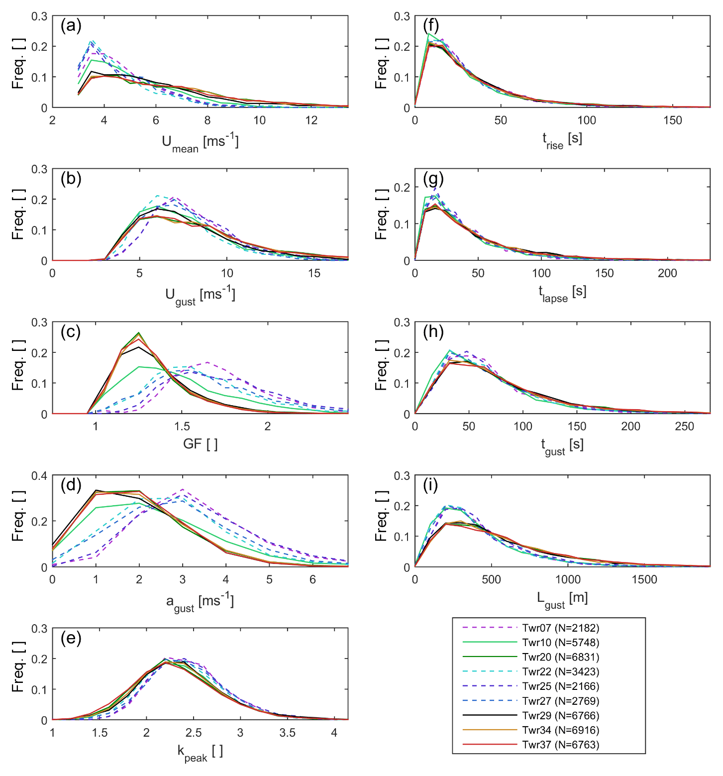
Figure 3 Distributions of gust parameters at each of the nine towers (using data collected at 60 m a.g.l.) for 10 min periods with U_mean>3 m s⁻¹. Valley towers are shown with dashed lines and ridge towers with solid lines. The frames show the (a) 10 min mean wind speed (U_mean), (b) gust magnitude (U_gust), (c) gust factor (GF), (d) gust amplitude (a_gust), (e) peak factor (k_peak), (f) rise time (t_rise), (g) lapse time (t_lapse), (h) gust duration (t_gust), and (i) gust length scale (L_gust). The legend reports the sample size (N) for 10 min periods used to construct the empirical distributions for each tower. The towers are denoted by the color scheme introduced in Fig. 1.

3.3 Spectra and coherences

Power spectral densities (PSDs) of wind speeds from the sonic anemometers and the ZephIR lidars are calculated using Welch's method (Welch, 1967). For the sonic anemometer data this method is applied to 2 h time series of 18 Hz longitudinal wind speed measurements that meet the gust criteria and (separately) those that do not. Spectra are plotted in nondimensionalized form wherein the power at each frequency is multiplied by the frequency and divided by the variance computed from the 18 Hz time series, and the frequency is multiplied by a measurement height (z) of 60 m and the mean wind speed during that 2 h period. Mean PSDs computed for sonic anemometers deployed on all ridge and valley towers are presented for data conditionally sampled by atmospheric stability, turbulence intensity, and wind direction.

Spatial relationships of longitudinal wind speeds from the sonic anemometers (and ZephIR lidars) are characterized in the frequency domain using coherence functions, C_xy, given by the cross-spectral properties:

$$\begin{array}{}\text{(14)}& C_{xy}\left(f\right)={\displaystyle \frac{\left|P_{xy}\left(f\right)\right|}{\sqrt{P_{xx}\left(f\right)P_{yy}\left(f\right)}}},\end{array}$$

where f is frequency, P_xy(f) is the cross-spectral density of x and y, and P_xx and P_yy are the auto spectral densities of x and y, respectively (Bendat and Piersol, 2011). The normalization means that if two time series are perfectly correlated at a given frequency, C_xy(f)=1. Wind speed coherence functions are often characterized using a single-parameter exponential decay function, C_fit,xy (Solari, 1987):

$$\begin{array}{}\text{(15)}& C_{\text{fit},xy}\left(f\right)=\exp \left(-C{\displaystyle \frac{f\cdot d}{U_{\text{mean}}}}\right),\end{array}$$

where C is the decay coefficient and d is the distance between sensors. A nondimensional reduced frequency $\left(\frac{f\cdot d}{U_{\text{mean}}}\right)$ is used herein to facilitate comparison of the coherence functions between sonic anemometers deployed on different towers and with previous research (Solari, 1987; Mehrens et al., 2016). Empirical estimates of a coherence function are influenced (and their accuracy limited) by the number of sub-series used in the cross-spectral density calculation. Hence estimates of C_xy(f) do not decay to zero but to a coherence floor (Mann, 1994). This upward bias of the coherence estimate is the result of the imaginary contribution to the numerator in Eq. (14), which will tend toward zero as the data length increases. This bias can be excluded from the coherence estimate by including only the real part of P_xy(f) in the estimation (Eliassen and Obhrai, 2016). This estimator is also called the co-coherence (CC_xy). Equation (16) is used to estimate coherence functions in the current study.

$$\begin{array}{}\text{(16)}& C_{xy}\left(f\right)\approx {\text{CC}}_{xy}\left(f\right)={\displaystyle \frac{\text{Real}\left(P_{xy}\left(f\right)\right)}{P_{xx}\left(f\right)P_{yy}\left(f\right)}}\end{array}$$

Thus, herein, C values are determined by least-squares fitting of Eq. (15) to the coherence function values, as approximated by the co-coherence. Previous research has indicated large C values are most frequently observed in unstable conditions and that coherence decays quickly with reduced frequency (Kristensen and Jensen, 1979). For 10 min mean wind speeds over water an average value of C=4.3 has been proposed for horizontal separations of <5 km (Vigueras-Rodríguez et al., 2012), and the correlation between two measured time series displaced horizontally asymptotes to a constant value (i.e., the coherence floor) at a normalized frequency ≈ 0.36 (Mehrens et al., 2016). Due to the relatively low sampling rate of the ZephIR lidars (∼ 17 s), coherences of horizontal wind speeds from the ZephIR lidars are calculated over a 72 h period with a fast Fourier transform (FFT) window length of 256 (2⁸), while the coherence functions calculated from the sonic anemometer observations are based on 2 h periods of 18 Hz longitudinal wind speed data, transformed into the frequency domain using an FFT window length of 16 384 (2¹⁴).

Characterization of the height at which the surface characteristics cease to dominate scales of flow in the atmosphere has applications to microscale model verification and validation and is accomplished herein through investigation of the height dependence of the spectral peak associated with the diurnal timescale (f=1 day⁻¹) (Larsén et al., 2018). The magnitude of the diurnal peak, S_p, is calculated as a function of height from the PSDs of wind speeds from all 10 ZephIR lidar measurement heights and sonic anemometer data from the three tallest towers (20, 25, and 29) as follows (Larsén et al., 2018).

1. Calculate the PSD using Welch's method and the longest complete data period.

2. Perform log-smoothing (35 points per decade) of these PSDs by piecewise cubic interpolation.

3. Fit a linear function to each PSD (log S(f) vs. log(f)) to the data in the range $\mathrm{3}\times {\mathrm{10}}^{-\mathrm{6}}<f<\mathrm{2}\times {\mathrm{10}}^{-\mathrm{5}}$ Hz, excluding the value at F_d (frequency = 1 day⁻¹).

4. Calculate three parameters:

   • S_reg (F_d), the value of the linear fit at the daily peak frequency, F_d;

   • (F_d), the value of the PSD at F_d;

   • S_p, the height of the daily peak above the linear background (S(F_d)−S_reg(F_d)).

The reverse height is the height of the minimum value of S_p from each independent measurement and, as described above, is interpreted as the height at which surface-driven processes no longer dominate flow variability.

4 Results

4.1 Wind gust properties and parameter distributions

Mean sustained (10 min) wind speeds (U_mean) are higher at ridge towers than at towers in the valley. The median values are 5.70 and 4.26 m s⁻¹, respectively (Fig. 3a). Tower 10 is an exception to this general pattern because although it is located on the northeast ridge it is sheltered by an area of higher elevation to the north (Fig. 1) and thus experiences flow conditions that are, overall, more like the valley towers. Although the full sample of U_mean values at all towers is best fit by a Weibull distribution (Fig. 2, as at flat sites and offshore; Morgan et al., 2011; Pryor et al., 2004), when a threshold of 3 m s⁻¹ is applied, the resulting samples of U_mean values are lognormally distributed at all towers (Table 2).

In accordance with a priori expectations, gust amplitudes ($a_{\text{gust}}=U_{\text{gust}}-U_{\text{mean}}$) are higher in the valley than along the ridges (Fig. 3d) while U_gust (the maximum 3 s moving average in a 10 min period) exhibits similar values at ridge and valley towers (7.36 and 7.57 m s⁻¹, respectively), with valley towers showing a more peaked distribution and ridge towers exhibiting a longer tail (Fig. 3b). The total sample of U_gust estimates is best represented by either a Weibull distribution, as commonly used in wind turbine modeling (Cheng and Bierbooms, 2001), or a gamma distribution, which has been used in previous work to describe gusts below a canopy (Shaw et al., 1979) (Table 2). Consistent with measurements from moderately complex terrain (Hu et al., 2018), when U_gust is conditionally sampled for U_mean>3 m s⁻¹, it is best fit by a lognormal distribution. Extreme values of U_gust (i.e., 99th percentile (p₉₉), which ranges from 13.2 to 17.1 m s⁻¹ across the towers) are most accurately predicted by the gamma distribution. Parametric estimates of p₉₉ are conservative when derived from the lognormal fit, but are biased low from both gamma and Weibull distribution fits to data from sonic anemometers deployed at or close to 60 m a.g.l. on all towers (Fig. 4a). Consistent with measurements from moderately complex terrain (Hu et al., 2018), a_gust values (i.e., the deviation of the maximum 3 s moving average from the 10 min mean) are best described by a Weibull distribution (Table 2), but 99th percentile values of a_gust (5 to 7.8 m s⁻¹) estimated from the Weibull parametric fit are also nonconservative. While all other distribution types tend to overpredict the 99th percentile gust amplitude value (Fig. 4b), the gamma distribution appears to generate the most representative (but conservative) estimates. Thus, if the upper percentiles of wind gust intensity are of particular interest (e.g., in engineering for wind loading) it may be preferable to use a lognormal distribution to represent U_gust and a gamma distribution for gust amplitude ($a_{\text{gust}}=U_{\text{gust}}-U_{\text{mean}}$).

Although gust magnitude and amplitude are useful for determining the loading force exerted by wind gusts, GFs (i.e., the ratio of the 3–5 s gust magnitude to the sustained wind speed) are frequently used in the meteorological community as a nondimensional intensity index (Krayer and Marshall, 1992) and are sometimes used for assessment of wind hazards (Deaves, 1993). GFs are generally higher in the valley than on the ridge (median GF at valley towers is 27 % higher than those from the ridge towers; Fig. 3c), consistent with the lower U_mean in the valley. GF samples from the 60 m measurement level are best described by the log-logistic distribution (as at a site in moderate terrain complexity; Hu et al., 2018) or lognormal distributions (as in a sample of sites distributed across the eastern United States; Pryor et al., 2014; Table 2).

Table 2 Best-fit distribution types for each gust property (in each 10 min period when U_mean>3 m s⁻¹) for a measurement height of 60 m a.g.l. at each tower. Also shown are results from moderately complex terrain (Hu et al., 2018). The distribution types are referred to as 1–4, where 1 is Weibull, 2 is log-logistic, 3 is lognormal, and 4 is gamma. Distribution types shown in parentheses represent an equivalently good fit (i.e., those with negative log likelihood of less than 0.1 % lower than the best-fit distribution).

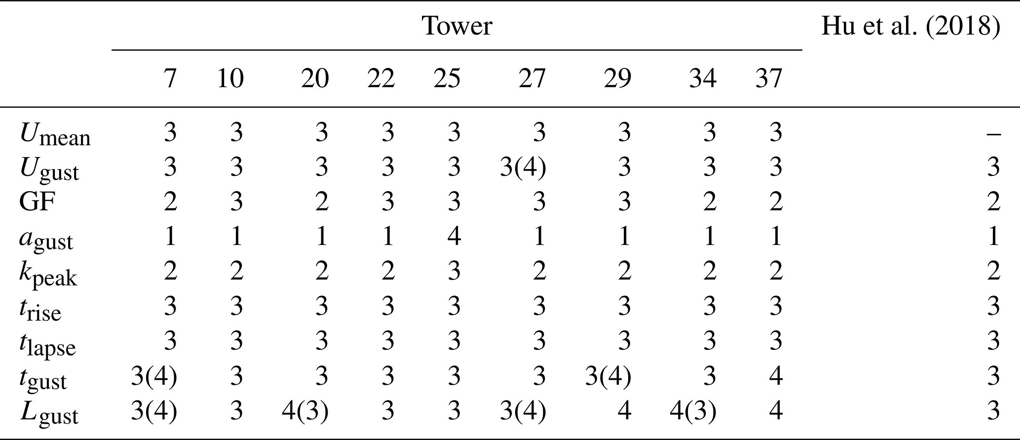
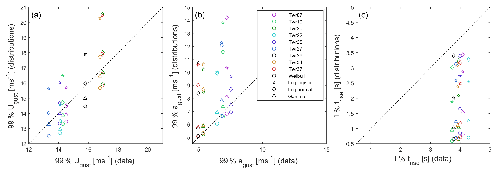
Figure 4 (a) The 99th percentile wind gust magnitude (U_gust), (b) 99th percentile amplitude (a_gust), and (c) first percentile rise time (t_rise) as derived directly from the observations at 60 m a.g.l. and estimated from the parametric distributional fits (shown by the different symbols). The towers are denoted by the color scheme introduced in Fig. 1. The dashed line indicates 1:1 correspondence.

Gust rise time values are similar at ridge and valley towers, median (t_rise) = 24.3 and 23.0 s, respectively (Fig. 3e) and greatly exceed the minimum 3 s averaging window used in the gust timescale calculations performed herein and the 3–5 s averaging period employed by the World Meteorological Organization and National Weather Service. Again, consistent with previous research, t_rise is best fit by a lognormal distribution (Table 2) (Hu et al., 2018). Short gust rise times are of particular interest in the wind energy industry since gusts may ramp up faster than turbine pitch control systems, which may take several seconds to respond, and can mitigate the induced loads (Burton et al., 2011; Kanev and van Engelen, 2010). The first percentile rise times are uniformly near 4 s. This is because the definition used herein sets t≥3 s for the observational estimates, although the distributional fits permit t<3 s (Fig. 4c). The rise time is most accurately estimated using a lognormal distribution fit to the complete sample (Fig. 3f–g), and all distribution types produce conservative predictions of the first percentile (i.e., overestimate the rapidity of the rise; Fig. 4c). Gust lapse times tend to be longer than rise times (by 30 % to 40 %; Fig. 3f) and also conform to a lognormal distribution, consistent with Hu et al. (2018, their Table 2). The asymmetry in the temporal evolution of wind gusts implied by these rise and lapse times indicates that the Ricker wavelet (Mexican-hat) form often assumed in the wind energy industry is not realized (Hu et al., 2018), which has relevance to power control from wind turbines under high wind gust magnitudes (Gottschall and Peinke, 2007). Gust length scales tend to be higher for the ridge towers (with modal values of 200 m (which is similar to the height of the ridges above in the intervening valley) and values of up to 1200–1400 m; Fig. 3g) than in data from the valley towers and to conform to lognormal or gamma distributions with only a small difference in goodness of fit (NLL) between these two distribution types (Table 2).

The results from analyses of data collected in the complex terrain of Perdigão are thus internally consistent across towers in terms of the distributional form that best describes the gust samples and are also generally consistent with analyses of sonic anemometer data at 65 m a.g.l. collected in moderate-complexity terrain (Hu et al., 2018). To the extent distribution types are uniform across the site, and consistent with previous work (as they are for U_gust, a_gust k_peak, t_rise, t_lapse, and t_gust), it is reasonable to conclude that the best-fit distributions identified herein are effective for describing wind gusts in complex and moderately complex terrain. As noted above, these best-fit distributions can be nonconservative when estimating values in the distribution tail, as is the case with U_gust and the Weibull distribution.

Joint distributions of U_gust at different heights on the same meteorological mast (upper-left off-diagonal panels with green boxes in Fig. 5; see other joint distributions of other parameters in the Supplement) indicate large ratios of major to minor axes and thus a strong association of gust magnitude across heights of 10–100 m a.g.l. The aspect ratio (ratio of major to minor axis) of the joint probabilities of U_gust at different heights also exhibits a clear influence from vegetation at the lowest measurement height. For example, in joint distributions of U_gust on Tower 29 the aspect ratio declines from 3.08 (between measurements at 20 and 10 m a.g.l.) to 1.99 (between 100 and 10 m a.g.l.), but above 10 m a.g.l. ranges from 9.66 (between 30 and 20 m a.g.l.) to 3.79 (between 100 and 20 m a.g.l).

Joint distributions of gust length scale at different heights (L_gust, bottom-right off-diagonal panels in Fig. 5) conversely indicate very low ratios of axes length and hence weaker coherence. Joint probabilities of wind gust magnitude (U_gust) and length scale (L_gust) at the same height (i.e., the diagonal in Fig. 5) indicate moderate aspect ratios (1.6 to 1.8) and thus coherence (consistent with previous research; Doran and Powell, 1982), but there is little systematic variation with height. Thus, while gust length scales do not exhibit similarity across heights, there is strong vertical coherence in the magnitude of wind gusts across the layer from 20 to 100 m a.g.l.

Joint distributions of gust magnitudes (U_gust) at 60 m a.g.l. at Towers 20, 22, 34, and 37 (Fig. S1 in the Supplement) indicate very high aspect ratios for values from the three towers (20, 34, and 37) on the southwest ridge (7.6–9.9) but considerably lower values with data from Tower 20 (within the valley, of approx. 3). This again reemphasizes that although the occurrence of individual wind gusts at towers along the ridge is not simultaneous (see conditional probabilities discussed below), the probability distributions of their magnitudes are similar. Conversely, consistent with results shown in Fig. 5, joint distributions of gust length scales and timescales across all towers indicate lower consistency and in some cases near independence (as manifest in small aspect ratios of ∼ 1.07–1.55) (Figs. S2 and S3). A further uniform feature of the joint probability plots is that they exhibit evidence of closer correspondence in peak factor values than GFs both between towers and between heights on a single tower. As shown in Figs. S4 and S5, aspect ratios for peak factor at 60 m a.g.l. between the ridge-top towers vary between 2.8 and 3.6, while those for GFs are 1.8 to 2.1.

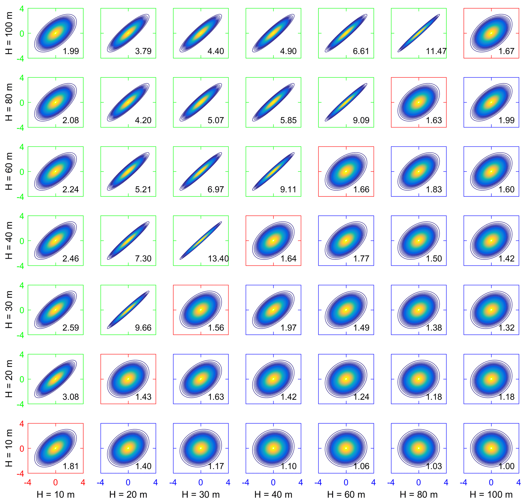
Figure 5 Joint distributions of U_gust and L_gust at different heights (H) from Tower 29. Upper-left off-diagonal panels with green boxes show the joint distributions of U_gust at each pair of heights. Diagonal panels with red boxes show the joint distributions of U_gust and L_gust at the same height. Bottom-right off-diagonal panels with blue boxes show the joint distributions of L_gust at each pair of heights. The number at the bottom-right corner of each panel is the average ratio between the major axis and minor axis of ellipses. There are 99 ellipses corresponding to the confidence levels from 1 % (the innermost ellipse with the warmest color) to 99 % (the outermost ellipse with the coldest color).

4.2 Conditional sampling of wind gust properties

Consistent with previous research, the probability of a wind gust varies systematically with dynamic stability and is higher under near-neutral and unstable conditions (Hart and Forbes, 1999), although gust probability at the valley towers is most similar to the ridge towers during times of very high (>0.25) and very low (<0.1) turbulence intensity (TI) (Fig. 6, column 3). Large values of U_gust tend to occur during stable and near-neutral conditions, especially at the ridge-top towers (Fig. 6, column 1) (stable conditions are also found to be associated with higher U_mean). Consistent with previous research, GFs exhibit only a weak dependence on prevailing stability (Agustsson and Olafsson, 2004), but both GFs and gust length scales scale with TI (Ashcroft, 1994; Greenway, 1979; Hu et al., 2018). Gust length scales are largest under the most unstable conditions, particularly at the ridge towers (Fig. 6), while gust amplitude shows large inter-tower variability, particularly during very stable conditions potentially reflecting the role of orographic wave breaking in inducing high-magnitude gusts (Durran, 1990; Hertenstein and Kuettner, 2005). This is consistent with the finding that U_gust at the ridge towers decreases with increasing TI (from 15 m s⁻¹ at low TI to 10 m s⁻¹ at TI > 0.3) since low TI is likely to occur under stable stratification when orographic forcing of standing waves is most likely to occur. Gust probability also shows a consistent dependence on wind direction and is highest for valley towers during perpendicular flow (Fig. 6, column 2), while under flow parallel to the ridges the empirical distributions of wind gust magnitudes, amplitudes, and GFs are rather similar for valley and ridge towers. This indicates that terrain-induced heterogeneity in wind gust parameters is associated with perpendicular flow and that higher spatial resolution may be required to characterize wind gusts at sites with a high frequency of cross-ridge flow.

Figure 6 Median gust parameters during gusty conditions (U_mean>3 m s⁻¹, a_gust>4 m s⁻¹) at 60 m a.g.l. from ridge (solid red) and valley (dashed black) towers. The data sampled are conditionally sampled by stability classes based on Monin–Obukhov length (column 1), wind direction (column 2), and turbulence intensity (column 3) as measured at Tower 29 (60 m a.g.l.). Vertical whiskers at each data point denote the range of median parameter values for all towers in each class. N values in the second row of x axis labels are the number of 10 min periods in each sample. One gust parameter is shown per row: (a) probability of a gust (i.e., percentage of 10 min periods that meet the gust criteria), (b) gust magnitude (U_gust), (c) gust amplitude (a_gust), (d) gust factor GF, and (e) gust length scale (L_gust).

In Fig. 7, data are conditionally sampled to select only periods when wind gusts occurred (i.e., U_mean>3 m s⁻¹ and gust amplitude > 4 m s⁻¹) and median gust length scale, timescale, and magnitude all increase with height at both ridge and valley towers (Fig. 7). Median gust duration also at the ridge towers increases modestly with height from 58 s at 30 m to 72 s at 100 m a.g.l. This equates to an increase of 14 s over a 70 m height interval (i.e., 0.2 m s⁻¹), which is approximately two-thirds of the value (0.35 m s⁻¹) found for flat terrain (Román, 2017). The increase in gust duration with height is 0.20 s m⁻¹ (Fig. 7e). Median GF and gust amplitudes decrease modestly with height. The median GF decreases from 1.55 at 30 m to 1.5 at 100 m. The change of GF with height is thus smaller than over a flat, homogeneous grassland where GF decreased by 0.2 over a 90 m layer (Suomi et al., 2015; Shu et al., 2016). In contrast to the data from the other meteorological masts, gust amplitudes from Tower 25 tend to increase with height consistent with its location in the lee of a ridge, which causes a pronounced reduction in U_mean but has a lesser impact on U_gust. Turbulence intensities decrease with height and, at the ridge-top towers, reach their minimum value by 80 m a.g.l., indicating that the influence of the ground on this parameter (as well as U_mean, U_gust, and GF) is substantially decreased at elevations more than 80 m above the ridge tops.

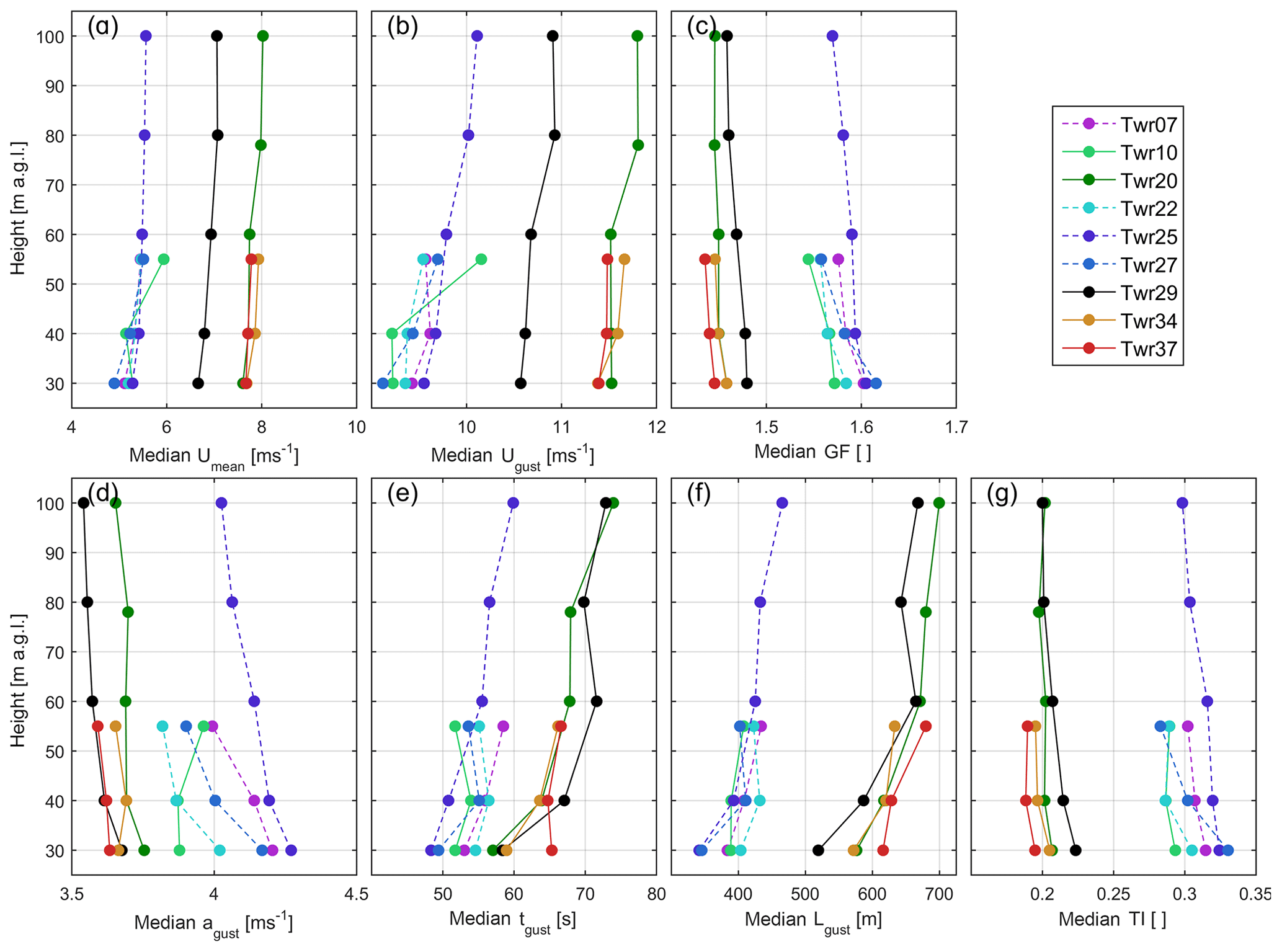
Figure 7 Median values of the gust parameters, by height, at each of the nine towers for 10 min periods that meet the gust criteria: U_mean>3 m s⁻¹ and a_gust>4 m s⁻¹. (a) The 10 min mean wind speed (U_mean), (b) 3 s maximum wind speed (U_gust), (c) gust amplitude (a_gust), (d) gust factor (GF), (e) gust duration (t_gust), (f) gust length scale (L_gust), and (g) turbulence intensity (TI).

Although the ZephIR lidar measurements are disjunct (at approx. 2 s) for each height and are subject to volumetric averaging (over the volume of the annulus swept out by the lidar beam, in a cone 30^∘ from vertical), the probability distribution of U_gust at 100 m a.g.l. derived from measurements with the ZephIR lidar (z423) located close to Tower 25 exhibits accordance with that derived from the sonic anemometer deployed on this tower (Fig. 8a). The U_gust distribution for 100 m a.g.l. from ZephIR z447 (which is 74 m lower and west of the SW ridge) indicates a much higher frequency of U_gust<3 m s⁻¹ than at any of the 100 m towers or ZephIR z423 (Fig. 8a), partly due to sheltering by the SW ridge under northeasterly flow. Vertical profiles of wind gust magnitudes and mean wind speeds follow a power-law form under some circumstances (Brook and Spillane, 1970; Stull, 2012). Median GFs (GF = U_gust∕U_mean) from both the ZephIR lidars and sonic anemometers on the towers also conform to a power law with height (z), although the power-law coefficients and quality of the fit vary among sampling locations and instruments (Fig. 8c). As shown in Fig. 8b, the GF profiles are more linear below the elevation of the ridge tops and data from the ZephIR lidars indicate a higher power-law coefficient consistent with suppression of gust maxima from increased volumetric averaging with height (Suomi et al., 2017). The power-law coefficients for the GF dependence on height are approximately −0.04 to −0.05 in data from the sonic anemometers deployed on the ridge-top towers but are double that for the tower in the valley (25) and are −0.13 and −0.17 in data from the ZephIR lidars (Fig. 8c). For comparison, data from flat surfaces indicate lower GF values and smaller power-law coefficients derived from GF profiles (−0.034 to −0.051, with larger-magnitude values under more stable conditions) (Suomi et al., 2015) than those observed in the current study (Fig. 8c).

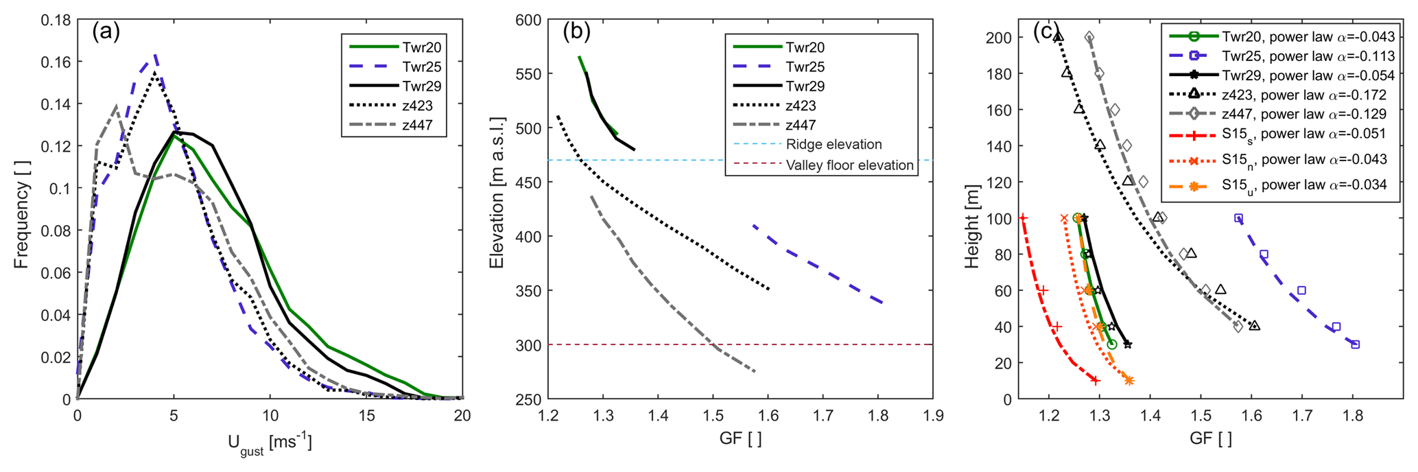
Figure 8 (a) Probability distributions of gust magnitude (U_gust) at 100 m a.g.l. as derived from sonic anemometers deployed on the three 100 m towers and from the ZephIR lidars. (b) Median GF versus height above sea level (a.s.l.) for all 10 min periods with U_mean>3 m s⁻¹ from sonic anemometers and ZephIR lidars. The ridge and valley floor elevations above sea level are shown by the horizontal dashed lines. (c) Power-law fits to median GF as functions of height above ground level for 10 min periods with U_mean>3 m s⁻¹. Also shown are results from measurements over flat terrain (Suomi et al., 2015), under stable (S15_s), near-neutral (S15_n), and unstable (S15_u) conditions.

Gust peak factor (k_peak) derived from sonic anemometer measurements at 60 m a.g.l. greatly exceed 1.7 (Woetmann Nielsen and Petersen, 2001) and results from the empirical expression in Eq. (9) (Wieringa, 1973). Increasing the pre-factor in Eq. (3) from 1 to 2.4 (shown as Wieringa^∗ in Fig. 9) leads to a more conservative approximation, which exceeds 90 % of observed k_peak values for a given sustained wind speed, but the ratio of the 3 s gust amplitude to the standard deviation of the longitudinal wind speed is substantially enhanced in complex terrain and is not well described by either approximation.

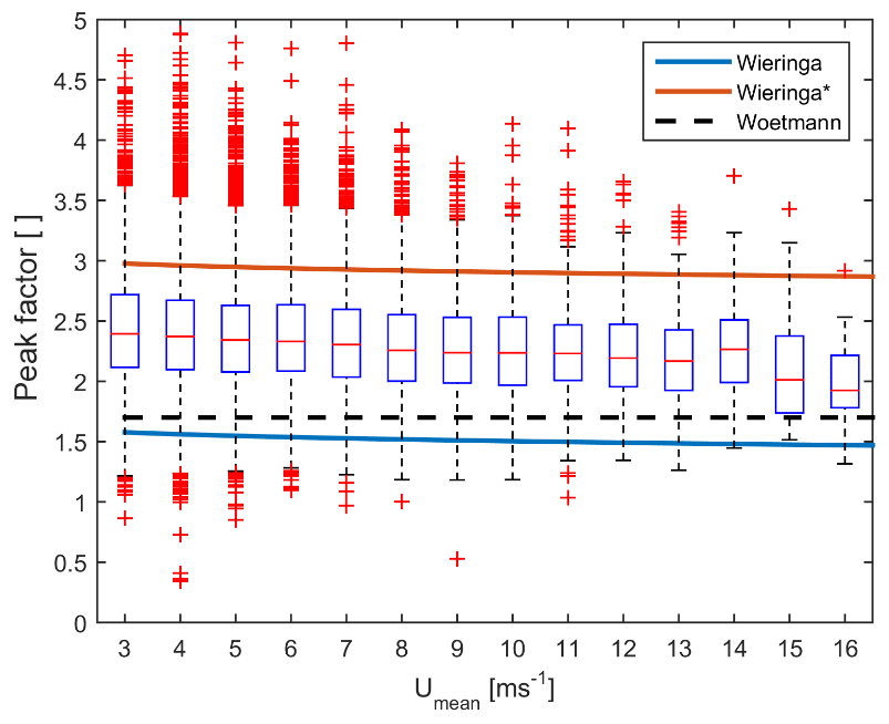
Figure 9 Box plot of gust peak factor (k_peak) estimates at 60 m a.g.l. from all nine towers as a function of U_mean. Also shown are estimates from Eq. (3) (Wieringa, 1973), a revised empirical function in which the leading term in Eq. (3) is increased from 1.0 to 2.4 (Wieringa^∗) and a constant value of 1.7 (Woetmann Nielsen and Petersen, 2001).

4.3 Spatial co-occurrence of wind gusts

The mean marginal gust probability (the average of unconditional gust probability at all sensors) at 60 m a.g.l. across all nine towers is 2.7 % (range of 1.8 % to 5.1 %, Fig. 10a). Thus, on average in any 10 min period at any tower there is a 2.7 % chance that U_mean>3 m s⁻¹ and a_gust>4 m s⁻¹. The mean wind gust co-occurrence probability at 60 m between towers has a mean value of 0.27, indicating that if a wind gust is detected at one given tower in a 10 min period there is a 27 % chance that there will be a gust detected at another given tower in the same 10 min period. When adjacent 10 min periods are included the mean co-occurrence across towers rises to 0.42 (Fig. 10a). The asymmetry in the conditional probabilities shown in Fig. 10 reflects the fact that marginal probability of gusts varies across the study area. For example, the relatively low co-occurrence probabilities seen in Fig. 10c, near the upper-left corner of the panel, indicate that, at Tower 29, given the occurrence of a gust at 20 m, there is a ∼ 30 % chance of observing a gust at 60 m in the same 10 min period (compared to a 2 % marginal gust probability at 80 m). This is distinct from the probability of observing a gust at 20 m given a gust at 80 m (70 %), shown in the lower-right corner of the same panel. The towers are separated by distances of 221 to 1666 m (mean separation of 912 m); thus, although the length scale analysis shown in Fig. 3i indicates that individual wind gusts may not have a sufficient spatial scale to “engulf” two towers, the flow in which these features are embedded is likely to spawn multiple of these coherent transient features across the site. Towers 10 and 20 have the largest overall conditional probability of gust co-occurrence with all other towers (Fig. 10a) in part due to their high marginal wind gust probabilities (4.3 % and 5.1 %, respectively). Conversely, wind gusts at Towers 34 and 37 are not strongly associated with gusts at other towers, especially those located within the valley (Fig. 10a). Towers 20, 34, and 37 are all on the southwest ridge, and their heterogeneity in marginal (1.8 % to 5.1 %) and conditional probabilities (10 % to 40 %) of wind gust occurrence indicate significant spatial variability in flow conditions and the presence of these intermittent coherent structures along the ridge. Indeed the mean gust co-occurrence among these three southwest ridge towers is lower than the site-wide mean. These wind gust co-occurrence probabilities are thus greatly distorted by terrain–flow interactions and are substantially smaller than those reported for flat terrain (of up to 90 % for locations separated by 200 m; Branlard, 2009).

At Towers 25 and 29 (two 100 m towers representing valley and ridge conditions, respectively), the mean intra-tower gust co-occurrence probabilities (computed across heights on the same tower) are 60 % and 55 %, respectively. It is noteworthy that the two ridge-top towers have higher gust probabilities (both conditional and marginal) at their lowest measurement heights, 10 and 20 m, and these probabilities decrease strongly with height (Fig. 10c). Conversely, marginal wind gust probabilities are highest at 80 and 100 m in data from Tower 25 (in the valley) and there is some evidence of a decoupling of data from this tower between heights above and below 80 m as manifested in high joint probabilities of gusts in data from 80 and 100 m and among sonic anemometers at 30, 40, and 60 m a.g.l., but low conditional probabilities between data collected at 80 m and, for example, 40 m.

Figure 10 Co-occurrence of wind gusts in individual 10 min periods among sonic anemometers deployed on different towers (a) or at different heights on the same meteorological mast (b–c). The colors in each of the four panels indicate probability (in 10 probability classes) of a wind gust at anemometer 2 (on the vertical axis) during any 10 min period that also has a gust at anemometer 1 (on the horizontal axis). The marginal probability of a wind gust is also shown along the y axis. (a) Co-occurrence probabilities for gusts at 60 m a.g.l. across all nine towers. Towers are sorted by their distance from Tower 29; colored dots in each square show the probability of co-occurrence when the time window is extended to 30 min. Also shown is the co-occurrence of wind gusts at different heights on (b) Tower 25 and (c) Tower 29.

4.4 Spectra and coherences

Normalized power spectra of longitudinal wind speeds from the sonic anemometers during gust periods differ in three primary ways from the mean spectra derived as the composite of all 2 h non-gust periods. Firstly, during gusty periods the spectral peak is shifted to the left (to lower normalized frequencies), secondly, the spectral peak is more distinct, and lastly, the spectra exhibit lower variance at higher frequencies (normalized frequency > 1) (Fig. 11). This is consistent with the lower-frequency effects (such as terrain forcing and mountain waves) that are associated with gust production being more pronounced during these gusty periods. The relative magnitude of spectral peak at normalized frequencies of 0.07 to 0.17 is greater during gusty periods in data from the valley towers than the ridge towers (Fig. 11a) and is in the same frequency range (i.e., period ≈ 120 s) as in less complex terrain (Hu et al., 2018). At the three tall towers, the proportion of wind speed variance associated with normalized frequencies > 1 decreases monotonically with height, while the share of variance expressed at low frequency increases (Fig. 11b–d) (Kaimal and Finnigan, 1994). Composite spectra during stable and unstable conditions (Fig. 11e) indicate that during stable conditions, the variance at both ridge and valley towers is shifted toward lower normalized frequencies in contrast to previous research in rolling terrain that indicated a shift of variance towards higher normalized frequency during stable conditions (Panofsky et al., 1982). Composite spectra conditionally sampled by wind direction indicate that when the flow is parallel to the ridges (within ± 15^∘ of NW or SE), consistent with results shown in Fig. 6, the power spectra of longitudinal winds from the ridge and valley towers are very similar (Fig. 11f), while during periods of perpendicular flow the variance at the valley towers is shifted to higher normalized frequencies (consistent with the energy cascade induced by topographic forcing and previous work at lower measurement heights (1.6 m) downstream of a smaller obstruction (11.6 m); Panofsky et al., 1982).

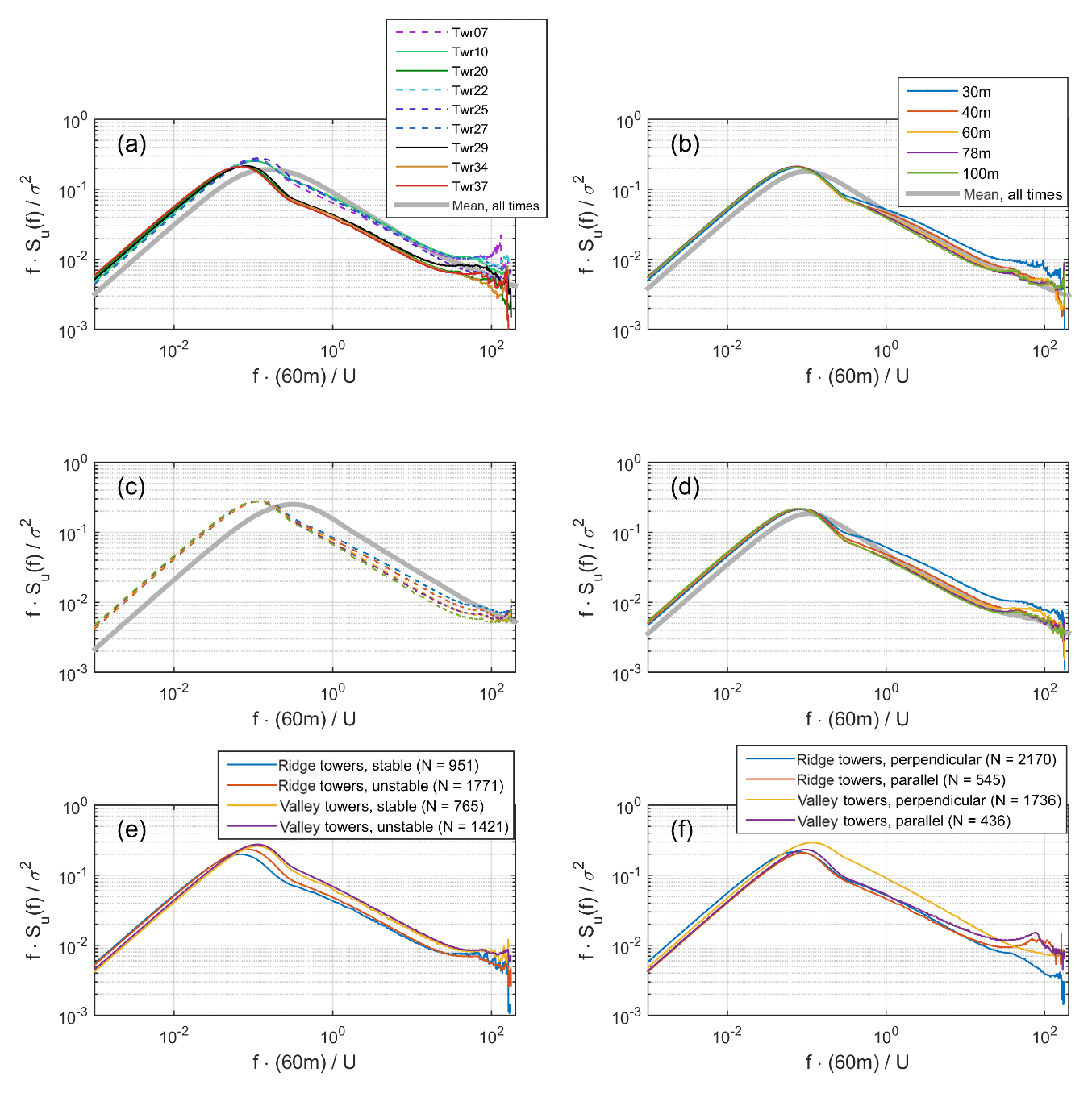
Figure 11 Power spectra of wind speeds during gusty conditions (U_mean>3 m s⁻¹ and a_gust>4 m s⁻¹). (a) Spectra of wind speeds at 60 m a.g.l. on the nine towers. Panels (b–d) show the normalized composite spectra from (b) Tower 20, (c) Tower 25, and (d) Tower 29 from multiple heights. Panels (a–d) also show the mean normalized spectra for all measurement periods (including non-gust periods). (e) Mean normalized spectra at ridge and valley towers, conditionally sampled by stability class, stable (including very stable) and unstable (including very unstable) conditions, and (f) mean normalized spectra at ridge and valley towers, conditionally sampled by wind direction: parallel (±15^∘ of NW or SE) and perpendicular (±15^∘ of NE or SW) to the ridges.

Power spectra of horizontal wind speed computed for all 10 ZephIR lidar measurement heights and from sonic anemometers deployed on the 100 m meteorological masts indicate relatively wide variability in the magnitude of the diurnal peak, S_p, from 0.6×10⁴ to 2.6×10⁵ m² s⁻¹ due to variations in surface forcing across the site and instrumentation differences. Preliminary estimates for the reverse height (i.e., the height of minimum variance at a frequency equal to 1 day⁻¹) derived from the ZephIR lidars (z423 in the central valley and z447 that was deployed outside the ridge–valley system) are approximately 180 m a.g.l. (Fig. 12), which is higher than reported for coastal sites (approx. 120 m a.g.l.; Larsén et al., 2018). Reverse height estimates from sonic anemometers on the ridges (Towers 20 and 29) and ZephIR lidar z423 are approximately 40–80 m above the ridge top (Fig. 12).

Figure 12 (a) Power spectra of horizontal wind speeds at 10 heights from ZephIR lidar z447 and linear fits defining the trend in each near the frequency of 1 day⁻¹. (b) Vertical profiles of the magnitude of the diurnal peak in wind speed variance S_p, from each ZephIR lidar and the sonic anemometers deployed on each 100 m tower. Measurement heights are shown by their elevation above sea level. The towers and lidars are denoted by the color scheme introduced in Fig. 1. Ridge and valley floor elevations are also shown.

Coherence functions of longitudinal wind speed from horizontally separated sonic anemometer pairs do not conform to an exponential form and instead exhibit a marked concave-down section at reduced frequencies below 0.7 (Fig. 13a). Nevertheless, functional values are substantially higher for ridge towers (excluding 10) than for valley towers, indicating greater coherence across the top of the valley than within the valley. Fitted C values (from Eq. 15) range from 1.5 at some ridge-top towers up to 9.7 at Tower 27 (one of the most sheltered towers). These C values, computed for horizontal separation, are toward the low end of C values reported in previous research that indicate C estimates between 5 and 15 and that for sensor separation distance-to-height ratios >2 (which is the case for inter-tower coherences in the current study), the mean decay rate was greater than 19 (Solari, 1987; Larsén et al., 2016). It is possible that the discrepancy in C values with previous research is due to poor fit to an exponential form in coherence functions (Fig. 13a), although it may also reflect faster decoupling of flow regimes in complex terrain. Intra-tower coherences derived using data from different heights relative to data from 60 m a.g.l. are well described by Eq. (12). Coherence functions for the 100 m ridge towers (represented by Tower 29; Fig. 13c) have C values between 9.6 and 14.0, which lie in the middle of the range (C=6 to 16.9) observed in previous work for pairs of sensors separated by a vertical distance (Solari, 1987). These values are higher overall than those measured for longitudinal separation, which is consistent with Taylor's hypothesis that turbulent structures evolve slowly, as they are advected by the mean flow (Larsén et al., 2016). Though Tower 25 had among the highest decay rates of coherence with the reference tower, the intra-tower coherences for Tower 25 exhibit C values of 7.6 to 11.8 (Fig. 13b). Consistent with expectations, the sensors closest to 60 m a.g.l. at each tower have the highest coherence with measurements at 60 m a.g.l., while the measurements at the 30 m a.g.l. sensor (the lowest height included in this analysis) have the lowest coherence values (and highest decay rate). The vertical coherence functions from Perdigão towers decay to their minimum value at a reduced frequency of ∼ 0.3, which is similar to the value of 0.36 calculated for wind over water (Mehrens et al., 2016). Coherence functions derived using wind speeds from ZephIR lidar z423 show slightly larger C values that are derived from sonic anemometer data from the nearby Tower 25 and exhibit high C values between measurements at 60 m a.g.l. and those above 100 m a.g.l., indicating a reduction in the degree to which flow at these heights is coupled (Fig. 13d).

Figure 13 Mean coherence in longitudinal wind speeds as measured by sonic anemometers based on 2 h time series. (a) Mean coherences between Tower 29 and each other tower, for a 60 m measurement height, and exponential fits thereto. (b) Coherences between each height and the 60 m reference height at Tower 20. (c) Coherences between each height and the 60 m reference height at Tower 25. (d) Coherence in horizontal wind speed at each height and the 60 m reference height measured by ZephIR lidar z423.

5 Concluding remarks

The experiment conducted at Perdigão provides an unprecedented data set for studying flow characteristics in complex terrain. Herein we focus on wind gust characteristics as described using 6 months of data recorded at 18 Hz from 51 3-D sonic anemometers deployed on nine tall meteorological masts at heights of 10 to 100 m and two vertically pointing Doppler lidars. Consistent with previous research, analyses presented herein illustrate substantial spatial heterogeneity in the magnitude, scale, and occurrence of wind gusts over an area of approximately 3 km by 3 km (Fig. 1) and reemphasize the complex effects of terrain forcing on near-surface flow.

Nine properties of wind gusts (intensity measures of magnitude, amplitude, peak factor, and GF and scale metrics of rise and lapse time, duration, and length scales) exhibit parent probability distributions similar to those derived from measurements in moderately complex terrain (Hu et al., 2018), indicating that these distributional forms may be generalizable. However, the best-fit distributional forms (selected using negative log-likelihood) underestimate the magnitude and amplitude of intense gusts (i.e., the 99th percentile values). Although the wind gust parameters (including probability of gust occurrence) exhibit similar distributional forms across the site, they differ greatly in terms of the shape and scale parameters of the distributions as applied to data from locations in the valley compared to the ridge tops. Joint probability distributions of the gust parameters indicate high aspect ratios for gust intensity (e.g., gust magnitude; U_gust) across different measurement heights and locations. However, low aspect ratios are evident for gust length scale (L_gust) computed from sonic anemometers deployed at two heights on the same meteorological mast and/or deployed on meteorological masts separated by horizontal distances of 200 to 1600 m (Fig. 5).

GFs measured at Perdigão are larger than those measured in less complex terrain (Fig. 8c; Suomi, 2015) but decrease with height (z) at a rate similar to measurements over flat grassland (Fig. 7c; Shu et al., 2016). While the majority of gust parameters exhibit a decreasing rate of change with z as z increases, t_gust and L_gust show a marked increase between 80 and 100 m. This is consistent with the idea that the spatial scale and timescale of gusts may be more affected by the presence of complex terrain than gust intensity (as measured by U_gust, GF, or a_gust) The rate of decrease in t_gust with height is roughly two-thirds that measured in flat terrain (Román, 2017).

Wind speed spectra during gusty periods (when U_mean>3 m s⁻¹ and gust magnitude (U_gust) >4 m s⁻¹) exhibit a shift toward higher variance at lower frequencies and a more pronounced peak near a reduced frequency ($f\cdot z/U$) of 0.1, indicating that, while individual gusts may not be sufficient to affect 10 min spectra, gusty conditions are associated with a significant change in spectra. The amount of variance in wind speeds associated with the diurnal cycle varies depending on measurement system and location within the study site. Nevertheless, there is evidence that the reverse height (where the first-order effects of heat exchange at the land surface are minimized) is ∼ 60 m above the ridges that enclose the valley.

Gust parameters, and their spatial heterogeneity, are found to vary with atmospheric conditions including wind direction, stability, and turbulence intensity. Differences in observed gust parameters between ridge and valley towers are less pronounced when the flow is parallel to the ridge orientation. Unstable and very unstable conditions (as well as high turbulence intensity) are associated with less ridge–valley differentiation in U_gust magnitudes, suggesting that increased vertical mixing leads to decreased orographic sheltering of the valley towers.

Gust co-occurrences and coherence statistics indicate the presence of large-scale gust phenomena that are simultaneously manifested at the ridge towers but not the valley towers. Gust occurrence across the Perdigão site is significantly influenced by the terrain, resulting in a much lower average gust co-occurrence probability (of 27 %) across towers than those observed in flat terrain (Branlard, 2009). The decay of coherence functions for vertical displacements is in the range found in flat terrain (Solari, 1987; Vigueras-Rodríguez et al., 2012). However, coherences for the large horizontal displacements (>700 m) among towers do not fully conform to an exponential fit (as with those presented in Mehrens et al., 2016) and are characterized by smaller decay coefficients than have been found in research conducted in less complex terrain.

There are clear commonalities in gust properties across the site and among estimates derived using data from sonic anemometers and vertically scanning Doppler lidar. Additionally, co-occurrence probabilities of wind gusts across the site illustrate the very high complexity of flow over what is superficially a simple two-dimensional valley enclosed by two parallel ridges (Fig. 1). These results further indicate that terrain features (and the vegetation canopy) may have a more profound impact on the dimensions of wind gusts than their magnitude. The reverse height (approximately 60 m above the ridge tops) is consistent with a decoupling of flow derived from the coherence functions estimated from the vertically scanning Doppler lidars (as indicated by the step change in C values; Fig. 13d). This is similar to the height at which some gust properties exhibit diminishing dependence on local surface characteristics (U_gust, a_gust and TI; Fig. 7b, g, d), supporting the hypothesis that reverse height is linked to the influence of the ground on wind speed fluctuations on the timescale of gusts. Gust length scales on the ridge tops are frequently similar to the height of the ridge above the intervening valley (which is approx. 175 m deep), and the modal gust length scale measured in the valley is 200 m.

Data collected during the Perdigão experiment and analyses presented herein provide a foundation for improved wind gust characterization in complex terrain. These data also provide an unprecedented opportunity for detailed validation and verification of numerical wind flow models (Butler et al., 2015; Suomi and Vihma, 2018).