Constructing a data-driven receptor model for organic and inorganic aerosol – a synthesis analysis of eight mass spectrometric data sets from a boreal forest site

The interactions between organic and inorganic aerosol chemical components are integral to understanding and modelling climate and health-relevant aerosol physicochemical properties, such as volatility, hygroscopicity, light scattering and toxicity. This study presents a synthesis analysis for eight data sets, of non-refractory aerosol composition, measured at a boreal forest site. The measurements, performed with an aerosol mass spectrometer, cover in total around 9 months over the course of 3 years. In our statistical analysis, we use the complete organic and inorganic unit-resolution mass spectra, as opposed to the more common approach of only including the organic fraction. The analysis is based on iterative, combined use of (1) data reduction, (2) classification and (3) scaling tools, producing a data-driven chemical mass balance type of model capable of describing site-specific aerosol composition. The receptor model we constructed was able to explain 83±8 % of variation in data, which increased to 96±3 % when signals from low signal-to-noise variables were not considered. The resulting interpretation of an extensive set of aerosol mass spectrometric data infers seven distinct aerosol chemical components for a rural boreal forest site: ammonium sulfate (35±7 % of mass), low and semi-volatile oxidised organic aerosols (27±8 % and 12±7 %), biomass burning organic aerosol (11±7 %), a nitrate-containing organic aerosol type (7±2 %), ammonium nitrate (5±2 %), and hydrocarbon-like organic aerosol (3±1 %). Some of the additionally observed, rare outlier aerosol types likely emerge due to surface ionisation effects and likely represent amine compounds from an unknown source and alkaline metals from emissions of a nearby district heating plant. Compared to traditional, ion-balance-based inorganics apportionment schemes for aerosol mass spectrometer data, our statistics-based method provides an improved, more robust approach, yielding readily useful information for the modelling of submicron atmospheric aerosols physical and chemical properties. The results also shed light on the division between organic and inorganic aerosol types and dynamics of salt formation in aerosol. Equally importantly, the combined methodology exemplifies an iterative analysis, using consequent analysis steps by a combination of statistical methods. Such an approach offers new ways to home in on physicochemically sensible solutions with minimal need for a priori information or analyst interference. We therefore suggest that similar statistics-based approaches offer significant potential for un- or semi-supervised machine-learning applications in future analyses of aerosol mass spectrometric data.

1 Introduction

Along with particle size, aerosol chemical composition is fundamental in understanding aerosol physicochemical properties such as hygroscopicity, volatility, optics and toxicity (Bilde et al., 2015; Swietlicki et al., 2008; Zimmermann, 2015). In the past decade aerosol mass spectrometry has provided a way to quantitatively resolve basic chemical composition of aerosol in near real time. This not only enables basic chemical speciation into organic and common inorganic ion species, but also produces a wealth of complex mass spectrometric data. It has since become clear that these data sets, although superficially hard to interpret, are rich in chemical information and their statistical analysis yields considerable new knowledge. However, tapping into this information source requires use of advanced analysis tools and chemometric methods (i.e. “using mathematical and statistical methods to provide maximum chemical information by analysing chemical data”; Kowalski, 1975). Consequently, advanced statistical methods for data reduction have quickly gained traction in aerosol mass spectrometry, and are presently widely used for deconvolution of complex organic mass spectra into their underlying components. Specifically, the positive matrix factorisation algorithm (PMF; Paatero and Tapper, 1994) has achieved a predominant status as the state-of-the-art analysis tool for deconvolving aerosol mass spectrometric data. Factorisation methods such as PMF notably allow for the condensation of information found in high-dimension data matrices into a manageable number of factors, corresponding to aerosol chemical species, sources or processes, for example. Data reduction often additionally allows for improved visualisation, aiding in interpretation of the underlying aerosol chemical phenomena.

In exploratory factor analysis, the principal difficulties often relate to deciding the optimal number of factors, choosing between multiple solutions of mathematically similar quality, and estimating the reliability and uncertainty of the results. Lacking robust but easy-to-use mathematical tools, the selection and interpretation of factorisation solutions remains prone to subjective bias by the analyst. Specifically, while analyst-imposed additional constraints in factorisation may sometimes be required to reduce rotational uncertainty and extract minor factors in data (e.g. Canonaco et al., 2013; Crippa et al., 2014) such procedures are especially prone to analyst-subjective decisions. Evaluation and verification of a factorisation solution thus generally requires meticulous study and understanding of, for example, correlations with auxiliary data, temporal changes and cycles and spectral references. While statistics-driven methods for spectra comparison and classification as of yet remain marginal in aerosol mass spectrometry, they do show promise in their capability to automatically group similar spectra based on their chemically relevant features, producing comparable classifications to those performed manually by expert analysts (Äijälä et al., 2017; Rebotier and Prather, 2007; Freutel et al., 2013).

The overwhelming majority of PMF analyses to date from aerosol mass spectrometer (AMS) have been performed on the organic fraction alone (Zhang et al., 2011). Contrary to popular belief, there exists no tenable reasons to limit chemometric analysis to organic signals, as exemplified by the analyses of Sun et al. (2012) and Hao et al. (2014). Although it requires some additional data preparation and processing, inclusion of inorganics provides additional insight into, for example, salt formation in aerosol. In this work, we apply data reduction and classification methods for analysing organic and inorganic aerosol mass spectral data from several measurement campaigns in the boreal forest. We then derive a comprehensive receptor model resolving the dominant aerosol categories at the site. In addition, by presenting an example of a semi-supervised, statistics-driven analysis of large mass spectral data sets, we hope to pave the way for machine-learning-based data analysis approaches, reducing the need for expert analyst input and subjective judgement at each step.

2 Methods

Our instrumentation, data processing, measurement site and analysis algorithms have been comprehensively described in previous literature, to which we refer in the corresponding sections. Thus, we focus on the new aspects of this work, showing how the individual methods can be connected to form an analysis chain, and to exemplify how chemometric information can be propagated through it. In short, we will first cover the measurement site, SMEAR II (Station for Measuring Ecosystem–Atmosphere Relations) and the sets of data available to us (Sect. 2.1). We then describe our mass spectrometer instrument and preparation of data (Sect. 2.2). In Sect. 2.3, we will briefly go through the various statistical tools and algorithms, covering the basics of data factorisation, classification of spectra using a clustering algorithm and clustering solution evaluation, and detail the pre- and post-weighting involved. Section 2.4 describes typical reference methods for inorganics and nitrate apportionment: an ion balance scheme and a separate parameterisation for estimating organonitrate loading, to provide a comparison for the inorganic speciation from our statistics-based receptor model. Finally, in Sect. 2.5, we present a summarised, step-by-step description of how the methods were combined to produce a receptor model for aerosol composition at the measurement site.

2.1 Measurement site and collection of data

2.1.1 The SMEAR II site

The AMS data of this study were collected at the SMEAR II site in Hyytiälä, southern Finland (61^∘50^′40^′′ N, 24^∘17^′013^′′ E). The site is a well-known and well-equipped atmospheric research station, representing rural, background atmosphere in the boreal forest biome. The site and earlier measurements therein have been extensively described and reported in the literature (e.g. Hari and Kulmala, 2005; Williams et al., 2011; Äijälä et al., 2017).

The environment consists mostly of forests dominated by Scots pine (Pinus Sylvestris) – 90 % of land in the nearest 50 km, and 94 % in the nearest 5 km is forested (Williams et al., 2011).

A large part of the aerosol loading at SMEAR II is attributable to regional biogenic secondary organic aerosol (SOA; Corrigan et al., 2013; Crippa et al., 2014; Allan et al., 2006) and long-range transport from industrial regions in southern Finland, western Russia and central Europe (Kulmala et al., 2000; Patokoski et al., 2015; Niemi et al., 2009; Sogacheva et al., 2005). Regional anthropogenic aerosol sources include the towns Orivesi (pop. 9500; 19 km south) and Tampere (pop. 213 000; 48 km south-west), as well as two sawmills and a pellet factory in the village of Korkeakoski, Juupajoki (7 km east-south-east of the station). The surrounding countryside is sparsely populated (5–10 inhabitants km⁻²), and although emissions from agriculture, traffic, domestic heating, cooking and other combustion sources (saunas, barbecues, agricultural machinery etc.) are limited, they are clearly observable at the station and may increase aerosol loading in often plume-type pollution events. The anthropogenic organic aerosols were further analysed previously (Äijälä et al., 2017).

Table 1 Data sets used in this study and their time frames (dd.mm.yyyy).

Table 2 For months when AMS data were available, percentages indicate the fraction of days with at least one data point.

2.1.2 Data sets

In this study, the aerosol composition was monitored by an AMS between 2008 and 2011, during several short measurement campaigns. Notable larger, intensive campaigns at the time were the EUCAARI project (2008–2009; Kulmala et al., 2009, 2011) and HUMPPA-COPEC (2010; Williams et al., 2011; Corrigan et al., 2013). The sets of data used along with their time frames are shown in Table 1. Data availability by year and month is presented in Table 2.

2.2 Instrumentation, data processing and preparation

2.2.1 The aerosol mass spectrometer (AMS) instrument and basic data processing

The mass spectrometric data for this study were acquired with a Time-of-Flight Aerosol Mass Spectrometer (ToF-AMS), developed by Aerodyne Research Inc. (Billerica, MA, US). AMS instruments in general have been described by Canagaratna et al. (2007), and the compact ToF analyser version (CToF) used in this study by Drewnick et al. (2005). Additional, more specific details related to the specific instrument we used are available in our previous study (Äijälä et al., 2017).

In brief, the AMS instrument sucks sample aerosol from atmospheric pressure to vacuum conditions through an inlet system consisting of a critical orifice and a particle concentrating aerodynamic lens (Liu et al., 2007). The sample aerosol beam is directed at a vaporiser operated at 600 ^∘C, whereby flash vaporisation of non-refractory aerosol components occurs. The resulting vapour is ionised using 70 eV electron impact ionisation – a well-characterised hard ionisation technique, resulting in rather universal and predictable but highly fragmenting ionisation. Finally, the ions are led to an orthogonal extraction reflectron time-of-flight mass analyser, where the ions' mass-to-charge (m∕z) ratios are measured.

The per-amu (atomic mass unit) analyser signal is subsequently quantified based on instrument response calibrations and corrections (among others the correction for relative ionisation efficiency between the species, RIE; Allan et al., 2004; Supplement Sect. S4). Individual, unit-mass-resolution amu signals are then chemically speciated, based on chemical information on fragmentation and air composition (see Allan et al., 2003b, for details). Additional, specific minor modifications to our instrument have been discussed in our previous work (Äijälä et al., 2017).

2.2.2 Data preparation and down-weighting

After basic processing, the data were further prepared, to serve as input for factorisation (described in following Sect. 2.3). The organic and inorganic data and related uncertainties were extracted, and down-weighting of signals performed. The procedure for extraction and preparation of AMS organic signal and related error matrices has been described by Allan et al. (2003b) and Ulbrich et al. (2009).

In short, measurement points or variables with missing data were omitted and error matrices calculated, based on a function accounting for both counting-statistics-induced uncertainty as well as background noise from the detector and electronics. The signals were then down-weighted by multiplying the error-matrix-conveyed uncertainty values for low signal-to-noise ratio (SNR) variables with a scalar: “weak” variables (SNR < 3) were down-weighted by a factor of 2 and “bad” variables (SNR < 1) by 10. The procedure for inorganics (SO₄, NO₃, NH₄, Chl, i.e. sulfates, nitrates, ammonia and chloride species) was similar to that used for the organics (“org”), including for the down-weighting of signals derived from fragmentation calculations. Analogous to the basic procedure of down-weighting “duplicate information” organic signals, e.g. those derived from m∕z 44 Th (mainly ${\mathrm{CO}}_{\mathrm{2}}^{+}$), similarly derived inorganic signal weights were normalised so that their weight of the original plus “duplicate” signals equalled that of the original signal. Finally, the matrices for all the ion species (org, SO₄, NO₃, NH₄, Chl, in nitrate equivalent mass) were combined to form the final input matrices for factorisation, while retaining speciation information in the ion indexing.

2.3 Statistical methods and algorithms

2.3.1 Positive matrix factorisation

For factorisation, we used the PMF model developed by Pentti Paatero and colleagues (Paatero, 1997, 1999; Paatero and Tapper, 1994) and widely used for analysis of AMS data since 2007 (Lanz et al., 2007b; Zhang et al., 2011). In brief, PMF is a statistical model, typically resolving a bilinear linear combination of factor profiles (G) and time series (F) best describing the measured data matrix (X; Eq. 1). The residual matrix E then denotes the portion of data left unexplained by the model (i.e. residual). The PMF model is thus formulated:

$$\begin{array}{}\text{(1)}& {\mathbf{X}}_{\left(t\times v\right)}={\mathbf{G}}_{\left(t\times f\right)}\times {\mathbf{F}}_{\left(f\times v\right)}+{\mathbf{E}}_{\left(t\times v\right)}.\end{array}$$

The brackets indicate matrix dimensions, with v denoting number of variables, t the number of time points and f the number of factors. As shown in Eq. (1), the model can be solved for any f (<v, t), requiring it to be selected by the analyst.

The main features setting PMF apart from other similar factorisation models, and making it particularly suitable for atmospheric aerosol models, are on the one hand the limitation of factor profiles and time series to positive values, hence drastically reducing the amount of rotational ambiguity, and on the other hand the improved error model where the quantity to minimise is the weighted (typically the measurement uncertainty) residual, resulting in higher weight for the variables with better SNR. In PMF, the minimum weighted residual is solved using one of the related algorithms, i.e. PMF2 or Multilinear Engine 2 (ME-2; Paatero, 1999). Of the two algorithms, ME-2 can take in additional equations defined by the user, i.e. constraints the solutions need to adhere to. In this study, when ME-2 constraints were applied to the factor profiles, we set upper and lower bounds for the allowed profile solutions. The bounds were based on variability estimates obtained from earlier analysis, as explained later, in Sect. 2.5. Variability estimate of the final model is available in the Supplement (Fig. S13). For running the PMF and ME-2 algorithms, we used the Igor Pro (Wavemetrics Inc.) based SoFi (v. 4.8) user interface developed by Francesco Canonaco and co-workers at Paul Scherrer Institute (PSI). The interface allows input of the pre-processed data and user-selected parameters, and calls on the solver algorithms (PMF2 or ME-2, depending on assignment) to return a solution to be displayed and analysed in SoFi (Canonaco et al., 2013).

When PMF is used as a standalone method for source attribution, the selection of solution needs to be carefully validated. Sensitivities towards a different number of factors, rotations and initialisation seeds are meticulously analysed, and correlations with auxiliary data are computed. A case is then made for why the selection is the best possible. Contrarily, in our analysis approach, we do not claim to arrive at optimum solutions for individual PMF–ME-2 runs. Instead, we rely on a multitude of data de-convolution runs to uncover the main structures in the ensemble of all data sets, and use statistical classification methods to evaluate the general outlook and commonalities between PMF–ME-2 factors at each analysis phase. As discussed in Sect. 2.5, this trade-off instead enables us to concentrate on best modelling the entirety of all data sets.

2.3.2 Relaxed chemical mass balance model

To harmonise the description of aerosol components, we constructed a constrained receptor model, where all the profile components were constrained. For this purpose we applied a ME-2-based chemical mass balance (CMB) type of model. CMB models are typically used as receptor models for cases where source profiles are known, and only the mass loading information needs resolving (Friedlander, 1973; Gordon, 1988; Hopke, 1991, 2016; Miller et al., 1972). In such mass-conservation-based models, the observed loadings are modelled as a sum of multiple individual sources. Although CMB is often presented mathematically as the sum of loadings (Supplement; Sect. S1, Eq. S1), it can also be thought of as a special case of the bi-linear model described in Eq. (1). Only now the profile matrix (F) is assumed fixed, simplifying the problem to resolving the loading matrix (G) which minimises the residual (E). CMB can be run using the SoFi interface, using the same ME-2 solver as for PMF and ME-2 applications (Canonaco et al., 2013).

In this work, we use a relaxed CMB-like bilinear model (henceforth abbreviated as r-CMB), where all the source profiles are constrained but allowed to vary within narrow limits (derived from variability estimates; see Sect. 2.5; Supplement Fig. S13). In strict technical terms this approach could be labelled “an extremely constrained ME-2 model”, but we choose to use the term “relaxed CMB” to differentiate between the typical use of ME-2 or constraining only part of the profiles, which allows the model considerably more freedom. We regard our use of the model as much closer to the idea of constraining all profiles than (semi-)exploratory factorisation typical for ME-2. The naming also serves to better highlight the conceptual differences between models in the different analysis phases.

Generally, the biggest problems of the CMB models relate to the selection of source profiles, typically from spectral libraries, and handling of their uncertainty. In our use, the anchor spectra as well as the limits for their allowed variabilities are experimentally derived from data, alleviating some of these typical concerns.

2.3.3 k-means clustering

For spectra classification, we selected the k-means algorithm, specifically because in our previous tests it was successful in classifying similar spectral data. The earlier tests additionally yielded useful information on the selection of the dissimilarity metric, as well as algorithm initialisation types and data weighting (Äijälä et al., 2017). The k-means algorithm (e.g. Ball and Hall, 1965; MacQueen, 1967; Steinhaus, 1956; Jain, 2010) is a rather simple, iterative algorithm that partitions a group of objects to a predesignated number of groups or “clusters” based on their relative distances (i.e. dissimilarities). For each iteration, the algorithm assigns all objects to their closest centroids, which are then re-calculated from the mean variable values of the objects in the updated cluster. The aim is to minimise the within-cluster sum of distance (variance) (J) between the objects' (C_n) locations (x_i) and the cluster centroid μ_n they are assigned to (Eq. 2):

$$\begin{array}{}\text{(2)}& J\left(C_n\right)=\sum _{x\in C_n}{∥x_i-{\mathit{\mu }}_n∥}^{\mathrm{2}}.\end{array}$$

The k-means algorithm iteratively converges on (any) minimum of total J (C) obtained by summing over all objects C_n. To increase chances of finding a global minimum, repetitions using different initialisations are used. Specifically, we used the improved stepwise initialisation “kmeans$++$” (Arthur and Vassilvitskii, 2007; available in MATLAB v. 2017a for example, Math Works Inc., Natick, MA, USA).

2.3.4 Spectral similarity and mass scaling

Based on our earlier metric comparison (Äijälä et al., 2017), we used (Pearson) correlation as a metric for spectral dissimilarity (or “distance”, d; Fortier and Solomon, 1966; Mcquitty, 1966):

$$\begin{array}{}\text{(3)}& d\left(\mathit{u},\mathit{v}\right)=\mathrm{1}-{\displaystyle \frac{{\sum }_{i=\mathrm{1}}^n\left({\mathit{u}}_i-\stackrel{\mathrm{‾}}{u}\right)\left({\mathit{v}}_i-\stackrel{\mathrm{‾}}{v}\right)}{\sqrt{{\left({\sum }_{i=\mathrm{1}}^n\left({\mathit{u}}_i-\stackrel{\mathrm{‾}}{u}\right)\right)}^{\mathrm{2}}}\sqrt{{\left({\sum }_{i=\mathrm{1}}^n\left({\mathit{v}}_i-\stackrel{\mathrm{‾}}{v}\right)\right)}^{\mathrm{2}}}}},\end{array}$$

where u and v are the spectra in vector form, with m∕z variables as vector components, and $\stackrel{\mathrm{‾}}{u}$ and $\stackrel{\mathrm{‾}}{v}$ are the arithmetic mean values of u and v.

In clustering mass spectra, data weighting is often applied. Based on previous tests (Äijälä et al., 2017), we applied mass scaling of variables, advocated by Stein and Scott and others (Stein and Scott, 1994; Kim et al., 2012; Horai et al., 2010), giving additional emphasis to higher mass signals. This common practice is based on the idea that higher mass fragment ions are more indicative of their parent ions, and thus the original characteristic composition, while smaller fragments can be produced from a wider variety of molecular fragmentation events. In mass scaling the weighted variables ($\widehat{x}$) are calculated by multiplying the original variables (x) by mass-to-charge-specific weights (w), as presented in Eq. (4).

$$\begin{array}{}\text{(4)}& {\widehat{x}}_{m/z}=x_{m/z}\times w_{m/z};w_{m/z}={\left(m/z\right)}^{s_{\mathrm{m}}},\end{array}$$

where the scaling factor s_m was optimised for each classification separately (Supplement; Sect. S2).

2.3.5 Silhouette metric and post-weighting

The optimisation of mass scaling was based on the silhouette metric (later also abbreviated as “silh”; Rousseeuw, 1987), ranging between −1 to 1 and providing a straightforward, quantitative way to evaluate performance of the classification algorithm. The object-specific silhouette value s_i, defined as

$$\begin{array}{}\text{(5)}& s_i=\left\{\begin{array}{ll}\mathrm{1}-{\displaystyle \frac{a_i}{b_i}};& \mathrm{for}{a}_i<b_i\\ \mathrm{0};& \mathrm{for}{a}_i=b_i\\ {\displaystyle \frac{b\left(i\right)}{a\left(i\right)}}-\mathrm{1};& \mathrm{for}{a}_i>b_i\end{array}\right.,\end{array}$$

where a_i corresponds to the mean distance to other objects in the same cluster, and b_i similarly to the mean distance to objects in the nearest neighbouring cluster. A silhouette value close to unity indicates the object is well clustered, while a value close to zero indicates the classification is uncertain, and the point is likely situated in-between two possible centroids. A negative cluster value is indicatory of possible misclassification. Silhouette values can be calculated for any single cluster as the arithmetic mean of the cluster members' silhouettes, or similarly as a mean over all objects, to evaluate the quality of the clustering solution as a whole.

In order to mitigate the k-means algorithm's known sensitivity to outliers, and to improve handling of between-cluster samples, we applied a simple post-processing to all cluster centroids and variability calculations: the centroid spectra and variabilities were calculated as weighted averages ($\widehat{\mathit{\mu }}$), and weighted standard deviations (${\widehat{\mathit{\sigma }}}^{\mathrm{2}}$; Eq. 6) respectively, instead of the normal unweighted values (similar to Äijälä et al., 2017). As weights, we used the object specific silhouette values s_i>0 (Eq. 5):

$$\begin{array}{ll}{\displaystyle }& {\displaystyle }\widehat{\mathit{\mu }}={\displaystyle \frac{{\sum }_{i=\mathrm{1}}^N{s}_i{v}_i}{\sum _{i=\mathrm{1}}^N{s}_i}};{\widehat{\mathit{\sigma }}}^{\mathrm{2}}={\displaystyle \frac{{\sum }_{i=\mathrm{1}}^{N}s{\left(v-\mathit{\mu }\right)}^{\mathrm{2}}}{\sum _{i=\mathrm{1}}^N{s}_i}};\\ \text{(6)}& {\displaystyle }& {\displaystyle }{s}_i=max(s_i,\mathrm{0}),\end{array}$$

where v_i are the cluster member objects (spectra) This procedure down-weights likely misclassified objects (silhouette <0) to zero, and penalises the more uncertain or questionable assignations (low silhouette) compared to the decidedly well-clustered objects (silhouette close to unity). Singleton clusters were omitted from this calculation, and their variability was thus left undefined.

2.4 Standard approximations for aerosol inorganic speciation and organonitrate

2.4.1 Ion balance model for inorganics

Aerosol inorganic chemical speciation is better understood than the organic speciation, due to much lower diversity of the chemical compounds involved. A variety of aerosol inorganic equilibrium models exist and are typically used as modules in atmospheric meteorological and air quality models. However, performing thermodynamic equilibrium calculations is computationally demanding (e.g. Fountoukis and Nenes, 2007) and requires a good deal of auxiliary data on thermodynamic conditions and chemical activities. Due to the complexity of the models and increased data needs, simpler approximations are often used in connection with AMS inorganic speciation. In the following ion-balance-scheme description, we denote the respective AMS ion species molar concentrations in square brackets (e.g. [${\mathrm{NH}}_{\mathrm{4}}^{+}$], [${\mathrm{NO}}_{\mathrm{3}}^{-}$], [${\mathrm{SO}}_{\mathrm{4}}^{\mathrm{2}-}$]).

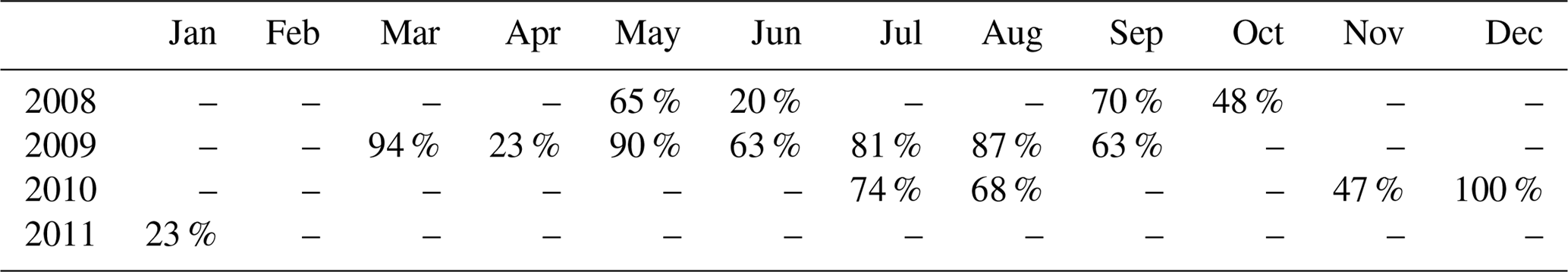
A typical salt formation approximation used for AMS results is the Hong et al. (2017) ion pairing scheme, used in aerosol volatility and light scattering models, for example (Hong et al., 2017; Zieger et al., 2015). The Hong et al. (2017) scheme is based on similar approximation of Gysel et al. (2007), which in turn is a simplification of the more extensive model by Reilly and Wood (1969). We modified the Hong et al. (2017) scheme to additionally allow organonitrate (orgNO₃) and speciate any leftover [${\mathrm{NH}}_{\mathrm{4}}^{+}$] as its own class (“excess ${\mathrm{NH}}_{\mathrm{4}}^{+}$”). The full scheme is available in the Supplement (Sect. S3), and a schematic description is presented in Fig. 1.

Briefly, in the scheme we apply, ${\mathrm{NH}}_{\mathrm{4}}^{+}$ is first combined with ${\mathrm{SO}}_{\mathrm{4}}^{\mathrm{2}-}$ to form ammonium bisulfate and/or ammonium sulfate depending on the relative concentrations of [${\mathrm{NH}}_{\mathrm{4}}^{+}$] and [${\mathrm{SO}}_{\mathrm{4}}^{\mathrm{2}-}$]. Any leftover [${\mathrm{NH}}_{\mathrm{4}}^{+}$] then combines with [${\mathrm{NO}}_{\mathrm{3}}^{-}$], until all [${\mathrm{SO}}_{\mathrm{4}}^{\mathrm{2}-}$] and [${\mathrm{NO}}_{\mathrm{3}}^{-}$] is fully consumed in forming (NH₄)₂SO₄ and NH₄NO₃. After this point, any leftover [${\mathrm{NH}}_{\mathrm{4}}^{+}$] is considered “excess” and assigned to a separate class. For comparability with other models, any nitrate not in NH₄NO₃ is labelled organic. Despite the label, we note this class not only encompasses organonitrates, but also any NO⁺ fragment signal from amines and N-containing organics and may even contain influences of other inorganic nitrate species, such as KNO₃, which are not considered separately in this simple model. Finally, since chloride loadings at the measurement site are generally negligible, neutralisation of hydrochloric acid (H₂O : HCl) was not included to keep this scheme rather simple. We note that ion balance schemes depending on relative ion abundances, such as the one described here, can be sensitive to measurement uncertainties (e.g. errors in RIE values) of these ratios. The topic is further discussed in the Supplement (Sect. S4)

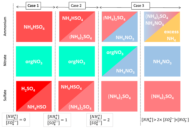
Figure 1 Schematic representation of the inorganic apportionment scheme. The scheme is divided into three cases according to the ratio of [${\mathrm{NH}}_{\mathrm{4}}^{+}$] to [${\mathrm{SO}}_{\mathrm{4}}^{\mathrm{2}-}$]. [${\mathrm{NH}}_{\mathrm{4}}^{+}$] first combines with [SO₄] to form NH₄HSO₄ (Case 1), then further to (NH₄)₂SO₄ (Case 2). In these cases, any nitrate observed is considered organic. In Case 3 leftover [${\mathrm{NH}}_{\mathrm{4}}^{+}$] then associates with [${\mathrm{NO}}_{\mathrm{3}}^{-}$] until all the inorganic anions are neutralised. Any leftover [${\mathrm{NH}}_{\mathrm{4}}^{+}$] is labelled as “excess ${\mathrm{NH}}_{\mathrm{4}}^{+}$”. A full description of the scheme is given in the Supplement (Sect. S3).

2.4.2 Kiendler-Scharr parameterisation for organonitrate

The organic nitrate estimate in the above model is very sensitive to calibration parameters (see Supplement Sect. S4). Therefore, in addition to the ion-balance-based scheme above, we additionally calculated a particulate organonitrate mass estimate (orgNO_3 mass), based on the nitrate fragmentation ratio-based parameterisation of Kiendler-Scharr et al. (2016; Farmer et al., 2010):

$$\begin{array}{ll}{\displaystyle }& {\displaystyle }{{\mathrm{orgNO}}_{\mathrm{3}}}_{\mathrm{mass}}=\\ \text{(7)}& {\displaystyle }& {\displaystyle }{{\mathrm{NO}}_{\mathrm{3}}}_{\mathrm{total}}{\displaystyle \frac{\left(\mathrm{1}+R_{{\mathrm{orgNO}}_{\mathrm{3}}}\right)x\left(R_{\mathrm{measured}}-R_{\mathrm{calib}}\right)}{\left(\mathrm{1}+R_{\mathrm{measured}}\right)x\left(R_{{\mathrm{orgNO}}_{\mathrm{3}}}-R_{\mathrm{calib}}\right)}},\end{array}$$

where R refers to the ratio of nitrate signals at 46 and 30 Th, i.e. R=NO₃ (m∕z 46 Th) : NO₃ (m∕z 30 Th), for organonitrate (“orgNO₃”), NH₄NO₃ calibration (“calib”) and ambient measurement (“measured”), respectively. For the parameterisation, we applied an ion ratio R_calib=0.42, taken as the average of mass-spectrum-based AN calibrations (Supplement Sect. S6). An $R_{{\mathrm{orgNO}}_{\mathrm{3}}}$ value of 0.1 was used, based on the estimate by Kiendler-Scharr and co-workers for their observations on organonitrate spectral properties (Kiendler-Scharr et al., 2016).

2.5 Constructing a data-driven r-CMB receptor model

As stated in the Introduction, one of the aims of our work was to derive a robust, harmonised receptor model for the measurement site via explorative analysis. Considering the large amount of campaigns during different seasons, resulting in changing aerosol source contributions and mass spectral profiles, factorisation needed to be performed on a per-campaign (data set) basis. However, instead of performing traditional PMF complete with correlation analysis, source validation and the various sensitivity analyses separately, which would be an arduous task even for a single measurement set, we used the large amount of data sets to our advantage. Instead of optimising individual factorisations, we constructed an r-CMB model applicable to all data sets. A similar task of constructing a semi-exploratory synthesis aerosol model, albeit one applying a different methodology, was undertaken and reported by Sofowote et al. (2015).

Figure 2 A flowchart illustrating the analysis using combined methodology. After initial data collection and preparation, statistical analysis is performed in three phases (P-I to P-III). Each phase limits the freedom given to factorisation from completely free (PMF) to nearly fully constrained (r-CMB). Finally, we evaluate and interpret the r-CMB model from an aerosol chemical perspective.

To derive the anchors and constraints for a synthesis r-CMB model, we analysed the data in three phases (P-I to P-III; Fig. 2), each consisting of factorisation, classification and silhouette-based post-weighting of anchor spectra and their allowed variabilities. The allowed variabilities were constrained by setting upper and lower bounds (the estimated variability ranges from the previous phase) for factor profiles. In Phases I and II, a fixed number of 10 factors were resolved. This amount of factors was semi-arbitrarily chosen, and in our case likely to be somewhat above the optimal amount for most data sets, leading to over-resolved factor solutions. However, unlike in traditional PMF analysis, we can use additional statistical diagnostics and post-processing options available to deal with potential fallout of unrealistic factor splitting (i.e. classification for identifying outliers and post-processing down-weighting or nullifying their influence). Sensitivity to initialisation seed was examined by performing all runs using 10 initialisation seeds, and generally selecting the solution with lowest normalised residual. In rare cases of a physically unrealistic solutions such as the one with the lowest residual (e.g. only NH₄ species in a factor), a higher residual solution was chosen instead. We conclude the solutions were generally insensitive to seed selection, especially for the factors with non-negligible mass contribution.

2.5.1 Phase I: anthropogenic aerosols

In phase I (P-I), we performed unconstrained factorisation for all the eight data sets. With 10 factors this resulted in a total of 80 factors of mass spectra. We then determined the dominant spectra classes using k-means clustering. To that purpose, we applied optimised mass scaling for improved data structure, and used silhouette diagnostics to evaluate the optimal number of clusters. We identified the known, common anthropogenic aerosol classes from the silhouette-weighted cluster centroids. This is also an approach advocated by Crippa et al. (2014) in their similar work on a synthesis analysis of several data sets.

For a cluster centroid to qualify as an anchor for further phases of our analysis, we applied the following two criteria: (1) the spectra forming the cluster were present in multiple (≥3) data sets, and (2) the spectra were interpretable chemically and had adequate support from previous studies in the form of literature and/or calibrations. We note that defining what constitutes ”interpretable” or “adequate support” is inevitably an analyst (subjective) decision, so we endeavour to make our reasoning transparent in the respective discussion sections. Adhering to criterion (1) also means that factors showing up only for one to two campaigns, due to special conditions (emission, meteorology etc.), are omitted from the final r-CMB model. We will briefly cover some of the more interesting “outlier observations” in Sect. 3.4. At the end of phase I, a number of constrained anchor spectra and within-cluster-variabilities were obtained. In this case, these corresponded to four anthropogenic classes, which will be discussed in more detail in the results section.

2.5.2 Phase II: biogenic, secondary organic aerosols

Using the anchors and within-cluster variabilities, we re-ran factorisation as in P-I, except now partly constrained (ME-2; 4 of 10 factors constrained using anchors from P-I). In phase II, we focused on analysing the remaining free factors, likely corresponding to the biogenic and assumedly more variable factors (Canonaco et al., 2015; Crippa et al., 2014). The procedure for classification and the selection criteria for the (assumedly) biogenic SOA in this phase were the same as in phase I.

Due to the data-driven analysis approach, specifically the constrained factors being selected from phase I, we do not expect major changes between phase I and phase II (P-II) results. While arguably the methodology could be further developed to constrain the r-CMB components directly from the phase I result, phase II of our analysis currently serves several purposes: (1) it should narrow down the solution space for improved description of the various SOA types, by constraining the anthropogenic, assumedly primary aerosols. (2) Compared to P-I, the allowed solutions are more similar for all data sets in P-II, which reduces the scatter of the factorisation solutions. This reduces the spectral variability (uncertainty) arising from the analysis process itself, allowing us to iteratively converge on more realistic limit values for the constraints. Ultimately, the limits should reflect the actual, natural chemical variabilities within the aerosol types. (3) Similarity of results between successive, un- or semi-constrained phases allows evaluation of stability, reliability and repeatability of the method, so that it is not e.g. overly sensitive to rotational ambiguity or initialisation parameters of algorithms. This is important since the method described here is new, and its robustness needs to be demonstrated, but less so in potential later use.

2.5.3 Phase III: final, constrained receptor model

In phase III (P-III), we constructed the r-CMB receptor model. In this phase, all the factors were constrained using anchors and variabilities from the previous phase result. The number of components in the final r-CMB model, in our case 7, was equal to the total number of selected aerosol types in phase II. With these model constraints, we performed runs for each of the eight data sets separately. Using the resulting 8×7 factor profiles, we determined the likely range of variability for the aerosol types, and calculated final, silhouette-weighted reference spectra for the components by performing a final round of clustering.

3 Results and discussion

In Sect. 3.1, we briefly describe the results from analysis phases I to III (P-I to P-III; corresponding to Sect. 3.1.1 to 3.1.3) but concentrate more on the receptor model results and their interpretation (Sect. 3.2). Finally we will compare our results with reference methods (Sect. 3.3). Comparison results are available in the literature for organic aerosol components (Sect. 3.3.1), and in Sect. 3.2 we will compare inorganic speciation with the alternative inorganic attribution methods, described in Methods (Sect. 2.4). Finally, we briefly describe some of the outlier observations which contain potentially interesting chemical information (Sect. 3.4).

When interpreting and identifying aerosol components, we evaluate spectral similarity using the same similarity metric (mass scaled correlation) as for the clustering (Eqs. 3 and 4). We thus report mass scaled squared correlation coefficients ($r_{\mathrm{s}}^{\mathrm{2}}$) between reference spectra and our corresponding final spectrum for the class (P-III silhouette-weighted centroids; s_m=1.81). For easier comparability, all ratios and fractions of signals presented in the following sections are similarly calculated from the corresponding final spectra (P-III).

3.1 Receptor model construction steps

3.1.1 Phase I: identification of anthropogenic aerosol components

In phase I, we performed unconstrained PMF runs using 10 factors for all 8 data sets separately. The resulting 80-factor spectra were subsequently clustered. Maximal data structure (silhouette 0.56) was achieved at mass scaling s_m=2.12 for 17 clusters (for details on silhouette analysis, see Supplement, Sect. S2). The eight clusters with largest population for the phase I solution are shown in Fig. 3, and the rest in Sect. 3.4, where outlier observations are further discussed. Generally, the solutions agreed closely on the largest clusters, lending credibility to the robustness of the approach. The solutions differed mainly regarding outlier classification, which is of secondary importance for our r-CMB model, since outliers are discarded from the model.

Figure 3 The eight largest clusters for P-I classification of factorisation results. Cluster centroids (coloured bars) and variabilities (error bars) are silhouette-weighted averages and standard deviations for the cluster members. The main anthropogenic aerosol types were identified as clusters no. 2 (“Ammonium sulfate”, AS), no. 4 (“Hydrocarbon-like organic aerosol”, HOA), no. 5 (“Biomass burning organic aerosol”, BBOA) and no. 8 (“Ammonium nitrate”, AN). Cluster number, silhouette and population (n) are shown in panel titles.

Unsurprisingly, the classification returns two large clusters of organic aerosol resembling the ubiquitous low-volatile oxidised organic aerosols (no. 1; LV-OOA) and semi-volatile oxidised organic aerosol (SV-OOA; e.g. Aiken et al., 2007; Jimenez et al., 2009; Zhang et al., 2011). Comparing to library spectra, the aerosol type dominated by m∕z 44 Th (${\mathrm{CO}}_{\mathrm{2}}^{+}$) (no. 1) best matches with LV-OOA and OOA-I (oxidised organic aerosol, a historical label corresponding to LV-OOA; Aiken et al., 2008; Zhang et al., 2011) spectra from Paris ($r_{\mathrm{s}}^{\mathrm{2}}=\mathrm{0.97}$; Crippa et al., 2013), Zurich (0.96; Lanz et al., 2007a; Crippa et al., 2013) and Borneo rainforest (0.99; Robinson et al., 2011) as well as the average LV-OOA calculated from 15 Northern Hemisphere data sets (0.94; Ng et al., 2010). Cluster no. 3 is characterised by a high m∕z 43 Th signal (C₂H₃O⁺; Aiken et al., 2008) and correlates with SV-OOA and OOA-II (Aiken et al., 2008) spectra from Pasadena (0.74; Hersey et al., 2011), Borneo (0.86; Robinson et al., 2011) and the 15-data-set average (0.76; Ng et al., 2010) as well as the laboratory-generated SOA spectra generated from typical pine forest emitted volatile organic compounds (e.g. α-pinene, 0.81; α-terpinene, 0.83; terpinolene, 0.84; Bahreini et al., 2005). Abiding by the typical naming convention of AMS-derived aerosol types, we label these species LV-OOA (cluster no. 1) and SV-OOA (no. 3).

Figure 4 Final silhouette-weighted reference spectra (coloured bars) and variabilities (error bars) for the r-CMB model components.

The solution also contains a large cluster (no. 2) with spectra dominated by ammonium and sulfate ion species. This is in agreement with ammonium sulfate being a main component of ambient aerosols. Although it also contains trace amounts of other species, we name the (NH₄)₂SO₄-dominated aerosol class (no. 2) ammonium sulfate (AS) for brevity.

The main nitrate-containing spectra are divided into two clusters (no. 6 and no. 8). The divisive feature seems to be the ratio of m∕z 46 to 30 Th signals (i.e. R_measured in Eq. 7), which is much higher in cluster type no. 8 (0.44±0.11) versus for no. 6 (0.08±0.07; P-III; see Supplement Sect. S5 for error estimate). We note once more that these characteristic values for clusters are from the final model (P-III; Fig. 4), as outlined before. Based on the literature we interpret the split to correspond to the division between nitrogen in the form of inorganic (ammonium) nitrate (AN) and organic nitrogen, matching with previous AMS observations (Hao et al., 2014; Farmer et al., 2010; Kiendler-Scharr et al., 2016). The interpretation of cluster no. 8 as AN is additionally corroborated by its similarity to spectra from pure ammonium nitrate calibration for the instrument, available in the Supplement (Sect. S6). On average, the brute-force single-particle (BFSP; Drewnick et al., 2015) AN calibrations performed for the instrument yielded an R_calib (Eq. 7) ratio of 0.49±0.05 (mean ± standard deviation), while an MS mode calibration returned an R_calib of 0.42. Similarly to naming of the AS class, we use labels organic nitrogen (ON; cluster no. 6) and AN (cluster no. 8) for the nitrate-dominated aerosol types. The ON cluster is further discussed in Sect. 3.3.2. The label ON was chosen to differentiate between the (presumably) organic-nitrogen-dominated aerosol class (ON), and the part of NO₃ ion species deemed likely to be organonitrate (orgNO₃).

A fraction of the organic signal observed at m∕z 44 Th for inorganic salt classes (AS and AN) may be explained by an ${\mathrm{CO}}_{\mathrm{2}}^{+}$ artefact induced by thermal decomposition of inorganic salts (Pieber et al., 2016). For ammonium nitrate, the proportion of organic signal at m∕z 44 Th to total nitrate signal is 2.9 % (P-III). Pieber et al. (2016) estimate a contribution of 3.4 %, suggesting most of the organic signal observed in AN may arise from this artefact. This proposition is further discussed in the Supplement (Sect. S6).

Two of the clusters (no. 4 and no. 5) seem related to anthropogenic (primary) organic aerosol types. Cluster no. 4 has a similar spectrum as the hydrocarbon-like-organic aerosol (HOA) spectra from the AMS spectral database (Ulbrich et al., 2009) and closely matches, among others, HOA reported by Zhang et al. (2005) for Pittsburgh ($r_{\mathrm{s}}^{\mathrm{2}}=\mathrm{0.91}$) and the average of 15 de-convolved HOA spectra reported by Ng et al. (2010; $r_{\mathrm{s}}^{\mathrm{2}}=\mathrm{0.89}$). The spectra also exhibits high similarity with traffic emission spectra of diesel bus exhaust (0.86), lubricating oil (0.82) and fuel (0.75), reported by Canagaratna et al. (2004).

Cluster no. 5 features high signals for ions typical of biomass burning organic aerosol (BBOA, e.g. Alfarra et al., 2007) and cooking organic aerosol (COA, e.g. Mohr et al., 2012). The spectra features the marker signals of levoglucosan (Cubison et al., 2011; Schneider et al., 2006) at m∕z 60 (${\mathrm{C}}_{\mathrm{2}}{\mathrm{H}}_{\mathrm{4}}{\mathrm{O}}_{\mathrm{2}}^{+}$) and 73 Th (${\mathrm{C}}_{\mathrm{3}}{\mathrm{H}}_{\mathrm{5}}{\mathrm{O}}_{\mathrm{2}}^{+}$) along with chloride ions (at m∕z 35 and 36 Th) and a high fraction of signal at m∕z 55 Th (C₃H₃O⁺; Mohr et al., 2012), pointing to cooking and/or biomass burning emissions. The highest similarities to library spectra (de-convolved via PMF) are found with COA (Mohr et al., 2012, for Barcelona, $r_{\mathrm{s}}^{\mathrm{2}}=\mathrm{0.70}$; Crippa et al., 2013 for Paris, $r_{\mathrm{s}}^{\mathrm{2}}=\mathrm{0.59}$) and BBOA (e.g. 15-data-set average reported by Ng et al., 2010, $r_{\mathrm{s}}^{\mathrm{2}}=\mathrm{0.51}$) and BBOA de-convolved by Crippa et al. (2013, for Paris, $r_{\mathrm{s}}^{\mathrm{2}}=\mathrm{0.50}$). Similarity to SV-OOA library samples are also moderately high (e.g. Ng et al., 2010, 15-data-set average, $r_{\mathrm{s}}^{\mathrm{2}}=\mathrm{0.59}$).

The differentiation between HOA versus BBOA or COA can often be resolved even from unit resolution spectra, using the f₅₅-to-f₅₇ ratio (Mohr et al., 2012), and the differences in mass spectral fingerprints higher up on the m∕z axis (resolvable using mass scaling; Äijälä et al., 2017). However, the distinction between COA and BBOA aerosol types is much more delicate due to very high unit mass resolution spectral similarity for higher m∕z variables, (e.g. $r_{\mathrm{s}}^{\mathrm{2}}=\mathrm{0.79}$ for COA and BBOA reported by Mohr et al., 2012). The main difference between the COA and BBOA aerosol types is the absolute level signals from levoglocosan fragments, the quantitative interpretation of which is difficult due to (1) levoglucosan production being determined by combustion temperature (Shafizadeh, 1984), (2) levoglucosan originating both from BBOA and COA (Mohr et al., 2012), and (3) levoglucosan sinks being potentially considerable in the atmosphere (Hoffmann et al., 2009), which affects transported aerosol in particular. Due to the remote location of the measurement site and general prevalence of BBOA over COA in urban aerosol loadings (e.g. Daellenbach et al., 2017) we conclude that BBOA is more likely the dominant component for this aerosol type, so we will use the class label “BBOA” for brevity. Due to high spectral similarity, we find it extremely likely that any COA contribution would be apportioned to this class, but without the benefit of high-mass-resolution data, the convolution seems insolvable at this time.

Cluster 7 spectrum offers little in terms of unique spectral features, and it appears as though it could be represented as a combination of the more distinct AS (no. 2), LV-OOA (no. 1) and ON (no. 6) aerosol types. It is unclear whether this class represents an actual aerosol chemical type, or whether it is due to incomplete resolving of the aforementioned species in the PMF model. We note that the organics part of AS, LV-OOA and ON are all highly oxidised, which may imply similar levels of aging and thus similar origins for these species. Organic spectral components are further analysed and discussed in Sect. 3.2.2.

Based on this interpretation and evaluation of criteria outlined in Sect. 2.5, we decided to select the following as the main representative anthropogenic aerosol types: ammonium sulfate (cluster no. 2, n=10, silhouette =0.91) ammonium nitrate (no. 8, n=5, silh = 0.48), hydrocarbon-like organic aerosol (no. 2, n=6, silh = 0.65) and biomass burning organic aerosol (no. 5, n=6, silh = 0.36). The silhouette values can be taken to represent separation distance from neighbouring aerosol types. For comparison, silhouette values for some of the anthropogenic organic aerosol types are available in Äijälä et al. (2017), but to our knowledge no precedent exists for mixed or inorganic aerosols. Generally, the more “unique” the spectra of a group and the higher the within-cluster cohesion, the higher the silhouette.

3.1.2 Phase II: classification of biogenic secondary organic aerosols

In the second phase of our analysis, ME-2 factorisations were run for 10 factors for all the data sets. We constrained 4 out of the 10 factors with the anchors and variabilities for anthropogenic aerosol types, derived from the previous phase (AS, AN, HOA, BBOA). The resulting 80-factor profiles were again extracted and classified. The classification solutions featured generally higher silhouette values than in the first phase, which is at least partly explained by constrained spectra being forced to conform to their set limits. The highest total silhouette (0.66) was obtained for 15 clusters (at s_m=2.41). Again, the inter-solution variability for the solutions inspected was low for the main classes. The phase II solution is available in the Supplement (Fig. S4). Overall, the solution very closely resembles the result from phase I (Fig. 3).

The expected LV-OOA (no. 1; n=14; silh 0.64) and SV-OOA (no. 3; n=9; silh 0.44) aerosol types again rank among the most typical classifications. Their moderate silhouettes reflect higher variability within these classes, corresponding to results from earlier studies (e.g. Canonaco et al., 2015), and/or closer proximity to neighbouring aerosol types, than for the AN, AS or HOA types. The result may suggest seasonal or other data-set-specific variability for SOA, which supports partitioning the data on a per-campaign basis. In accordance with typical AMS organic aerosol classification conventions laid out by Aiken et al. (2008) for example, we opt for two classes of oxidised aerosols. We thus select clusters no. 1 and no. 3 (P-II) to represent LV-OOA and SV-OOA (Aiken et al., 2008; Jimenez et al., 2009) respectively.

For P-III of our analysis, we additionally fix the organic nitrogen class, (ON, P-II cluster no. 8). Irrespective of the exact chemical composition and label of this aerosol component, we assess that there is enough literature support (among others Kiendler-Scharr et al., 2016; Farmer et al., 2010; Drewnick et al., 2015; Murphy et al., 2007; Hao et al., 2014) for inclusion of nitrogen-containing aerosol types other than AN to warrant the inclusion of this class. In any case, the classification of nitrate signal at m∕z 30 Th to a distinct class seems statistically robust, as exhibited by its emergence as a free factor in both P-I and P-II solutions. Due to the importance of nitrogen-containing species in SOA composition and formation (e.g. Kiendler-Scharr et al., 2016; Berkemeier et al., 2016) we find it an important aerosol class to include, examine and further interpret. The mixed cluster no. 7 also emerges for four data sets, but with notably low silhouette (0.18), suggestive of low within-cluster cohesion. As we still lack a distinct chemical interpretation for this class, beyond the hypothesis of incomplete resolution of aged aerosol species in factorisation, we will not include the mixed class (no. 7) in our final receptor model.

3.1.3 Phase III: final r-CMB receptor model

In the final phase (P-III) of constructing our r-CMB receptor model, we used seven factors which were all constrained with the profiles and allowed variabilities from the previous phase (P-II, AS, LV-OOA, SV-OOA, BBOA, ON, HOA, AN). The ME-2 algorithm was tasked with resolving the factors' temporal behaviour.

To derive final characteristic spectra for the model components, as well as to study the variability of spectra in the solutions, we once more applied the same clustering procedure and silhouette analysis as for previous phases. The maximal structure (silh 0.85) was achieved for the seven-cluster solution (s_m=1.81), which was to be expected considering ME-2 was run with seven rather strictly constrained factors in this phase. With silhouette weighting applied, we obtain the final spectra and variabilities (Fig. 4). We note that this final clustering and weighting step mainly serves to provide an estimate of variability within each aerosol type but also yields final spectra to be used as library references for the outcome of this work. Details of the solution of the r-CMB model are discussed in following sections, from the perspective of mass attribution (Sect. 3.2.1) and spectral characteristics (Sect. 3.2.2). Diurnal cycles of the components for the entirety of data are available in the Supplement (Fig. S12). Due to the rural setting of the site and the generally long transport times of aerosol before reaching the site, diurnal cycles for the various aerosol types are not as characteristic as they would be for urban measurements (for example temporal trends of HOA and BBOA). Also due to seasonal differences, the variability between data sets is considerable, resulting in high uncertainty in interpretation. The daily cycles are likely a mixed product of source emissions, boundary layer dynamics and aerosol temperature response. While of interest, disentangling these processes is beyond the topic of this study.

3.2 Overview of r-CMB model results

3.2.1 Mass attribution and “default” AMS chemical speciation for r-CMB components

Tabulation of final explained variations (EVs; Paatero, 2000; Canonaco et al., 2013) for the r-CMB model is shown in Table 3. The seven-component r-CMB model explains 83±8 % of the variation in loadings, when variation from low-SNR variables is included, and 97±3 % when only residuals of variables with SNR >2 are considered. The components with lowest loadings (ON, HOA, AN) explain around 4 % to 5 % of variation, which seems to roughly match the general rule of thumb of PMF–ME-2 being able to extract components of around 5 % of contribution (Ulbrich et al., 2009).

Table 3 Explained variations (EV, in percent) for the r-CMB model.

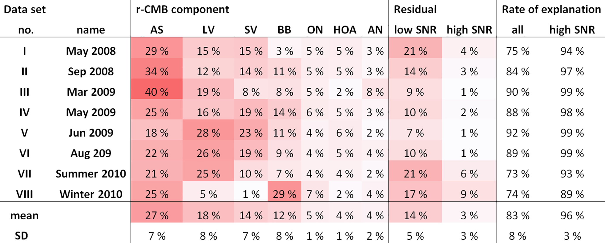
Figure 5 “Default” chemical speciation for r-CMB components: mass loadings (a) and relative contributions (b) of default species in components. Apportionment of default species to r-CMB components by mass (c) and relative contribution (d).

Model results for campaign VIII, especially regarding BBOA, are very different from other data sets, including the other cold season results available in data set III, for example (Fig. S5). Upon closer examination, we attribute the VIII anomaly at least partly to pronounced surface ionisation effects, discussed more in Sect. 3.4. While we consider the r-CMB results for campaign VIII too unreliable for use in models or further studies, we decided not to omit data set VIII, since other AMS data are likely also affected by the same processes, albeit to a lesser degree. The attribution of anomalies to exact processes is very difficult, and surface ionisation effects remain hard to quantify. We hope that reporting our results in full also furthers the discussion of surface ionisation in the AMS, and potentially helps other AMS users observing similar observations.

The composition of our r-CMB components is shown in Fig. 5b, and the same in absolute mass units in panel (a). The opposite visualisation, i.e. attribution of default species into r-CMB components, is similarly given for absolute mass concentration and relative units in Fig. 5c and d. Unlike mass spectral variables and estimated EV, where signals at m∕z are in units “nitrate equivalent mass” (RIE not applied), all mass concentrations reported are corrected for relative ionisation efficiency (see Supplement, Sect. S4).

Generally, the separation between the inorganic r-CMB components (AS, AN) and organics (LV-OOA, SV-OOA, BBOA, HOA) seems clear (Fig. 5). Ammonium nitrate and sulfate components consist primarily of inorganic ion species (81 % to 84 %), while for organic components the inorganic ion species contribution is small (LV-OOA: 8 %, SV-OOA: 8 %, BBOA: 6 %, HOA: 3 %). However, extensive oxidation of organics in aerosol typically results in the formation of organic acids (Yatavelli et al., 2015; Vogel et al., 2013; Duplissy et al., 2011), and we hypothesise that organic salt formation with [${\mathrm{NH}}_{\mathrm{4}}^{+}$] could account for the notable 5 % mass contribution of ammonium to this aerosol type.

Figure 6 Mass attribution in the default AMS speciation scheme (a) and by r-CMB components (b) for all eight data sets combined. Values are (data set length-weighted) averages for all data combined. Absolute mass concentrations are in units (µg m⁻³).

Explanations for the observed mixing of ion species can include (1) mixed emission profiles at sources, variabilities within a source type, as well as collocation of sources; (2) atmospheric processes, such as mass transfer between the species by evaporation, condensation (e.g. Ye et al., 2016) or coagulation; and (3) PMF or r-CMB modelling uncertainties. We will discuss the relative ratios and neutralisation balances of inorganic ion species in Sect. 3.3.2, in relation to inorganic salt formation scheme. The interesting exception to the rather clear-cut ion species separation is the ON component, which contains 40 % of NO₃ species ions, and 41 % of ions defined as organic. The possible interpretations for this distribution are further discussed in Sect. 3.3.2

As for the organics–inorganics division, the two speciations (default vs. r-CMB) give similar results (Fig. 6). For all the data sets combined, the default organic ion species (“org”) explains an average 57 % of total aerosol mass at the site. Similarly, combining the mass of all organic-dominated components (LV-OOA, SV-OOA, BBOA, HOA and ON) results in 60 % mass fraction versus 40 % explained by ammonium nitrate (5 %) and ammonium sulfate (35 %) salts. The per-data-set mass apportionment is presented in the Supplement (Fig. S9).

3.2.2 Spectral characteristics of organic components

As discussed above, despite the mixing observed, the inorganic aerosol classes generally seem separate from organic aerosols. The scaled correlation values between inorganic and organic spectra are extremely low (Supplement Sect. S8, Tables S1 and S2), indicating near-zero similarity and clear-cut separation between the inorganic and organic aerosol types by the clustering algorithm. For inter-correlations between the organics-dominated aerosol classes, the picture is somewhat more complex.

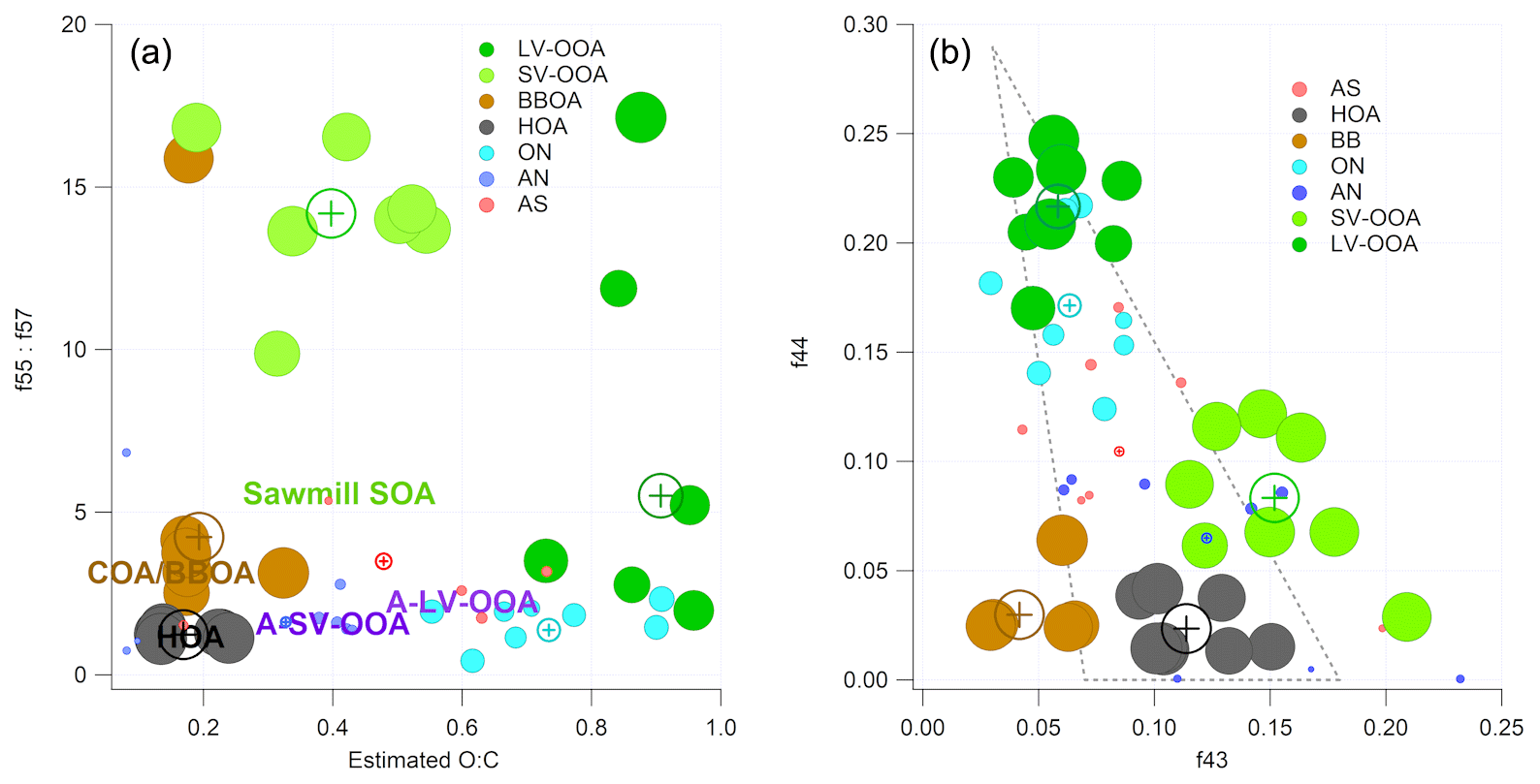
Figure 7 (a) P-III (r-CMB) solution – cluster projections onto a f₅₅∕f₅₇ (Mohr et al., 2012), O : C (estimated, Aiken et al., 2008) plane. Circles correspond to the members of the cluster and the cross markers to cluster centroids. The text markers indicate respective positions of anthropogenic organic aerosol types from Äijälä et al. (2017). Marker size indicates organic mass fraction in spectra. Axes are truncated. (b) P-III solution, projected onto the f₄₄–f₄₃ plane (i.e. the “Sally's triangle” plot; Ng et al., 2011). Circles correspond to objects in clusters and the cross markers to cluster centroids. Marker size indicates organic mass fraction in spectra. A dotted line marks the area where most laboratory data for organic aerosol falls (Ng et al., 2010).

To understand the drivers for the separation of the organic aerosol types, we visualised the phase I (unconstrained PMF) and phase III (r-CMB) classification results with a projection of the clustering solutions onto a plane defined by an axis corresponding to estimated oxidation level and another connected to source type (P-III in Fig. 7; P-I available in the Supplement, Fig. S6). Similar to Äijälä et al. (2017), we describe the oxidation level of the organic fraction of each component using the oxygen-to-carbon ratio (O : C) parameterisation of Aiken et al. (2008), and use the ratio of f₅₇ : f₅₇ to imply source type. The O : C generally separates LV-OOA and SV-OOA species from each other and from the fresher aerosol classes. The f₅₅ : f₅₇ ratio is typically used for differentiation between HOA and COA or BBOA (Mohr et al., 2012) but equally seems to set apart the biogenic SOA types from the anthropogenic aerosols (Äijälä et al., 2017). This is due to the low signal of m∕z  57 Th, a typical anthropogenic spectral marker, originating from ${\mathrm{C}}_{\mathrm{4}}{\mathrm{H}}_{\mathrm{9}}^{+}$ and C₃H₅O⁺ compounds (Mohr et al., 2012; Zhang et al., 2005).

The LV-OOA aerosol type, characterised by the dominant m∕z 44 and 28 Th signals, is usually considered a highly oxidised aerosol type that results from the oxidation of SV-OOA and various fresh emissions (among others Canonaco et al., 2015). The f₅₅ : f₅₇ ratio of LV-OOA is considerably lower than for SV-OOA in both solutions, indicating the inclusion of other sources beyond the f₅₇-poor biogenic SOA contribution. SV-OOA, on the other hand, has the highest f₅₅ : f₅₇ ratio of the classes, hinting at the predominantly biogenic origin of the SV-OOA at the site. The difference is further amplified for phase II and III solutions compared to the unconstrained PMF. We hypothesise that this change can result from improved differentiation between SV-OOA and the BBOA species (in P-II), as these aerosol types may be difficult to separate initially due to similar oxidation level and features of the spectra ($r_{\mathrm{s}}^{\mathrm{2}}=\mathrm{0.34}$; Table S3). The SV-OOA is characterised by the non-oxygen-containing ions at m∕z 29, 43 and 55 Th (Mohr et al., 2009), as well as mass-to-charge m∕z 53 Th signal (${\mathrm{C}}_{\mathrm{4}}{\mathrm{H}}_{\mathrm{5}}^{+}$) typical of boreal forest biogenic backgrounds (e.g. Corrigan et al., 2013). The ${\mathrm{NO}}_{\mathrm{2}}^{+}/{\mathrm{NO}}^{+}$ ratio of 0.10 for nitrate-containing SV-OOA reported by Hao et al. (2014) matches our observations for the nitrates in SV-OOA (${\mathrm{NO}}_{\mathrm{2}}^{+}/{\mathrm{NO}}^{+}$ of 0.11±0.15; Eqs. 7 and S5). This may indicate the presence of organonitrate species in the SV-OOA factor.

We also projected the P-I and P-III solutions to the (f₄₄–f₄₃) plane (P-III in Fig. 7; P-I in the Supplement, Fig. S6), to produce a result comparable to the triangle plot by Ng et al. (2010). The result indicates a clear separation between the low and semi-volatile aerosol types, as well as the primary combustion aerosols (HOA, BBOA), and the spectral shifts from phase 1 “bulk PMF” results to those of the final r-CMB model.

As stated in Sect. 3.1, the spectra of BBOA and HOA aerosol types match the previously published observations. The HOA spectrum is characterised by the ion series C_nH_2n+1 (m∕z 29, 43, 57, 71, 85, 99 Th etc.) and C_nH_2n−1 (m∕z 41, 55, 69, 83, 97 Th etc.) resulting from alkanes and aromatics from traffic emissions (diesel exhaust, lubricating oil; Chirico et al., 2010; Mohr et al., 2009; Canagaratna et al., 2004). The biomass burning organic aerosol levoglucosan marker signals at m∕z 60 (${\mathrm{C}}_{\mathrm{2}}{\mathrm{H}}_{\mathrm{4}}{\mathrm{O}}_{\mathrm{2}}^{+}$) and 73 Th (${\mathrm{C}}_{\mathrm{3}}{\mathrm{H}}_{\mathrm{5}}{\mathrm{O}}_{\mathrm{2}}^{+}$) (Cubison et al., 2011; Schneider et al., 2006; Elsasser et al., 2012) are clearly identifiable in the BBOA spectra (Figs. 3, 4) and set this class apart from HOA and SV-OOA with some similar features. The contribution of often biogenic signals at m∕z 53 Th is also lower for BBOA than for the biogenic, semi-volatile SOA. The pronounced signal from aromatic rings (tropyllium cation ${\mathrm{C}}_{\mathrm{7}}{\mathrm{H}}_{\mathrm{7}}^{+}$) at m∕z 91 Th is a typical result of fragmentation of aromatic hydrocarbon compounds (Lindon et al., 2016). As stated previously, we presume the BBOA class also encompasses any COA contributions, which are likely unresolvable as a separate class due to high spectral similarity (0.79; Sect. 3.1.1).

In terms of spectral characteristics, the organic contributions of AS and AN classes fall somewhere between the distinct organic classes and offer little in terms of significant organic markers. Notably, the organics in the ON class exhibit some of the characteristics of LV-OOA and feature generally high f₄₄. This may indicate a high degree of oxidation of the organics for this aerosol type (Aiken et al., 2008). However, alternative plausible interpretations exist: AMS response from oxidation products of amine compounds and amine-nitrate salts feature similarly high f₄₄ (Murphy et al., 2007) as does a typical amine fragment ion C₂H₆N⁺ (McLafferty and Turecek, 1993). Furthermore, as discussed in Sect. 3.3.2, an equally plausible explanation would be inorganic nitrate salts such as KNO₃ (from biomass burning for example; Li et al., 2003) contributing to this class in the form of the Pieber et al. (2016) thermal decomposition artefact. The contribution of m∕z 55 and 57 Th signals to the ON species are both low and the ratio 1.37 of f₅₅ : f₅₇ is much lower than for the biogenic aerosol species. Without more detailed analysis, and due to the uncertainties surrounding the origins of this aerosol type (Sect. 3.3.2), it is difficult to say with any certainty if this is due to anthropogenic nature of this aerosol, or for example due to fragmentation pattern of characteristic organic compounds in this aerosol type.

3.3 Comparisons with reference methods

3.3.1 Comparison with “traditional” ME-2 analysis for aerosol organic component

In order to evaluate the performance of the source apportionment approach presented in this study for organic aerosol, we compare our results to results only relying on the organic mass spectral fingerprints. Specifically, two data sets covered in this study (data sets II and III; Table 1) were also included in the Crippa et al. (2014) analysis, which allows us to compare factorisation results directly. We chose to compare the Crippa et al. (2014) results to ours from data set II. We note that while there are minor differences in the pre-processing and corrections for data covered in Crippa et al. (2014), the factorisation input is very similar in both cases. The ME-2 model used by Crippa and co-workers included only the organic spectra and apportioned its mass to four factors: LV-OOA, SV-OOA, BBOA and HOA. The latter two components were constrained using a HOA profile from an urban aerosol study in Paris (Crippa et al., 2013) and an average BBOA of those extracted for Mexico City, Mexico, and Houston, USA (Ng et al., 2011). The allowed variability around these anchors for all variables (m∕z) was 5 % (HOA) and 30 % (BBOA).

We compared the solutions for Crippa et al. (2014) factorisation to our r-CMB model solution data set II, both for loadings (Fig. 8) and profiles (Fig. 9). Generally the solutions correlated highly – the loadings (F) and profiles (G) for LV-OOA (F: r²=0.92; G: $r_{\mathrm{s}}^{\mathrm{2}}=\mathrm{0.96}$) and SV-OOA (F: 0.94; G: 0.99) agreed the closest, whilst the HOA also had high similarities (F: 0.85; G: 88). The BBOA factor or component correlated markedly less (F: 0.63; G: 0.42), which we hypothesise to be due to differences in the anchors used, COA likely attributed to this class, high spectral similarity between SV-OOA and BBOA, and the generally low loadings of BBOA observed at SMEAR II.

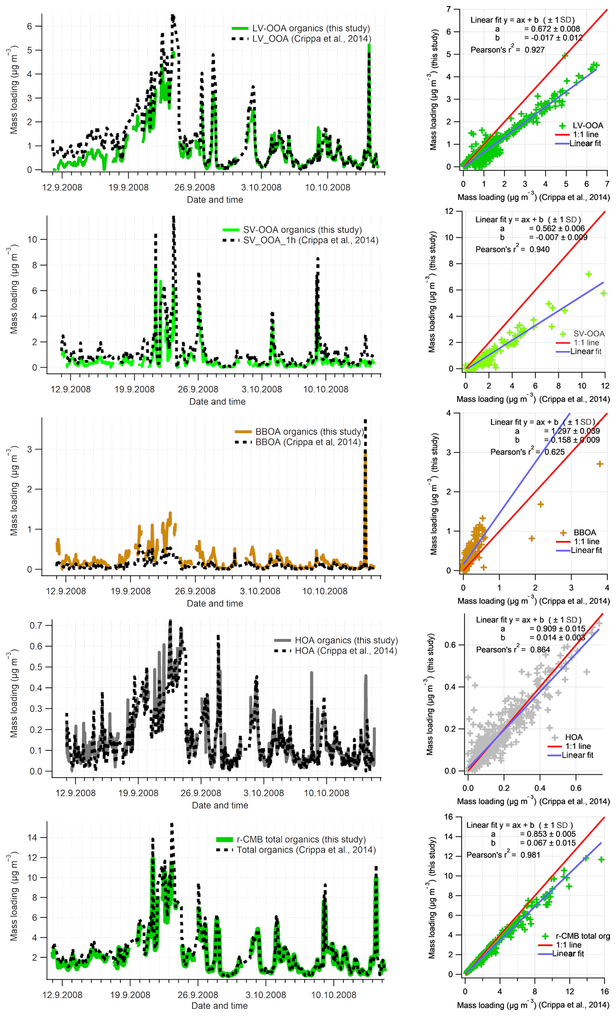
Figure 8 Time series comparison of aerosol organic component with Crippa et al. (2014) for the September 2008 campaign (data set II). For comparability, only the organic part of r-CMB model components are considered. Data from this work have been averaged to 1 h resolution. Organics in other r-CMB components (AS, AN, ON) are taken into account for the total amount but not shown separately. Discrepancy in total organics loading is due to differences in pre-processing values (e.g. ionisation efficiency, collection efficiency).

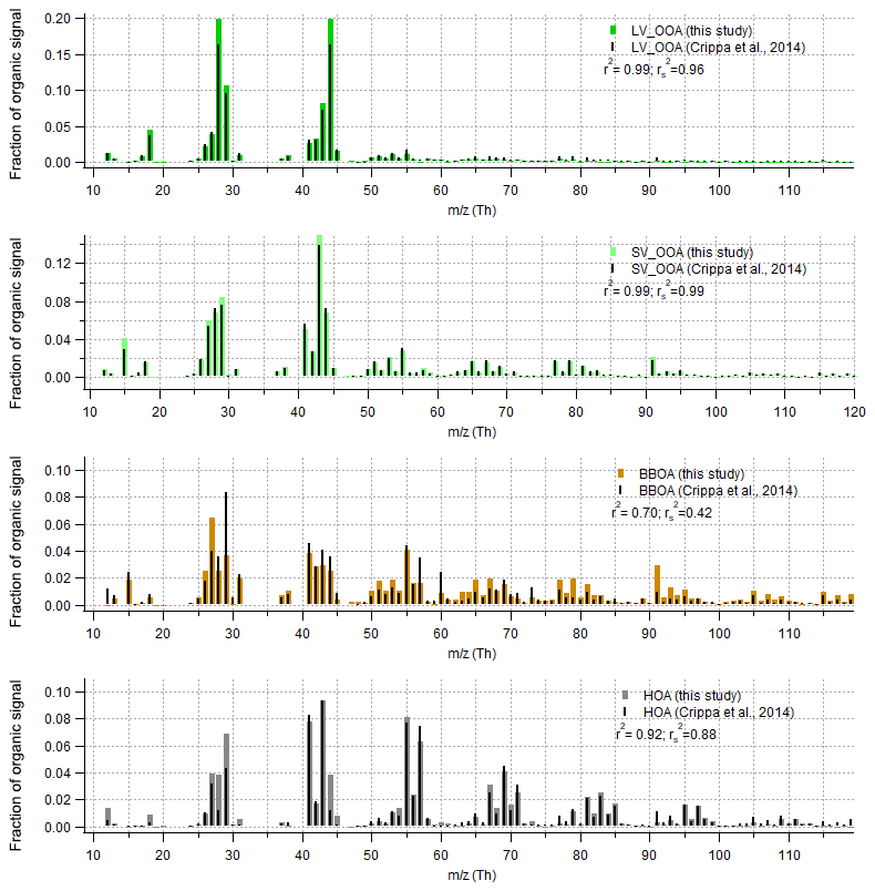
Figure 9 Comparison of organic part of spectra with Crippa et al. (2014) for data set II. The r-CMB model results from this study are shown in colour, and the Crippa et al. (2014) spectra in black. For comparability, the Crippa et al. (2014) spectra were corrected for a difference in fragmentation tables used (included m∕z 28 Th, updated to modern calculation of m∕z 16, 17 and 18 Th organic signals) and total signal subsequently re-normalised to unity. Spectra similarity is evaluated using Pearson's squared correlation coefficients: unscaled (r²) and with mass scaling ($r_{\mathrm{s}}^{\mathrm{2}}$).

The discrepancy in distribution of absolute mass for the LV-OOA and SV-OOA components, indicated by the sub-unity slope, suggests the r-CMB model attributes a part of the organic mass from the SOA factors into BBOA, AS, AN and ON components, while HOA is represented rather identically in both models. A difference in mass distribution between the results is to be expected, considering the r-CMB model allows for organics in seven components, while the model of Crippa et al. (2014) model only comprises four components. Generally, we take the similar results of the methods, as shown by the high correlation values, to indicate that inclusion of inorganics in the model does not significantly perturb modelling of the organics. We also note the r-CMB components included (HOA BBOA, LV-OOA, SV-OOA) are predominantly composed of organics (92 % to 97 %; Fig. 5), and the four components presented comprise 82 % of total organics.

3.3.2 Comparison of inorganic salt and organic nitrogen results with reference methods

To evaluate the inorganic mass apportionment result, we compared the loadings from the r-CMB solution against the result from the inorganics apportionment scheme (Sect. 2.4.1). The comparison, again performed for data set II, is presented in Fig. 10. We additionally compared the r-CMB ON component loadings with orgNO₃ mass estimate from the Kiendler-Scharr parameterisation (Eq. 7; Sect. 2.4.2).

Figure 10 Comparison of Inorganics apportionment methods (r-CMB and ion balance scheme. The estimates from the ion balance scheme (Sect. 2.4.1) are shown in black, and the r-CMB model results in colour. The linear fits (right panels) represent the data poorly due to high amount of zero-value points and outliers.

The loadings for the (r-CMB) AS component compare well with the combined ${\mathrm{NH}}_{\mathrm{4}}{\mathrm{HSO}}_{\mathrm{4}}+({\mathrm{NH}}_{\mathrm{4}}{)}_{\mathrm{2}}{\mathrm{SO}}_{\mathrm{4}}+{\mathrm{H}}_{\mathrm{2}}{\mathrm{SO}}_{\mathrm{4}}$ loading, indicating ammonium(bi)sulfate is described similarly by both models (r²=0.92). We assume the r-CMB AS component to be comprised of both NH₄HSO₄ and (NH₄)₂SO₄, which would very likely be classified together due to their high spectral similarity. For ammonium nitrate the correlation between loadings is very low (r²=0.16). Looking at the time series, the reason seems to be that the speciation scheme-based model often predicts a total absence of AN, due to a high amount of sulfate in aerosol. While the r-CMB model also generally estimates loadings to be low, they are clearly non-zero in the r-CMB model. We take the result to reflect the assumption of complete and instantaneous internal and external mixing of aerosol in the speciation scheme (Sect. 2.4.1).

The loading prediction for organic nitrogen by the speciation scheme model is similarly event-driven and the model results do not correlate. This is caused by the nitrate assignment to organonitrate class when not explained by NH₄NO₃. Same can be said for the excess NH₄ class, which corresponds to the NH₄ species in the other, mostly organic r-CMB factors, principally the LV-OOA; the ion balance scheme predicts zero concentration for many of the data points, an estimate not matching with the r-CMB-based result.

On these differences between the models, we note that the ion-balance-based apportionment scheme is sensitive to small changes in NH₄ concentrations, especially for data with generally low NH₄ concentrations, such as ours. A simple sensitivity estimate, available in the Supplement (Sect. S4), was performed for data set III. The result indicates that a 33 % change in RIE${}_{{\mathrm{NH}}_{\mathrm{4}}}$ changes the component mass concentrations on average 5 % for AS, 56 % for AN, 66 % for orgNO3 and 164 % for excess_NH4 components. On the other hand, the r-CMB model is rather insensitive to error in RIE estimates, since (1) the spectra in factorisation and clustering have the variables' signals in “NO₃ equivalent mass concentration” units, which is not (yet) corrected for RIE of different species; (2) mass scaling causes low mass signals such as NH₄ fragments (m∕z 15 to 17 Th) to weight less (relative to higher m∕z variables) for determining the solution; and (3) NH₄ seems not to be an unique marker of any of the classes. We therefore suggest a factorisation-based model such as the r-CMB model presented here is much more robust for resolving speciation of inorganic aerosol components. The sensitivity test (Supplement, Sect. S4) also indicates that the temporal differences between the ion balance scheme and r-CMB are not explained by a difference in RIE${}_{{\mathrm{NH}}_{\mathrm{4}}}$. Thus, the reasons for the discrepancies are more likely related to the unrealistic assumptions of the inorganics apportionment model.

Figure 11 Comparison of Kiendler-Scharr parameterisation (Kiendler-Scharr et al., 2016; black line; moving median filter for 11 points window applied; R_calib=0.42, $R_{{\mathrm{orgNO}}_{\mathrm{3}}}=\mathrm{0.1}$) for organonitrate with NO₃ ion species in ON factor from our r-CMB model (in colour).

In addition to deriving organic nitrogen mass from the ion balance scheme, we compared the r-CMB-derived ON loading with the Kiendler-Scharr method for estimating the orgNO3 mass loading (Eq. 6). The comparison, shown in Fig. 11, indicates that the two methods produce a very similar result for organic nitrogen mass (r²=0.94). The discrepancy in absolute mass is likely explained by the difference in the ratio values (R) used for Eq. (6) parameterisation, and those featured in the r-CMB AN and ON components ($R_{\mathrm{AN}}=\mathrm{0.44}\pm \mathrm{0.11}$; $R_{\mathrm{ON}}=\mathrm{0.08}\pm \mathrm{0.07}$; P-III, Eq. S5).

The similarity to Kiendler-Scharr parameterisation result does seem to support the interpretation of a nitrogen component in ON as organonitrate (orgNO₃). Some similarities in temporal behaviour between the ON component and (non-quantitative) K⁺ ions were observed, potentially suggesting thermal ionisation of Potassium salts (e.g. KNO³) might contribute an unknown fraction to ON (Supplement, Sect. S11). Also, 63 % of chloride ions species associate with the ON component. The reason is unclear, and although chloride signals were very low in general, we cannot rule out that some of the ON component could still be explained by other chemical compositions than organonitrate.

The NO₃ : org ratio of our ON factor is close to unity (Fig. 5), while for example Farmer et al. (2010) report a nitrogen-to-carbon ratio of 0.04, and oxygen-to-carbon of 0.25 for AMS spectra of organonitrate standards. However, several factors are likely to affect the NO₃ : org ratio observable in atmospheric ON factorisations. Firstly, two different pathways for organonitrates exist: (i) the primarily daytime reactions of organic peroxy radicals with NO (Orlando and Tyndall, 2012), and (ii) the NO₃-radical-initiated oxidation of unsaturated compounds during night-time (Peräkylä et al., 2014). While the nitrate functionality in all these reactions is identical, the organic part can be vastly different, as peroxy radicals are formed in almost all atmospheric oxidation reactions, irrespective of oxidant (e.g. OH or ozone) or VOC (biogenic or anthropogenic). Therefore, it is not to be expected that a specific organic spectrum should be linked to the organic nitrate functionality. Secondly, as described by Lee et al. (2016) for example, the particle-phase lifetime of organonitrates is of the order of hours with respect to hydrolysis. This reaction will convert the nitrate functionality to nitric acid, while the organic part remains intact, except for the conversion of the -ONO₂ group to -OH. This conversion will only have a small impact on the volatility of the organic molecule (e.g. Kroll and Seinfeld, 2008), while the nitric acid may well evaporate in the fairly low-ammonia boreal forest environment. Taken together, the diverse formation pathways as well as the atmospheric processing are likely to cause ON spectra retrieved from ambient air factorisations to look different from, for example, freshly formed organic aerosol from organonitrate standards, such as those used by Farmer et al. (2010). We therefore avoid putting too much emphasis on the organic parts observed in our ON factor.

3.4 Outlier observations

During the course of our analysis we encountered some anomalous observations likely stemming from surface ionisation effects, i.e. molecules being thermally ionised at the heater surface rather than at the ionisation region by electron impact. A thorough review and discussion of AMS-related surface ionisation effects was recently published by Drewnick et al. (2015). Drewnick et al. (2015) emphasise that the division between refractory and non-refractory aerosol is not binary, and there exist a number of semi-refractory compounds that the AMS can measure, albeit non-quantitatively.

Figure 12 Spectra of outlier clusters (no. 9 to no. 17) for P-I. The spectra for these outlier classes were omitted from our analysis due to not meeting the criteria of (1) occurrence and/or (2) interpretability (on an acceptable level). Despite their mostly speculative value, many of them feature some chemically interesting characteristics, potentially pointing to the presence of amines (signals at m∕z 58, 86 and 100 Th; clusters no. 9, no. 11 and no. 17), alkali metals (⁸⁵Rb, ⁸⁷Rb; no. 10), cycloalkanes (signals at series m∕z 69, 79, 81, 95, 107 and 109 Th; no. 16) and organic sulfate (signal at m∕z 80, 81 Th; no. 13, no. 17), as well as effects of surface ionisation (⁴¹K⁺; ${}^{\mathrm{39}}{\mathrm{K}}^{+++}$; no. 10, no. 17) and a likely artefact from poor air-beam correction (signal at m∕z 29 Th; no. 12).

Our observations on extracted “outlier” PMF factors from the different phases of analysis match well with the finding and calculations of Drewnick et al. (2015), as well as other similar AMS observations published. In Fig. 12, we present the outlier clusters from phase I classification solution that were excluded from further analysis due to a low number of occurrences or/and questionable interpretability. The emergence of most of these spectra are likely attributable to over-resolution or questionable separation of the main PMF factors, due to setting the number of PMF factors to 10. Despite their questionable value for the main analysis, we find they contain many potentially interesting mass spectral features and seem not to emerge by chance. Below we will present some hypotheses on their possible interpretation.

3.4.1 Surface ionisation and data correction artefacts

Drewnick et al. (2015) note that the main semi-refractory elements eligible for ionisation in the AMS are Cd (m∕z 112 Th), Cs (132 Th), Hg (200 Th), K (39 Th), Na (23 Th), Rb (85 Th) and Se (79 Th). The proneness of potassium (K) and sodium (Na) for non-quantitative thermal ionisation effects in the AMS is well known (e.g. Allan et al., 2003a), which is also why they are excluded from AMS (quantitative) data analysis. Although the main potassium isotope is omitted, the ⁴¹K isotope (with 6.7 % relative abundance; Haynes, 2014) is not, and a correction is applied in fragmentation table instead. The K-derived signals were especially prominent in data set VIII (see Supplement Fig. S7), with contributions of 1 to 2 order of magnitudes higher than the highest well-behaving signals such as m∕z 44 Th or 48 Th. We hypothesise the strong signals at m∕z 41 Th observable in many of the outlier spectra (clusters no. 10, no. 15 and no. 17) may be due to insufficient accuracy of the ⁴¹K isotope correction.

A similar data processing/correction artefact is likely seen in cluster no. 12 with a lone, dominant signal at m∕z 29 Th. This mass-to-charge ratio is a problematic one for lower-resolution AMS data due to the contribution of a ²⁹N₂ isotopic peak, and location on the slope of the enormous N₂ peak at m∕z 28 Th. Although the signal at m∕z 29 Th is corrected for the (measured) isotope contribution, even a slight mismatch in the correction results in notable error in the estimation of the organic signal fraction at m∕z 29 Th. We attribute this problem specifically to the scarce availability of filters for the earliest sets of data.

3.4.2 Alkali metals

The prominent signals at m∕z 85 and 87 Th for cluster no. 10 correspond to rubidium alkali metal ions, and their respective ratios (m∕z 85 Th signal : m∕z 87 Th signal = 73.2 : 26.8) to what we would expect based on isotopic distribution of Rb observed in nature (⁸⁵Rb : ⁸⁷Rb = 72.2 % : 27.8 %; Haynes, 2014). Examination of the raw mass spectrum, available in Sect. S12, also supports rubidium as a likely candidate. Unlike for the potassium signal, the temporal behaviour of the factors corresponding to cluster no. 10 is highly plume-like. Preliminary analysis of wind direction shows the plume direction to correspond to the arrival direction from the district heating plant (co-located with a sawmill and a pellet factory) at Juupajoki, 5 km due south-east (Supplement, Sect. S12). Similar observations of rubidium from coal burning were previously published by Irei et al. (2014). It seems likely that this aerosol class would originate from the heating plant.

3.4.3 Organic nitrogen and sulfur

As for the signals often attributed to amines at 86 and 100 Th, (Mclafferty, 1959), featured in cluster no. 11, in the absence of alternative explanation for the 100 and 86 signals, we are inclined to believe they actually represent atmospheric amines. The cluster spectrum corresponds also to the spectra of pollution plumes, extracted for data sets I to III in our previous study on pollution events (Äijälä et al., 2017). We note that amines are also reported to be prone to surface ionisation, and for example trimethylamine is thermally ionised above temperatures 300 ^∘C, with high thermal ionisation efficiency at 600 ^∘C (50 % of the maximum efficiency observed at around 350 ^∘C; Rasulev and Zandberg, 1988). It thus seems plausible that surface ionisation effects could contribute to the amine observations as well. In our earlier work (Äijälä et al., 2017), we also attributed a similar spectral signal at m∕z 58 Th to amines (C₃H₈N⁺). However, in light of the recent results of Drewnick et al. (2015) on surface ionisation of NaCl, and the detachment of the m∕z 58 Th signal from the class of other amine-attributed signals at 86 and 100 Th, another plausible explanation for the m∕z 58 Th signal observed in clusters no. 9, no. 11, no. 16 and no. 17 exists. Namely, we find it plausible that such a spectrum would arise from surface ionisation of sodium chloride and thus represent atmospheric NaCl⁺.

Clusters no. 13, no. 15 and no. 16 are interesting from the viewpoint of organonitrates and sulfates. Nitrate signal in clusters no. 15 and no. 16 is composed mostly of m∕z 30 Th signal, with negligible m∕z 46 Th contribution. With the high organic contribution, this would make these classes potential candidates for containing organonitrates. However, an equally plausible explanation is the surface ionisation of KNO₃, discussed previously. The pronounced signals at m∕z 80 and/or 81 Th featured in clusters no. 13, no. 14 and no. 17 are likely explained by humidity-induced fragmentation changes in the ionisation of sulfate species, (particularly H₂SO₄ and SO₃; Drewnick et al., 2015). We do note that organosulfur-containing samples characterised by Farmer at al. (2010) also feature an increased ratio of m∕z 80 and 81 Th signals compared to (NH₄)₂SO₄, so we cannot rule out organic sulfate contribution.

3.4.4 Cycloalkanes

Finally, we wish to draw attention to the ion series of cluster no. 16, with prominent organic signals at 69, 79, 81, 95, 107 and 109 Th, which have been connected to cycloalkanes (McLafferty and Turecek, 1993; Alfarra et al., 2004). Cycloalkanes are common in lubricating oils for example (Liang et al., 2018), which are an important, even dominant, component in traffic emissions (Worton et al., 2014). The closest literature match on ambient observations we found was the study of Takami et al. (2007), where they observed similar high concentrations of mass-to-charge 95, 107 and 109 Th, as well as 58 and 85 Th, but were unable to attribute the observation to a specific source.

4 Conclusions

We performed a synthesis analysis on eight AMS data sets from a boreal forest site and constructed a data-driven chemical mass balance type of receptor model, with relaxed constraints on the component profiles (r-CMB). Notably, the data comprised both inorganic and organic aerosol components. The resulting seven-component model explained 83±8 % of variability in data (96±3 % with low-SNR variables excluded). The model components for the SMEAR II boreal forest site were as follows, in order of average aerosol mass contribution: ammonium sulfate (35±7 %; mean mass fraction ± standard deviation over data sets), LV-OOA (27±8 %), SV-OOA (12±7 %), BBOA (11±7 %), organic nitrogen (7±2 %), ammonium nitrate (5±2 %) and HOA (3±1 %).

Remarkably, organic nitrogen seems to be a larger component than ammonium nitrate for the site. However, ambiguity remains in the interpretation of the organic nitrogen class as organonitrate, prompting caution against casual use of the ${\mathrm{NO}}_{\mathrm{2}}^{+}$ : NO⁺ fragmentation ratio as a sole organonitrate proxy. COA was not resolved separately, presumably due to high spectral similarity with BBOA and low mass contribution to SMEAR II aerosol and is most likely included to the BBOA component. Other minor aerosol groups that were not included in the model feature characteristics potentially indicative of amine-dominated aerosols, coal combustion aerosol with alkali metals (rubidium, cesium), and hints of cycloalkanes and organosulfates. We presume many of these observations may arise from surface ionisation processes, and as such they may not be currently quantifiable in mass. Their corroboration, quantification and connection to emission sources or thermal ionisation effects require further study.

We suggest inorganics should be routinely included in factorisation of AMS data due to the high demand of such data in aerosol models. We wish specifically to point out that adding the inorganic information is easy and only requires application of the same tried-and-tested data processing and uses the same error model as for organics. While inclusion of inorganics does diminish the relative weight organics carry in the analysis and thus may hinder extraction organic factors comprising very low fraction (<5 %) of total mass (Ulbrich et al., 2009), we argue that the added information value of inorganic speciation makes up for this. Compared to organics-only analyses, inclusion of inorganic data increases direct usability of AMS data for physicochemical aerosol models. We also demonstrate that factorisation-based speciation provides a speciation that is more realistic, robust, and less assumption-dependant and calibration-sensitive than simplistic ion balance schemes.

The classification methods presented here for evaluating factor analysis output can also be useful in applications that produce large quantities of discrete aerosol spectral data, such as deriving factorisation error estimates via bootstrapping analysis (Osborne et al., 2014; Brown et al., 2015). With further development, we find it likely that a two-step analysis (exploratory factorisation + classification → r-CMB) would be a viable option for increasingly unsupervised and less analyst-biased AMS data analysis.

We would also encourage further development of combined statistical methods for improved mass spectral feature extraction and parameterisation for mass spectra, as they will enable future machine-learning applications for data analysis. Drawing from the comprehensive information available on current size-resolved aerosol mass spectrometric data, it seems likely that advanced machine-learning methods (such as data reduction combined with predictive neural networking, e.g. Burns and Whitesides, 1993; Gasteiger and Zupan, 1993) will likely provide new, improved ways to model aerosol physicochemical properties like hygroscopicity, volatility and optics in the near future.