the Creative Commons Attribution 4.0 License.
the Creative Commons Attribution 4.0 License.
 | 13 Mar 2019
Trends in global tropospheric ozone inferred from a composite record of TOMS/OMI/MLS/OMPS satellite measurements and the MERRA-2 GMI simulation
Jerry R. Ziemke
Luke D. Oman
Sarah A. Strode
Anne R. Douglass
Mark A. Olsen
Richard D. McPeters
Pawan K. Bhartia
Lucien Froidevaux
Gordon J. Labow
Jacquie C. Witte
Anne M. Thompson
David P. Haffner
Natalya A. Kramarova
Stacey M. Frith
Liang-Kang Huang
Glen R. Jaross
Colin J. Seftor
Mathew T. Deland
Steven L. Taylor
Past studies have suggested that ozone in the troposphere has increased globally throughout much of the 20th century due to increases in anthropogenic emissions and transport. We show, by combining satellite measurements with a chemical transport model, that during the last four decades tropospheric ozone does indeed indicate increases that are global in nature, yet still highly regional. Satellite ozone measurements from Nimbus-7 and Earth Probe Total Ozone Mapping Spectrometer (TOMS) are merged with ozone measurements from the Aura Ozone Monitoring Instrument/Microwave Limb Sounder (OMI/MLS) to determine trends in tropospheric ozone for 1979–2016. Both TOMS (1979–2005) and OMI/MLS (2005–2016) depict large increases in tropospheric ozone from the Near East to India and East Asia and further eastward over the Pacific Ocean. The 38-year merged satellite record shows total net change over this region of about +6 to +7 Dobson units (DU) (i.e., ∼15 %–20 % of average background ozone), with the largest increase (∼4 DU) occurring during the 2005–2016 Aura period. The Global Modeling Initiative (GMI) chemical transport model with time-varying emissions is used to aid in the interpretation of tropospheric ozone trends for 1980–2016. The GMI simulation for the combined record also depicts the greatest increases of +6 to +7 DU over India and East Asia, very similar to the satellite measurements. In regions of significant increases in tropospheric column ozone (TCO) the trends are a factor of 2–2.5 larger for the Aura record when compared to the earlier TOMS record; for India and East Asia the trends in TCO for both GMI and satellite measurements are DU decade−1 or greater during 2005–2016 compared to about +1.2 to +1.4 DU decade−1 for 1979–2005. The GMI simulation and satellite data also reveal a tropospheric ozone increases in to +5 DU for the 38-year record over central Africa and the tropical Atlantic Ocean. Both the GMI simulation and satellite-measured tropospheric ozone during the latter Aura time period show increases of DU decade−1 over the N Atlantic and NE Pacific.
- Article
(8989 KB) - Full-text XML
-
Supplement
(1134 KB) - BibTeX
- EndNote


Over the last several decades there have been substantial regional changes in emissions and concentrations of global pollutants, including precursors of tropospheric ozone, as documented by many studies (e.g., Granier et al., 2011; Parrish et al., 2013; Young et al., 2013; Cooper et al., 2014; Lee et al., 2014; Zhang et al., 2016; Heue et al., 2016; Lin et al., 2017). The largest increases in global pollutants over the last four decades occurred broadly over a region extending from the Near East to India and East and Southeast Asia. Lin et al. (2017) used a global chemistry-climate model (CCM) for 1980–2014 to study the effects of global changes in emissions on surface ozone. They show that rising increases in emissions, including a tripling of Asian NOx (NO + NO2) since just 1990, lead to large increases in surface ozone over India and East Asia and to a lesser extent over the western US due to long-range transport. Young et al. (2013) combined 15 global chemistry climate models projected to the year 2100 and found significant inter-model differences; relative to the year 2000, global tropospheric ozone from the models indicated both increases and decreases up to the year 2030, and largely decreases by 2100. One conclusion from Young et al. (2013) is that the models are sensitive to emission and climate changes in different ways; they mention that this requires a unified approach to ozone budget specifications and rigorous investigation of the factors driving tropospheric ozone to attribute changes in tropospheric ozone and inter-model differences more clearly.
The changes in global emissions since 1980 are described by Zhang et al. (2016) as an equatorward redistribution over time into developing countries of India and those of SE Asia. Zhang et al. (2016) used a global chemical-transport model (CTM) for 1980–2010 to quantify the effects of these changes in emissions on tropospheric ozone. The model simulations and OMI/MLS satellite measurements employed by Zhang et al. (2016) indicated the largest increases in tropospheric ozone extending from the Near East to India and SE Asia and further eastward over the Pacific Ocean. Zhang et al. (2016) included IAGOS aircraft ozone profiles that also showed large increases (i.e., double-digit percent increases) for India, SE Asia, and East Asia between the 1994–2004 and 2005–2014 time records. The model used by Zhang et al. (2016) also simulated a net increase in global tropospheric ozone of about 28 Tg (∼8.9 %) over the 30-year record. The results by Zhang et al. (2016) appear consistent with the Bulletin of the American Meteorological Society BAMS State of the Climate Report for the year 2016, which indicates about a 21.8 Tg increase in OMI/MLS tropospheric ozone when averaged over 60∘ S–60∘ N between October 2004 and December 2016, with the largest contribution to global trends (about +3 to +4 DU decade−1 for OMI/MLS) originating from the same India and the East and Southeast Asia region. The increases in tropospheric ozone for OMI/MLS are from a shorter record than the 30-year record of Zhang et al. (2016) and are not global. (We discuss trends for a 38-year merged record from combined TOMS and OMI/MLS satellite measurements later in Sect. 3.3.) The first evidence of increases in tropospheric ozone over SE Asia from satellite data was shown by Beig and Singh (2007). Beig and Singh used a version of convective-cloud differential (CCD) gridded tropospheric ozone for 1979–2005 that was a predecessor to the current CCD data used for our study (discussed in Sect. 2). The CCD algorithm is described by Ziemke et al. (1998). The largest increases in tropospheric ozone reported by Beig and Singh (2007) were up to 7 %–9 % decade−1 and were located in SE Asia.
The Tropospheric Ozone Assessment Report (TOAR) provides analyses of trends in tropospheric ozone calculated from a large array of data sources including satellite, aircraft, balloon ozonesondes and surface measurements (Gaudel et al., 2018). Figure 24 of Gaudel et al. (2018) shows calculated linear trends during the Aura time record for six global data products, five from satellite and one from trajectory-mapped ozonesondes. The six products show large divergence in estimated trends, in part due to their short and differing time records; it was noted that one should be careful about placing precise numbers on estimated trends in tropospheric column ozone (TCO) from the results. Figure 25 of Gaudel et al. (2018) combined all six TCO products together statistically and showed that the largest and most consistent (and positive) trends between the six products were centered over SE Asia.
Heue et al. (2016) derived a merged 1995–2015 tropical tropospheric ozone dataset from multiple satellite instruments using a variant of the CCD approach for the latitude range ±20∘. Their dataset was constructed by concatenating measurements from several instruments including SCIAMACHY and GOME (but not including either TOMS or OMI/MLS). Their main findings included evidence for increases in tropospheric ozone over both India and SE Asia and the tropical African and Atlantic region; however, their largest detected positive trends were across tropical Africa and the Atlantic rather than India and SE Asia. Heue et al. (2016) estimated a mean trend in TCO of about +0.7 DU decade−1 in the tropics (15∘ S–15∘ N). Heue et al. (2016) indicated that significant positive trends occurred over central and southern Africa that maximized during June–August, which represents the peak burning season for this region; they suggested that the trends in central–southern Africa are associated with an increase in biomass burning. Leventidou et al. (2018), using similar (but processed differently) SCIAMACHY/GOME CCD TCO measurements for 1995–2015, found DU decade−1 trend over southern Africa, but no statistical change in the tropics (15∘ S–15∘ N).
The purpose of our study is to derive trends in tropospheric ozone for 1979–2016 by combining TOMS (1979–2005) and OMI/MLS (2005–2016) measurements. A main incentive is to evaluate TCO trends for a longer satellite record than previous investigations including TOAR, and to identify and possibly explain the regional trend patterns that emerge from the data. Areal coverage for calculated trends is all longitudes and latitudes from 30∘ S to 30∘ N for TOMS and 60∘ S–60∘ N for OMI/MLS. The Global Modeling Initiative (GMI) CTM replay simulation is included to assess ozone trends during both the TOMS and OMI/MLS time periods. All satellite ozone products were re-processed from previous versions to improve data quality for trend calculations. We also provide a preliminary evaluation of TCO measured from the Ozone Mapping Profiler Suite (OMPS) nadir-mapper and limb-profiler instruments beginning in 2012 as a possible future continuation of the OMI/MLS TCO record. Section 2 discusses the satellite measurements, GMI model, ozonesonde data, and trend calculations. Section 3 discusses derived trends in tropospheric ozone including net changes for the combined 38-year record. Results are summarized in Sect. 4. We also include a Supplement (Sects. S1–S4) that discusses validation of OMI/MLS, TOMS, and OMPS TCO, and comparisons of decadal changes or trends between ozonesonde and OMI/MLS TCO.
2.1 Satellite measurements
All satellite measurements of TCO used for our study are developed at NASA Goddard Space Flight Center (Code 614) and updated and upgraded periodically for the science community. TCO measurements and their validation from Nimbus-7 (N7) and Earth Probe (EP) TOMS instruments are discussed by Ziemke et al. (2005, and references therein). TOMS TCO for 1979–2005 is derived using the CCD algorithm (Ziemke et al., 1998) which differences clear versus thick cloud measurements of column ozone. Useful CCD gridded TCO is limited mostly to tropical latitudes due to having both a large number of deep convective clouds and small zonal variability of stratospheric column ozone (SCO). Our TOMS CCD dataset originates from a preliminary TOMS CCD gridded dataset that Beig and Singh (2007) used for evaluating TCO trends, but now includes a re-processing with extensive flagging of outliers out to latitudes ±30∘. The N7 and EP TOMS instruments have similar spectral, spatial, and temporal resolution with TCO obtained from both using the same version 8 algorithm. TOMS TCO is determined by subtracting thick cloud column ozone measurements (to estimate SCO) from near clear-sky total column ozone. By differencing SCO and total ozone from the same instrument, derived TCO is largely self-calibrating over time and should not be affected by instrument or inter-instrument drifts or offsets. Standard precision error (i.e., 1σ standard deviation) of TOMS gridded TCO is estimated to be about 1.7 DU (e.g., Ziemke et al., 1998). Validation of TOMS TCO is discussed in Sect. S3 of the Supplement. The validation of TOMS TCO involves comparisons with ozonesondes beginning in 1979.
We also include OMI/MLS TCO (Ziemke et al., 2006) for January 2005–December 2016 and latitude range 60∘ S–60∘ N. TCO is determined by subtracting MLS SCO from OMI total column ozone each day at each grid point. Tropopause pressure used to determine SCO invoked the WMO 2 K km−1 lapse-rate definition from NCEP re-analyses. For consistency these same lapse-rate tropopause pressure fields were used to derive TCO for ozonesondes, OMPS, and the GMI model (discussed below). OMI total column ozone is retrieved using the OMTO3 v8.5 algorithm that includes co-located UV cloud pressures from OMI (Vasilkov et al., 2008) and several other improvements from version 8. The OMI total ozone and cloud data including discussion of data quality are available from https://ozonewatch.gsfc.nasa.gov/data/omi/ (last access: 7 March 2019). The MLS data used to obtain SCO were derived from their v4.2 ozone profiles (https://mls.jpl.nasa.gov/data/datadocs.php/, last access: 7 March 2019). We estimate 1σ precision for the OMI/MLS monthly-mean gridded TCO product to be about 1.3 DU. The additional Supplement discusses both validation and adjustments made to OMI/MLS TCO. It can be shown that OMI/MLS TCO derived from this residual technique is nearly identical to the TCO from OMI CCD measurements for the same time period, albeit with the CCD data limited mostly to tropical or subtropical latitudes (e.g., Ziemke and Chandra, 2012).
Tropospheric ozone for January 2012 through 2016 is also determined from the OMPS nadir-mapper and limb-profiler instruments on board the National Polar-orbiting Operational Environmental Satellite System (NPP) spacecraft. The OMPS tropospheric ozone is evaluated for possibly continuing the OMI/MLS data record. TCO is determined by subtracting OMPS v2.5 limb-profiler SCO from OMPS v2.3 nadir-mapper total column ozone. SCO is determined from the limb-profiler measurements using the same tropopause pressure fields as for MLS SCO. With both OMPS instruments on board the same NPP satellite, the time difference between the limb and nadir measurements is about 7 min (similar to Aura MLS and OMI instruments). The OMPS data including evaluation of data quality are available from https://ozonewatch.gsfc.nasa.gov/data/omps/ (last access: 7 March 2019). Section S2 of the Supplement discusses the derived OMPS TCO. A main conclusion regarding this preliminary version of OMPS TCO is that these measurements will be useful for extending the OMI/MLS record of TCO.
All satellite-derived TCO represents monthly means under mostly clear-sky conditions with radiative cloud fractions <40 %. This cloud threshold reduces the number of total column ozone pixels by ∼20 %. The cloud filtering was applied to reduce precision error in satellite-measured TCO due to errors in assumed climatological below-cloud ozone for thick cloud scenes. These errors in tropospheric ozone are largely random in nature on a pixel-by-pixel basis and do not affect calculated trend magnitudes whether or not such measurements are removed from the analyses. Satellite-derived TCO was gridded to bins centered on longitudes −177.5, −172.5, …, 177.5∘, and latitudes −27.5, −22.5, …, 27.5∘ for TOMS and latitudes −57.5, −52.5, …, 57.5∘ for OMI/MLS (and also OMPS). This bin size for all measurements was chosen for consistency because the original bin size for the CCD measurements for 1979–2005 is .
2.2 MERRA-2 GMI model
The Modern-Era Retrospective analysis for Research and Applications (MERRA-2) GMI simulation is produced with the Goddard Earth Observing System (GEOS) modeling framework (Molod et al., 2015), using winds, temperature, and pressure from the MERRA-2 reanalysis (Gelaro et al., 2017). The configuration for this study is a dynamically constrained replay (Orbe et al., 2017) coupled to the Global Modeling Initiative's (GMI) stratospheric and tropospheric chemical mechanism (Duncan et al., 2007; Oman et al., 2013; Nielsen et al., 2017). The GMI mechanism includes a detailed description of ozone–NOx–hydrocarbon chemistry and has over 100 species and approximately 400 chemical reactions. The simulation was run at ∼0.5∘ horizontal resolution at c180 on the cubed sphere, and output on the same 0.625∘ longitude × 0.5∘ latitude grid as MERRA-2 from 1980–2016.
The MERRA-2 GMI simulation includes emissions of NO, CO, and other nonmethane hydrocarbons from fossil fuel and biofuel sources, biomass burning, and biogenic sources. There are also NO emissions from lightning and soil. Fossil fuel and biofuel sources are prescribed from the Measuring Atmospheric Composition and Climate megaCity – zoom for the environment (MACCity) inventory (Granier et al., 2011), which interpolates to each year from the decadal Atmospheric Chemistry and Climate Model Intercomparison Project (ACCMIP) emissions (Lamarque et al., 2010) and applies a seasonal scaling factor. The MACCity inventory ends in 2010, and so for later years we use fossil fuel and biofuel emissions from the Representative Concentration Pathways 8.5 (RCP8.5) scenario. Time-dependent biomass burning emissions for 1997 onwards come from the Global Fire Emissions Dataset (GFED) version 4s (Giglio et al., 2013). Biomass burning emissions for prior years have interannual variability from regional scaling factors based on the TOMS aerosol index (Duncan et al., 2003) imposed on a climatology derived from GFED-4s, similar to the approach used in Strode et al. (2015). Emissions of isoprene and other biogenic compounds are calculated online using the Model of Emissions of Gases and Aerosols from Nature (MEGAN) (Guenther et al., 1999, 2000) and thus respond to MERRA-2 GMI meteorology. NO emissions from soil, parameterized based on Yienger and Levy (1995), also respond to the MERRA-2 meteorology. Lightning NO production is prescribed monthly based on the scheme of Allen et al. (2010) using a detrended cumulative mass flux in the midtroposphere from MERRA-2, constrained seasonally with the OTDLIS v2.3 lightning climatology (Cecil et al., 2014). A global mean scaling factor is applied to the detrended cumulative mass flux so that the annual average global mean lightning NOx production is 6.5 Tg N yr−1 for each year of simulation. Methane is specified as a latitude- and time-dependent surface boundary condition. In addition to chemical loss, dry deposition provides a major sink for tropospheric ozone. GMI uses a resistance-in-series method (Wang et al., 1998; Wesely and Hicks, 1977) for dry deposition and thus depends on factors including land surface type and leaf area index. Ozone-depleting substances are specified using the A12014 scenario from WMO (2014).
TCO is derived from the GMI simulation by integrating the generated ozone profiles from the surface up to tropopause pressure. GMI TCO (discussed below) was also averaged monthly and re-gridded from original 0.5∘ latitude × 0.625∘ longitude resolution to this same gridding. Where we refer to GMI in this paper it is equivalent to MERRA-2 GMI.
2.3 Ozonesondes
We include balloon-launched ozonesonde measurements for comparisons and validation of the OMI/MLS TCO. The ozonesonde database extends from 2004 to 2016 and includes measurements from Southern Hemisphere ADditional OZonesondes (SHADOZ) (Thompson et al., 2017; Witte et al., 2017), World Ozone and Ultraviolet Data Center (WOUDC) (https://woudc.org/, last access: 7 March 2019), and Network for the Detection of Atmospheric Composition Change (NDACC) (http://www.ndsc.ncep.noaa.gov/, last access: 7 March 2019). The ozonesondes provide daily ozone profile concentrations as a function of altitude from several dozen global station sites. The ozone profiles are integrated vertically each day to derive tropospheric column measurements. Most of the sonde ozone profile measurements during the Aura record that we used are derived from electrochemical concentration cell (ECC) instruments. Non-ECC instruments include Brewer-Mast (for the entire Aura record at Hohenpeißenberg) and carbon iodide (up through November 2009 at Sapporo and Tateno, up through October 2008 at Naha, and through March 2005 at Kagoshima). Section S1 of the Supplement discusses the ozonesonde analyses and includes evaluation of potential offset and/or drift in OMI/MLS data. The ensuing corrections made to the OMI/MLS TCO were small. The corrections included a +2 DU offset adjustment (via ozonesonde comparisons) and a −1.0 DU decade−1 drift adjustment (via OMI row anomaly analysis).
2.4 Trend calculations
For the short 15-month overlapping time period of October 2004–December 2005 between TOMS and OMI/MLS, mean offset differences in TCO were found to be regionally varying with values up to 5 DU or greater, which hampers any useful effort for deriving trends from their concatenated datasets. Offsets of several DU between TOMS and OMI total ozone have been well documented (e.g., Witte et al., 2018, and references therein). Therefore, we have calculated trends independently for the TOMS (1979–2005) and OMI/MLS (2005–2016) datasets. Total net change in TCO (in DU) at each grid point for the 38-year record was determined by adding together the net changes (i.e., trend in DU month−1 × number of months) for the TOMS and OMI/MLS records. The year 2017 and later months were not included in our analyses because the MERRA-2 GMI simulation ended at December 2016 and also that the global ozonesonde measurements used for validating the OMI/MLS TCO extended only into mid-2016.
Figure 1(a) Trends in OMI/MLS TCO (in DU decade−1) for 2005–2016. Asterisks denote grid points where trends are statistically significant at the 2σ level. (b) Same as (a) except for MERRA-2 GMI TCO.
Multivariate linear regression (MLR) (Ziemke et al., 1997, and references therein) was applied to estimate trends in TCO. The regression includes components for the seasonal cycle, linear trend, and ENSO (e.g., NINO3.4 index) from TCO(, where x is the grid point and t is the month. The term ε(x,t) represents residual error. We applied two approaches regarding NINO3.4(t) in the MLR model. One approach was to detrend NINO3.4(t) prior to the regression analysis and the other was not to detrend this proxy. A main reason for possibly wanting to detrend NINO3.4(t) is that TCO variability is not truly linear with NINO3.4(t) variability over any timescale, including decadal, which may potentially influence linear trend calculations in the MLR method. We opted not to include detrending of NINO3.4(t) after finding little or no difference between either approach for both OMI/MLS and TOMS records. The seasonal coefficient A in the MLR equation above includes a constant plus annual and semi-annual harmonics while coefficients B and C each include a constant. Since our study does not evaluate the seasonality of trends, we constrained the number of regression constants for trend B to only one, which tends to improve overall statistical trend uncertainties when compared to using several regression seasonal constants for B. Trend magnitudes exceeding the calculated 2σ value uncertainty for B are deemed statistically significant. Calculated 2σ uncertainties for trends included an autoregressive-1 adjustment as presented in Weatherhead et al. (1998). Trends were calculated similarly for GMI TCO and NO emissions using this MLR approach.
3.1 The Aura record (2005–2016)
OMI/MLS TCO trends for 60∘ S–60∘ N are shown in Fig. 1a with asterisks denoting regions that are statistically significant at 2σ level. Positive trends lie in the tropics and extratropics in both hemispheres, with the largest trends (shown in red) of DU decade−1 or greater extending from India to East and Southeast Asia and further eastward over the Pacific Ocean. There are also statistically significant increases in ozone in the north Atlantic extending eastward over central Africa.
Figure 3(a) Deseasonalized TCO for OMI/MLS (red, dashed curve) and the MERRA-2 GMI model (blue, solid curve) for SE Asia. Included are MLR regression fits for linear trends and calculated 2σ values (both in DU decade−1). Shown at the bottom is the correlation r between the two time series after removing their linear trends. (b) Same as (a), but for equatorial Africa. (c) Same, but for the NE Pacific. (d) Same, but for the north Atlantic.
Trends for GMI TCO (Fig. 1b) have features similar to trends for OMI/MLS TCO. Large positive trends for GMI also extend from Saudi Arabia and India to Southeast and East Asia and further eastward over the Pacific Ocean. Changes for both OMI/MLS and GMI TCO over this region are DU decade−1. GMI TCO also indicates evidence of positive trends over Africa and in the north Atlantic, although these trends are generally weak compared to India and East Asia. For the north Atlantic region the positive trends for GMI are also not in the same location as the positive trends for OMI/MLS. There are other differences between GMI and OMI/MLS trends in Fig. 1 such as in the Southern Hemisphere (SH), where GMI does not indicate statistically significant positive trends as the satellite observations do. Anet et al. (2017) examined surface ozone data from El Tololo, Chile (30∘ S, 71∘ W), and found a small positive trend of ppbv decade−1 for the period 1995–2010. Their analyses indicated that the positive increase at the site was driven mainly by stratospheric intrusions and not photochemical production from anthropogenic and biogenic precursors. The results from Anet et al. (2017) suggest that the positive trends in SH OMI/MLS TCO in Fig. 1a (primarily over ocean) may be real; however, one cannot make any conclusion based on only ground-level measurements and from only one station. Lu et al. (2018) detected positive trends in ozone throughout the SH since 1990 from a large number of surface, ozonesonde, and satellite measurements; they also included the GEOS-Chem CTM that showed similar increases throughout the SH. Lu et al. (2019) suggested that the increases in tropospheric ozone in the SH are linked to a broadening of the Hadley association. Their analyses indicate that broadening of the Hadley circulation is associated with changes in meridional transport, which coincides with a greater influx of ozone from the stratosphere and larger tropospheric ozone production due to stronger uplifting of tropical ozone precursors into the upper troposphere. We have calculated ozonesonde column ozone trends for the 2005–2016 Aura record to compare with the GMI and OMI/MLS TCO trends in Fig. 1. (Section S4 of the Supplement discusses these trend comparisons.) Figure S10 in Sect. S4 indicates that it is not possible from the ozonesondes to conclude anything definitive regarding trends, particularly in the SH extratropics where the ozonesondes are relatively scarce over the short Aura time record.
Trends for NO emissions for 2005–2016 from the GMI simulation are shown in Fig. 2, again with positive (negative) trends shown in red (blue). The largest increases in tropospheric NO emissions in Fig. 2 are located over India and East and Southeast Asia while greatest decreases originate over the eastern US, Europe, and Japan. We note that although there are large increases in NO emissions over eastern China for 2005–2016 depicted in Fig. 2, observations show NO2 concentrations decreased over this region after the year 2012 (e.g., Krotkov et al., 2016). This recent downturn is not included in the GMI emissions, likely contributing to the overestimate of the ozone trend over eastern China in the GMI simulation. Overall, however, the ability of the GMI simulation to capture the positive trends above and downwind of regions with large NOx emission increases suggests that the NOx emission trends are driving the trends in TCO over India and East Asia.
Figure 1 shows that the regions of large decrease in NO emissions such as the eastern US and Europe in Fig. 2 do not coincide with similar decreases in TCO for either GMI or OMI/MLS. Both GMI and OMI/MLS TCO instead show essentially zero or slightly positive trends for these regions, despite the fact that the GMI simulation indicates significant negative trends in tropospheric column NO2 over the eastern US and Europe. This contrasts with the situation at the surface, in which simulations with GMI chemistry indicate decreases in surface ozone over the eastern US in response to NOx reductions (Strode et al., 2015).
Figure 3 shows comparisons between OMI/MLS and GMI deseasonalized TCO time series and their calculated linear trends for (a) SE Asia, (b) equatorial Africa, (c) NE Pacific, and (d) north Atlantic. Included in each panel are MLR regression fits for linear trends and their calculated 2σ uncertainties (both in DU decade−1). Not only are trends for GMI and OMI/MLS comparable and statistically significant in Fig. 3 in each panel, but their month-to-month variations in their detrended time series have relatively large cross-correlations varying from +0.64 to +0.70. Several inter-annual features are common with both MERRA-2 GMI and OMI/MLS TCO time series in Fig. 3 such as large reductions (exceeding −5 DU) during spring 2008 over the NE Pacific and spring 2010 in the north Atlantic.
Figure 4(a) Trends (DU decade−1) calculated for TOMS CCD TCO measurements for the years 1979–2005. Asterisks denote grid points where trends are statistically significant at the 2σ level. (b) Similar to (a), but for MERRA-2 GMI TCO and for 1980–2005.
3.2 The TOMS record (1979–2005)
Trends for TOMS (1979–2005) and GMI (1980–2005) TCO are shown in Fig. 4. As with both OMI/MLS and GMI TCO for the Aura period 2005–2016 in Fig. 1, largest positive trends in Fig. 4 are also located over the Near East to East Asia and extend further eastward over the Pacific Ocean. Calculated trends for this region are to +1.4 DU decade−1 for both TOMS and GMI, which are considerably smaller than during the Aura record. An important conclusion is that both the model and measurements in Figs. 1 and 4 suggest that the trends in tropospheric ozone over this region are markedly larger during the Aura period compared to the earlier TOMS period, by a factor of about 2–2.5.
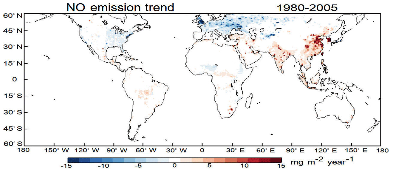
Figure 5Trends in MERRA-2 GMI NO emissions (units mg m −2 yr−1) for 1980–2005. This figure is similar to Fig. 2, except for having an earlier 1980–2005 time record.
As with OMI/MLS and GMI TCO trends in Fig. 1 there are discrepancies between the TOMS and model TCO trends in Fig. 4. For TOMS TCO in Fig. 4 there are regions of negative trends (in blue) of as much as −0.6 DU decade−1 over ocean in both hemispheres that are not explainable. Trends for GMI in Fig. 4 are instead largely positive within these regions and actually positive throughout much of the SH when compared with TOMS. This suggests that the TOMS trends may be biased slightly low overall, provided that the simulation is closer to truth.
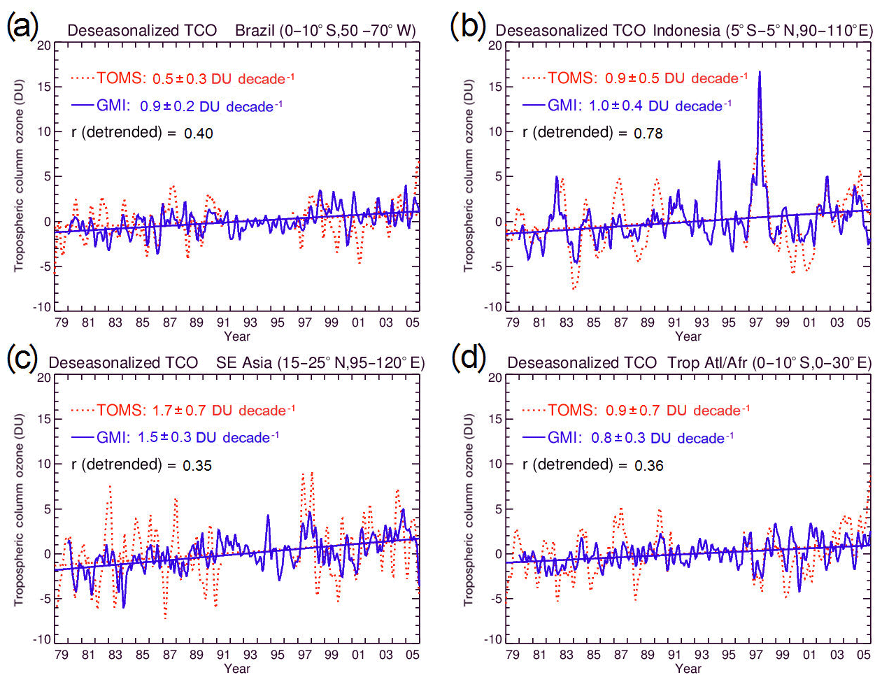
Figure 6(a) Deseasonalized TCO for TOMS (red, dashed curve) and the MERRA-2 GMI model (blue, solid curve) for Brazil. Included are their MLR linear trends and calculated 2σ values (both in DU decade−1) averaged over the specified region. Shown also is the cross-correlation r between the two time series after removing their linear trends. (b) Same as (a), but for Indonesia. (c) Same as (a), but for SE Asia. (d) Same as (a), but for tropical Atlantic/Africa.
The trends for GMI TCO are positive over Brazil whereas OMI/MLS TCO shows only a hint of positive trends. It is likely that there will be smaller trends for TOMS because most ozone produced from biomass burning over Brazil lies in the lower troposphere, and also that TOMS has reduced the ability to detect ozone in the lower troposphere. The GMI simulation shows that of the DU decade−1 TCO trend over Brazil in Fig. 4, about +0.9 DU decade−1 of this trend comes from ozone in the lower troposphere below 500 hPa. With a known retrieval efficiency of 50 %–60 % below 500 hPa (and essentially 100 % above 500 hPa) for TOMS over Brazil, the model suggests that TOMS should detect a trend of about +0.5 DU decade−1 below 500 hPa. Therefore TOMS would then have a trend in TCO of about +0.9 DU decade−1, which is comparable to the DU decade−1 measured for TOMS in Fig. 4.
Trends in NO emissions during 1980–2005 for the GMI simulation are shown in Fig. 5. Figure 5 is similar to Fig. 2 except for an earlier time period coinciding with the TOMS record. The largest increases in tropospheric NO emissions in Fig. 5 are located over India and East and Southeast Asia, as noted earlier for Fig. 2. Negative trends over the eastern US are much less pronounced (nearly nonexistent) in Fig. 5 during the TOMS record compared to the negative trends for the region in Fig. 2.
In Fig. 6 we show some examples of time series of TCO for TOMS and MERRA-2 GMI in regions where both records exhibit statistically significant positive trends. The positive correlations between TOMS and model TCO in Fig. 6 are generally small compared to the correlations between OMI/MLS and model TCO in Fig. 3. The only large correlation in Fig. 6 is over Indonesia and is due to the intense El Niño of 1997–1998 that caused record increases in TCO in October 1997 in the region due to record levels of biomass burning (e.g., Chandra et al., 2003). The cross-correlations in the other panels in Fig. 6 are small; these smaller correlations indicate the noisy nature of TOMS measurements compared to OMI/MLS and also possibly larger uncertainties present in meteorological winds, temperatures, and emissions during these earlier TOMS years for the GMI simulation. Changes in the observing system increases transport uncertainties for MERRA-2; these transport uncertainties increase the further back we go in time with MERRA-2, in particular the TOMS record. The recent Aura period for MERRA-2 has both more observations and higher vertical resolution than during the TOMS record. Stauffer et al. (2019) suggests that there is less impact of the changing observing system using the “Replay” technique compared to traditional CTMs. Wargan et al. (2018) discusses changes in the observing system for MERRA-2 for 1998–2016, including changes in the input-assimilated radiances.
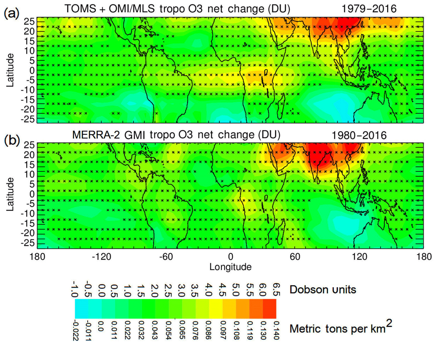
Figure 7(a) Net changes in TOMS and OMI/MLS TCO calculated for their combined time records (1979–2016). The net changes for TCO are shown in the color bar in both DU and metric tons of ozone per km2 (1 DU ≡0.0214 t km−2 for ozone). Asterisks denote grid points where net changes are statistically significant at the 2σ noise level. (b) Similar to (a), but for GMI TCO and years 1980–2016. Net change for GMI TCO is determined similar to the satellite measurements by adding together the net changes for the two records (i.e., for GMI, the 1980–2005 and 2005–2016 periods).
A main result from Figs. 4 and 6 is that the positive trends for both TOMS and MERRA-2 GMI TCO are substantially larger, by a factor of about 2 or more, during the OMI/MLS record compared to the TOMS record. The GMI simulation suggests that larger trends during the Aura record are the manifestation of an escalation of anthropogenic emissions and transport.
3.3 The merged record (1979–2016)
The net increases in tropospheric ozone over India and East and Southeast Asia for the merged 38-year record are sizable. Total changes in GMI and satellite-measured TCO for the merged record are shown in Fig. 7 where contour values were determined by adding changes from the individual TOMS and OMI/MLS records together. There are two regions of greatest increase in TCO in Fig. 7 for both GMI and the satellite measurements, one coinciding with the Near East to East Asia (increases of to +7 DU, or about 15 %–20 % average background ozone) and the other being tropical Africa and the Atlantic (increases of to +5 DU, with about 10 %–15 % average background ozone). There is also an area of negative net change in the SH lying between Australia and the maritime continent in Fig. 7 for both GMI and measurements (shown in blue); these negative variations over the SH Indian Ocean appear small and are not statistically significant.
The color bar in Fig. 7 also provides conversion from DU to tropospheric ozone mass surface density in units of metric tons per square kilometer. This conversion was included primarily to compare our results with the model simulation of Zhang et al. (2016). The large TCO trends over India and East and Southeast Asia in Fig. 7 are about +0.13 to +0.15 t km−2 for both GMI and the satellite data. These numbers are comparable to increases of t km−2 for this region as modeled by Zhang et al. (2016) for the years 1980–2010.
Using the 38-year net changes from the two independent regression analyses of TOMS+OMI/MLS TCO we can estimate the mass of ozone in the bands 0–30∘ N and 0–30∘ S for the years 1979 and 2016 that model simulations can compare with. Based on 2016 OMI/MLS TCO fields and extrapolated backwards linearly in time, mean area-weighted 0–30∘ N ozone masses are about 75.1 Tg for the year 1979 and 83.1 Tg for the year 2016, yielding about a 8.0±4.6 (2σ) Tg net increase. For 0–30∘ S, the mean numbers are 73.7 Tg for 1979 and 78.2 Tg for 2016, yielding about a 4.4±4.2 (2σ) Tg net increase. Changes in the tropospheric ozone mass in the 0–30∘ N band increased by about 10.1 %, and about 5.8 % for 0–30∘ S from 1979 to 2016 from the satellite measurements.
Figure 8 shows TCO time series from the merged satellite measurements for 1979–2016 centered over the two regions of largest increase in Fig. 7 (i.e., eastern Asia and equatorial Africa). In Fig. 8a and b TOMS is the solid red curve and OMI/MLS is the dotted blue curve. For plotting purposes, offsets were applied to the TOMS data in both panels using 2005 overlap measurements (see figure and caption). The last 5 years in both panels in Fig. 8 show that current OMPS TCO (solid black curves) with several years of overlap with OMI/MLS TCO will be useful to continue the OMI/MLS record which has already extended past 13 years.
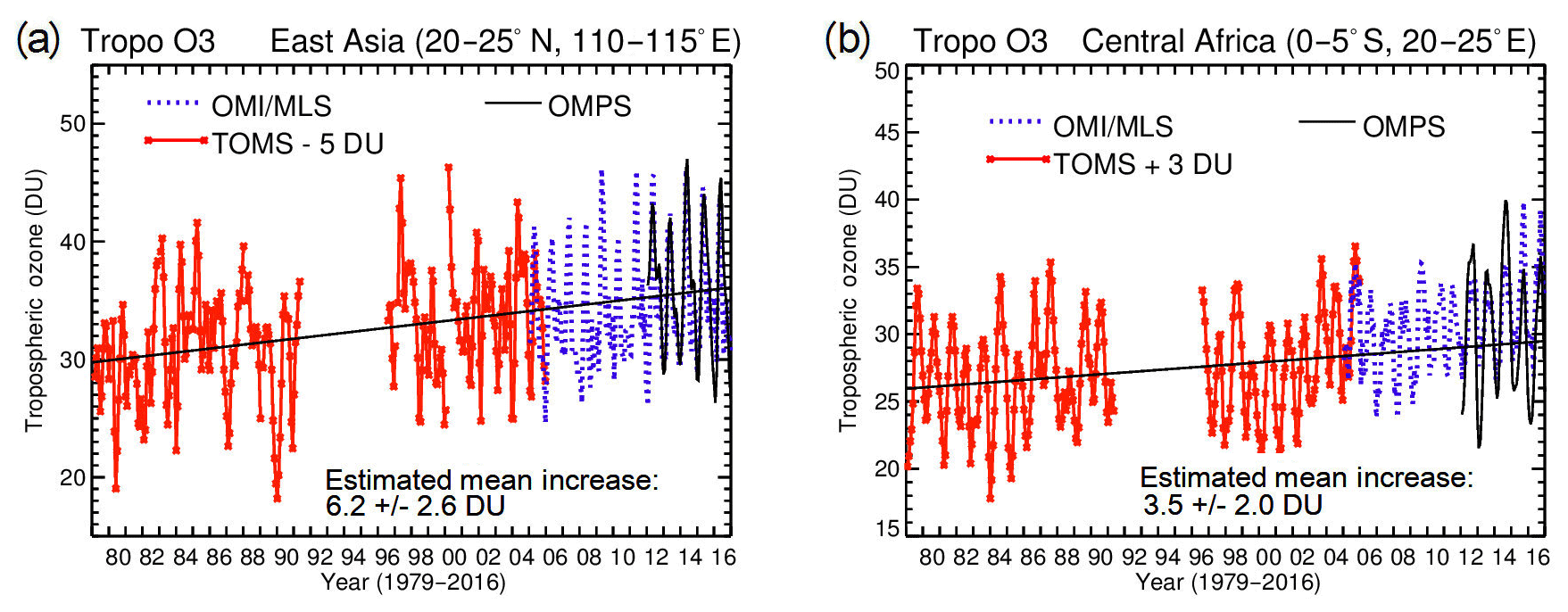
Figure 8(a) Merged time series of TOMS/OMI/MLS/OMPS TCO for 1979–2016 over East Asia centered at 22.5∘ N and 112.5∘ E ( region). The solid red curve is TOMS TCO and dashed blue curve is OMI/MLS. OMPS TCO (solid black curve) is also over-plotted with OMI/MLS TCO starting with 2012 for comparison. A constant adjustment of about −5 DU (using year 2005 coincident overlap data) was applied to the TOMS measurements for plotting with OMI/MLS. Both OMI/MLS and OMPS TCO also included offsets of +2 and −2 DU following comparisons with ozonesonde measurements (see Supplement). The indicated total increase of 6.2 DU was estimated using a regression best-fit line (black line shown) to the TOMS/OMI/MLS merged time series and agrees well with the 6–7 DU net increase for this region in Fig. 7. (b) Similar to (a) except for central Africa centered at 2.5∘ S, 22.5∘ E and a TOMS offset of +3 DU. The line-fit increase is slightly smaller than the 4–5 DU in Fig. 7. The estimated mean increases in both panels include calculated 2σ uncertainties.
Studies suggest that ozone in the lower stratosphere in both hemispheres has been decreasing over the last 1–2 decades despite the decrease in global CFC concentrations following the 1987 Montreal Protocol. Ball et al. (2018) evaluated global ozone trends for 1985–2016 by combining models with measurements from several satellite instruments. A conjecture as stated by Ball et al. (2018) is that while ozone in the upper stratosphere above ∼10 hPa appears to be recovering, ozone in the lower stratosphere appears to be decreasing, which models do not seem to replicate despite the decrease in CFCs. A main point of Ball et al. (2018) is that total ozone has not changed because the ongoing stratospheric ozone decrease is opposed by tropospheric ozone increase. A global decrease in lower stratospheric ozone of about 2 DU below 32 hPa was detected by Ball et al. (2018) and it appeared to be compensated largely by opposite increases in tropospheric ozone. In their study they included OMI/MLS TCO for 2005–2016 (i.e., their Figs. 4 and S13) and measured a trend in 60∘ S–60∘ N TCO of about +1.7 DU decade−1, which mostly cancels out the negative trend in stratospheric ozone. Wargan et al. (2018) in a related paper evaluated MERRA-2 assimilated ozone for 1998–2016 using an idealized atmospheric tracer also driven from MERRA-2 meteorological fields. Similar to Ball et al. (2018), Wargan et al. (2018) also found a net decrease in ozone in the lower stratosphere (i.e., within a 10 km layer above the tropopause) in both hemispheres; their trend values were about −1.2 DU decade−1 in the SH and about −1.7 DU decade−1 in the NH. Wargan et al. (2018) found evidence that these negative trends over the last two decades have been driven by enhanced isentropic transport of ozone between the tropical and extratropical lower stratosphere.
The increases in measured TCO from TOMS and OMI/MLS as indicated in Figs. 1, 3, 4 and 6–8 can have implications for evaluating global ozone trends, particularly for trends in total column ozone and assessment of the recovery of stratospheric ozone. One should be careful using total ozone to infer stratosphere ozone recovery if trends in TCO are not accounted for. The increases in TCO of +6 to +7 DU in Figs. 7–8 for India and eastern Asia represent a sizeable change even for total column ozone.
Studies suggest that ozone in the troposphere has increased globally throughout much of the 20th century due largely to increases in anthropogenic emissions. We provide evidence from combined satellite measurements and a chemical transport model that tropospheric ozone over the last four decades does indeed indicate increases that are global in nature, yet highly regional due to the combined effects of regional pollution and transport.
We have obtained tropospheric ozone trends for 1979–2016 by merging TOMS (1979–2005) and Aura OMI/MLS (2005–2016) satellite measurements. We included the MERRA-2 GMI CTM simulation to evaluate and possibly explain the global trend patterns found for both TOMS and OMI/MLS TCO. Trends were calculated independently for TOMS and OMI/MLS records using a linear regression model. Net changes in both measured and modeled TCO for the entire merged record were estimated by adding net changes for the TOMS and OMI/MLS time periods together.
A persistent trend pattern emerges with TCO for the GMI simulation and satellite measurements for both the TOMS and OMI/MLS records. The GMI model, and also measurements from TOMS and OMI/MLS all independently show large (positive) trends in TCO in the NH extending from the Near East to India and East and Southeast Asia, and further eastward over the Pacific Ocean. An important finding is that the trends in TCO for both the GMI model and satellite measurements for this region are smaller during the earlier part of the merged record; that is, the trends for both GMI and satellite measurements increase from about +1.2 to +1.4 DU decade−1 (1979–2005) to about +3 DU decade−1 or greater (2005–2016). Analysis of the NO emissions input to the GMI simulation indicates that the measured trends in tropospheric ozone in this region, including the escalation of increased trends during the latter Aura period, are consistent with increases in pollution in the region.
For the long merged record there are again strong similarities between the GMI simulation and satellite measurements of TCO. Net changes in tropospheric ozone for India and East and Southeast Asia for 1979–2016 are about +6 to +7 DU, or about 0.13–0.15 t km−2 for both the GMI and satellite TCO. These are pronounced increases in TCO representing ∼15 %–20 % average TCO background amounts. Both the GMI simulation and satellite measurements show that of these +6 to +7 DU increases over this broad area, about half or a slight majority of the change (i.e., DU) occurs during the Aura time record of 2005–2016. The GMI simulation and satellite measurements also depict a secondary maximum of TCO increase for 1979–2016 over the tropical Atlantic and African region of about +4 to +5 DU (∼10 %–15 % average background ozone).
Data used for this paper are publically accessible and can be found at http://acdb-ext.gsfc.nasa.gov/Data_services/ (last access: 7 March 2019).
The supplement related to this article is available online at: https://doi.org/10.5194/acp-19-3257-2019-supplement.
JRZ contributed as lead author to the production of the satellite tropospheric ozone measurements and analysis. LDO, SAS, ARD, and MAO were responsible for the production and analyses involving the MERRA-2 GMI simulation. RDM, PKB, GJL, DPH, NAK, SMF, LKH, GRJ, CJS, MTD and SLT all contributed to the paper by their involvement in the development of the satellite total ozone products including their long-term calibration necessary for ozone trend evaluation. LF contributed by his involvement in the MLS product development and use in this study. JCW and AMT provided key contributions to the paper regarding ozonesonde data and analysis.
The authors declare that they have no conflict of interest.
We thank the NASA Goddard Space Flight Center Ozone Processing Team for the
TOMS and OMI total ozone measurements and the Jet Propulsion Laboratory MLS
team for MLS v4.2 ozone. OMI is a Dutch–Finnish contribution to the Aura
mission. We thank WOUDC and the NDACC for providing extensive ozonesonde
measurements that we used for the comparisons and validation of satellite
tropospheric ozone. We also thank the NASA MAP program for supporting the
MERRA-2 GMI simulation and the NASA Center for Climate Simulation (NCCS) for
providing high-performance computing resources. Special thanks go to Ryan
Stauffer for important discussions regarding the ozonesonde measurements and
the MERRA-2 GMI simulation. More information on the MERRA-2 GMI simulation
and access is available at
https://acd-ext.gsfc.nasa.gov/Projects/GEOSCCM/MERRA2GMI/ (last access: 7 March 2019). Tropospheric ozone data used in this study are
available from the NASA Goddard Space Flight Center at
http://acdb-ext.gsfc.nasa.gov/Data_services/cloud_slice/ (last access: 7 March 2019) and links from the Aura Validation Data Center
(https://avdc.gsfc.nasa.gov/, last access: 7 March 2019). Funding for this research was provided in part by NASA
NNH14ZDA001N-DSCOVR.
Edited by: Michel Van
Roozendael
Reviewed by: two anonymous referees
Allen, D., Pickering, K., Duncan, B., and Damon, M.: Impact of lightning NO emissions on North American photochemistry as determined using the Global Modeling Initiative (GMI) model, J. Geophys. Res.-Atmos., 115, D22301, https://doi.org/10.1029/2010JD014062, 2010.
Anet, J. G., Steinbacher, M., Gallardo, L., Velásquez Álvarez, P. A., Emmenegger, L., and Buchmann, B.: Surface ozone in the Southern Hemisphere: 20 years of data from a site with a unique setting in El Tololo, Chile, Atmos. Chem. Phys., 17, 6477–6492, https://doi.org/10.5194/acp-17-6477-2017, 2017.
Ball, W. T., Alsing, J., Mortlock, D. J., Staehelin, J., Haigh, J. D., Peter, T., Tummon, F., Stübi, R., Stenke, A., Anderson, J., Bourassa, A., Davis, S. M., Degenstein, D., Frith, S., Froidevaux, L., Roth, C., Sofieva, V., Wang, R., Wild, J., Yu, P., Ziemke, J. R., and Rozanov, E. V.: Evidence for a continuous decline in lower stratospheric ozone offsetting ozone layer recovery, Atmos. Chem. Phys., 18, 1379–1394, https://doi.org/10.5194/acp-18-1379-2018, 2018.
Beig, G. and Singh, V.: Trends in tropical tropospheric column ozone from satellite data and MOZART model, Geophys. Res. Lett., 34, L17801, https://doi.org/10.1029/2007GL030460, 2007.
Cecil, D. J., Buechler, D. E., and Blakeslee, R. J.: Gridded lightning climatology fromTRMM-LIS and OTD: Dataset description, Atmos. Res., 135, 404–414, https://doi.org/10.1016/j.atmosres.2012.06.028, 2014.
Chandra, S., Ziemke, J. R., and Martin, R. V.: Tropospheric ozone at tropical and middle latitudes derived from TOMS/MLS residual: Comparison with a global model, J. Geophys. Res., 108, 4291, https://doi.org/10.1029/2002JD002912, 2003.
Cooper, O. R., Parrish, D. D., Ziemke, J. R., Balashov, N. V., Cupeiro, M., Galbally, I., Gilge, S., Horowitz, L., Jensen, N. R., Lamarque, J.-F., Naik, V., Oltmans, S. J., Schwab, J., Shindell, D. T., Thompson, A. M., Thouret, V., Wang, Y., and Zbinden, R. M.: Global distribution and trends of tropospheric ozone: An observation-based review, Elementa, 2, 000029, https://doi.org/10.12952/journal.elementa.000029, 2014.
Duncan, B. N., Martin, R. V., Staudt, A. C., Yevich, R., and Logan, J. A.: Interannual and seasonal variability of biomass burning emissions constrained by satellite observations, J. Geophys. Res.-Atmos., 108, 4100, https://doi.org/10.1029/2002jd002378, 2003.
Duncan, B. N., Strahan, S. E., Yoshida, Y., Steenrod, S. D., and Livesey, N.: Model study of the cross-tropopause transport of biomass burning pollution, Atmos. Chem. Phys., 7, 3713–3736, https://doi.org/10.5194/acp-7-3713-2007, 2007.
Gaudel, A., Cooper, O. R., Ancellet, G., Barret, B., Boynard, A., Burrows, J. P., Clerbaux, C., Coheur, P.-F., Cuesta, J., Cuevas, E., Doniki, S., Dufour, G., Ebojie, F., Foret, G., Garcia, O., Granados-Muñoz, M. J., Hannigan, J., Hase, F., Hassler, B., Huang, G., Hurtmans, D., Jaffe, D., Jones, N., Kalabokas, P., Kerridge, B., Kulawik, S., Latter, B., Leblanc, T., Le Flochmoën, E., Lin, W., Liu, J., Liu, X., Mahieu, E., McClure-Begley, A., Neu, J., Osman, M., Palm, M., Petetin, H., Petropavlovskikh, I., Querel, R., Rahpoe, N., Rozanov, A., Schultz, M. G., Schwab, J., Siddans, R., Smale, D., Steinbacher, M., Tanimoto, H., Tarasick, D., Thouret, V., Thompson, A. M., Trickl, T., Weatherhead, E., Wespes, C., Worden, H., Vigouroux, C., Xu, X., Zeng, G., and Ziemke, J.: Tropospheric Ozone Assessment Report: Present-day distribution and and trends of tropospheric ozone relevant to climate and global atmospheric chemistry model evaluation, Elementa, 6, p. 39, https://doi.org/10.1525/elementa.291, 2018.
Gelaro, R., McCarty, W., Suárez, M. J., Todling, R., Molod, A., Takacs, L., Randles, C. A., Darmenov, A., Bosilovich, M. G., Reichle, R., Wargan, K., Coy, L., Cullather, R., Draper, C., Akella, S., Buchard, V., Conaty, A., da Silva, A. M., Gu, W., Kim, G., Koster, R., Lucchesi, R., Merkova, D., Nielsen, J. E., Partyka, G., Pawson, S., Putman, W., Rienecker, M., Schubert, S. D., Sienkiewicz, M., and Zhao, B.: The Modern-Era Retrospective Analysis for Research and Applications, Version 2 (MERRA-2), J. Climate, 30, 5419–5454, https://doi.org/10.1175/JCLI-D-16-0758.1, 2017.
Giglio, L., Randerson, J., and van der Werf, G.: Analysis of daily, monthly, and annual burned area using the fourth-generation global fire emissions database (GFED4), J. Geophys. Res.-Biogeo., 118, 317–328, https://doi.org/10.1002/jgrg.20042, 2013.
Granier, C, Bessagnet, B., Bond, T., D'Angiola, A, Denier van der Gon, H., Frost, G. J., Heil, A., Kaiser, J. W., Kinne, S., Klimont, Z., Kloster, S., Lamarque, J.-F., Liousse, C., Masui, T., Meleux, F., Mieville, A., Ohara, T., Raut, J.-C., Riahi, K., Schultz, M. G., Smith, S. J., Thompson, A., van Aardenne, J., van der Werf, G. R., and van Vuuren, D. P.: Evolution of anthropogenic and biomass burning emissions of air pollutants at global and regional scales during the 1980–2010 period, Climatic Change, 109, 163–190, https://doi.org/10.1007/s10584-011-0154-1, 2011.
Guenther, A., Baugh, B., Brasseur, G., Greenberg, J., Harley, P., Klinger, L., Serça, D., and Vierling, L.: Isoprene emission estimates and uncertainties for the central African EXPRESSO study domain, J. Geophys. Res., 104, 30625–30639, https://doi.org/10.1029/1999JD900391, 1999.
Guenther, A., Geron, C., Perce, T., Lamb, B., Harley, P., and Fall, R.: Natural emissions of non-methane volatile organic compounds, carbon monoxide, and oxides of nitrogen from North America, Atmos. Environ. 34, 2205–2230, 2000.
Heue, K.-P., Coldewey-Egbers, M., Delcloo, A., Lerot, C., Loyola, D., Valks, P., and van Roozendael, M.: Trends of tropical tropospheric ozone from 20 years of European satellite measurements and perspectives for the Sentinel-5 Precursor, Atmos. Meas. Tech., 9, 5037–5051, https://doi.org/10.5194/amt-9-5037-2016, 2016.
Krotkov, N. A., McLinden, C. A., Li, C., Lamsal, L. N., Celarier, E. A., Marchenko, S. V., Swartz, W. H., Bucsela, E. J., Joiner, J., Duncan, B. N., Boersma, K. F., Veefkind, J. P., Levelt, P. F., Fioletov, V. E., Dickerson, R. R., He, H., Lu, Z., and Streets, D. G.: Aura OMI observations of regional SO2 and NO2 pollution changes from 2005 to 2015, Atmos. Chem. Phys., 16, 4605–4629, https://doi.org/10.5194/acp-16-4605-2016, 2016.
Lamarque, J.-F., Bond, T. C., Eyring, V., Granier, C., Heil, A., Klimont, Z., Lee, D., Liousse, C., Mieville, A., Owen, B., Schultz, M. G., Shindell, D., Smith, S. J., Stehfest, E., Van Aardenne, J., Cooper, O. R., Kainuma, M., Mahowald, N., McConnell, J. R., Naik, V., Riahi, K., and van Vuuren, D. P.: Historical (1850–2000) gridded anthropogenic and biomass burning emissions of reactive gases and aerosols: methodology and application, Atmos. Chem. Phys., 10, 7017–7039, https://doi.org/10.5194/acp-10-7017-2010, 2010.
Lee, H.-J., Kim, S.-W., Brioude, J., Cooper, O. R., Frost, G. J., Kim, C.-H., Park, R. J., Trainer, M., and Woo, J.-H.: Transport of NOx in East Asia identified by satellite and in-situ measurements and Lagrangian particle dispersion model simulations, J. Geophys. Res., 119, 2574–2596, https://doi.org/10.1002/2013JD021185, 2014.
Leventidou, E., Weber, M., Eichmann, K.-U., Burrows, J. P., Heue, K.-P., Thompson, A. M., and Johnson, B. J.: Harmonisation and trends of 20-year tropical tropospheric ozone data, Atmos. Chem. Phys., 18, 9189–9205, https://doi.org/10.5194/acp-18-9189-2018, 2018.
Lin, M., Horowitz, L. W., Payton, R., Fiore, A. M., and Tonnesen, G.: US surface ozone trends and extremes from 1980 to 2014: quantifying the roles of rising Asian emissions, domestic controls, wildfires, and climate, Atmos. Chem. Phys., 17, 2943–2970, https://doi.org/10.5194/acp-17-2943-2017, 2017.
Lu, X., Zhang, L., Zhao, Y., Jacob, D. J., Hu, Y., Hu, L., Gao, M., Liu, X., Petropavlovskikh, I., Mclure-Begley, A., and Quirel, R.: Surface and tropospheric ozone trends in the Southern Hemisphere since 1990: possible linkages to poleward expansion of the Hadley Circulation, Sci. Bull., 1–10, https://doi.org/10.1016/j.scib.2018.12.021, online first, 2018.
Molod, A., Takacs, L., Suarez, M., and Bacmeister, J.: Development of the GEOS-5 atmospheric general circulation model: evolution from MERRA to MERRA2, Geosci. Model Dev., 8, 1339–1356, https://doi.org/10.5194/gmd-8-1339-2015, 2015.
Nielsen, J. E., Pawson, S., Molod, A., Auer, B., da Silva, A. M., Douglass, A. R., Duncan, B., Liang, Q., Manyin, M., Oman, L. D., Putman, W., Strahan, S. E., and Wargan, K.: Chemical mechanisms and their applications in the Goddard Earth Observing System (GEOS) earth system model, J. Adv. Model. Earth Sy., 9, 3019–3044, https://doi.org/10.1002/2017MS001011, 2017.
Oman, L. D., Douglass, A. R., Ziemke, J. R., Rodriguez, J. M., Waugh, D. W., and Nielsen, J. E.: The ozone response to ENSO in Aura satellite measurements and a chemistry-climate simulation, J. Geophys. Res., 118, 965–976, https://doi.org/10.1029/2012JD018546, 2013.
Orbe, C., Oman, L. D., Strahan, S. E., Waugh, D. W., Pawson, S., Takacs, L. L., and Molod, A. M.: Large-Scale Atmospheric Transport in GEOS Replay Simulations, J. Adv. Model. Earth Sy., 9, 2545–2560, 2017.
Parrish, D. D., Law, K. S., Staehelin, J., Derwent, R., Cooper, O. R., Tanimoto, H., Volz-Thomas, H., Gilge, S., Scheel, H.-E., Steinbacher, M., and Chan, E.: Lower tropospheric ozone at northern mid-latitudes: Changing seasonal cycle, Geophys. Res. Lett., 40, 1631–1636, https://doi.org/10.1002/grl.50303, 2013.
Stauffer, R. M., Thompson, A. M., Oman, L. D., and Strahan, S. E.: The effects of a changing observing system on MERRA-2-based ozone profile simulations (1980–2016), J. Geophys. Res., in review, 2019.
Strode, S. A., Rodriguez, J. M., Logan, J. A., Cooper, O. R., Witte, J. C., Lamsal, L. N., Damon, M., Van Aartsen, B., Steenrod, S. D., and Strahan, S. E.: Trends and variability in surface ozone over the United States, J. Geophys. Res.-Atmos., 120, 9020–9042, https://doi.org/10.1002/2014JD022784, 2015.
Thompson, A. M., Witte, J. C., Sterling, C., Jordan, A., Johnson, B. J., Oltmans, S. J., Fujiwara, M., Vömel, H., Allaart, M., Piters, A., Coetzee, G. J. R., Posny, F., Corrales, E., Andres Diaz, J., Félix, C., Komala, N., Lai, N., Maata, M., Mani, F., Zainal, Z., Ogino, S.-Y., Paredes, F., Luiz Bezerra Penha, T., Raimundo da Silva, F., Sallons-Mitro, S., Selkirk, H. B., Schmidlin, F. J., Stuebi, R., and Thiongo, K.: First reprocessing of Southern Hemisphere Additional Ozonesondes (SHADOZ) Ozone Profiles (1998–2016). 2. Comparisons with satellites and ground-based instruments, J. Geophys. Res., 122, 13000–13025, https://doi.org/10.1002/2017JD027406, 2017.
Vasilkov, A., Joiner, J., Spurr, R., Bhartia, P. K., Levelt, P., and Stephens, G.: Evaluation of the OMI cloud pressures derived from rotational Raman scattering by comparisons with other satellite data and radiative transfer simulations, J. Geophys. Res., 113, D15S19, https://doi.org/10.1029/2007JD008689, 2008.
Wang, Y., Jacob, D. J., and Logan, J. A.: Global simulation of tropospheric O3-NOx-hydrocarbon chemistry: 1. Model formulation, J. Geophys. Res., 103, 10713–10725, https://doi.org/10.1029/98JD00158, 1998.
Wargan, K., Orbe, C., Pawson, S., Ziemke, J. R., Oman, L. D., Olsen, M. A., Coy, L., and Knowland, K. E.: Recent decline in lower stratospheric ozone attributed to circulation changes, Geophys. Res. Lett., 45, 5166–5176, https://doi.org/10.1029/2018GL077406, 2018.
Weatherhead, E. C., Reinsel, G. C., Tiao, G. C., Meng, X.-L., Choi, D., Cheang, W.-K., Keller, T., DeLuisi, J., Wuebbles, D. J., Kerr, J. B., Miller, A. J., Oltmans, S. J., and Frederick, J. E.: Factors affecting the detection of trends: Statistical considerations and applications to environmental data, 103,17149–17161, https://doi.org/10.1029/98JD00995, 1998.
Wesely, M. L. and Hicks, B. B.: Some factors that affect the deposition rates of sulfur dioxide and similar gases on vegetation, Japca J. Air Waste Ma., 27, https://doi.org/10.1080/00022470.1977.10470534, 1977.
Witte J. C., Thompson, A. M., Smit, H. G. J., Fujiwara, M., Posny, F., Coetzee, G. J. R., Northam, E. T., Johnson, B. J., Sterling, C. W., Mohammed, M., Ogino, S.-Y., Jordan, A., daSilva, F. R., and Zainal, Z.: First reprocessing of Southern Hemisphere ADditional OZonesondes (SHADOZ) profile records (1998–2015) 1: Methodology and evaluation, J. Geophys. Res., 122, 6611–6636, https://doi.org/10.1002/2016JD026403, 2017.
Witte, J. C., Thompson, A. M., Smit, H. G. J., Vömel, H., Posny, F., and Stuebi, R.: First reprocessing of Southern Hemisphere Additional Ozonesondes (SHADOZ) Profile Records. 3. Uncertainty in ozone profile and total column, J. Geophys. Res., 123, 3243–3268, https://doi.org/10.1002/2017JD027791, 2018.
World Meteorological Organization: Scientific assessment of ozone depletion: Global Ozone Research and Monitoring, Project-Report No. 55, 416 pp., Geneva, Switzerland, 2014.
Yienger, J. J. and Levy, H.: Empirical-model of global soil-biogenic NOx emissions, J. Geophys. Res.-Atmos., 100, 11447–11464, https://doi.org/10.1029/95jd00370, 1995.
Young, P. J., Archibald, A. T., Bowman, K. W., Lamarque, J.-F., Naik, V., Stevenson, D. S., Tilmes, S., Voulgarakis, A., Wild, O., Bergmann, D., Cameron-Smith, P., Cionni, I., Collins, W. J., Dalsøren, S. B., Doherty, R. M., Eyring, V., Faluvegi, G., Horowitz, L. W., Josse, B., Lee, Y. H., MacKenzie, I. A., Nagashima, T., Plummer, D. A., Righi, M., Rumbold, S. T., Skeie, R. B., Shindell, D. T., Strode, S. A., Sudo, K., Szopa, S., and Zeng, G.: Pre-industrial to end 21st century projections of tropospheric ozone from the Atmospheric Chemistry and Climate Model Intercomparison Project (ACCMIP), Atmos. Chem. Phys., 13, 2063–2090, https://doi.org/10.5194/acp-13-2063-2013, 2013.
Zhang, Y., Cooper, O. R., Gaudel, A., Thompson, A. M., Nedelec, P., Ogino, S.-Y., and West, J. J.: Tropospheric ozone change from 1980 to 2010 dominated by equatorward re-distribution of emissions, Nat. Geosci., 9, 875–879, https://doi.org/10.1038/NGEO2827, 2016.
Ziemke, J. R. and Chandra, S.: Development of a climate record of tropospheric and stratospheric column ozone from satellite remote sensing: evidence of an early recovery of global stratospheric ozone, Atmos. Chem. Phys., 12, 5737–5753, https://doi.org/10.5194/acp-12-5737-2012, 2012.
Ziemke, J. R., Chandra, S., McPeters, R. D., and Newman, P.: Dynamical proxies of column ozone with applications to global trend models, J. Geophys. Res., 102, 6117–6129, https://doi.org/10.1029/96JD03783, 1997.
Ziemke, J. R., Chandra, S., and Bhartia, P. K.: Two new methods for deriving tropospheric column ozone from TOMS measurements: The assimilated UARS MLS/HALOE and convective-cloud differential techniques, J. Geophys. Res., 103, 22115–22127, 1998.
Ziemke, J. R., Chandra, S., and Bhartia, P. K.: A 25-year data record of atmospheric ozone from TOMS Cloud Slicing: Implications for trends in stratospheric and tropospheric ozone, J. Geophys. Res., 110, D15105, https://doi.org/10.1029/2004JD005687, 2005.
Ziemke, J. R., Chandra, S., Duncan, B. N., Froidevaux, L., Bhartia, P. K., Levelt, P. F., and Waters, J. W.: Tropospheric ozone determined from Aura OMI and MLS: Evaluation of measurements and comparison with the Global Modeling Initiative's Chemical Transport Model, J. Geophys. Res., 111, D19303, https://doi.org/10.1029/2006JD007089, 2006.