the Creative Commons Attribution 4.0 License.
the Creative Commons Attribution 4.0 License.
 | 07 Mar 2019
Characterizing uncertainties in atmospheric inversions of fossil fuel CO2 emissions in California
Heather Graven
Alistair J. Manning
Emily White
Tim Arnold
Marc L. Fischer
Seongeun Jeong
Xinguang Cui
Matthew Rigby
Atmospheric inverse modelling has become an increasingly useful tool for evaluating emissions of greenhouse gases including methane, nitrous oxide, and synthetic gases such as hydrofluorocarbons (HFCs). Atmospheric inversions for emissions of CO2 from fossil fuel combustion (ffCO2) are currently being developed. The aim of this paper is to investigate potential errors and uncertainties related to the spatial and temporal prior representation of emissions and modelled atmospheric transport for the inversion of ffCO2 emissions in the US state of California. We perform simulation experiments based on a network of ground-based observations of CO2 concentration and radiocarbon in CO2 (a tracer of ffCO2), combining prior (bottom-up) emission models and transport models currently used in many atmospheric studies. The potential effect of errors in the spatial and temporal distribution of prior emission estimates is investigated in experiments by using perturbed versions of the emission estimates used to create the pseudo-data. The potential effect of transport error was investigated by using three different atmospheric transport models for the prior and pseudo-data simulations. We find that the magnitude of biases in posterior total state emissions arising from errors in the spatial and temporal distribution in prior emissions in these experiments are 1 %–15 % of posterior total state emissions and are generally smaller than the 2σ uncertainty in posterior emissions. Transport error in these experiments introduces biases of −10 % to +6 % into posterior total state emissions. Our results indicate that uncertainties in posterior total state ffCO2 estimates arising from the choice of prior emissions or atmospheric transport model are on the order of 15 % or less for the ground-based network in California we consider. We highlight the need for temporal variations to be included in prior emissions and for continuing efforts to evaluate and improve the representation of atmospheric transport for regional ffCO2 inversions.
- Article
(4584 KB) - Full-text XML
-
Supplement
(861 KB) - BibTeX
- EndNote


The US state of California currently emits roughly 100 Tg C of fossil fuel CO2 (ffCO2) each year (CARB, 2018), or approximately 1 % of global emissions (Boden et al., 2017). The passing of California's “Global Warming Solutions Act” (AB-32) in 2006 requires that overall greenhouse gas emissions in California be reduced to their 1990 levels by 2020 (a 15 % reduction compared to business-as-usual emissions), with further reductions of 40 % below 1990 levels planned for 2030 and 80 % below 1990 levels by 2050. The California Air Resources Board (CARB) is responsible for developing and maintaining a “bottom-up” inventory of greenhouse gas emissions to verify these reduction targets. However, previous studies have shown that such inventories may have errors or incomplete knowledge of sources (e.g. Marland et al., 1999; Andres et al., 2012). Uncertainties in inventories of annual ffCO2 emissions from most developed countries (i.e. UNFCCC Annex I and Annex II) have been estimated to be between 5 %–10 % (Andres et al., 2012), and uncertainties can become much larger at subnational levels (Hogue et al., 2016). In a recent study Fischer et al. (2017) found that discrepancies between bottom-up gridded inventories of ffCO2 emissions were 11 % of California's total state emissions.
Previous research has shown that inferring ffCO2 emissions from atmospheric measurements, including measurements of ffCO2 tracers, could provide independent emission estimates on urban to continental scales (e.g. Basu et al., 2016; Lauvaux et al., 2016; Fischer et al., 2017; Graven et al., 2018). Such estimates are derived from observations through the use of an atmospheric chemical transport model and a suitable inverse method in a process often referred to as “inverse modelling” or an “inversion”. Distinguishing enhancements of CO2 due to anthropogenic or biogenic sources can be done using measurements of radiocarbon in CO2 (Δ14CO2), since CO2 emitted from fossil fuel combustion is devoid of 14CO2 due to radioactive decay (Levin et al., 2003).
Recent studies with both real atmospheric measurements of Δ14CO2 and with observing system simulation experiments (OSSEs) at a network of sites have shown that atmospheric Δ14CO2 can be used to estimate monthly mean Californian ffCO2 emissions with posterior uncertainties of 5 %–8 %, levels that are useful for the evaluation of bottom-up ffCO2 emission estimates. Furthermore, Graven et al. (2018) found that their posterior emission estimates were not significantly different from the California Air Resources Board's reported ffCO2 emissions, providing tentative validation of California's reported ffCO2 emissions in 2014 and 2015. In another study using aircraft-based Δ14CO2 measurements, Turnbull et al. (2011) found that ffCO2 emissions from Sacramento County in February 2009 had a mean difference of −17 %, ranging from −43 % to +133 % with the Vulcan emission estimate (Gurney et al., 2009).
Although atmospheric inversions may provide a method for estimating emissions that is useful for evaluating emission reduction policies, such as AB-32, systematic errors can arise from the atmospheric transport and prior emission models (e.g. Nassar et al., 2014; Liu et al., 2014; Hungershoefer et al., 2010; Chevallier et al., 2009, Gerbig et al., 2003). Comparisons of CO2 simulated by different transport models have been conducted globally (e.g. Gurney et al., 2003; Peylin et al., 2013) and on the European continental scale (Peylin et al., 2011). The latter found that transport model error resulted in differences in modelled ffCO2 concentrations that were 2–3 times larger than using the same transport model but different prior emissions, depending on the location and time of year. However, comparisons of ffCO2 simulated by different high-resolution models (25 km or less) at regional scales are still lacking.
The objective of this paper is to examine the sensitivity of a regional inversion for Californian ffCO2 emissions to errors in the prior emission estimate and transport model. We build on previous work by Fischer et al. (2017) that developed an observation system simulation experiment to estimate the uncertainties in both California statewide ffCO2 emissions and biospheric fluxes that might be obtained using an atmospheric inversion. Their inversion was driven by a combination of in situ tower measurements; satellite column measurements from NASA's Orbiting Carbon Observatory (OCO-2); prior flux estimates; a regional atmospheric transport modelling system; and estimated uncertainties in prior CO2 flux models, ffCO2 measurements using radiocarbon, OCO-2 measurements, and atmospheric transport. In contrast to Fischer et al. (2017) we focus only on ffCO2 emissions and use a network of flask samples without incorporating satellite measurements.
Our approach is to use simulation experiments to quantify representation and transport error using the inversion set-up and the observation network from Graven et al. (2018) as a test case. Specifically we test whether the inversion can estimate the “true” emissions that were used to produce the pseudo-data within the uncertainties when the prior emission estimate includes spatial and temporal representation errors within the scope of current emission estimates (Vulcan v2.2 and EDGAR v4.2 FT2010). We further test whether the inversion can estimate true emissions within the uncertainties when the transport model used for the prior simulation is different from the transport model used to produce the pseudo-data, emulating transport error.
The analysis approach applies a Bayesian inversion developed from previous work that combines atmospheric observations, atmospheric transport modelling, prior flux models, and an uncertainty specification (Jeong et al., 2013; Fischer et al., 2017). Here, the inversion scale's prior emission estimates for 15 regions (Fig. 1a, Table 1) termed “air basins”, classified by the California Air Resources Board for air-quality control (https://www.arb.ca.gov/desig/adm/basincnty.htm, last access: 1 March 2019).
Table 1The 15 air basins of California with respective emissions as estimated by Vulcan and EDGAR models. Also shown are the SD prior uncertainty estimate (Fischer et al., 2017) and difference in magnitude between Vulcan and EDGAR for each air basin. Air basin numbers correspond to those marked in Fig. 1.

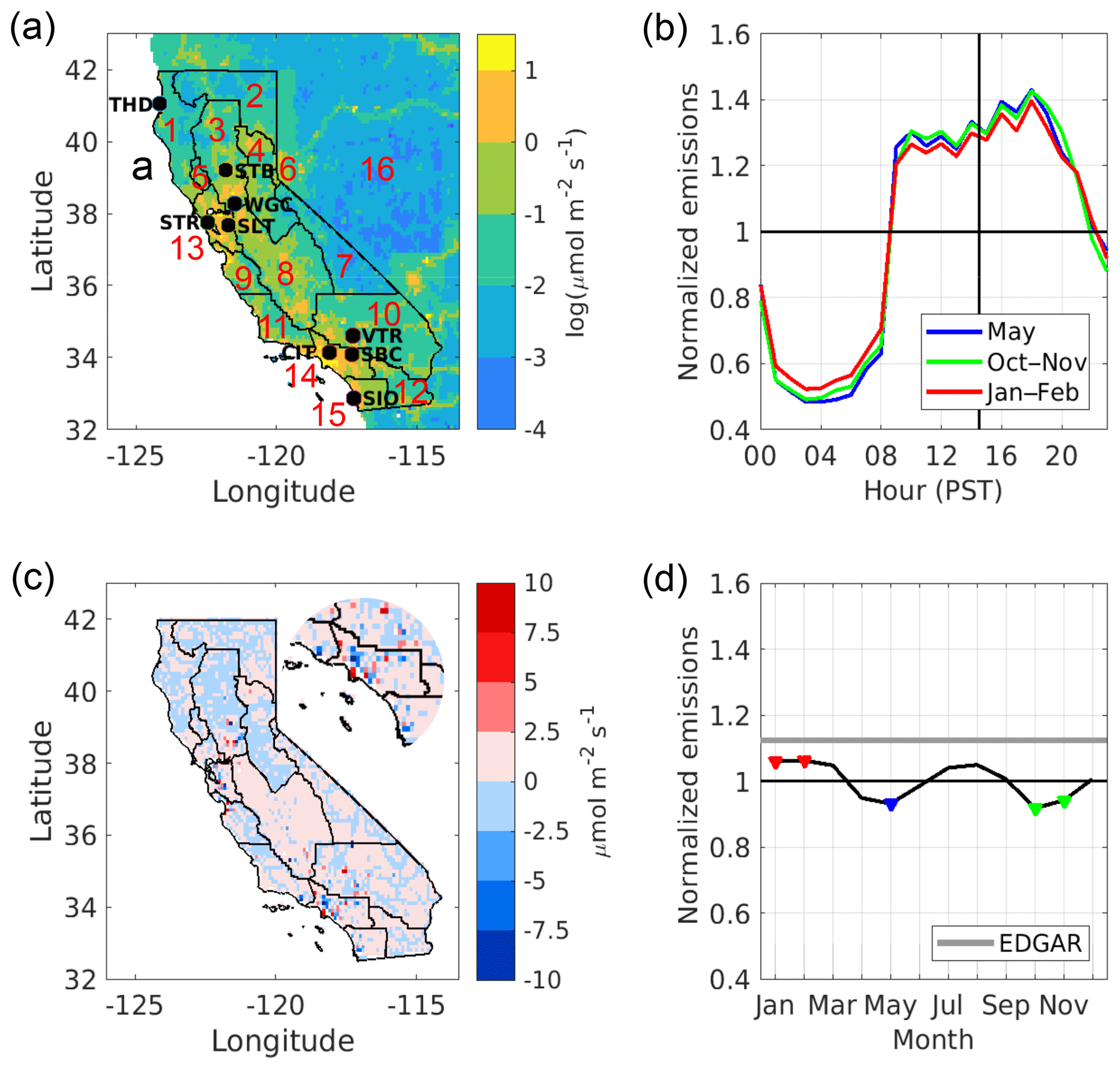
Figure 1(a) The location of the nine tower sites in the observation network (marked with black circles): Trinidad Head (THD), Sutter Buttes (STB), Walnut Grove (WGC), Sutro Tower (STR), Sandia – Livermore (LVR), Victorville (VTR), San Bernardino (SBC), Caltech (CIT), and Scripps Institute of Oceanography (SIO). The 15 air basins are marked with black lines, with region 16 representing emissions from outside California within the model domain. Underlaid is a map of annual mean ffCO2 emissions from the Vulcan v2.2 emission map within the United States and EDGAR v4.2 (FT2010) for emission from outside the US. (b) Vulcan diurnal emissions normalized to campaign-averaged emissions for the three campaigns; (c) scaled EDGAR emissions subtracted from Vulcan emissions map, where EDGAR has been scaled to have the same air basin total emissions. The inset shows an enlarged view of southwestern California. (d) Average monthly emissions normalized to Vulcan annual emissions. Shown in both (b) and (d) are EDGAR annual invariant emissions (grey).
2.1 Observation network
As a test case for exploring uncertainties in ffCO2 inversions, we use the observation network of nine tower sites in California that was used to collect flask samples for measurements of CO2 and radiocarbon in CO2 in 2014 and 2015 and simulate the same campaign periods (Fig. 1a; Graven et al., 2018). Three month-long campaigns were conducted: 1–29 May 2014, 15 October–14 November 2014, and 26 January–15 February 2015, with flasks sampled approximately every 2–3 days at 22:30 GMT (14:30 LST – local standard time). We replicate the sample availability in Graven et al. (2018), including the reduction in observation sites used in January–February 2015. The time of observation chosen as the planetary boundary layer is usually deepest in the afternoon so that errors in the modelled boundary layer concentration are considered smaller (Jeong et al., 2013), and afternoon concentrations are more representative of large regions.
The observed ffCO2 concentration at a given site can be calculated by (Levin et al., 2003; Turnbull et al., 2009)
where Cobs is the total observed CO2 concentration at a given site. Δ refers to Δ14C, the ratio of 14C ∕ C reported in part per thousand deviation from a standard ratio, including corrections for mass-dependent isotopic fractionation and sample age (Stuiver and Polach, 1977). Δbg, Δobs, and Δff are the Δ14CO2 of background, observed, and fossil fuel CO2, respectively, where Δff is −1000 ‰, since ffCO2 is devoid of 14CO2. The term β is a correction for the effect of other influences on Δ14CO2, principally heterotrophic respiration (Turnbull et al., 2009). In the experiments we present here, we do not explicitly calculate Δ14CO2 or the other terms in Eq. (1), rather we simulate ffCO2 and specify its uncertainty to be the same as the uncertainty in radiocarbon-based estimates of ffCO2. Following Fischer et al. (2017), total observational uncertainty for ffCO2 was assumed to be 1.5 ppm (1σ), encapsulating measurement uncertainty, background uncertainty, and uncertainty in β. This is consistent with Graven et al. (2018), who estimated total uncertainty in ffCO2 for individual samples of 1.0 to 1.9 ppm.
2.2 Prior emission estimates and prior uncertainty
The two prior emission estimates used here are gridded products produced by EDGAR (version FT2010; EDGAR, 2011) for the year 2008 and Vulcan (version 2.2) for 2002 (Gurney et al., 2009). EDGAR is produced at an annual resolution, whilst Vulcan has an hourly resolution. The two models use different emission data and different methods to spatially allocate emissions with annually averaged statewide emissions differing by 17.8 Tg C (∼19 % of mean emissions) and up to 11.6 Tg C for individual air basins in California (Table 1). Although our campaigns took place in 2014–2015, we use emission estimates from Vulcan for the year 2002 and EDGAR for 2008, as emission estimates are not available from Vulcan and EDGAR for 2014–2015. The difference in total state emissions between 2002, 2008, and 2014–2015 is 3–6 Tg C (CARB, 2018), much less than the EDGAR–Vulcan difference of 17.8 Tg C.
We estimate prior uncertainty in the same way as in Fischer et al. (2017), using a comparison of four gridded emission estimates in California (Vulcan version 2.2, EDGAR FT2010, ODIAC version 2013, and FFDAS version 2) as well as a comparison across an ensemble of emission estimates for one model (FFDAS version 2; Asefi-Najafabady et al., 2014). Prior uncertainty is specified for the whole air basin. The relative 1σ standard deviation across the four inventories is between 8 % and 100 % for individual air basins (Table 1), and this is what we use to specify the 1σ uncertainty in the prior emissions from each air basin. This estimate of prior uncertainty is referred to as “SD prior uncertainty”. We also conduct tests with an alternative prior uncertainty of 70 % for each air basin (referred to as “70 % prior uncertainty”). This was done to test the sensitivity of our results to the choice of prior uncertainty. Emissions occurring outside California were assumed to have an uncertainty of 100 % for both cases.
Table 2Comparison of the three atmospheric transport models used in this study.

2.3 Atmospheric transport models
We simulate ffCO2 using three different atmospheric transport models outlined in Table 2. These models are commonly used in regional atmospheric transport modelling and greenhouse gas inversion studies but to date have not been compared in California. Two of the transport models use different versions and parameterizations of the Weather Research and Forecast (WRF) model combined with the stochastic time-inverted Lagrangian transport (STILT) model. The third transport model uses meteorology from the UK Met Office's Unified Model (UM) combined with the Numerical Atmospheric-dispersion Modelling Environment (NAME).
The first WRF-STILT model is run at Lawrence Berkeley National Laboratory (WS-LBL; Fischer et al., 2017; Jeong et al., 2016; Bagley et al., 2017) and uses WRF version 3.5.1 (Lin et al., 2003; Nehrkorn et al., 2010). Estimates for the planetary boundary layer height (PBLH) are based on the Mellor–Yamada–Nakanishi–Niino version 2 (MYNN2) parameterization (Nakanishi and Niino, 2004, 2006). As in Jeong et al. (2016), Fischer et al. (2017) and Bagley et al. (2017), two land surface models (LSMs) are used depending on the location of the observation site. A five-layer thermal diffusion land surface model is used in the Central Valley for the May campaign, whilst the Noah LSM (Chen and Dudhia, 2001) is used in the remaining campaigns and regions of California. We implement multiple nested domains, with the outermost domain spanning 16–59∘ N and 154–137∘ W with a 36 km resolution, a second domain of 12 km resolution over western North America, and a third domain of 4 km resolution over California. Two urban domains of 1.3 km resolution are used in the San Francisco Bay area and the metropolitan area of Los Angeles. Footprints describing the sensitivity of an observation to surface emissions are calculated by simulating 500 model particles and tracking them backward for 7 days. The footprint of a given site and observation time is produced hourly for particles below 0.5 times the PBLH.
The second WRF-STILT model is from the CarbonTracker-Lagrange (WS-CTL), an effort led by the NOAA to produce standard footprints for greenhouse gas observation sites in North America (https://www.esrl.noaa.gov/gmd/ccgg/carbontracker-lagrange, last access: 1 March 2019). WS-CTL uses WRF version 2.1.2 and the Yonsei University (YSU; Hong et al., 2006) PBLH scheme coupled with the Noah land surface model and the MM5 (fifth-generation Pennsylvania State University National Center for Atmospheric Research mesoscale model; Grell et al., 1994) similarity theory-based surface layer scheme. As with WS-LBL, simulations are run for 7 days, and particles below 0.5 times the PBLH are used in the calculation of the footprint. Footprints have a spatial resolution of 0.1∘ for the first 24 h and 1∘ for the remaining 6 days. Footprints are disaggregated hourly for the first 24 h and then aggregated for the remaining 6 days. This approach captures the influence of temporally varying emissions that can be significant in the first 24 h but we assume to be negligible for the period longer than 24 h back in time. The 0.1∘ spatial resolution domain is 31∘ longitude by 21∘ latitude, with the domain centred on the release location. The 1∘ resolution has a domain of 170 to 50∘ E longitude and 10 to 80∘ N latitude. The WRF domain covers most of continental North America (Fig. 1 in Nehrkorn et al., 2010) with 30 km resolution and has a finer nest with 10 km spatial resolution over the continental US. WS-CTL simulates footprints for 500 particles released over a 2 h period between 21:00 and 23:00 GMT (Greenwich Mean Time; 13:00 and 15:00 PST – Pacific Standard Time). An exception is at Sutro Tower (STR), where footprints are only available for an instantaneous release of 500 particles at 22:10 GMT. Walnut Grove (WGC) footprints are available only for a release height of 30 m a.g.l., which is lower than the sampling height of 91 m a.g.l. used in the observation campaign (Graven et al., 2018) and used in the other two transport models. Footprints were available for 2014 but not for 2015, so the WS-CTL model is used for simulations of the May and October–November 2014 campaigns but not for the January–February 2015 campaign.
The third model, UM-NAME, is the UK Met Office's NAME model, version 3.6.5 (Jones et al., 2007), driven by meteorology from the Met Office's global numerical weather prediction model, the UM (Cullen, 1993). The UM has a horizontal resolution of ∼25 km up to July 2014, covering the period of the May 2014 campaign. The horizontal resolution was then increased to ∼17 km covering both the October–November 2014 and January–February 2015 campaigns. The temporal resolution of the UM meteorology is every 3 h for all campaigns. Following a similar approach to the WRF-STILT models, 500 particles were released instantaneously at 22:30 GMT and were simulated for hourly disaggregated footprints for the first 24 h and aggregated for the remaining 6 days. The footprints are calculated for the same horizontal resolution as the UM meteorology (25 or 17 km), where the particles present in the layer between 0 and 100 m a.g.l. are used to calculate the footprint. The computational domain covers 175.0 to 75∘ W longitude and 6.0 to 74∘ N latitude.
Simulated ffCO2 signals (the enhancement of CO2 concentration due to ffCO2 emissions within the model domain) are calculated by taking the product of the footprint and an emission estimate, both with the spatial resolution of the footprint at the native footprint resolution. The resulting concentration is summed for individual air basins. Following previous work, we assume a transport model uncertainty of 0.5 times the mean monthly signal in the pseudo-observations at each site (referred to as the “uncertainty parameter”; Jeong et al., 2013; Fischer et al., 2017). We also test the effect of changing the uncertainty parameter to 0.3 and 0.8. Ten ensembles were run for UM-NAME to test the effect of random errors on the calculation of the footprint. The RMSE was within 10 % of the mean monthly signal for most observation sites. This is similar to the findings of Jeong et al. (2012a), which the transport model uncertainty is based on. Two observation sites (Trinidad Head – THD, and Victorville – VTR) had a slightly higher RMSE, but both were within 20 % of the mean monthly signal.
2.4 Inversion method
Our inversion method is a Bayesian synthesis inversion to scale emissions in separate regions of California. We follow the same approach as Fischer et al. (2017) to solve for a vector of scaling factors, λ, for 15 air basins and a 16th region representing the area outside of California. Unlike Fischer et al. (2017), we do not split the San Joaquin Valley into two regions. The inversion uses the set of observations, c, and the matrix of predicted ffCO2 signals from each air basin, K, to optimize the cost function J:
λprior is the prior estimate of the scaling factors (a vector of those with length equal to the number of regions), and R and Qλ are the error covariance matrices relating to observational and model transport errors and prior emission estimate errors respectively. The non-diagonal elements of R and Qλ are zero, assuming uncorrelated errors in the prior emissions in each air basin and in the model and observations. This assumption for R is robust, as we only generate one pseudo-observation every 2–3 days. Included in R are observational errors and transport model errors, added in quadrature. Therefore if the average signal at an observation site is very small, then observational uncertainty (1.5 ppm) will dominate R. Minimizing J using the standard least-squares formulation under the assumption of Gaussian-distributed uncertainties gives the posterior estimate for λ as follows:
with the posterior error covariance given as
λpost and Vpost are computed separately for each of the three campaigns outlined in Sect. 2.1. Posterior emission estimates are the product of the λ post-emission and prior emission estimate from each air basin. Total state emissions are then calculated by summing the emissions in each air basin. Uncertainty in the statewide Californian posterior flux, including error correlations, is calculated as
where Eprior is a vector of ffCO2 emissions from each air basin.
2.5 Simulation experiments
We conduct a series of experiments to test the performance of the inversion in estimating the true emissions when the emission estimates or transport models used to produce pseudo-observations are different to those used to produce the prior simulations. The tests explore the effect differences in the magnitude, spatial distribution, and temporal variation of prior emissions have on posterior emissions. We also examine the effect of using different transport models to simulate pseudo-observations and to simulate prior concentrations.
As part of these experiments, we evaluate the impact of outlier removal on the simulation experiments. Outlier removal is generally used in atmospheric inversions when there is an issue with the ability of the model to simulate a particular observation. We use the outlier removal method outlined in Graven et al. (2018) and compare it with inversion results where no outliers are removed. In this outlier removal method, an observation (here, a pseudo-observation) is designated as an outlier if (1) the absolute difference between the ffCO2 signals in the observation and the prior simulation is greater than the average of the observed and simulated ffCO2 and (2) either the observed or simulated ffCO2 is greater than 5 ppm.
2.5.1 Difference in magnitude of emissions
First we test how well the inversion estimates the true emissions if the prior emissions have a systematic error in magnitude but have no error in the spatial or temporal distribution of emission and no error in atmospheric transport. In this experiment, the prior emission estimate is given by EDGAR, and the true ffCO2 signals were generated by scaling the EDGAR emissions in each air basin to match the annually averaged Vulcan emissions in that air basin. These differences range from 0.1 Tg C in San Diego to 11.6 Tg C in the San Joaquin Valley (Table 1). The EDGAR total state emissions are 12 % higher than the Vulcan emissions, so the bias in the prior estimate in the total state ffCO2 emissions is +12 %. The experiment is run for all the transport models with no temporal variation in emissions. This experiment assesses the performance of the inversion and the strength of the data constraint provided by the observation network in the simplest case, where the only errors in prior regional flux estimates are biases in their magnitudes. Prior uncertainty is fixed per air basin for all experiments.
2.5.2 Difference in spatial distribution of emissions
To investigate the bias in the posterior emission estimate that could result from errors in the spatial distribution of prior emissions within each air basin, we now use annually averaged Vulcan emissions as the true emissions and EDGAR emissions scaled in each air basin to match the annually averaged Vulcan emissions in that region as the prior estimate of emissions. In this experiment, the prior estimate of the total emissions in each air basin is unbiased, and we assess how differences in the spatial distribution of emissions between Vulcan and EDGAR in each air basin may lead to a bias in the posterior emission estimate. As shown in Fig. 1c, the most significant discrepancies in spatial distribution are in the major urban areas of Los Angeles and the San Francisco Bay. This experiment is also run for all the transport models using the same transport model for both the true and prior simulation and including no temporal variation in emissions.
2.5.3 Difference in temporal variation of emissions
To assess the impact of temporally varying emissions on the inversion result, we generated true ffCO2 signals with temporally invariant annually averaged Vulcan emissions and prior ffCO2 signals with temporally varying Vulcan emissions. It may seem counter-intuitive to choose the simpler scenario (i.e. time invariant) as true emissions, however this was dictated by the simulations available; we did not have simulated ffCO2 concentrations from each air basin for temporally invariant emissions coupled with WS-LBL footprints, only the total ffCO2 concentrations. We do not expect that switching the prior and true emissions would significantly affect our conclusions. We scaled the temporally varying Vulcan emissions in each air basin so that the total ffCO2 emissions were the same magnitude as the total ffCO2 emissions in the annually averaged Vulcan emissions for each field campaign. As shown in Fig. 1d, scaling was less than 10 % of annual mean emissions, with campaigns occurring during maxima and minima of the annual emission cycle. Here the prior estimate is again unbiased, and we assess how differences in the diurnal variation of emissions (see Fig. 1b) may lead to a bias in the posterior emission estimate. This experiment is also run for all the transport models using the same transport model for both the true and prior simulation. Prior uncertainty is specified relative to prior emissions, hence it differs in absolute magnitude for monthly differences in emissions. Over the state this variation is ∼15 % when comparing May or October–November to January–February (see Fig. 1d).
2.5.4 Difference in atmospheric transport
To test the effect of differences in the simulated atmospheric transport of emissions, the same emission estimate (annually averaged Vulcan) is coupled with two different transport models to generate prior and true ffCO2 signals. This experiment investigates potential effects of transport errors within the variations in transport across the three models we use. WS-LBL is considered the true atmospheric transport, while UM-NAME and WS-CTL are used for the prior simulation in individual experiments. Here the prior estimate is again unbiased, and we assess how differences in the modelled atmospheric transport may lead to a bias in the posterior emission estimate.
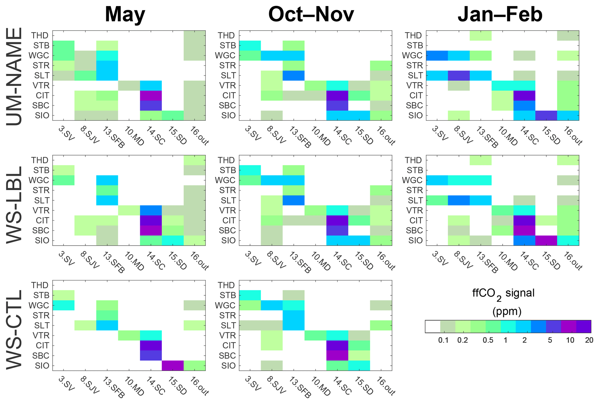
Figure 2The average ffCO2 signal (ppm) simulated by each atmospheric transport model as a result of emissions from the six largest emitting air basins and one region outside California (denoted as 16.out) at each observation site over the three measurement campaigns. Signals were simulated based on the EDGAR emission map.
3.1 Simulated ffCO2 observations
Before presenting the results of the inversion experiments, we first examine simulated ffCO2 contributions in different regions at each of the nine observation sites. This allows us to quantify which air basins have the largest influence on simulated concentrations at observation sites and better interpret the results of the experiments. Figure 2 shows simulated concentrations at observation sites resulting from emissions in the six highest-emitting air basins in California and from outside California. The highest signals (>10 ppm) are simulated at urban sites (e.g. CIT – Caltech – and SBC – San Bernardino) for emissions from urban air basins (e.g. South Coast, 14.SC). The nine air basins not shown in Fig. 2 contributed signals below 0.1 ppm due to the small size or low emissions of the air basin (e.g. Lake County and Lake Tahoe) or distance from the observation network (e.g. Northeast Plateau, Great Basin valleys, and Salton Sea). In general, the northern sites (THD to SLT in Fig. 2) are sensitive to northern air basins (Sacramento and San Joaquin valleys and SF Bay), and the southern sites (VTR to Scripps Institute of Oceanography – SIO) are sensitive to emissions from southern air basins (Mojave Desert, South Coast, and San Diego). All transport models show that the observation sites are sensitive to more air basins in the October–November and January–February campaigns compared to the May campaign (Fig. 2). Signals simulated by WS-CTL come from fewer air basins than UM-NAME or WS-LBL, particularly in May.
In our simulation experiments, signals from outside California are generally small compared to the total signal for most sites (<10 % on average), although they can average from 20 %–50 % for Sutter Buttes (STB), STR, SLT and SIO for individual campaigns. For THD, located near the northern border of the state, a larger influence from outside California is found to be 10 %–90 %, due to a combination of relatively low local emissions and northerly winds transporting emissions from the northwestern United States and Canada.
3.1.1 Difference in magnitude of emissions
Figure 3a shows the statewide inversion result for the experiment testing the effect of a bias in magnitude in regional emissions in the prior simulation. In this figure, and in similar figures that follow for the other experiments, prior estimates are represented by black markers and posterior estimates are represented by coloured markers, with the 2σ uncertainty on the x axis and the bias relative to the truth on the y axis. The diagonal lines show 1:1 and lines so that a marker lying to the right of these lines indicates the posterior bias is smaller than the posterior uncertainty, whereas a marker to the left of these lines indicates the posterior bias is larger than the posterior uncertainty. Filled markers show results using SD prior uncertainty, and empty markers show results using 70 % prior uncertainty. Prior and posterior uncertainties are expressed as 2σ.
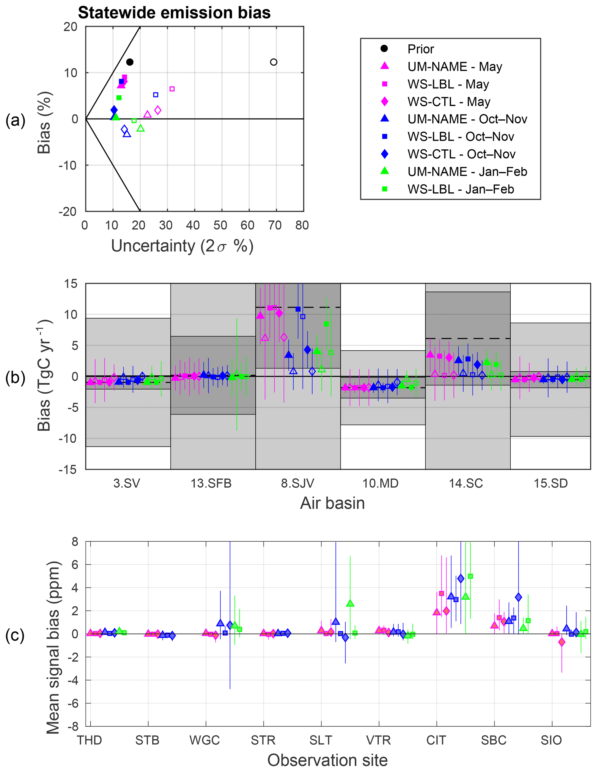
Figure 3(a) Statewide and (b) individual air basin inversion results for an error in the magnitude of prior emissions. Prior emissions are given by EDGAR, and true emissions are given by EDGAR scaled to Vulcan total in each air basin. Air basin results are shown for Sacramento Valley (3.SV), San Francisco Bay (13.SFB), San Joaquin Valley (8.SJV), Mojave Desert (10.MD), South Coast (14.SC), and San Diego (15.SD). Prior results are presented by black markers, and posterior results are represented by coloured markers. Filled markers show results using SD prior uncertainty, and empty markers show results using 70 % prior uncertainty. The prior bias in each air basin is given by the dashed lines in (b), with SD prior uncertainty (dark grey) and 70 % prior uncertainty (light grey). Prior and posterior uncertainties are expressed as 2σ. The bottom plot (c) shows the mean signal error in simulated average ffCO2 concentration. Mean signal error is calculated by subtracting the average true signal from the average prior signal. Error lines are drawn between the maximum and minimum signal bias per campaign.
For all transport models and campaigns, the inversion is able to reduce prior bias and scale posterior emissions towards the truth. The +12 % bias in the statewide emissions in the prior was reduced to a posterior bias of between 0 % and +9 % (mean bias is +5 %) for SD prior uncertainty. Using 70 % prior uncertainty reduced prior bias to between −3 and +6 (mean is +1 %). Statewide posterior uncertainty was 10 %–14 % (mean 12 %) and 14 %–32 % (mean is 21 %) for the SD and 70 % prior uncertainty respectively, where uncertainty is expressed as 2σ, lower than the statewide prior uncertainties of 16 % for the SD and 69 % for 70 % prior uncertainty. There were no outliers identified in this experiment.
To determine what is driving the statewide results, we examine the individual air basin inversion results. Figure 3b shows the inversion results for the six main emission regions of California, with the San Joaquin Valley (8.SJV) and South Coast (14.SC) having the largest prior biases. For the San Joaquin Valley (8.SJV) and South Coast (14.SC) regions with the largest prior bias, the biases are reduced in most cases; however, only the posterior estimates from the 70 % prior uncertainty experiment overlap the true emissions. The posterior estimates for SD prior uncertainty do not overlap with the truth, indicating that the 2σ prior uncertainty of 24 % in South Coast (14.SC), for example, restricts the inversion from eliminating biases of 30 % in these regions (Table 1), given the observations available. The nine air basins omitted from Fig. 3b are generally not being scaled by the inversion due to a lack of constraint from the observation network, low emissions, or small prior uncertainty (Fig. S1 in the Supplement).
The bias in the posterior estimate of statewide emissions is larger in May than in October–November and January–February (Fig. 3a, triangles). This poorer performance of the inversion in May can be largely attributed to the San Joaquin Valley (8.SJV), where the posterior emissions are largely unchanged from the prior in May. There is no observation site in the San Joaquin Valley, and as shown in Fig. 2, emissions in the San Joaquin Valley do not reach observation sites in neighbouring air basins in May, but they do reach these sites in October–November and January–February. In contrast, the South Coast (14.SC) influences the two observation sites, CIT and SBC, located in the region as well as several other sites (Fig. 2). Both CIT and SBC show that prior signals are too high compared to true signals for all campaigns and models (Fig. 3c), reflecting the positive bias in prior emissions in the South Coast region, which is reduced in the posterior. Changing the uncertainty parameter from 0.5 to 0.3 or 0.8 had the result of decreasing the ability of the inversion to scale statewide emissions towards true emissions by 1 %–4 %, with an increase in posterior uncertainty by a similar percentage.
3.1.2 Difference in spatial distribution of emissions
The statewide inversion results for the experiment, including errors in the spatial distribution of emissions, are shown in Fig. 4a. In this case the magnitude of prior emissions in each air basin is equal to true emissions, and we aim to quantify how errors in the spatial distribution of emissions (EDGAR as prior and Vulcan as true distribution) lead to bias in posterior emission estimates. Posterior emissions are negatively biased, apart from WS-LBL in January–February. Posterior bias was between −10 % and +1 % (mean is −4 %) for SD prior uncertainty and between −10 % and +4 % (mean is −4 %) for 70 % prior uncertainty across transport models and campaigns. As might be expected from the experimental set-up with an unbiased prior, posterior emission estimates generated using SD prior uncertainty have a smaller mean bias and smaller range of posterior estimates compared to those generated using 70 % prior uncertainty. Statewide uncertainty was reduced from 16 % to 10 %–14 % (mean is 12 %) for SD prior uncertainty and from 58 % to 14 %–21 % (mean is 18 %) for 70 % air basin prior uncertainty. Biases induced are smaller than the 2σ posterior uncertainty across all transport models, campaigns, and choices of prior uncertainty.
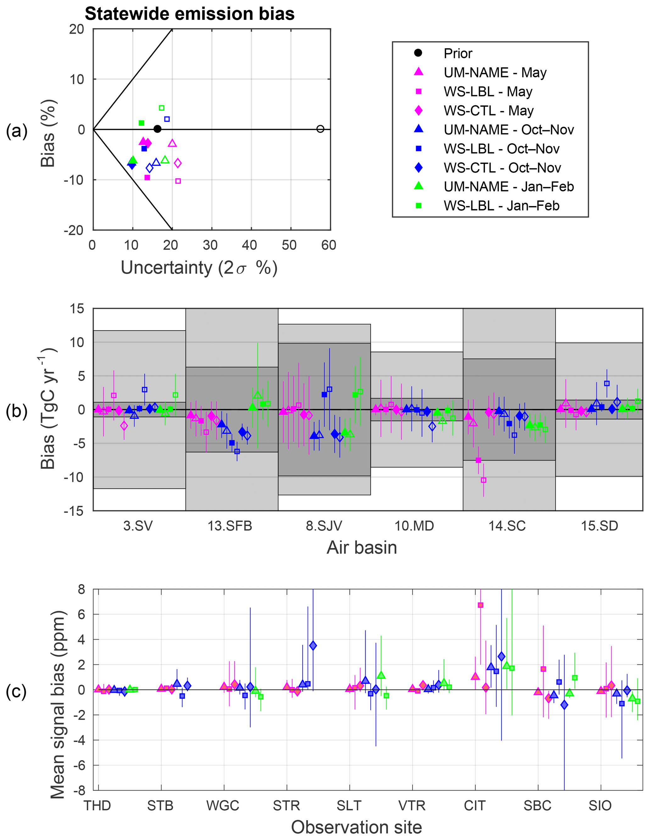
Figure 4(a) Statewide and (b) individual air basin inversion results for an error in the spatial distribution of prior emissions. Prior emissions are given by EDGAR scaled to Vulcan emission totals in each air basin, and true emissions are given by Vulcan; (c) shows the mean signal error in simulated average ffCO2 concentration.
Posterior emission results in the two largest emitting air basins (the San Francisco Bay and South Coast) are also negatively biased in most cases (Fig. 4b). In several cases, posterior biases are larger than the associated posterior uncertainties, for example in the South Coast for WS-LBL in all cases. Considering Fig. 4c, prior ffCO2 signals are being overestimated more often than underestimated, particularly for the relatively more urban sites CIT and SLT.
Since the prior emissions from EDGAR have been scaled to have the same total as Vulcan (the true emissions) in each region, the pattern of more negative posterior emissions is only caused by the subregional spatial distribution of emissions. Comparing Vulcan and EDGAR native grid cell emissions in Figs. 1c and S2, EDGAR tends to have greater emissions in high-emission grid cells. In other words, the emissions are more concentrated in EDGAR and more dispersed in Vulcan. This pattern explains the negative bias in posterior emissions for the urban South Coast air basin. The opposite effect does not appear to hold for rural observation sites and regions, perhaps because rural emissions are already rather dispersed and have less of an influence on the observations.
In these experiments, 0 %–3 % of observations were identified as outliers, but excluding outliers did not change the statewide result significantly (<1 % change in mean bias).
3.1.3 Difference in temporal variation of emissions
Figure 5a shows the statewide inversion result for the experiment where the emissions are Vulcan temporally varying in the prior simulation (see Fig. 1b) but are Vulcan temporally invariant in the true simulation. Posterior bias was between −13 % and +5 % (mean is −3 %) for SD uncertainty and between −15 % and +6 % (mean is −3 %) for 70 % prior uncertainty. Posterior uncertainty was 11 %–15 % (mean is 12 %) for SD prior uncertainty and was 15 %–24 % (mean is 18 %) in posterior emissions for SD (70 %) prior uncertainty. Outlier removal resulted in 0 %–1 % (mean is 0 %) of data points being removed, which did not change the statewide results.
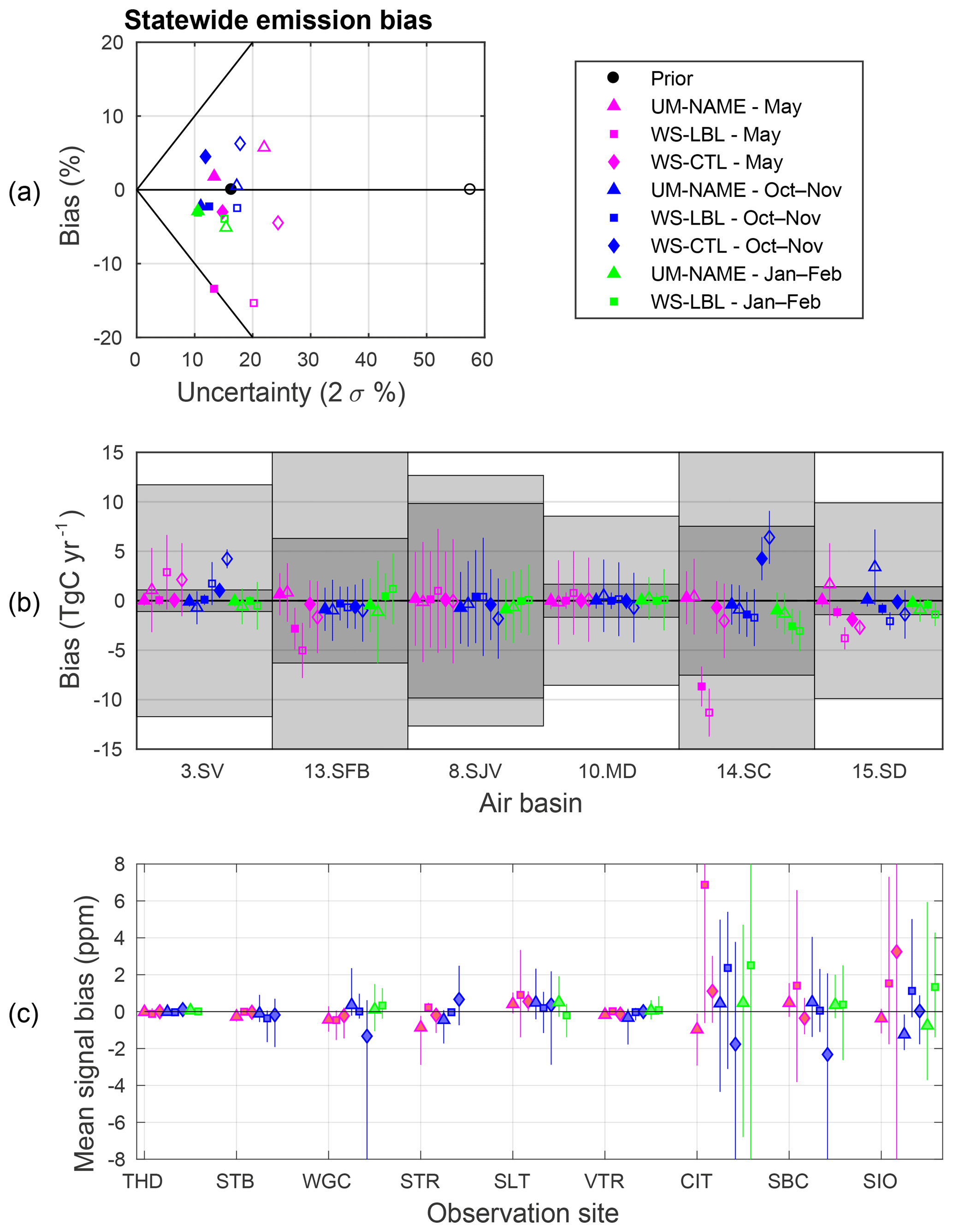
Figure 5(a) Statewide and (b) individual air basin inversion results for an error in the temporal distribution of prior emissions. Prior emissions are given by temporally varying Vulcan and true emissions are given by annually averaged Vulcan. Prior emissions were scaled to be equal in magnitude to annually averaged Vulcan emissions; (c) shows the mean signal error in simulated average ffCO2 concentration.
The posterior estimate for WS-LBL in May with SD prior uncertainty has a significant negative bias of −13 %, approximately the same magnitude as the associated 2σ posterior uncertainty. As can be seen by the air basin results of Fig. 5b, the statewide bias for WS-LBL in May is being driven by a large regional bias in the South Coast but also in the San Francisco Bay and San Diego air basins. These regional biases are larger than their associated posterior uncertainties. Figure 5c shows that the prior ffCO2 signals at CIT average ∼7 ppm too high in May for WS-LBL. In contrast, prior ffCO2 signals at CIT and SBC are too low in October–November for WS-CTL, leading to a high bias in posterior emissions from the South Coast. San Diego also exhibited both high and low biases in the posterior emissions. Overall, temporal variations in emissions led to posterior biases generally within ±6 % but as large as 15 %; however, a consistent pattern in the posterior bias due to the temporal representation in emissions was not found.
3.1.4 Difference in atmospheric transport
The statewide inversion results for the experiment where the atmospheric transport in the prior simulation uses WS-CTL or UM-NAME but the atmospheric transport in the true simulation uses WS-LBL are shown in Fig. 6a. Outliers were identified in these experiments, and we present results for inversions including all data and for inversions where outliers were removed.
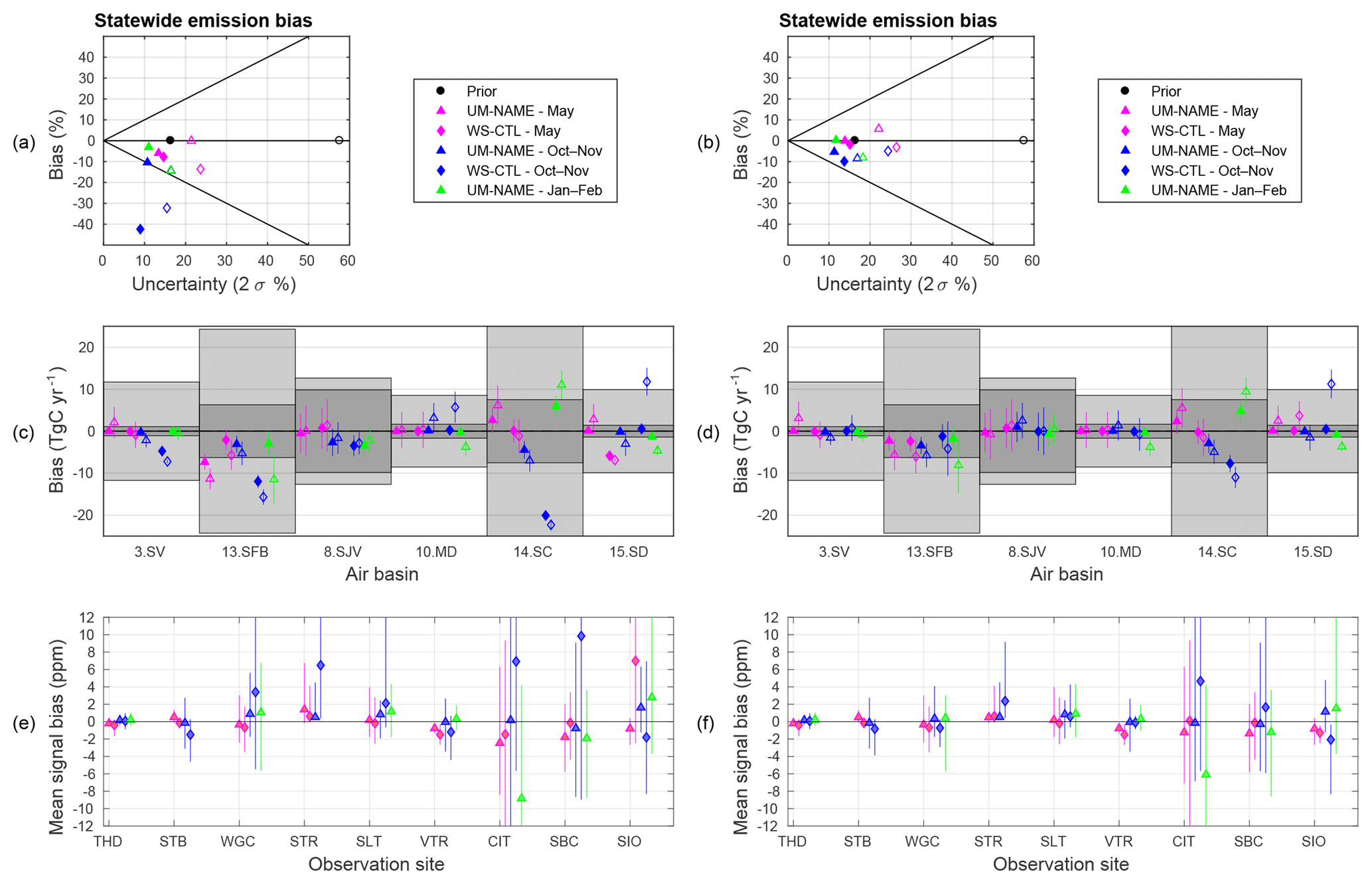
Figure 6Inversion results for the experiment where the atmospheric transport in the prior simulation uses WS-CTL or UM-NAME, but the atmospheric transport in the true simulation uses WS-LBL. Posterior statewide emissions (a, b), individual air basin emissions (c, d), and percentage error in simulated average ffCO2 concentration (e, f) are shown with no outlier removal (a, c, e) and outliers removed (b, d, f). Prior and true emissions are given by annually averaged Vulcan emissions.
When all data are included, differences in the atmospheric transport model introduce a bias in statewide posterior emissions of between −42 % and −3 % (mean is −12 %) for SD prior uncertainty and between −32 % and 0 % (mean is −15 %) for 70 % prior uncertainty. For one case, using WS-CTL to generate prior signals in October–November, the bias in the posterior emission estimate was larger than the 2σ uncertainty for both the SD and 70 % prior uncertainty. Changing the uncertainty parameter from 0.5 to 0.3 or 0.8 resulted in posterior emissions remaining closer to true emissions by 0 %–4 % and increasing the posterior uncertainty by 1 %–5 %.
Removing outliers significantly improved the inversion results (Fig. 6b); the mean bias was between −10 % and 0 % (mean is −3 %) for SD prior uncertainty and between −9 % and +6 % (mean is −5 %) for 70 % prior uncertainty when outliers were removed. Posterior uncertainty was 9 %–15 % (mean is 12 %) and 15 %–24 % (mean is 18 %) for the SD and 70 % prior uncertainty respectively, with all posterior estimates within 2σ of the true statewide emissions. The reduction in posterior bias when outliers are removed is mostly due to the removal of a few large positive outliers in prior simulated signals by WS-CTL (Fig. 7). Figure 7 illustrates the time series of simulated ffCO2 in each model, with outliers shown as an x. Outliers removed were between 6.9 % and 20.6 % of all observations (mean is 10.5 %). This is similar to the fraction of outliers identified in Graven et al. (2018) using the same method with real data (∼8 %). It is also similar to that of Jeong et al. (2012a, b; 0 %–27 %) for monthly inversions of CH4 in California using a different method of identifying outliers where model-data residuals are larger than 3σ of model-data uncertainty. This is an important result for the atmospheric inversion community working at such spatial scales, as it highlights the benefits of removing outliers.
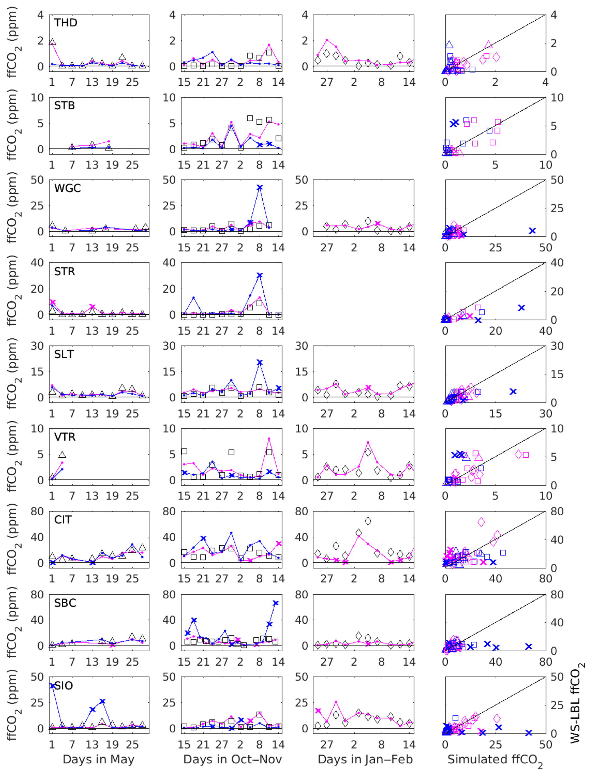
Figure 7All simulated ffCO2 from May (first column), October–November (second column), and January–February (third column). Simulated ffCO2 values using WS-LBL are shown in black markers (triangles for May, squares for October–November, and diamonds for January–February), whilst prior WS-CTL signals are shown in blue and UM-NAME signals are shown in magenta. All simulated signals are generated using the Vulcan gridded emission map. The fourth column shows true vs. prior ffCO2 signals, with colours corresponding to models and markers corresponding to campaigns. Outliers omitted from the standard inversion are shown with an x.
While the statewide posterior emission estimate is significantly biased in only one case (WS-CTL in October–November) when outliers are not removed, the posterior emission estimates for the main emission regions are significantly biased in several cases (Fig. 6c). The largest bias is in the South Coast region, where posterior estimates are biased by more than −75 % (with 1 % posterior uncertainty) in October–November when using WS-CTL to generate prior signals. This large posterior emission bias in the South Coast and the statewide total can be attributed to overestimates in the prior ffCO2 signal of more than 6 ppm on average at CIT and SBC and more than 2 ppm at WGC and STR (Fig. 6e) due to some high outliers in the WS-CTL simulations (Fig. 7). Posterior estimates for San Francisco Bay, South Coast, and San Diego were also significantly biased in some other cases, particularly for 70 % prior uncertainty but also for SD prior uncertainty. This indicates that regional biases caused by differences in atmospheric transport appear to compensate over the statewide scale and that results for individual regions are less robust than aggregate results for the statewide network. It also suggests that an observation network with multiple sites in a variety of settings is beneficial for reducing the impact of uncertainty in atmospheric transport.
To investigate the differences in simulated ffCO2 and to assess whether these could be attributed to specific aspects of modelled meteorology, we compared the PBLH and wind speed in WS-LBL and the UM for five of the nine observation sites where the PBLH output was available. PBLH was not available for WS-CTL. Estimates for the PBLH in WS-LBL are based on the MYNN2 parameterization scheme that estimates the PBLH using localized turbulence kinetic-energy closure parameterization (Nakanishi and Niino, 2004, 2006). Estimates of the PBLH are calculated internally within the UM. The PBLH and wind speed were averaged over 6 h from 12:00 to 18:00 PST to compare the afternoon means (Seibert et al., 2000). We found no consistent correlation between differences in the PBLH or wind speed and differences in simulated ffCO2 between models across sites and campaigns (Fig. S3). Absolute values of wind direction and ffCO2 did not show consistent correlations either. The lack of correlation suggests that we cannot attribute differences in simulated ffCO2 to any single meteorological variable estimated at any individual station in the transport models.
We also examined if differences in simulated ffCO2 signals across transport models could be explained by the differences in spatial resolution of the models. WS-CTL footprints were re-gridded from a 0.1∘ native grid to the coarser UM-NAME grid of 17 or 25 km and were then used to simulate ffCO2. For this comparison, we simulated ffCO2 every day over the campaign period. We found no consistent reduction in mean ffCO2 bias between sites over the two campaigns, however there is a reduction in spread of bias at four sites for both campaigns (WGC, SLT, SBC, and SIO), suggesting that the model resolution could potentially have an impact for these sites. In general however, we cannot say that transport model resolution error in atmospheric transport is a key driver of ffCO2 signal bias across observation sites (Fig. S4).
Our results show that atmospheric inversions can reduce a hypothetical bias in the magnitude of prior ffCO2 emission estimates for the US state of California using the ground-based observation network from Graven et al. (2018), under the idealized assumptions of perfect atmospheric transport and perfect spatio-temporal distribution of emission in the prior estimate. By exploring differences in model transport and spatio-temporal distribution of prior emissions, we found that biases of magnitudes of 1 %–15 % in monthly posterior estimates of statewide emissions can result from differences in the temporal variation, spatial distribution, and modelled transport of the prior simulation. However, these biases were less than the 2σ posterior uncertainty in total state emissions when outliers were removed. In some cases, the biases in posterior emissions for individual air basins were significant compared to the posterior uncertainties, suggesting that estimates for individual regions are less reliable than the aggregate estimates of the statewide total.
The largest bias in statewide posterior estimates was found to be caused by errors in the temporal variation in emissions. This highlights the necessity for temporally varying emissions to be estimated and included in prior emission estimates, particularly for urban regions. Similar results have been found in other regions including Indianapolis (Turnbull et al., 2015) and Europe (Peylin et al., 2011) and, more generally, for high-emission regions around the globe (Zhang et al., 2016). Although the afternoon sampling is near to the diurnal maximum in emissions in California (Fig. 1c, Gurney et al., 2009), which might be expected to lead to higher simulated ffCO2 in temporally varying vs. temporally invariant emissions, we did not find consistently positive biases in ffCO2 but rather both positive and negative biases. This suggests that the overall impact of temporally varying emissions depends on the model transport and the characteristics of the observation site. Furthermore, uncertainties in the temporal distribution of emissions at an hourly resolution have not yet been fully quantified (Nassar et al., 2013).
Errors in model transport, as represented in our experiments by using different transport models, were shown to bias posterior ffCO2 emissions by 10 % or less when outliers were removed. These biases related to transport error are somewhat lower than estimated by similar simulation experiments for ffCO2 emission estimates for the US by Basu et al. (2016) using different transport models (>10 %), although their spatial scale was larger and the alternate model they used was intentionally biased. In contrast, the three models we use are all actively applied in regional greenhouse gas inversions. Our results are comparable to the estimate of ±15 % uncertainty in atmospheric transport in WS-LBL using comparisons with atmospheric observations of carbon monoxide (CO) in California (Bagley et al., 2017).
The fraction of pseudo-observations we identified as outliers in these transport error experiments (10.5 %, range of 6.9 %–20.6 %) was similar to Graven et al. (2018), where 8 % of all observations were removed as outliers using the same method. The outliers in our experiments were primarily high ffCO2 signals simulated by WS-CTL in October–November. When included in the inversion, these did lead to significant biases in the posterior estimates for the experiment on model transport. This highlights the need for careful examination of simulated ffCO2 and consideration of outliers in atmospheric ffCO2 inversions.
Attributing differences in simulated ffCO2 between the different transport models to specific meteorological variables proved inconclusive, and model resolution error did not appear to explain the differences in simulated signals, although we were not able to investigate aggregation error in comparison to the high-resolution WS-LBL model. Wang et al. (2017) found aggregation error to be only a minor contributor to errors in simulated ffCO2 in Europe, while Feng et al. (2016) found that high-resolution gridded emission estimates could be more important than high-resolution transport models for simulations of greenhouse gases in the greater Los Angeles area. We found that differences in the spatial representation of prior emissions in EDGAR compared to Vulcan led to consistently lower, although not significantly different, posterior statewide estimates due to the emissions in EDGAR being more concentrated in urban regions. The spatial allocation of emissions between urban and rural regions in gridded emission estimates have much larger percentage uncertainties than national totals (Hogue et al., 2016), suggesting that several different gridded emission estimates should be used in regional ffCO2 inversions to capture this source of uncertainty.
The results of these experiments suggest that the choice of a prior emission estimate and transport model (among those considered here and currently used in the community) used in our ffCO2 inversion would result in differences of 15 % or less in posterior statewide ffCO2 emissions in California, using the observation network from Graven et al. (2018). These differences are generally not significant, compared to the posterior 2σ uncertainties of 10 % to 15 %. In comparison, Graven et al. (2018) found that posterior statewide ffCO2 emissions were not statistically different when using temporally varying emissions from Vulcan, as compared to annual mean emissions from Vulcan or EDGAR, with posterior uncertainties of ±15 % to ±17 %. Our results may be specific to the California region, observation network, and inversion set-up we consider here, but we expect that similar differences of 1 %–15 % are likely to be found elsewhere in similar inversions at comparable regional scales. We note that while we have assessed individual contributions to uncertainty in the experiments formulated here, these contributions can also interact with each other. These interactions could act to increase the resulting biases, or partly cancel them, depending on the combination used. The possibility of interacting effects implies that multiple prior emission estimates and transport models should be used in inversions of real data.
In our results, emissions from many small or rural air basins did not have a significant contribution to the local enhancement of ffCO2 at the observation sites and were not adjusted by the inversion in most cases (Figs. 2 and S1). Combined with our experimental set-up specifying the magnitude of prior emissions to be equal to true emissions, it might be expected that our results could underestimate the predicted biases in posterior emissions. However, these experiments were designed specifically for quantifying representation and transport error using the inversion set-up and the observation network from Graven et al. (2018) as a test case. Here, we have assumed the model–measurement mismatch uncertainty matrix is diagonal, following previous work (e.g. Gerbig et al., 2003; Fischer et al., 2017), however the consideration of correlated errors in the uncertainty matrix has also been found to affect posterior emissions for methane in California and reduce their uncertainty at the level of several percent (Jeong et al., 2016). Fischer et al. (2017) showed in individual simulation experiments that using either EDGAR or a spatially uniform flux of 1 µmol m−2 s−1 as a biased prior produced posterior emissions that were substantially closer to true emissions, but only if the prior uncertainties are set large enough to encompass biases in prior emissions. Therefore, further experiments using a different experimental set-up such as choice of mismatch error or specification of inversion regions (e.g. to change the inversion region size based on proximity to the observation network; Manning et al., 2011) would help to characterize uncertainties in regional ffCO2 inversions and the robustness of posterior estimates to the choices made in the inversion set-up.
We have shown that atmospheric inversions for the US state of California can reduce a hypothetical bias in the magnitude of prior emission estimates of ffCO2 in California using the ground-based observation network from Graven et al. (2018). Experiments for characterizing the effect of differences in the spatial and temporal distribution in prior emissions resulted in biases in posterior total state emissions with magnitudes of 1 %–15 %, similar to monthly posterior estimates of Basu et al. (2016) for the western US. Our results highlight the need for (1) temporal variation to be included in prior emissions, (2) different estimates of the spatial distribution of emissions between urban and rural regions to be considered, and (3) representation of atmospheric transport in regional ffCO2 inversions to be further evaluated.
Data and code related to the Bayesian inversion procedure can be made available upon request.
The supplement related to this article is available online at: https://doi.org/10.5194/acp-19-2991-2019-supplement.
Prior and simulated concentrations of fossil fuel CO2, along with all code to run the inversion and all graphics, were produced in MATLAB by KB. KB ran the UM-NAME transport model under guidance from AJM and TA. MLF, SJ, and XC produced concentrations from the WS-LBL transport model coupled with EDGAR and Vulcan. Guidance on the coupling of temporally varying emissions and the UM-NAME transport model was provided by EW and MR. HG was the main scientific supervisor, oversaw all implementation of the inversion, and provided guidance on the presentation of results. KB was responsible for the development of the paper, which forms part of his PhD. All authors had the opportunity to comment on the paper.
The authors declare that they have no conflict of interest.
This article is part of the special issue “The 10th International Carbon Dioxide Conference (ICDC10) and the 19th WMO/IAEA Meeting on Carbon Dioxide, other Greenhouse Gases and Related Measurement Techniques (GGMT-2017; AMT/ACP/BG/CP/ESD inter-journal SI)”. It is a result of the 10th International Carbon Dioxide Conference, Interlaken, Switzerland, 21–25 August 2017.
This project was funded by the Grantham Institute – Climate Change and the
Environment Science and Solutions for a Changing Planet DTP (NE/L002515/1),
the Natural Environment Research Council (NERC, UK), the UK Met Office, the NASA
Carbon Monitoring System (NNX13AP33G and NNH13AW56I), and the European Commission
through a Marie Curie Career Integration Grant. The authors thank Arlyn E. Andrews
and the CarbonTracker-Lagrange team for providing footprints. Support for
CarbonTracker-Lagrange has been provided by the NOAA Climate Program
Office's Atmospheric Chemistry, Carbon Cycle, and Climate (AC4) program and
the NASA Carbon Monitoring System.
Edited by: Nicolas Gruber
Reviewed by: Sourish Basu and one anonymous referee
Andres, R. J., Boden, T. A., Bréon, F.-M., Ciais, P., Davis, S., Erickson, D., Gregg, J. S., Jacobson, A., Marland, G., Miller, J., Oda, T., Olivier, J. G. J., Raupach, M. R., Rayner, P., and Treanton, K.: A synthesis of carbon dioxide emissions from fossil-fuel combustion, Biogeosciences, 9, 1845–1871, https://doi.org/10.5194/bg-9-1845-2012, 2012.
Asefi-Najafabady, S., Rayner, P. J., Gurney, K. R., McRobert, A., Song, Y., Coltin, K., Huang, J., Elvidge, C., and Baugh, K.: A multiyear, global gridded fossil fuel CO2 emission data product: Evaluation and analysis of results, J. Geophys. Res.-Atmos., 119, 10213–10231, https://doi.org/10.1002/2013JD021296, 2014.
Bagley, J. E., Jeong, S., Cui, X., Newman, S., Zhang, J., Priest, C., Campos-Pineda, M., Andrews, A. E., Bianco, L., Lloyd, M., and Lareau, N.: Assessment of an atmospheric transport model for annual inverse estimates of California greenhouse gas emissions, J. Geophys. Res.-Atmos., 122, 1901–1918, https://doi.org/10.1002/2016JD025361, 2017.
Basu, S., Miller, J. B., and Lehman, S.: Separation of biospheric and fossil fuel fluxes of CO2 by atmospheric inversion of CO2 and 14CO2 measurements: Observation System Simulations, Atmos. Chem. Phys., 16, 5665–5683, https://doi.org/10.5194/acp-16-5665-2016, 2016.
Boden, T., Andres, B., and Marland, G.: Global CO2 Emissions from Fossil-Fuel Burning, Cement Manufacture, and Gas Flaring: 1751–2014, Carbon Dioxide Information Analysis Center, available at: https://cdiac.ess-dive.lbl.gov/ftp/ndp030/global.1751_2014.ems (last access: 1 March 2019), 2017.
CARB: California Greenhouse Gas Emission Inventory – 2017 Edition, California Air Resources Board, available at: http://www.arb.ca.gov/cc/inventory/data/data.htm (last access: 1 March 2019), 2018.
Chen, F. and Dudhia, J.: Coupling an Advanced Land Surface Hydrology Model with the Penn State NCAR MM5 Modeling System. Part 1: Model Implementation and Sensitivity, Mon. Weather Rev., 129, 569–585, 2001.
Chevallier, F., Maksyutov, S., Bousquet, P., Bréon, F.-M., Saito, R., Yoshida, Y., and Yokota, T.: On the accuracy of the CO2 surface fluxes to be estimated from the GOSAT observations, Geophys. Res. Lett., 36, L19807, https://doi.org/10.1029/2009GL040108, 2009.
Cullen, M. J. P.: The Unified Forecast/Climate Model, Meteorol. Mag., 1449, 81–94, 1993.
EDGAR: EDGAR Greenhouse Gas Emissions Inventory v4.2 FT2010, available at: http://edgar.jrc.ec.europa.eu/index.php (last access: 1 March 2019), 2011.
Feng, S., Lauvaux, T., Newman, S., Rao, P., Ahmadov, R., Deng, A., Díaz-Isaac, L. I., Duren, R. M., Fischer, M. L., Gerbig, C., Gurney, K. R., Huang, J., Jeong, S., Li, Z., Miller, C. E., O'Keeffe, D., Patarasuk, R., Sander, S. P., Song, Y., Wong, K. W., and Yung, Y. L.: Los Angeles megacity: a high-resolution land–atmosphere modelling system for urban CO2 emissions, Atmos. Chem. Phys., 16, 9019–9045, https://doi.org/10.5194/acp-16-9019-2016, 2016.
Fischer, M. L., Parazoo, N., Brophy, K., Cui, X., Jeong, S., Liu, J., Keeling, R., Taylor, T. E., Gurney, K., Oda, T., and Graven, H.: Simulating estimation of California fossil fuel and biosphere carbon dioxide exchanges combining in situ tower and satellite column observations, J. Geophys. Res.-Atmos., 122, 3653–3671, https://doi.org/10.1002/2016JD025617, 2017.
Gerbig, C., Lin, J. C., Wofsy, S. C., Daube, B. C., Andrews, A. E., Stephens, B. B., Bakwin, P. S., and Grainger, C. A.: Toward constraining regional-scale fluxes of CO2 with atmospheric observations over a continent: 2. Analysis of COBRA data using a receptor-oriented framework, J. Geophys. Res.-Atmos., 108, 4757, https://doi.org/10.1029/2003JD003770, 2003.
Graven, H. D., Fischer, M. L., Lueker, T., Jeong, S., Guilderson, T. P., Keeling, R. F., Bambha, R., Brophy, K., Callahan, W., Cui, X., and Frankenberg, C.: Assessing fossil fuel CO2 emissions in California using atmospheric observations and models, Environ. Res. Lett., 13, 065007, https://doi.org/10.1088/1748-9326/aabd43, 2018.
Grell, G. A., Dudhia, J., and Stauffer, D. R.: A description of the fifth-generation Penn State/NCAR Mesoscale Model (MM5), NCAR Technical Note NCAR/TN-398+STR, https://doi.org/10.5065/D60Z716B, 1994.
Gurney, K. R., Law, R. M., Denning, A. S., Rayner, P. J., Baker, D., Bousquet, P., Bruhwiler, L., Chen, Y. H., Ciais, P., Fan, S., and Fung, I. Y.: TransCom 3 CO2 inversion intercomparison: 1. Annual mean control results and sensitivity to transport and prior flux information, Tellus B, 55, 555–579, https://doi.org/10.1034/j.1600-0889.2003.00049.x, 2003.
Gurney, K. R., Mendoza, D. L., Zhou, Y., Fischer, M. L., Miller, C. C., Geethakumar, S., and de la Rue du Can, S.: High resolution fossil fuel combustion CO2 emission fluxes for the United States, Environ. Sci. Technol., 43, 5535–5541, https://doi.org/10.1021/es900806c, 2009.
Hogue, S., Marland, E., Andres, R. J., Marland, G., and Woodard, D.: Uncertainty in gridded CO2 emissions estimates, Earth's Future, 4, 225–239, https://doi.org/10.1002/2015EF000343, 2016.
Hong, S. Y., Noh, Y., and Dudhia, J.: A new vertical diffusion package with an explicit treatment of entrainment processes, Mon. Weather Rev., 134, 2318–2341, https://doi.org/10.1175/MWR3199.1, 2006.
Hungershoefer, K., Breon, F.-M., Peylin, P., Chevallier, F., Rayner, P., Klonecki, A., Houweling, S., and Marshall, J.: Evaluation of various observing systems for the global monitoring of CO2 surface fluxes, Atmos. Chem. Phys., 10, 10503–10520, https://doi.org/10.5194/acp-10-10503-2010, 2010.
Jeong, S., Zhao, C., Andrews, A. E., Bianco, L., Wilczak, J. M., and Fischer, M. L.: Seasonal variation of CH4 emissions from central California, J. Geophys. Res., 117, D11306, https://doi.org/10.1029/2011JD016896, 2012a.
Jeong, S., Zhao, C., Andrews, A. E., Dlugokencky, E. J., Sweeney, C., Bianco, L., Wilczak, J. M., and Fischer, M. L.: Seasonal variations in N2O emissions from central California, Geophys. Res. Lett., 39, L16805, https://doi.org/10.1029/2012GL052307, 2012b.
Jeong, S., Hsu, Y. K., Andrews, A. E., Bianco, L., Vaca, P., Wilczak, J. M., and Fischer, M. L.: A multitower measurement network estimate of California's methane emissions, J. Geophys. Res.-Atmos., 118, 11339–11351, https://doi.org/10.1002/jgrd.50854, 2013.
Jeong, S., Newman, S., Zhang, J., Andrews, A. E., Bianco, L., Bagley, J., Cui, X., Graven, H., Kim, J., Salameh, P., LaFranchi, B. W., Priest, C., Campos-Pineda, M., Novakovskaia, E., Sloop, C. D., Michelsen, H. A., Bambha, R. P., Weiss, R. F., Keeling, R., and Fischer, M. L.: Estimating methane emissions in California's urban and rural regions using multitower observations, J. Geophys. Res.-Atmos., 121, 13031–13049, https://doi.org/10.1002/2016JD025404, 2016.
Jones, A., Thomson, D., Hort, M., and Devenish, B.: The U.K. Met Office's Next-Generation Atmospheric Dispersion Model, NAME III, in: Air Pollution Modeling and Its Application XVII, edited by: Borrego C. and Norman, A. L., Springer, Boston, MA, https://doi.org/10.1007/978-0-387-68854-1_62, 2007.
Lauvaux, T., Miles, N. L., Deng, A., Richardson, S. J., Cambaliza, M. O., Davis, K. J., Gaudet, B., Gurney, K. R., Huang, J., O'Keefe, D., Song, Y., Karion, A., Oda, T., Patarasuk, R., Razlivanov, I., Sarmiento, D., Shepson, P., Sweeney, C., Turnbull, J., and Wu, K.: High-resolution atmospheric inversion of urban CO2 emissions during the dormant season of the Indianapolis Flux Experiment (INFLUX), J. Geophys. Res.-Atmos., 121, 5213–5236, https://doi.org/10.1002/2015JD024473, 2010.
Levin, I., Kromer, B., Schmidt, M., and Sartorius, H.: A novel approach for independent budgeting of fossil fuel CO2 over Europe by 14CO2 observations, Geophys. Res. Lett., 30, 2194, https://doi.org/10.1029/2003GL018477, 2003.
Lin, J. C., Gerbig, C., Wofsy, S. C., Andrews, A. E., Daube, B. C., Davis, K. J., and Grainger, C. A.: A near-field tool for simulating the upstream influence of atmospheric observations: The Stochastic Time-Inverted Lagrangian Transport (STILT) model, J. Geophys. Res.-Atmos., 108, 4493, https://doi.org/10.1029/2002JD003161, 2003.
Liu, J., Bowman, K., Lee, M., Henze, D., Bousserez, N., Brix, H., Collatz, G. J., Menemenlis, D., Ott, L., Pawson, S., Jones, D., and Nassar, R.: Carbon monitoring system flux estimation and attribution: impact of ACOS-GOSAT XCO2 sampling on the inference of terrestrial biospheric sources and sinks, Tellus B, 66, 22486, https://doi.org/10.3402/tellusb.v66.22486, 2014.
Guan, D., Liu Z., Geng, Y., Lindner, S., and Hubacek, K.: The gigatonne gap in China's carbon dioxide inventories, Nat. Clim. Change, 2, 672–675, https://doi.org/10.1038/nclimate1560, 2012.
Manning, A. J., O'Doherty, S., Jones, A. R., Simmonds, P. G., and Derwent, R. G.: Estimating UK methane and nitrous oxide emissions from 1990 to 2007 using an inversion modeling approach, J. Geophys. Res.-Atmos., 116, D02305, https://doi.org/10.1029/2010JD014763, 2011.
Marland, G., Brenkert, A., and Olivier, J.: CO2 from fossil fuel burning: a comparison of ORNL and EDGAR estimates of national emissions, Environ. Sci. Policy, 2, 265–273, https://doi.org/10.1016/S1462-9011(99)00018-0, 1999.
Nakanishi, M. and Niino, H.: An improved Mellor–Yamada level-3 model with condensation physics: Its design and verification, Bound.-Lay. Meteorol., 112, 1–31, https://doi.org/10.1023/B:BOUN.0000020164.04146.98, 2004.
Nakanishi, M. and Niino, H.: An Improved Mellor Yamada Level-3 Model: Its Numerical Stability and Application to a Regional Prediction of Advection Fog, Bound.-Lay. Meteorol., 119, 397–407, 2006.
Nassar, R., Napier-Linton, L., Gurney, K. R., Andres, R. J., Oda, T., Vogel, F. R., and Deng, F.: Improving the temporal and spatial distribution of CO2 emissions from global fossil fuel emission data sets, J. Geophys. Res.-Atmos., 118, 917–933, https://doi.org/10.1029/2012JD018196, 2013.
Nassar, R., Sioris, C. E., Jones, D. B. A., and McConnell, J. C.: Satellite observations of CO2 from a highly elliptical orbit for studies of the Arctic and boreal carbon cycle, J. Geophys. Res.-Atmos., 119, 2654–2673, https://doi.org/10.1002/2013JD020337, 2014.
Nehrkorn, T., Eluszkiewicz, J., Wofsy, S. C., Lin, J. C., Gerbig, C., Longo, M., and Freitas, S.: Coupled weather research and forecasting–stochastic time-inverted lagrangian transport (WRF–STILT) model, Meteorol. Atmos. Phys., 107, 51–64, https://doi.org/10.1007/s00703-010-0068-x, 2010.
Peylin, P., Houweling, S., Krol, M. C., Karstens, U., Rödenbeck, C., Geels, C., Vermeulen, A., Badawy, B., Aulagnier, C., Pregger, T., Delage, F., Pieterse, G., Ciais, P., and Heimann, M.: Importance of fossil fuel emission uncertainties over Europe for CO2 modeling: model intercomparison, Atmos. Chem. Phys., 11, 6607–6622, https://doi.org/10.5194/acp-11-6607-2011, 2011.
Peylin, P., Law, R. M., Gurney, K. R., Chevallier, F., Jacobson, A. R., Maki, T., Niwa, Y., Patra, P. K., Peters, W., Rayner, P. J., Rödenbeck, C., van der Laan-Luijkx, I. T., and Zhang, X.: Global atmospheric carbon budget: results from an ensemble of atmospheric CO2 inversions, Biogeosciences, 10, 6699–6720, https://doi.org/10.5194/bg-10-6699-2013, 2013.
Seibert, P., Beyrich, F., Gryning, S. E., Joffre, S., Rasmussen, A., and Tercier, P.: Review and intercomparison of operational methods for the determination of the mixing height, Atmos. Environ., 34, 1001–1027, https://doi.org/10.1016/S1352-2310(99)00349-0, 2000.
Stuiver, M. and Polach, H. A.: Discussion; reporting of C-14 data, Radiocarbon, 19, 355–363, 1977.
Turnbull, J., Rayner, P., Miller, J., Naegler, T., Ciais, P., and Cozic, A.: On the use of 14CO2 as a tracer for fossil fuel CO2: Quantifying uncertainties using an atmospheric transport model, J. Geophys. Res.-Atmos., 114, D22302, https://doi.org/10.1029/2009JD012308, 2009.
Turnbull, J. C., Karion, A., Fischer, M. L., Faloona, I., Guilderson, T., Lehman, S. J., Miller, B. R., Miller, J. B., Montzka, S., Sherwood, T., Saripalli, S., Sweeney, C., and Tans, P. P.: Assessment of fossil fuel carbon dioxide and other anthropogenic trace gas emissions from airborne measurements over Sacramento, California in spring 2009, Atmos. Chem. Phys., 11, 705–721, https://doi.org/10.5194/acp-11-705-2011, 2011.
Turnbull, J. C., Sweeney, C., Karion, A., Newberger, T., Lehman, S. J., Tans, P. P., Davis, K. J., Lauvaux, T., Miles, N. L., Richardson, S. J., and Cambaliza, M. O.: Toward quantification and source sector identification of fossil fuel CO2 emissions from an urban area: Results from the INFLUX experiment, J. Geophys. Res.-Atmos., 120, 292–312, https://doi.org/10.1002/2014JD022555, 2015.
Wang, Y., Broquet, G., Ciais, P., Chevallier, F., Vogel, F., Kady-grov, N., Wu, L., Yin, Y., Wang, R., and Tao, S.: Estimation of observation errors for large-scale atmospheric inversion of CO2 emissions from fossil fuel combustion, Tellus B, 69, 1325723, https://doi.org/10.1080/16000889.2017.1325723, 2017.
Zhang, X., Gurney, K. R., Rayner, P., Baker, D., and Liu, Y.-P.: Sensitivity of simulated CO2 concentration to sub-annual variations in fossil fuel CO2 emissions, Atmos. Chem. Phys., 16, 1907–1918, https://doi.org/10.5194/acp-16-1907-2016, 2016.