Evidence for a major missing source in the global chloromethane budget from stable carbon isotopes

Chloromethane (CH₃Cl) is the most important natural input of reactive chlorine to the stratosphere, contributing about 16 % to stratospheric ozone depletion. Due to the phase-out of anthropogenic emissions of chlorofluorocarbons, CH₃Cl will largely control future levels of stratospheric chlorine.

The tropical rainforest is commonly assumed to be the strongest single CH₃Cl source, contributing over half of the global annual emissions of about 4000 to 5000 Gg (1 Gg = 10⁹ g). This source shows a characteristic carbon isotope fingerprint, making isotopic investigations a promising tool for improving its atmospheric budget. Applying carbon isotopes to better constrain the atmospheric budget of CH₃Cl requires sound information on the kinetic isotope effects for the main sink processes: the reaction with OH and Cl in the troposphere. We conducted photochemical CH₃Cl degradation experiments in a 3500 dm³ smog chamber to determine the carbon isotope effect ($\mathit{\epsilon }=k^{\mathrm{13}}\mathrm{C}/k^{\mathrm{12}}\mathrm{C}-\mathrm{1}$) for the reaction of CH₃Cl with OH and Cl. For the reaction of CH₃Cl with OH, we determined an ε value of ($-\mathrm{11.2}\pm \mathrm{0.8}$) ‰ (n=3) and for the reaction with Cl we found an ε value of ($-\mathrm{10.2}\pm \mathrm{0.5}$) ‰ (n=1), which is 5 to 6 times smaller than previously reported. Our smaller isotope effects are strongly supported by the lack of any significant seasonal covariation in previously reported tropospheric δ¹³C(CH₃Cl) values with the OH-driven seasonal cycle in tropospheric mixing ratios.

Applying these new values for the carbon isotope effect to the global CH₃Cl budget using a simple two hemispheric box model, we derive a tropical rainforest CH₃Cl source of (670±200) Gg a⁻¹, which is considerably smaller than previous estimates. A revision of previous bottom-up estimates, using above-ground biomass instead of rainforest area, strongly supports this lower estimate. Finally, our results suggest a large unknown CH₃Cl source of (1530±200) Gg a⁻¹.

1 Introduction

In the mid-1990s, the recognition that the known CH₃Cl sources, mainly biomass burning and marine emissions, are insufficient to balance the known atmospheric sinks (Butler, 2000). This motivated intense research on potential terrestrial sources. Today, it is common thinking that large emissions from tropical rainforests (Monzka et al., 2010; Xiao et al., 2010; Carpenter et al., 2014) can close this gap. Several model studies revealed a strong tropical CH₃Cl source in the range of 2000 Gg a⁻¹ (Xiao et al., 2010; Yoshida et al., 2006; Lee Taylor et al., 2001). Particular support for a strong tropical rainforest source arose from observations of elevated CH₃Cl concentrations in the vicinity of tropical rainforests (Yokouchi et al., 2000), greenhouse experiments (Yokouchi et al., 2002), several field measurements in tropical rainforests (Saito et al., 2008, 2013; Gebhardt et al., 2008; Blei et al., 2010) and from carbon stable isotope mass balances (Keppler et al., 2005; Saito and Yokouchi, 2008). The majority of CH₃Cl in tropical rainforests ((2000±600) Gg a⁻¹) is thought to originate from higher plants (Monzka et al., 2010; Xiao et al., 2010; Yokouchi et al., 2000; Saito and Yokouchi, 2008). A minor fraction of about 150 Gg a⁻¹ may be emitted from wood rotting fungi (Monzka et al., 2010; Xiao et al., 2010; Carpenter et al., 2014). Further emissions from senescent leaf litter (Keppler et al., 2005) may substantially contribute to this source, but this has not yet been confirmed in field studies (Blei et al., 2010). On a global scale, biomass burning (400 to 1100 Gg a⁻¹) and surface ocean net emissions (140 to 640 Gg a⁻¹) are further important sources (Monzka et al., 2010; Xiao et al., 2010; Carpenter et al., 2014). Chloromethane from higher plants has an average stable isotope signature (¹³C∕¹²C ratio, δ¹³C value) of ($-\mathrm{83}\pm \mathrm{15}$) ‰ (Saito et al., 2008; Saito and Yokouchi, 2008). Compared to the other known sources with δ¹³C values in the range −36 ‰ to −62 ‰ (Keppler et al., 2005; Saito and Yokouchi, 2008), the tropical rainforest source is exceptionally depleted in ¹³C, making stable isotope approaches particularly useful for better constraining CH₃Cl flux estimates.

The isotopic composition of tropospheric CH₃Cl links the isotopic source signatures to the kinetic isotope effects (KIEs) of the sinks. The primary CH₃Cl sink is its oxidation in the troposphere by OH and Cl, accounting for about 80 % of total losses (Monzka et al., 2010; Xiao et al., 2010; Carpenter et al., 2014). Further sinks comprise soil uptake and loss to the stratosphere (Monzka et al., 2010; Xiao et al., 2010; Carpenter et al., 2014). An accurate determination of the KIEs of the main tropospheric sink reactions (CH₃Cl+OH, CH₃Cl+Cl) is crucial for constraining the tropical rainforest source from an isotopic perspective. A previous study (Gola et al., 2005) revealed large ε values of ($-\mathrm{59}\pm \mathrm{8}$) ‰ and ($-\mathrm{70}\pm \mathrm{10}$) ‰ for the reaction of CH₃Cl with OH and Cl, respectively, which supported the hypothesis of large emissions from tropical rainforests (Keppler et al., 2005; Saito and Yokouchi, 2008). In particular, the ε value for the reaction with OH is much larger in comparison to previously reported ε values for the reaction of OH with methane (Saueressig et al., 2001) and other hydrocarbons (Rudolph et al., 2000; Anderson et al., 2004). We thus performed photochemical degradation experiments of CH₃Cl in a 3500 dm³ Teflon smog chamber using established radical generation schemes (see method section for details) to reassess the KIEs for the reaction of CH₃Cl with OH and Cl. For validation purposes, we further determined the known KIEs for the same reactions of methane (CH₄).

In the next step, we used the seasonal variations in the mixing ratios (Prinn et al., 2000) and isotopic composition (Thompson et al., 2002; Redeker et al., 2007) of tropospheric CH₃Cl to further assess the reliability of the obtained KIEs. This was done with a simple two-box model, dividing the atmosphere into a Northern and a Southern Hemisphere and using a simplified emission scheme. The same model was then used to constrain the tropical rainforest source from an isotopic perspective. We finally improved previous bottom-up estimates of the tropical rainforest source using carbon density maps of the tropical rainforest instead of coverage area.

2 The kinetic isotope effect (ε) for the reaction of CH₃Cl with OH and Cl

2.1 Materials and methods

2.1.1 Smog chamber

The smog chamber set-up and the experimental conditions are the same as recently described in Keppler et al. (2018). The samples for the carbon isotope analysis were taken from the same experiments described therein. Briefly, the isotope fractionation experiments were performed in a (3500±100) dm³ Teflon smog chamber. The chamber was continuously flushed with purified, hydrocarbon-free zero air (zero-air generator, cmc instruments, < 1 nmol mol⁻¹ of O₃, < 500 pmol mol⁻¹ NO_x, <100 nmol mol⁻¹ of CH₄) at a rate of 0.6–4 dm³ min⁻¹ to maintain a slight overpressure of 0.5–1 Pa logged with a differential pressure sensor (Kalinsky Elektronik DS1). A Teflon fan inside the chamber ensured constant mixing throughout the experiments. NO and NO_x were monitored on a routine basis with an Eco Physics, CLD 88p chemiluminiscence analyser coupled with an Eco Physics photolytic converter, PLC 860. Ozone was monitored by a chemiluminescence analyser (UPK 8001). Initial CH₃Cl mixing ratios were between 5 and 14 µmol mol⁻¹. Perfluorohexane (PFH) was used as an internal standard with initial mixing ratios of (25±3) µmol mol⁻¹ to correct the resulting concentrations for dilution. The mixing ratios of CH₃Cl and PFH were monitored by GC–MS (Agilent Technologies, Palo Alto, CA) with a time resolution of 15 minutes throughout the experiments. The stability of the instrument was regularly checked using a gaseous standard (5 mL of 100 µmol mol⁻¹ CH₃Cl in N₂). Mixing ratios of methane and CO₂, used as an internal standard in the methane degradation experiments, were measured with a Picarro G221i cavity ring-down spectrometer. Prior to the experiments, the instrument was calibrated with pressurized ambient air from a tank obtained from the Max-Planck-Institute for Biogeochemistry in Jena, Germany (CO₂ mixing ratio of (394.6±0.5) µmol mol⁻¹, methane mixing of (1.752±0.002) µmol mol⁻¹). OH radicals were generated via the photolysis of ozone (about 2000 nmol mol⁻¹ for CH₃Cl and about 10000 nmol mol⁻¹ for CH₄) at 253.7 nm in the presence of water vapour (Relative humidity = 70 %). This is a well-established efficient method for OH radical generation (Cantrell et al., 1990; DeMore, 1993). In the CH₃Cl+OH experiments, initially 2000 µmol mol⁻¹ of H₂ was added for scavenging chlorine radicals originating from the photolysis or oxidation of formyl chloride (HCOCl) occurring as an intermediary in the reaction cascade (Gola et al., 2005). To obtain an efficient OH formation, Philips TUV lamps (1×55 W for CH₃Cl, 4×55 W for CH₄) were welded in Teflon film and mounted inside or around the smog chamber. Atomic chlorine (Cl) was generated via photolysis of molecular chlorine (Cl₂) at a relative humidity of less than 1 % by a solar simulator (Behnke et al., 1988) with an actinic flux comparable to the sun at midsummer in Germany and a photolysis frequency of $J=\mathrm{1.55}\times {\mathrm{10}}^{-\mathrm{3}}$ s⁻¹ for Cl₂ (Buxmann et al., 2012). A more detailed description of the smog chamber set-up is provided in the Supplement and has recently been published elsewhere (Wittmer et al., 2015; Keppler et al., 2018).

2.1.2 Sampling and carbon isotope determination

From each experiment 10 to 15 canister samples (2 dm³ stainless steel, evacuated $<\mathrm{1.3}\times {\mathrm{10}}^{-\mathrm{3}}$ Pa and baked out at 250 ^∘C for 2 h) and 10 to 15 adsorption tube samples were taken at regular time intervals for subsequent analysis of carbon isotope ratios. The adsorption tubes were made of stainless steel (1∕4 inch outer diameter, 7 inch length) and filled with 77 mg Carboxen 1016^®, 215 mg Carbopack X 569^®, 80 mg Carboxen^® 1003 and 9 mg Tenax^® TA in order of the sampling flow direction. The adsorption tube samples and one set of canister samples from the CH₃Cl degradation experiments were analysed by 2D-GC–IRMS/MS at the University of Hamburg using the method of Bahlmann et al. (2011). This method has been shown to be free of interference from other compounds. The precision and reproducibility of the δ¹³C measurements based on standards were ±0.6 ‰ (n=18) on the 1σ level. In order to assure compliance with VPDB scale, a single-component standard of CH₃Cl (100 µmol mol⁻¹ in nitrogen, Linde Germany) was calibrated against a certified CO₂ reference standard (Air Liquide, Germany, ($-\mathrm{26.8}\pm \mathrm{0.2}$) ‰) and a solid standard (NIST NBS 18, RM 8543) after offline combustion and analysis via a dual inlet (DI). The results from the DI (n=6) were ($-\mathrm{37.2}\pm \mathrm{0.1}$) ‰ for CH₃Cl. The respective δ¹³C values from the GC-GC–IRMS, measured against the machine working gas (Air Liquide, Germany, ($-\mathrm{26.8}\pm \mathrm{0.2}$) ‰) were ($-\mathrm{36.1}\pm \mathrm{0.2}$) ‰, resulting in an offset (DI – 2D-GC–IRMS) of −1.1 ‰ for CH₃Cl.

The canister samples were analysed at the University of Heidelberg using a cryogenic pre-concentration system coupled to a GC-C-IRMS system, developed for δ²H measurements of CH₃Cl (Greule et al., 2013). A combustion reactor filled with copper (II) oxide at 850 ^∘C was used to analyse δ¹³C. The precision and reproducibility of these δ¹³C measurements based on a CH₃Cl working standard were ±0.47 ‰ (n=47) on the 1σ level. The sampled CH₃Cl amounts varied between 0.8 and 15 nmol. Both methods were linear over the whole range of sampled CH₃Cl amounts. The δ¹³C values measured in both laboratories generally agreed within ±1.3 ‰ on the 1σ level. This range is somewhat larger than expected from error propagation and may result from small additional errors of scale adding to the uncertainty. For the purpose of this study no attempts were made to adjust the measured δ¹³C values. CH₄ carbon isotope ratios were only analysed at the University of Heidelberg.

2.1.3 Calculation of ε

The carbon isotope ratios are reported in the δ notation relative to the VPDB scale (Vienna Pee Dee Belemnite), and the kinetic isotope effect (KIE, symbol ε) is reported in ‰. We applied an orthogonal regression model (Danzer et al., 1995) to derive the kinetic isotope effect for each experiment from the slope of the Rayleigh plot:

$$\begin{array}{}\text{(1)}& \mathit{\epsilon }\times \ln \left(f_t\right)=\ln \left({\displaystyle \frac{{{\mathit{\delta }}^{\mathrm{13}}\mathrm{C}}_t+\mathrm{1}}{{{\mathit{\delta }}^{\mathrm{13}}\mathrm{C}}_{\mathrm{0}}+\mathrm{1}}}\right),\end{array}$$

with ε being the kinetic isotope effect, f_t being the residual CH₃Cl fraction at time t, ${{\mathit{\delta }}^{\mathrm{13}}\mathrm{C}}_{\mathrm{0}}$ being the initial carbon isotope ratio of the substrate ‰, ${{\mathit{\delta }}^{\mathrm{13}}\mathrm{C}}_t$ being the carbon isotope ratio of the substrate ‰ at time t. To account for the dilution from the airflow through the chamber, the residual fraction (f_t) has been calculated from the mixing ratios of CH₃Cl and the inert tracer, PFH, as follows:

$$\begin{array}{}\text{(2)}& f_t={\displaystyle \frac{\left[{{\mathrm{CH}}_{\mathrm{3}}\mathrm{Cl}}_t\right]\times \left[{\mathrm{PFH}}_{\mathrm{0}}\right]}{\left[{{\mathrm{CH}}_{\mathrm{3}}\mathrm{Cl}}_{\mathrm{0}}\right]\times \left[{\mathrm{PFH}}_t\right]}}.\end{array}$$

Here, [CH₃Cl] and [PFH] denote the respective concentrations, and the indices t and 0 refer to time t and zero. The uncertainty for f_t ranged from 1.4 % to 1.8 % on the 1σ level.

2.2 Results of the CH₃Cl degradation experiments

In total, we performed six degradation experiments and two control experiments within this study. To perform the degradation experiments within a day, the experimental conditions were modified as indicated in Table 1. For the OH experiments in the presence of CH₄, the light intensity was increased from 55 to 220 W, and the steady-state ozone mixing ratios were increased from about 620 nmol mol⁻¹ to about 3570 nmol mol⁻¹. Under these experimental conditions, typically 70 % to 80 % of the initial CH₃Cl and CH₄ were degraded within 6 to 10 h. A more detailed discussion of the experimental conditions with respect to the OH yields and degradation rates is provided in the Supplement. Further, the reader is referred to Keppler et al. (2018), who reported on the hydrogen isotope effects from these experiments.

Table 1 Experimental conditions of the degradation experiments with OH. The O₃ mixing ratios are average steady-state mixing ratios throughout the experiment, the Cl₂ mixing ratios refer to the initial mixing ratios at the beginning of each photolysis sequence.

Prior to each degradation experiment, we monitored the ratio of CH₃Cl and perfluorohexane (PFH) for at least 2 h to assess potential side reactions and unwanted losses of CH₃Cl. For the experiment with chlorine, this was done under dark conditions in the presence of 10 µmol mol⁻¹ Cl₂. For the OH experiments, this was either done in the absence of light or ozone. None of these tests revealed an indication of a measurable loss (1.4 % to 2.1 %) of CH₃Cl and thus for any biasing side effects or reactions. In the CH₄ degradation experiments, CO₂ was used as an internal standard to correct the CH₄ mixing ratios for dilution. A control experiment over 9 h, carried out with a dilution flow of 4 dm³ min⁻¹ of zero air, revealed a slope ($-\mathrm{0.00118}\pm \mathrm{0.00001}$) min⁻¹ for CH₄ loss and a slope of ($-\mathrm{0.00117}\pm \mathrm{0.000007}$) min⁻¹ for the CO₂ loss. This corresponds to a dilution flow of (4.1±0.1) dm³ min⁻¹, which is in good agreement with the pre-set dilution flow (the major uncertainty in this calculation is the exact volume of the chamber). During this control experiment, the dilution-corrected mixing ratio of CH₄ changed by less than 0.2 %.

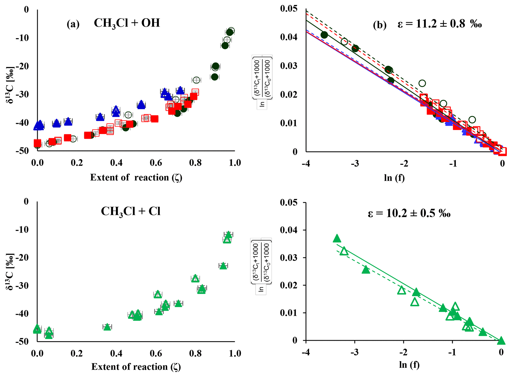
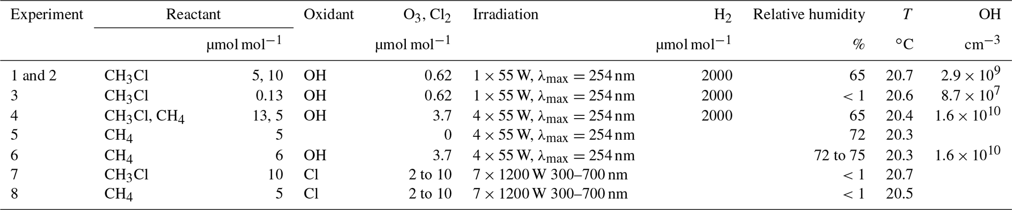
Figure 1 Change in δ¹³C over the extent of the reaction (a) and corresponding Rayleigh plots (b) from the CH₃Cl degradation experiments. Filled symbols and regression lines refer to the data from Heidelberg; open symbols and dashed regression lines show data from Hamburg. The colours refer to different degradation experiments (black is experiment 1, red is experiment 2, blue is experiment 4 and green is experiment 7). Errors in ζ were ±2 % on the 1σ level. Errors in δ¹³C, derived from the regression analysis, ranged from ±0.4 ‰ to ±1.4 ‰ on the 1σ level.

In our study, photolysis of ozone (620 nmol mol⁻¹ steady-state mixing ratio) in the absence of water vapour (relative humidity <1 %) but with 2000 µmol mol⁻¹ H₂ (experiment 3) resulted in a CH₃Cl degradation of less than 3 % over 10 h and no measurable change in the isotopic composition of CH₃Cl (−46.8 ‰ at the beginning and −46.1 ‰ after 10 h) because of the insufficient OH yield. The reaction rate constants of O(¹D) with H₂ and H₂O at 298 K are $\mathrm{1.1}\times {\mathrm{10}}^{-\mathrm{10}}$ and $\mathrm{2.2}\times {\mathrm{10}}^{-\mathrm{10}}$ cm³ s⁻¹, respectively (Burkholder et al., 2015). At a relative humidity of 70 % (corresponding to 16 000 µmol mol⁻¹), the reaction with H₂O is by far the main pathway along which OH forms (with the H₂ pathway contributing less than 4 % to the OH yield). This is consistent with the previous study, where ozone levels of 300 µmol mol⁻¹ were required for a sufficient OH production from H₂ (Gola et al., 2005; Sellevåg et al., 2006). For this experiment, the partial lifetime of CH₃Cl with respect to OH can be estimated to be about 330 h. Potential side reactions with O(¹D) were not explicitly investigated in our study but because of the reduced OH yield, this experiment allows potential losses of CH₃Cl to be constrained due to the reaction with O(¹D). In experiment 4, where both CH₃Cl and CH₄ were present, the ratio of the measured rate constants for the reaction of CH₃Cl and CH₄ with OH was 5.8. This ratio agrees well with that of the recommended rate constants of 5.6 at 298 K ($\mathrm{6.3}\times {\mathrm{10}}^{-\mathrm{15}}$ cm³ s⁻¹ for CH₄ and, $\mathrm{3.5}\times {\mathrm{10}}^{-\mathrm{14}}$ cm³ s⁻¹ for CH₃Cl at 298 K; Burkholder et al., 2015).

Table 2 Summary of the kinetic isotope effects (ε) for the reaction of CH₃Cl and CH₄ with OH and Cl from this study. We used an orthogonal regression to calculate ε and the respective uncertainties on the 1σ level for each experiment. In experiment 4 the ε for methane has not been determined.

Table 3 Compilation of kinetic isotope effects (ε) for the reaction of CH₃Cl, CH₄ and alkanes with OH and Cl.

The change in stable carbon isotope δ values of CH₃Cl (δ¹³C(CH₃Cl)) with the extent of the reaction and the corresponding Rayleigh plots of the CH₃Cl degradation experiments are shown in Fig. 1. The respective ε values, derived from the slope of the Rayleigh plot, are summarized in Table 2. For the reaction of CH₃Cl with OH, we determined an ε value of ($-\mathrm{11.2}\pm \mathrm{0.8}$) ‰ (n=3) and for the reaction with Cl we found an ε value of ($-\mathrm{10.2}\pm \mathrm{0.5}$) ‰ (n=1). The results from both laboratories generally agreed within ±1.5 ‰ (1σ) and showed no systematic difference. Variations in the initial mixing ratios (5 to 13 µmol mol⁻¹) and isotopic composition (($-\mathrm{47.0}\pm \mathrm{0.5}$) ‰ and ($-\mathrm{40.3}\pm \mathrm{0.5}$) ‰) of CH₃Cl in the OH experiments had no significant effect on the determination of the isotope effects. Furthermore, the increase in the light intensity and ozone mixing ratios in experiment 4 had no effect on the isotope effects.

The ε values for the reaction of CH₄ with OH and Cl, determined for validation purposes, agreed reasonably well with the previously published KIEs (Saueressig et al., 1995, 2001; Tyler et al., 2000; Feilberg et al., 2005). For the reaction of CH₄ with OH, we found an ε value of −4.7 ‰, which is at the upper end in terms of absolute magnitude of previously reported fractionation factors, and for the reaction with Cl we found an ε value of −59 ‰, which is more at the lower end of previously measured KIEs (Table 3). Prior to the CH₄ degradation experiment with OH, we performed a control experiment (experiment 5 in Table 1) that revealed no CH₄ loss over 10 h. With this, we can exclude any interference from reactive chlorine during the CH₄–OH experiment. The larger isotope effect for the reaction with OH found here might result from the reaction of CH₄ with O(¹D). Cantrell et al. (1990), who also used UV-photolysis in the presence of water as an OH source, reported an even higher ε value of ($-\mathrm{5.4}\pm \mathrm{0.9}$) ‰ and estimated that the reaction of CH₄ with O(¹D) (showing an ε value of −13 ‰; Saueressig et al., 2001) may have contributed about 3 % to the overall degradation. Saueressig et al. (2001) reported an ε value of −3.9 ‰ for the reaction of CH₄ with OH. With respect to this value, a contribution of 9 % from the reaction with O(¹D) is required to explain the difference in terms of O(¹D) loss.

2.3 Discussion of the CH₃Cl degradation experiments

Our newly determined isotope effects for the reaction of CH₃Cl with OH and Cl are 5 to 6 times smaller than the previously reported ε values of ($-\mathrm{59}\pm \mathrm{10}$) ‰ for the reaction with OH and of ($-\mathrm{70}\pm \mathrm{10}$) ‰ for the reaction with Cl (Gola et al., 2005). In this section, we first discuss potential sources of error in our study with particular respect to the differences between our study and the Gola study and then provide a more comprehensive comparison of our data with previous data. Gola et al. (2005) used a 250 dm³ electro polished stainless steel chamber for their degradation experiments. We used a 3500 dm³ smog chamber, made of FEP foil, for the CH₃Cl degradation experiments. The large volume of our smog chamber may result in incomplete mixing and thus in an underestimation of the KIE due to transport limitation. The effect of mixing on the observed KIE can be approximated from the timescales of mixing and reaction according to the following equation (Morgan et al., 2004; Kaiser et al., 2006):

$$\begin{array}{}\text{(3)}& {\mathit{ϵ}}_{\mathrm{obs}}\approx {\displaystyle \frac{\mathrm{1}}{\mathrm{2}}}{\mathit{\epsilon }}_{\mathrm{i}}\times \left(\mathrm{1}+\sqrt{{\displaystyle \frac{\mathrm{1}}{\mathrm{1}+Q}}}\right).\end{array}$$

Here, ε_i is the intrinsic fractionation factor, ϵ_obs is the observed fractionation factor and Q is the ratio of the mixing time and reaction timescale (1∕k). The chemical lifetime of CH₃Cl under the experimental conditions was in the order of 6 to 8 h and the turnover of air inside the chamber occurred on timescales of a few minutes. With a reaction timescale of 300 minutes and a mixing timescale of 10 min we obtain ${\mathit{\epsilon }}_{\mathrm{obs}}\approx \mathrm{0.99}\times {\mathit{\epsilon }}_{\mathrm{i}}$, making incomplete mixing an unlikely source of error. Incomplete mixing would also have affected the determination of the respective KIEs for CH₄. With those values being within previously reported ε values, we can exclude incomplete mixing as a potential source of error in our experiments. In the Gola et al. (2005) study, the mixing ratios and isotope ratios were determined with long-path FTIR. In our study, the mixing ratios were determined by GC–MS and the isotope ratios were measured by GC–IRMS in two different laboratories. Both labs used different analytical set-ups, different sampling methods and different standards. However, the results from both labs generally agree within ±1.5 ‰ on the 1σ level and show no systematic difference. As outlined before, different initial δ¹³C(CH₃Cl) as well as different initial CH₃Cl mixing ratios had no significant effect on the determination of the isotope effects. This makes analytical artefacts in our δ¹³C determination unlikely. The Cl radical generation scheme was quite similar among both studies. Gola et al. (2005) used narrowband photolysis of Cl₂, employing a Philips TLD-08 fluorescent lamp ($\mathit{\lambda }max\sim \mathrm{370}$) nm, whereas we used broadband photolysis (300 to 700 nm), making this an unlikely source for the discrepancy in between the isotope effects for the reaction of CH₃Cl with Cl.

In our study, OH was generated via UV photolysis of ozone (steady-state mixing ratios of 0.62 and 3.6 µmol mol⁻¹) in the presence of water vapour (RH of 70 %) and 2000 µmol mol⁻¹ H₂, whereas in the Gola study OH was generated in the absence of water vapour from the reaction of O(¹D) with H₂ (2000 µmol mol⁻¹) after UV-photolysis of ozone (300 µmol mol⁻¹). Due to the much lower ozone mixing ratios employed in our study, the OH generation in the absence of water vapour was not sufficient in our study. Both OH generation schemes are well established. However, Cantrell et al. (1990), who used UV-photolysis in the presence of water as an OH source, estimated that the reaction of CH₄ with O(¹D) may contribute about 3 % to the overall degradation. The higher ozone levels and the less efficient conversion of O(¹D) to OH in the Gola et al. (2005) study suggest an overall higher transient O(¹D) concentration compared to our experiments. Anyhow, interference from the reaction with O(¹D) is less likely for CH₃Cl than for CH₄. The reaction rate for CH₄ with O(¹D) $(\mathrm{1.7}\times {\mathrm{10}}^{-\mathrm{10}}$ cm³ s⁻¹; Burkholder et al., 2015) is 2.7×10⁴ times larger than the respective reaction rate for OH ($\mathrm{6.3}\times {\mathrm{10}}^{-\mathrm{15}}$ cm³ s⁻¹). In the case of CH₃Cl, the ratio is only 7.4×10³ ($\mathrm{2.6}\times {\mathrm{10}}^{-\mathrm{10}}$ and $\mathrm{3.5}\times {\mathrm{10}}^{-\mathrm{14}}$ cm³ s⁻¹; Burkholder et al., 2015). Assuming a contribution of 9 % from the reaction with O¹D in the CH₄ experiment, the reaction with O(¹D) should contribute less than 2.3 % to the observed CH₃Cl loss. In the CH₃Cl control experiment, all experimental parameters besides the relative humidity and hence the OH yields were comparable to CH₃Cl degradation experiments with OH. The CH₃Cl loss of less than 3 % over 10 h can most likely be attributed to a reaction with OH, originating from the reaction of O(¹D) with H₂. The δ¹³C values of CH₃Cl were −46.8 ‰ at the beginning and −46.1 ‰ after 10 h, which are indistinguishable within the measurement uncertainty. This experiment makes any biasing side reactions unlikely. In any case we can limit the loss from potential side reactions to less than 3 %. In addition, none of our tests prior each degradation experiment revealed an indication of a measurable loss of CH₃Cl. With this, we can safely exclude any measurable effect from potential side reactions on the determination of the KIEs in our study.

A comparison of our data with previously measured and calculated isotope effects for the reaction of CH₃Cl, CH₄ and other VOCs with OH and Cl is provided in Table 3. In a follow-up study to Gola et al. (2005), Sellevåg et al. (2006) attributed these exceptionally large fractionation factors to higher internal barriers of rotation of the OH radical compared to the CH₄+OH reaction. Using variational transition state theory, the authors calculated ε values of −47 ‰ and −37 ‰ for the reaction of CH₃Cl with OH and Cl, respectively. However, a simultaneous theoretical study provided an ε value of only −3.6 ‰ for the reaction of CH₃Cl with OH (Jalili and Akhavan, 2006). For C–H bond breakage, Streitwieser's semi-classical limit for isotope effects is −21 ‰ (Elsner et al., 2005), and for reactions involving hydrogen radical transfer, an ε value of −15 ‰ has been reported (Merrigan et al., 1990). Both values support a lower fractionation factor. For the reaction of ethane with OH, which can be approximately regarded as a substituted methane, an ε value of ($-\mathrm{7.5}\pm \mathrm{0.5}$) ‰ has been reported (Piansawan et al., 2017). One can estimate an upper limit for the reactive site by multiplying δ¹³C with the number of carbon atoms in the molecule (Anderson et al., 2004). This leads to an upper limit of ($-\mathrm{15.0}\pm \mathrm{0.7}$) ‰ for the ε value at the reactive centre. In line with this, Anderson et al. (2004) reported a group kinetic isotope effect of ($-\mathrm{18.7}\pm \mathrm{5.2}$) ‰ for the reaction of primary carbon atoms of alkanes with OH. The same group (Anderson et al., 2007) found a group kinetic isotope effect of ($-\mathrm{18.6}\pm \mathrm{0.3}$) ‰ for the respective reaction with Cl. Our smaller kinetic isotope effect for the reaction of CH₃Cl with OH and Cl is much closer to these group-specific kinetic isotope effects than the previously reported ones from Gola et al. (2005).

To this end, the large discrepancy between our data and those of Gola et al. (2005) remains unresolved and cannot be explained from experimental details. However it appears that the authors have not tested the accuracy of their isotope ratio measurements as a function of the isotopologue mole fraction in the presence of other species with overlapping spectra (HCl, H₂O, O₃, etc.), e.g. by using a dilution series.

In any case, the strongest support for our smaller isotope effects arises from the absence of any significant seasonal variation in the tropospheric δ¹³C(CH₃Cl), as shown in Sect. 3.5.

3 Carbon isotope modelling

3.1 Model set-up

The model used in this study is similar to previous two box models (Tans, 1997; Sapart et al., 2012; Saltzman et al., 2004; Trudinger et al., 2004). The atmosphere is divided in two well-mixed semi-hemispheric boxes, representing the Northern and the Southern Hemisphere, and the interhemispheric exchange time is 360 days. The model simulates the major sources and sinks for both the lighter (¹²CH₃Cl) and the heavier isotopologue (¹³CH₃Cl), as described by Sapart et al. (2012) for CH₄. The source and sink terms from the Xiao et al. (2010) model study serve as a starting point for our model. We use a simplified mass balance with four source categories that has distinct isotopic source signatures: higher plants/unknown, oceans, biomass burning and other known sources (Sect. 3.3 and Table 4). Total net emissions were fixed at 4010 Gg a⁻¹ with 2210 Gg a⁻¹ in the Northern Hemisphere and 1800 Gg a⁻¹ in the Southern Hemisphere. For each source category, the carbon isotope source signature was randomly varied within the given uncertainties (Table 4). Losses are specified by pseudo first-order rate coefficients. The sinks implemented in the model (Sect. 3.4 and Table 4) are losses due to the reaction with OH, losses to the surface ocean, losses to soils and losses to the stratosphere. Seasonal variations were modelled with a time step of 1 day, using monthly averaged source terms. Variations in the source composition were modelled with a time step of 90 days, using annually averaged source terms.

Table 4 Simplified CH₃Cl source and sink scheme used in the model.

^∗ The apparent isotope effect of the soil sink depends on its strength. See text for more details.

3.2 Mixing ratios and isotopic composition of tropospheric CH₃Cl

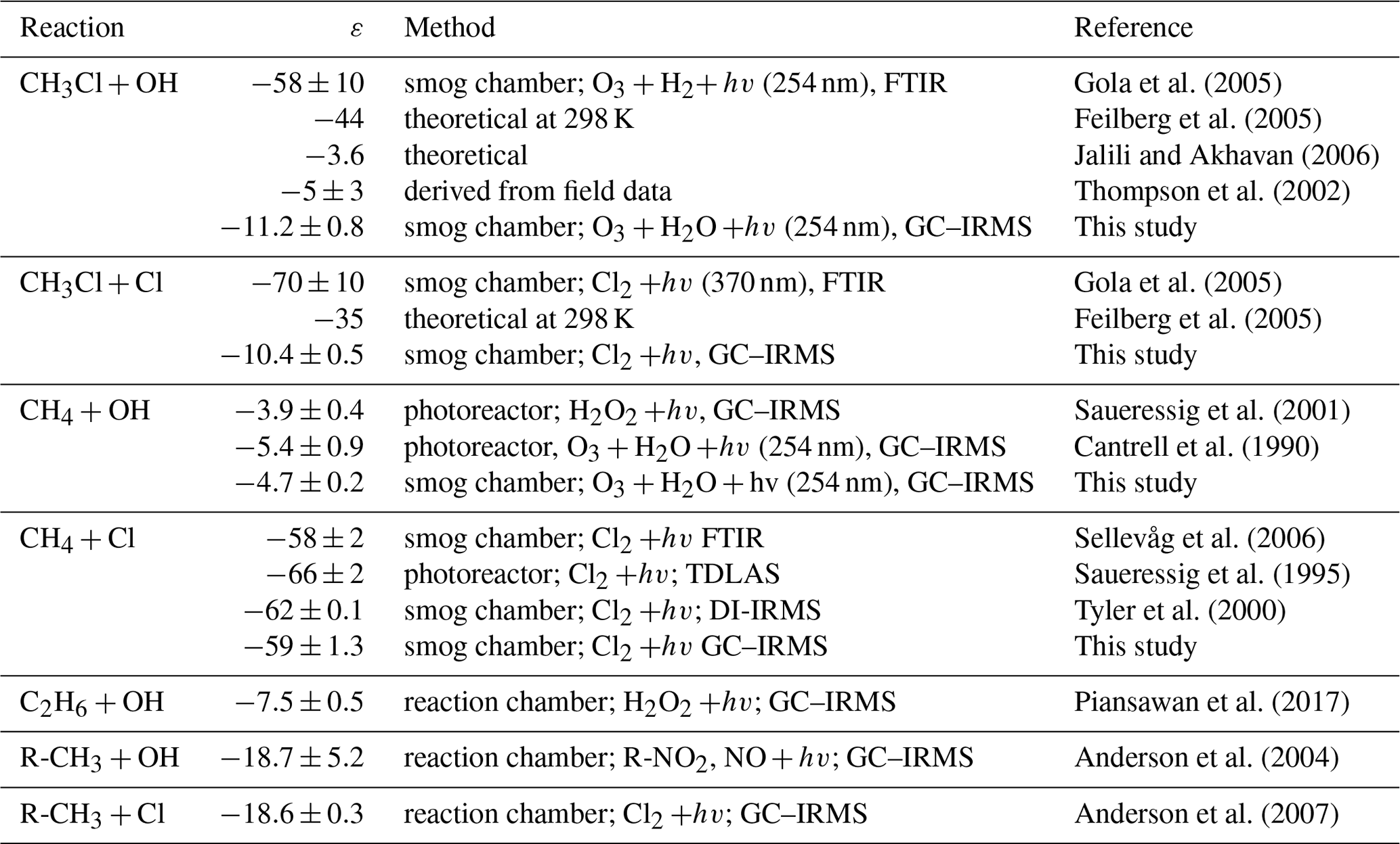
Tropospheric CH₃Cl has a mean global mixing ratio of about 540 pmol mol⁻¹ (Monzka et al., 2010; Carpenter et al., 2014) and shows a pronounced seasonal cycle with an amplitude of 85 pmol mol⁻¹ at Northern Hemispheric midlatitudes, (Prinn et al., 2000; Yoshida et al., 2006), reflecting the seasonality in the OH sink (Fig. 2, upper panel).

Figure 2 (a) Comparison of modelled northern hemispheric mixing ratios (blue open diamonds) with measured mixing ratios at Mace Head, Ireland (red crosses) for the period from 2004 to 2014 (Prinn et al., 2000). Error bars indicate the variations in the monthly means on the 1σ level. (b) Modelled seasonal fluctuations in the δ¹³C of northern hemispheric CH₃Cl using an ε of −11.2 ‰ (red filled diamonds) and an ε of −59 ‰ (blue filled dots) as reported by Gola et al. (2005). The panel shows monthly averages from a 10-year simulation with seasonal variations of up to ±10 ‰ in the combined isotopic source signature. Error bars indicate the variations in the monthly means on the 1σ level. The grey shaded area shows reported seasonal variations (seasonal mean ±1σ) from Thompson et al. (2002).

Reported mean δ¹³C values of tropospheric CH₃Cl range from ($-\mathrm{36.2}\pm \mathrm{1.9}$) ‰ to ($-\mathrm{40.8}\pm \mathrm{3.0}$) ‰ (Tsunogai et al., 1999; Thompson et al., 2002; Redeker et al., 2007; Bahlmann et al., 2011; Weinberg et al., 2014), suggesting an overall mean δ¹³C(CH₃Cl) of ($-\mathrm{37.1}\pm \mathrm{2.7}$) ‰. In a year-round study carried out in Alert, Canada, Thompson et al. (2002) found no seasonal trend in the tropospheric δ¹³C(CH₃Cl) and no clear correlation between the CH₃Cl mixing and isotope ratios (Fig. 2, lower panel). From their data the authors estimated the ε value for the OH sink at less than −5 ‰. Including samples from Frazer Point (Canada), Vancouver (Canada), Houston (Texas, USA) and Barring Head (New Zealand), this study further revealed no indication of a latitudinal trend in tropospheric δ¹³C(CH₃Cl). The lack of a significant covariation between the mixing ratios and carbon isotope ratios was confirmed in a second year-round study (Redeker et al., 2007).

3.3 Sources

The seasonal source terms are specified for each hemisphere using monthly means as depicted in Fig. 3. The ocean is treated as a net source for CH₃Cl with an annual net emission of 335 Gg a⁻¹ (range: 80 to 610 Gg a⁻¹) (Hu et al., 2013). To account for the bidirectional nature of the gas exchange across the air–sea interface, net fluxes are broken down into unidirectional gross uptake and emission fluxes, with the uptake carrying the isotopic composition of the atmosphere and the emission carrying the isotopic information of the concurrent formation and degradation processes in the ocean. The gross uptake is calculated using an average transfer velocity of 17 cm h⁻¹ for CO₂ (Wanninkhof, 2014) and a mean tropospheric mixing ratio of 540 pmol mol⁻¹. Gross emissions are then calculated as the difference between net emissions and gross uptake fluxes. The reader should note that this approach differs from that of Hu et al. (2013) and results in larger gross fluxes because gross fluxes are calculated for the entire ocean surface. Keppler et al. (2005) estimated average isotopic composition of dissolved CH₃Cl to ($-\mathrm{36}\pm \mathrm{4}$) ‰. This value refers to Komatsu et al. (2004), who reported a mean δ¹³C of −38 ‰ for CH₃Cl in coastally influenced waters off Japan and more enriched δ¹³C values in the range of −12 ‰ to −30 ‰ from the open north-eastern Pacific. We obtained average δ¹³C values of $-\mathrm{43}\pm \mathrm{3}$ ‰ from a productive lagoon in southern Portugal (Weinberg et al., 2015). Taking the biotic and abiotic degradation of CH₃Cl into account, we estimate the mean isotopic source signature of the ocean source to be ($-\mathrm{36}\pm \mathrm{6}$) ‰.

Figure 3 Chloromethane emissions in Gg month⁻¹ for the Northern (a, c, e, g) and Southern Hemisphere (b, d, f, h). (a, b) Combined emissions from higher plants and the unknown source, (c, d) biomass burning, (e, f) ocean net emission fluxes, and (g, h) total emissions. The emissions from the other known sources are constant over time, with 22.8 Gg month⁻¹ in the Northern Hemisphere and 7.6 Gg month⁻¹ in the Southern Hemisphere.

We applied a source strength of 910 Gg a⁻¹ for biomass burning (range from 660 to 1230 Gg a⁻¹) with 68 %, originating from the Northern Hemisphere, and the emissions peaking during hemispheric spring (Xiao et al., 2010). CH₃Cl from biomass burning shows a δ¹³C of ($-\mathrm{47}\pm \mathrm{7}$) ‰ (Czapiewski et al., 2002; Thompson et al., 2002).

The category “other known sources” comprises fungi wetlands and anthropogenic emissions with a total source strength of 365 Gg a⁻¹ (range: 79 to 1016 Gg a⁻¹) and an averaged isotopic source signature of ($-\mathrm{45.5}\pm \mathrm{5.5}$) ‰ calculated from the source signatures given by Keppler et al. (2005). The emissions from the other known sources were constant over time with 274 Gg a⁻¹ in the Northern Hemisphere and 91 Gg a⁻¹ in the Southern Hemisphere.

The source category “higher plants/missing” (900 to 3095 Gg a⁻¹) mainly represents emissions from the tropical rainforest (900 to 2650 Gg a⁻¹) with minor contributions from salt marshes (80 to 160 Gg a⁻¹), rice paddies (5 Gg a⁻¹) and mangroves (∼50 Gg a⁻¹). These emissions are almost equally distributed between the hemispheres and show a slight seasonal peak during hemispheric summer. In order to evaluate the emissions from higher plants, these emissions were divided into two fractions by introducing a split factor. The first fraction represents “true” emissions from higher plants, having an exceptionally depleted isotopic source signature of ($-\mathrm{83}\pm \mathrm{15}$) ‰ (Saito and Yokouchi, 2008; Saito et al., 2008). The second fraction represents an unknown or missing source. The δ¹³C of this source is scaled to match the δ¹³C of tropospheric CH₃Cl. A more depleted δ¹³C for this source would point towards additional contributions from a lighter source, such as senescent leaf litter, whereas a more enriched δ¹³C for this source points towards additional contributions from a more enriched source.

Saito et al. (2013) recently reported on the bidirectional exchange of CH₃Cl across the leaves of tropical plants with gross uptake rates being roughly a sixth of gross emission rates. The authors hypothesized that the gross uptake may be related to endosymbiotic bacteria. This uptake might affect the isotopic composition of CH₃Cl from tropical rainforests. However, because the incubation methods used in this study were the same as those previously used to determine the isotopic composition of CH₃Cl emitted from tropical plants (Saito and Yokouchi, 2008; Saito et al., 2008), we can reasonably assume that any potential isotopic effect of this bidirectional exchange is included in the previously reported carbon isotope ratios.

3.4 Sinks

The reaction with OH constitutes the single largest sink for CH₃Cl, accounting for approximately 80 % of its removal from the troposphere. For this study, we used the OH-concentration fields from Spivakovsky et al. (2000) along with reaction rate constants of Burkholder et al. (2015) to derive monthly resolved lifetimes for both hemispheres. The monthly loss rates were then forced to reproduce seasonal variations of the mixing ratios at Mace Head in the Northern Hemisphere and at Cape Grim, Tasmania, in the Southern Hemisphere (Prinn et al., 2000). This resulted in a total tropospheric sink (OH + Cl) of 3614 Gg a⁻¹, which is comparable to previous modelling studies (Xiao et al., 2010).

In most global budgets, soils are treated as a small sink for chloromethane of about ∼250 Gg a⁻¹, though a larger uptake exceeding 1000 Gg a⁻¹ has been suggested (Keppler et al., 2005; Carpenter et al., 2014). Based on Xiao et al. (2010), we a priori assumed a soil sink of 250 Gg a⁻¹ with northern and southern hemispheric fractions of 180 and 70 Gg a⁻¹, reflecting the interhemispheric distribution of the land masses.

The microbial degradation of CH₃Cl in soils is assigned with a large carbon isotope effect of −47 ‰ (Miller et al., 2001, 2004). The only study we are aware of (Redeker and Kalin, 2012) that investigates the isotopic composition of soil derived CH₃Cl reports a δ¹³C of ($-\mathrm{34}\pm \mathrm{14}$) ‰. The soil uptake of CH₃Cl can be regarded as a coupled diffusion reaction process, where CH₃Cl is first transported into the soil and then undergoes microbial degradation. The apparent isotope effect of such coupled processes will depend on the isotope effects of both steps and can be estimated from diffusion reaction models (Farquhar et al., 1982):

$$\begin{array}{}\text{(4)}& {\mathit{\epsilon }}_{\mathrm{app}}={\mathit{\epsilon }}_{\mathrm{d}}+{\displaystyle \frac{\left({\mathit{ϵ}}_{\mathrm{m}}-{\mathit{\epsilon }}_{\mathrm{d}}\right)\times (m_{\mathrm{d}}-m_{\mathrm{m}})}{m_{\mathrm{d}}}},\end{array}$$

with ε_d and ε_m being the kinetic isotope effects assigned to microbial degradation (47 ‰) and diffusion (4 ‰), and where m_d is the total mass of CH₃Cl that enters the soil via diffusion and m_m represents the net soil sink.

The gross uptake flux (m_d) was estimated using a simple transfer resistance model along with the biomes and respective active seasons as previously employed by Shorter et al. (1995). We used an overall atmospheric transfer resistance governing the transport to the soil surface (aerodynamic transport resistance, quasi-laminar sublayer resistance and in canopy transfer resistance) of 4 s cm⁻¹, regardless of the biome, that was derived from reported typical transfer resistances for different biomes (Zhang et al., 2003). The soil uptake is governed by molecular diffusion through the air-filled pore space. The soil-side transfer resistance can be estimated from the effective diffusion in the soil column. For a first rough estimate of the soil transfer resistance, we assume an air-filled pore space of 0.3 (V∕V) and a microbial inactive soil layer of 0.5 cm at the soil surface. Using the Penman model (Penman, 1940) and a diffusion coefficient of 0.144 cm² s⁻¹ in air, we obtain a soil transfer resistance of 17 s cm⁻¹. With a globally averaged transfer resistance of 21 s cm⁻¹ and a CH₃Cl background concentration of 540 pmol mol⁻¹ and the land use categories from Shorter et al. (1995), we obtain an upper limit of 1300 Gg a⁻¹ for m_d.

As depicted in Fig. 4, the apparent isotope effect of the soil uptake is bracketed by the isotope effects of both steps and decreases when increasing the net soil uptake. The microbial degradation is rate limiting at low net uptake rates, and the apparent isotope effect of the soil uptake is close to that for microbial degradation. For instance, a soil sink of 250 Gg a⁻¹ reveals an apparent ε value of −38 ‰. When the entire chloromethane diffusing into soils is microbially degraded, diffusion becomes the rate-limiting step, and the apparent ε value matches that of diffusion.

In turn the imprint on the tropospheric δ¹³C shows a parabolic distribution with a maximum at m_m=0.5 m_d. The isolated effect of the soil sink would result in a maximum enrichment of 3.8 ‰ in the tropospheric δ¹³C that reduces to 2.1 ‰ when accounting for the concurrent reduction in the OH sink. In this case, increasing the soil sink could even lead to a decrease in the overall sink isotope effect once the apparent isotope effect of the soil sink becomes smaller than the isotope effect of the OH sink.

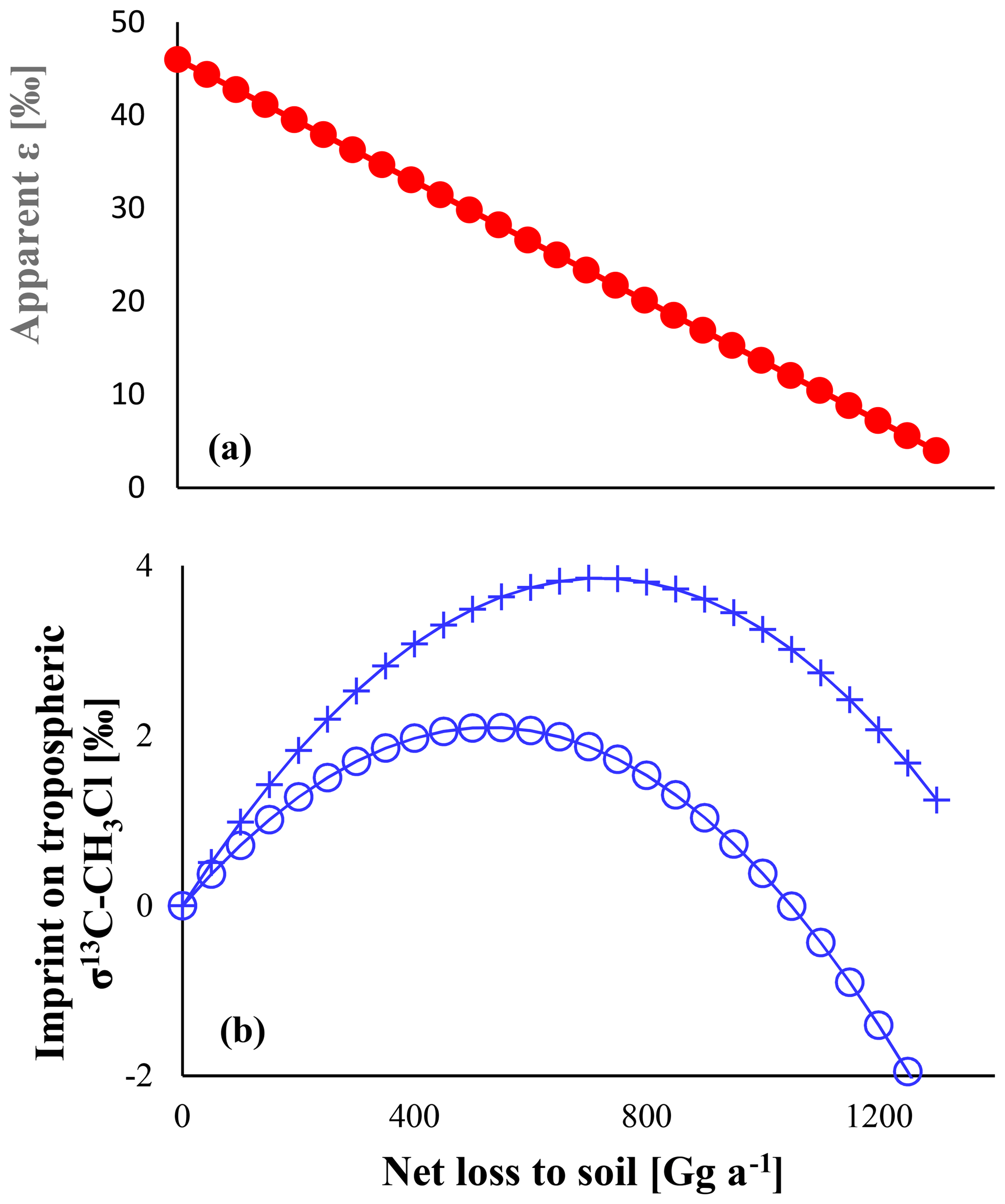
Figure 4 Panel (a) shows the apparent ε of the soil sink versus the sink strength. Panel (b) shows the resulting effect on tropospheric δ¹³C. Crosses show the pure effect, e.g. in the absence of any other fractionating sink. Open circles show the resulting effect with an ε of −11.2 ‰ assigned to the OH sink. Total losses were assumed to be fixed at 4010 Gg a⁻¹.

3.5 Seasonal variations in the δ¹³C of tropospheric CH₃Cl

The OH-driven seasonal cycle in the tropospheric mixing ratios of CH₃Cl implies an inverse covariation in the δ¹³C of tropospheric CH₃Cl to an extent that is closely linked to the kinetic isotope effect of the OH sink.

Our model resembles mean tropospheric mixing ratios of about 540 pmol mol⁻¹ (Monzka et al., 2010; Carpenter et al., 2014) and the seasonal cycles of CH₃Cl in both hemispheres within ±4 % (Fig. 2 upper panel). In our simulations, an ε value of −59 ‰ for the OH sink produces an inverse covariation of the δ¹³C(CH₃Cl) with the CH₃Cl mixing ratios with a seasonal amplitude of 9.2 ‰, whereas our new smaller ε value of −11.2 ‰ results in a seasonal amplitude of only 1.7 ‰ (Fig. 2 lower panel), fitting quite well to the measured variation given by Thompson et al. (2002).

Random variations of ±10 ‰ in the isotopic source signatures, seasonal variations of the emission functions and variations in the soil sink resulted in seasonal fluctuations of up to ±10 ‰ in the combined isotopic source signature (see Supplement for further details). As already noted by Tans (1997) the large tropospheric background strongly attenuates temporal variations. In our model simulations these seasonal variations in the combined isotopic source signature resulted in systematic seasonal variations of the northern hemispheric δ¹³C of less than ±0.7 ‰ attributable to the isotopic source signal and a scatter of up to ±1.0 ‰ in the monthly mean δ¹³C(CH₃Cl) values in the Northern Hemisphere. In all our model simulations these variations in the combined isotopic source did not significantly affect the differences in the seasonal amplitude of the tropospheric δ¹³C signal. They may have an imprint on the tropospheric δ¹³C(CH₃Cl) signal when applying an ε value of −11.2 ‰ to the OH sink. However, they are largely obscured when applying an ε value of −59 ‰ to the OH sink (Fig. S6 in the Supplement). Masking the isotope effect of this large ε value would require seasonal variations of about 50 ‰ in the combined source signatures that are inversely correlated to the OH sink. In sum, the lacking covariation between the mixing ratios and carbon isotope ratios strongly supports our new ε value of −11.2 ‰ and makes the previously reported larger ε value highly unlikely.

3.6 Implications for the tropical rainforest source

An ε value of −59 ‰ for the OH sink requires a mean mass-weighted isotopic source composition of −84.5 ‰ to balance the tropospheric δ¹³C(CH₃Cl) of ($-\mathrm{36.4}\pm \mathrm{2.1}$) ‰ (Thompson et al., 2002), as shown in previous studies. Apart from large emissions from higher plants (Keppler et al., 2005; Saito and Yokouchi, 2008) in tropical rainforests, this isotope effect suggests additional substantial emissions from an even more depleted source, such as senescent leaf litter (Keppler et al., 2005; Saito and Yokouchi, 2008). In contrast, the revised smaller ε value of −11.2 ‰ requires a mean isotopic source signature of −48.5 ‰, which is close to the mass-weighted δ¹³C of all other known sources excluding higher plants. Along with higher plant emissions of 2200 Gg a⁻¹, the new ε value of −11.2 ‰ yields a mean tropospheric δ¹³C(CH₃Cl) of −56 ‰, which is depleted by almost 20 ‰ in comparison to the mean reported tropospheric δ¹³C(CH₃Cl).

We performed more than 10 000 steady-state runs with random variations in the isotopic composition of tropospheric CH₃Cl ($-\mathrm{36.4}\pm \mathrm{2.1}$ ‰), the isotopic source signatures (Table 4) and the isotope effect of the soil sink to assess the range of CH₃Cl emissions from higher plants. The source category “higher plants” was divided in two fractions, one representing “true” emissions from higher plants and the other representing missing emissions. The δ¹³C of the missing emissions was always scaled to match the tropospheric δ¹³C(CH₃Cl).

As shown in Fig. 5, the strength of the tropical rainforest source is directly linked to the strength and isotopic composition of missing emissions. A tropical rainforest source of (600±200) Gg a⁻¹ suggests missing emissions of (1600±200) Gg a⁻¹, requiring a δ¹³C of ($-\mathrm{45}\pm \mathrm{6}$) ‰ to balance the tropospheric δ¹³C(CH₃Cl). This δ¹³C is close to the mean isotopic composition of all other known sources. Increasing the emissions from all other known sources within the given ranges might reduce the missing emissions by about 500 Gg a⁻¹. A further increase of the tropical rainforest emissions results in an equivalent reduction in missing emissions but requires a more enriched δ¹³C for the missing emissions. For instance, balancing a tropical rainforest source of (1100±200) Gg a⁻¹ requires missing emissions of the same magnitude with a δ¹³C of ($-\mathrm{31}\pm \mathrm{6}$) ‰. This is at the upper end of reported source signatures and may thus serve as a boundary with which to constrain the rainforest source from an isotopic perspective.

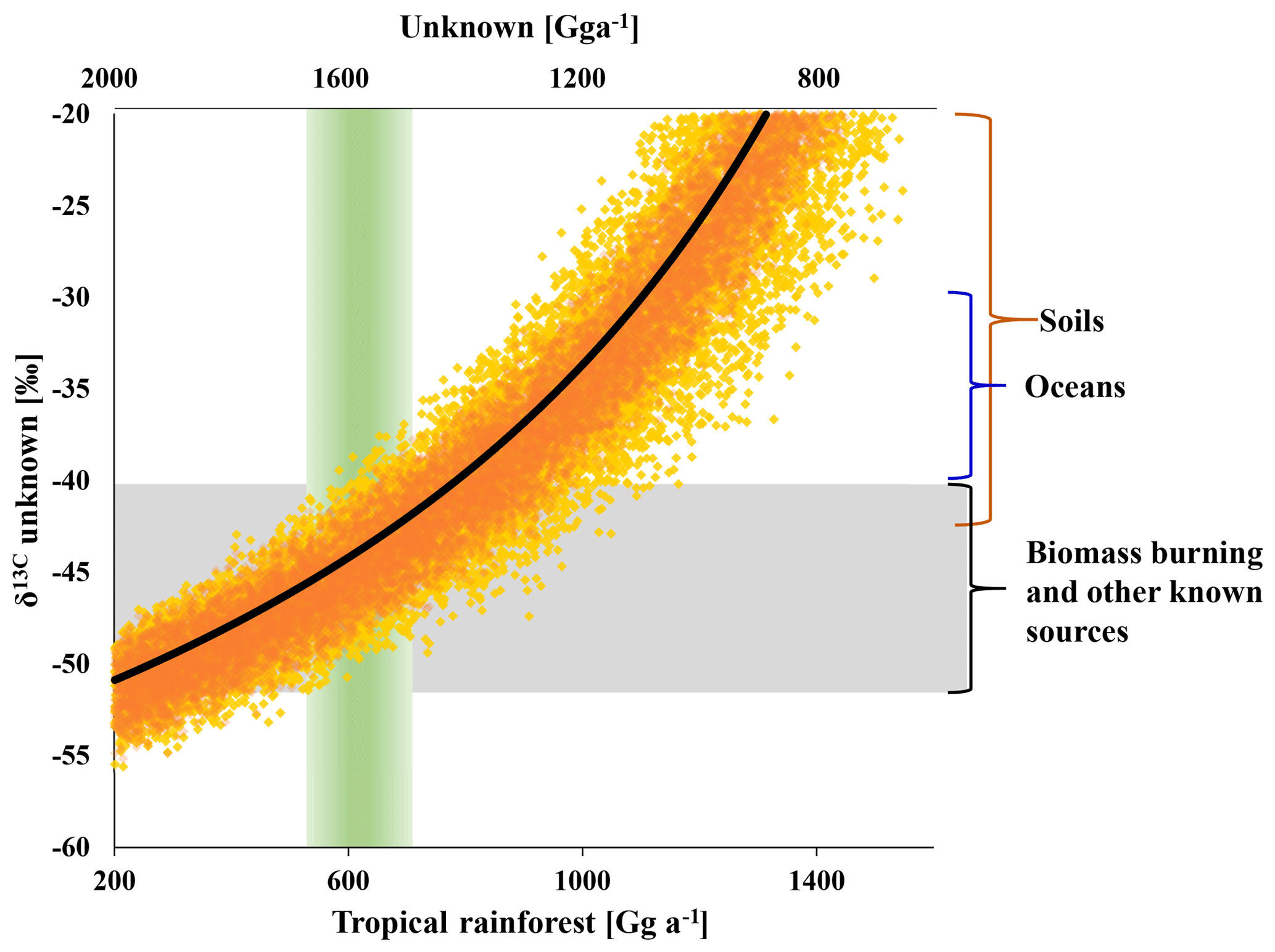
Figure 5 Modelled isotopic composition of the missing source versus tropical rainforest emissions on the lower x axis and missing emissions on the upper x axis (rainforest = 2200 – unknown). The black line shows the best estimate derived from the mean isotopic source signatures. Orange dots indicate the range uncertainty (1σ) from uncertainties (1σ) in the δ¹³C of biomass burning (±7 ‰), ocean net emissions (±6 ‰) and other known sources (±6 ‰). Yellow dots mark the additional uncertainty from the δ¹³C of the tropical rainforest source (±10 ‰). The green column indicates the carbon-density-based estimate of the rainforest source and the grey bar indicates the range in δ¹³C of biomass burning and the mean from all sources excluding the tropical rainforest.

4 Carbon-density-based revision of the tropical rainforest source

Interestingly, support for our lower estimate arises from previous studies on the tropical rainforest CH₃Cl source when using above-ground carbon density instead of coverage area for upscaling the CH₃Cl emission factors.

Large uncertainties in upscaling of locally derived plant emissions to global scales can arise from (i) temporal variations in the emissions and (ii) spatial variability in environmental drivers, species composition and vegetation cover. Within the widely used FAO land cover classes, forests are defined as land with tree cover exceeding 10 %, a potential tree height of 5 m and an area of at least 0.5 ha (FAO, 2012). Tropical rainforests encompass such sparsely covered areas with a carbon density of only a few Mg ha⁻¹ (Asner et al., 2010; Pereira et al., 2016) as well as very dense mature rainforests with a canopy height of more than 40 m and above-ground carbon densities sometimes exceeding 300 Mg ha⁻¹ (Kato et al., 1978). This suggests a large variability in biomass that cannot be assessed with the previously used area-based upscaling approaches. Area-based estimates may be improved by leaf area index or above-ground carbon-density-based approaches. There is some indication that CH₃Cl is mainly emitted by mature trees (Saito and Yokouchi, 2008; Saito et al., 2008, 2013). This is more readily reflected by carbon density than by leaf area. Further, the available carbon density data products allow direct discrimination between tropical forests and other tropical vegetation. We thus propose a carbon-density-based upscaling approach of experimentally derived emission factors to reduce uncertainties arising from the spatial variability in above-ground biomass. We first convert reported area-based emission factors to carbon-density-based emission factors and then multiply them with the carbon stock of the tropical rainforest:

$$\begin{array}{}\text{(5)}& F\left({\mathrm{CH}}_{\mathrm{3}}\mathrm{Cl}\right)={\displaystyle \frac{E_F\times C_{\mathrm{RF}}}{C_{\mathrm{st}}}}.\end{array}$$

Here, F(CH₃Cl) is the source strength [Gg a⁻¹], E_F is the experimentally derived emission factor [Gg ha⁻¹ a⁻¹], C_st is the above-ground carbon density assigned to the sampling site [Gg ha⁻¹] and C_RF is the estimated total above-ground biomass [Gg] of the respective biome, in this case the tropical rainforest.

Table 5 Calculation of carbon-density-based CH₃Cl emission factors from previously reported area-based emission factors.

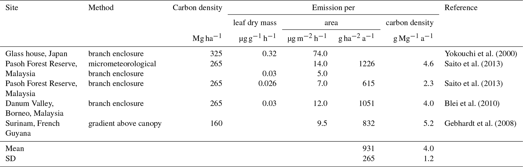
The first direct evidence for strong CH₃Cl emissions from tropical plants came from branch incubations of tropical plants in a greenhouse (Yokouchi et al., 2000). This study revealed particularly high emission from dipterocarp species that are dominant in tropical lowland rainforests of southern and south-eastern Asia and suggested mean CH₃Cl emissions of 74 µg m² h⁻¹. Several follow-up studies carried out in tropical rainforests reported 10- to 5-fold lower fluxes (Saito et al., 2008, 2013; Gebhardt et al., 2008; Blei et al., 2010). We exclude the high-emission factor from the greenhouse study from our reanalysis of the tropical rainforest source and focus on the studies, providing experimentally derived emission factors for CH₃Cl emissions from tropical forests and allowing for a sufficient estimate of carbon densities assignable to them. Details on these studies are provided in Table 5. Three studies have been carried out in lowland tropical rainforests of south-eastern Asia, and one has been carried out over Surinam in South America. We are not aware of any CH₃Cl flux measurements from African tropical rainforests. Two studies relied on branch or leaf incubation to measure CH₃Cl fluxes (Saito et al., 2013; Blei et al., 2010). A third study used a micrometeorological approach and in addition performed leaf and branch incubation (Saito et al., 2008). The remaining study (Gebhardt et al., 2008) derived CH₃Cl emissions factors from concentration gradients above the rainforest. The concentration gradients were obtained from canister samples taken at different heights above the rainforest from an airplane. The results from branch and leaf incubations were first normalized to leaf dry weight and then converted to area-based emission factors using reported allometric data for south-eastern Asian tropical lowland rainforests along with assumptions of the distribution and abundance of the investigated species. The mean area normalized fluxes (8.0 µg m² h${}^{-\mathrm{1}}\pm \mathrm{45}$ %) from these studies show a notably larger variability than the original leaf biomass normalized fluxes (0.028 µg g⁻¹ h${}^{-\mathrm{1}}\pm \mathrm{10}$ %), although all three studies referred to the same allometric data (Yamakura et al., 1986) in their conversion. Note that the study reporting the lowest emissions factors from branch enclosures reported almost 3 times higher fluxes using a micrometeorological approach. In sum, the area-based factors agree within a factor of 3 and range from 5.0 to 14 µg m² h⁻¹ (9.1 µg m² h${}^{-\mathrm{1}}\pm \mathrm{37}$ %).

Table 6 Comparison of calculated area-based and carbon-density-based emissions from tropical forests.

¹ Saatchi et al. (2011); ² Baccini et al. (2012).

The three south-eastern Asian studies refer to a dense and mature dipterocarp forest with an above-ground carbon density of (265±44) Mg C ha⁻¹ (Yamakura et al., 1986) that we apply here. For the study carried out above the rainforest of Surinam, we derived a carbon density of (160±15) Mg ha⁻¹ from carbon density maps (Saatchi et al., 2011; Baccini et al., 2012).This range agrees with the FAO estimate for French Guyana (FAO, 2015) and is supported by several field surveys carried out in this region (Chave et al., 2001, 2008; Saatchi et al., 2007). With this, we obtain a mean carbon-density-based emission factor of (4.0±1.2) g Mg⁻¹, referring to a mean carbon density of 202 Mg ha⁻¹. This is well above the average tropical rainforest carbon density, ranging from 96 to 117 Mg ha⁻¹ (Baccini et al., 2012; Saatchi et al., 2011; Köhl et al., 2015; FAO, 2015).

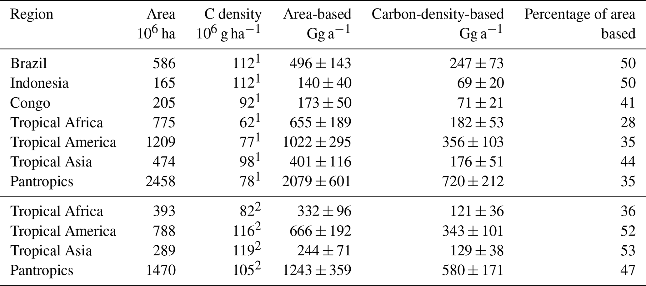
In consequence, our carbon-density-based estimates of the tropical CH₃Cl source are 30 % to 70 % lower than the respective area-based estimates (Table 6). The difference is in the range of 30 % for dense old grown evergreen forests such as the Tierra Firme forests of French Guyana, between 40 % and 50 % for the moist tropical rainforest, and increases to almost 70 % for the entire pantropical forests including dry tropical forests, degraded forests and plantations. This trend reflects the decreasing trend in carbon density in the tropical rainforest biomes as well as the effect of forest degradation. Regardless of the source for the carbon density estimates, our approach suggests a tropical rainforest CH₃Cl source of (670±250) Gg a⁻¹, which is 53 % to 65 % lower than the respective area-based estimates in the range of 1200 to 2000 Gg a⁻¹ (Saito et al., 2008, 2013; Gebhardt et al., 2008; Blei et al., 2010).

The uncertainty in the area-based emission factors is estimated to 24 % from the standard deviation of the reported means. Additional uncertainties for our carbon-density-based upscaling (compared to the previous area-based upscaling) arise from the uncertainties in the total above-ground carbon stocks (±8.6 %) and the site-specific carbon density (±15 %). Using error propagation, we estimate the total uncertainty of our approach to be ±30.4 %. However, we note an urgent need for more detailed flux studies. Currently there is no information about how physiological and environmental drivers might affect CH₃Cl emissions from tropical rainforests. Apart from the observation that some members of the Dipterocarpaceae family are particularly strong emitters of CH₃Cl, this also holds true with respect to species composition.

5 Conclusions

We reported new ε values for the reaction of CH₃Cl with OH and Cl of ($-\mathrm{11.2}\pm \mathrm{0.8}$) ‰ (n=3) and ($-\mathrm{10.2}\pm \mathrm{0.5}$) ‰, which are 5 to 7 times smaller than the previously reported ε values for these reactions. Strong support for the reliability of our new fractionation factors arises from the absence of any significant covariation in the mixing and carbon isotope ratios of tropospheric CH₃Cl.

Conjoining our new KIEs of the tropospheric CH₃Cl sinks and the biomass-based upscaling of previously reported emission factors suggests a tropical vegetation source of only (670±200) Gg a⁻¹, which is about 3-fold smaller than suggested in current budgets. We assign δ¹³C of $-\mathrm{45}\pm \mathrm{6}$ ‰ to the missing emissions of (1530±200) Gg a⁻¹. Notably increasing the soil sink by 750 Gg a⁻¹ and decreasing biomass burning emissions by 460 Gg a⁻¹, as suggested in the latest assessment on ozone-depleting substances (Carpenter et al., 2014), would substantially increase this gap but have a negligible effect on the isotopic composition of the missing emissions. The δ¹³C value of the missing emissions matches with the mean source signature of the other known sources (except rainforests). Increasing these emissions within the given ranges might reduce the gap to (1100±200) Gg a⁻¹. From a purely isotopic perspective, in particular larger emissions from biomass burning could further reduce this gap. However, this is highly speculative as virtually any source combination providing a mean δ¹³C of $-\mathrm{45}\pm \mathrm{6}$ ‰ could fill the gap.

With CH₃Cl being the single largest natural carrier of chlorine to the stratosphere, predicting future baselines of stratospheric chlorine requires a better understanding of the global CH₃Cl cycle and an identification of the missing emissions.