the Creative Commons Attribution 4.0 License.
the Creative Commons Attribution 4.0 License.
 | 17 Dec 2019
Inferring the anthropogenic NOx emission trend over the United States during 2003–2017 from satellite observations: was there a flattening of the emission trend after the Great Recession?
Jianfeng Li
We illustrate the nonlinear relationships among anthropogenic NOx emissions, NO2 tropospheric vertical column densities (TVCDs), and NO2 surface concentrations using model simulations for July 2011 over the contiguous United States (CONUS). The variations in NO2 surface concentrations and TVCDs are generally consistent and reflect anthropogenic NOx emission variations for high anthropogenic NOx emission regions well. For low anthropogenic NOx emission regions, however, nonlinearity in the anthropogenic-emission–TVCD relationship due to emissions from lightning and soils, chemistry, and physical processes makes it difficult to use satellite observations to infer anthropogenic NOx emission changes. The analysis is extended to 2003–2017. Similar variations in NO2 surface measurements and coincident satellite NO2 TVCDs over urban regions are in sharp contrast to the large variation differences between surface and satellite observations over rural regions. We find a continuous decrease in anthropogenic NOx emissions after 2011 by examining surface and satellite measurements in CONUS urban regions, but the decreasing rate is lower by 9 %–46 % than the pre-2011 period.
- Article
(8832 KB) - Full-text XML
-
Supplement
(1476 KB) - BibTeX
- EndNote


Anthropogenic emissions of nitrogen oxides (NOx = NO2 + NO) adversely affect the environment, not only because of their direct detrimental impacts on human health (Greenberg et al., 2016, 2017; Heinrich et al., 2013; Weinmayr et al., 2009) but also because of their fundamental roles in the formation of ozone, acid rain, and fine particles, all of which have negative environmental impacts (Crouse et al., 2015; Kampa and Castanas, 2008; Myhre et al., 2013; Pandey et al., 2005; Singh and Agrawal, 2007). About 48.8 Tg N yr−1 of NOx are emitted globally from both anthropogenic (77 %) and natural (23 %) sources, such as fossil fuel combustion, biomass and biofuel burning, soil bacteria, and lightning (Seinfeld and Pandis, 2016). In total, 3.85, 0.24, and 0.66 Tg N of anthropogenic, soil, and lightning NOx, respectively, were emitted from the US in 2014 on the basis of the 2014 National Emission Inventory (NEI2014) and the GEOS-Chem model simulations (Silvern et al., 2019); vehicle sources and fuel combustions accounted for 93 % of the total anthropogenic NOx emissions (EPA, 2017).
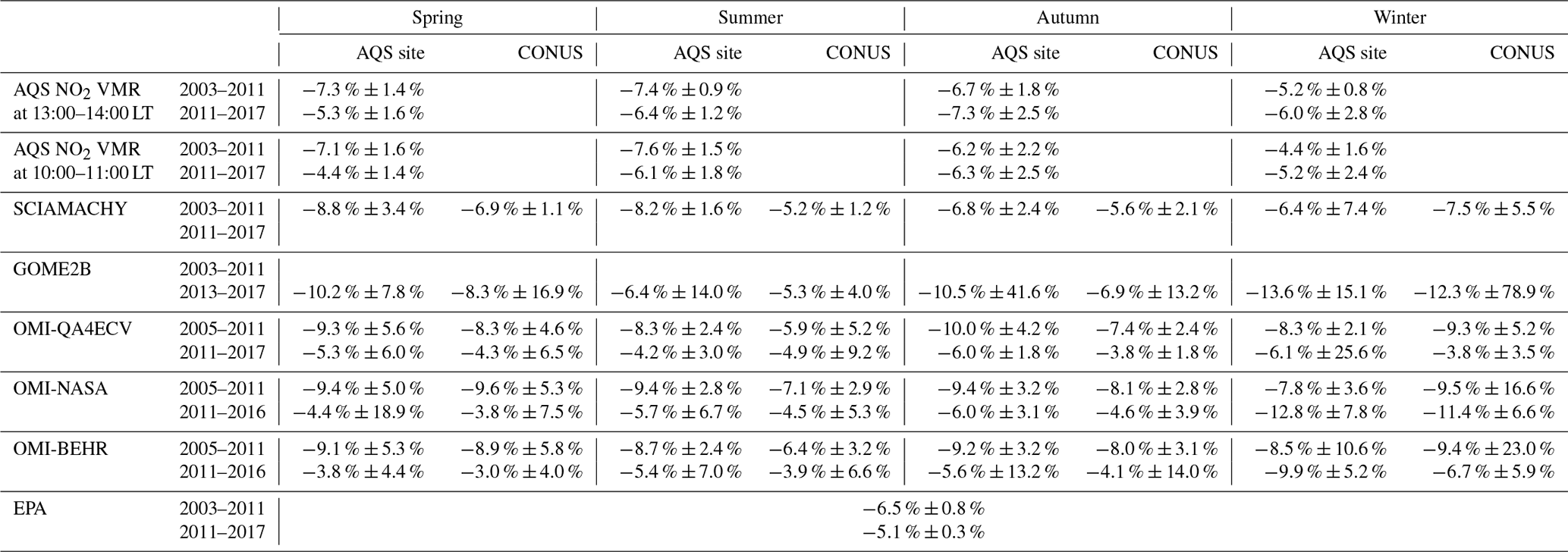
The US anthropogenic NOx emissions during the 2010s declined dramatically compared to the mid-2000s (EPA, 2018b; Xing et al., 2013) due to stricter air quality regulations and emission control technology improvements, such as the phase-in of Tier II vehicles during 2004–2009 and the switch of power plants from coal to natural gas (De Gouw et al., 2014; McDonald et al., 2018). The overall reduction (about 30 %–50 %) of anthropogenic NOx emissions from the mid-2000s to the 2010s was corroborated by observed decreases in vehicle NOx emission factors, NO2 surface concentrations, nitrate wet deposition flux (Fig. S1 in the Supplement), and NO2 tropospheric vertical column densities (TVCDs) (Bishop and Stedman, 2015; Georgoulias et al., 2019; Li et al., 2018; McDonald et al., 2018; Miyazaki et al., 2017; Russell et al., 2012; Tong et al., 2015). However, the detailed NOx emission changes after the Great Recession (from December 2007 to June 2009) are highly uncertain. On the one hand, the U.S. Environmental Protection Agency (EPA) estimated that the Great Recession had a slight impact on the anthropogenic NOx emission trend and the anthropogenic NOx emissions decreased steadily from 2002 to 2017 (Fig. S2), although the emission decrease rate slowed down by about 20 % after 2010 (−5.8 % yr−1 for 2002–2010 and −4.7 % yr−1 for 2010–2017; Table 1) (EPA, 2018b). Fuel-based emission estimates in Los Angeles also showed a steady decrease in anthropogenic NOx emissions after 2000 and a small impact of the Great Recession on the anthropogenic NOx emission decrease trend (Hassler et al., 2016). The continuous decrease in anthropogenic NOx emissions was consistent with the ongoing reduction in vehicle emissions (McDonald et al., 2018). On the other hand, Miyazaki et al. (2017) and Jiang et al. (2018) found that the US NOx emissions derived from satellite NO2 TVCDs, including OMI (the Ozone Monitoring Instrument), SCIAMACHY (SCanning Imaging Absorption SpectroMeter for Atmospheric CHartography), and GOME-2A (Global Ozone Monitoring Experiment 2 onboard METOP-A), were almost flat from 2010–2015 and suggested that the decrease in NOx emissions was only significant before 2010, which was completely different from the bottom–up and fuel-based emission estimates.
Table 1Summary of trends of satellite NO2 TVCD products, NO2 surface measurements, and EPA anthropogenic NOx emissions from different studies.
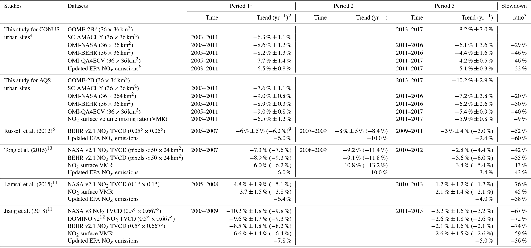
1 Since different studies used different time division methods, we list
the period of each study in the table.
2 Trends are based on an exponential model: , where “y” denotes year and “y0” denotes the initial year, “E(y)” denotes the value at year “y” and “E0” denotes the value at the initial year, and r−1 is the relative trend.
3 Slowdown ratios = trend in “period 3”∕trend in “period 1”−1.
4 Trends in our study are calculated based on the national seasonal
trends shown in Table 3.
5 The information on satellite products used in this study is
summarized in Table S2.
6 We updated EPA anthropogenic NOx emissions with the newest
Continuous Emission Monitoring Systems (CEMS) datasets. Figure S2 shows the
comparison between our updated and original EPA anthropogenic NOx
emissions (EPA, 2018b).
7 Denotes the averaged trends of 13:00 and 10:00 local time (LT) based on the values
in Table 3.
8 The study used NO2 TVCD from urban and power plant grid cells
across the US.
9 Since previous studies used linear models to calculate trends and the
results are sensitive to their calculation methods and the selection of
initial years, we recalculate the trends based on the above exponential
model, which makes all the results consistent. Our results are the bold
numbers in parentheses, while the numbers in normal font are from
the original publications.
10 The study uses NO2 TVCD and surface concentrations from Los
Angeles, Dallas, Houston, Atlanta, Philadelphia, Washington, D.C., New York,
and Boston.
11 The two studies used the EPA Air Quality System (AQS) NO2
surface measurements and coincident satellite NO2 TVCD data over the US.
12 DOMINO: Dutch OMI NO2 products.
A complicating factor in inferring anthropogenic NOx emission trends from the observations of NO2 surface concentrations and satellite NO2 TVCDs is their nonlinear dependences on anthropogenic NOx emissions (Gu et al., 2013, 2016; Lamsal et al., 2011). Although the decrease rates of both NO2 surface concentrations and coincident OMI NO2 TVCDs slowed down after the Great Recession over the United States, Tong et al. (2015), Lamsal et al. (2015), and Jiang et al. (2018) found that the slowdown of the decrease rates derived from NO2 surface concentrations is 12 %–79 % less than those of NO2 TVCDs (Table 1). Secondly, the slowdown of the decrease rates of NO2 surface concentrations and OMI TVCDs over cities and power plants (Russell et al., 2012; Tong et al., 2015) is significantly less than those over the whole contiguous United States (CONUS) (Jiang et al., 2018; Lamsal et al., 2015). Moreover, Zhang et al. (2018) found that filtering out lightning-affected measurements could significantly improve the comparison of NO2 surface concentration and OMI NO2 TVCD trends over the CONUS.
In this study, we carefully investigate the relationships among anthropogenic NOx emissions, NO2 surface concentrations, and NO2 TVCDs over the CONUS and evaluate the impact of the relationships on inferring anthropogenic NOx emission changes and trends from surface and satellite observations. Section 2 describes the model and datasets used in this study, including the Regional chEmistry and trAnsport Model (REAM), the EPA Air Quality System (AQS) NO2 surface observations, and NO2 TVCD products from OMI, GOME-2A, GOME-2B (GOME2 onboard METOP-B), and SCIAMACHY. In Sect. 3, we examine the nonlinear relationships among anthropogenic NOx emissions, NO2 surface concentrations, and NO2 TVCDs using model simulations. Accounting for the effects of background sources, physical processes, and chemical nonlinearity, we then investigate the anthropogenic NOx emission trends and changes from 2003 to 2017 over the CONUS. Finally, Sect. 4 gives a summary of the study.
2.1 REAM
REAM has been applied and evaluated in many research applications including ozone simulation and forecast, emission inversion and evaluations, and mechanistic studies of chemical and physical processes (Alkuwari et al., 2013; Cheng et al., 2017, 2018; Choi et al., 2008a, b; Gu et al., 2013, 2014; Koo et al., 2012; Liu et al., 2012, 2014; Wang et al., 2007; Yang et al., 2011; Zhang et al., 2017, 2018; Zhang and Wang, 2016; Zhao and Wang, 2009; Zhao et al., 2009a, 2010). REAM as used in this work, the model domain of which is shown in Fig. 3, has 30 vertical layers in the troposphere, and the horizontal resolution is 36×36 km2. The model is driven by meteorology fields from a Weather and Research Forecasting (WRF, version 3.6) model simulation initialized and constrained by the NCEP coupled forecast system model version 2 (CFSv2) products (Saha et al., 2011). The chemistry mechanism is based on GEOS-Chem v11.01 with updated reaction rates and aerosol uptake of isoprene nitrates (Fisher et al., 2016). Chemistry boundary conditions and initializations are from a GEOS-Chem (2∘ × 2.5∘) simulation. Hourly anthropogenic emissions on weekdays are based on the 2011 National Emission Inventory (NEI2011), while weekend anthropogenic emissions are set to be two-thirds of the weekday emissions (Beirle et al., 2003; Choi et al., 2012). Biogenic volatile organic compound (VOC) emissions are estimated using the Model of Emissions of Gases and Aerosols from Nature (MEGAN) v2.10 (Guenther et al., 2012). NOx emissions from soils are based on the Yienger and Levy (YL) scheme (Li et al., 2019; Yienger and Levy, 1995). The cloud-to-ground (CG) lightning flashes are calculated following Choi et al. (2005) and Zhao et al. (2009a) with the parameterization of the CG flash rate as a function of convective mass fluxes and convective available potential energy (CAPE). The ratios of intra-cloud (IC) lightning flashes to CG flashes are parameterized as a function of the height between the freezing layer and the cloud top (Luo et al., 2017; Price and Rind, 1992). In this study, 250 mol of NO are emitted per CG or IC flash (Zhao et al., 2009a). As a result, on weekdays in July 2011, REAM has mean anthropogenic NOx emissions of 7.4×10¹⁰ molecules cm−2 s−1, mean soil NOx emissions of 1.2×10¹⁰ molecules cm−2 s−1, and mean lightning NOx emissions of 3.4×10¹⁰ molecules cm−2 s−1 over the CONUS.
2.2 Satellite NO2 TVCDs
In this study, we use NO2 TVCD products from four satellite sensors in the past decade, including SCIAMACHY, GOME-2A, GOME-2B, and OMI – the spectrometers onboard sun-synchronous satellites to monitor atmospheric trace gases. The SCIAMACHY instrument onboard the Environmental Satellite (ENVISAT) has an Equator overpass time of 10:00 local time (LT) and a nadir pixel resolution of 60×30 km2. The GOME-2 instruments on Metop-A (named GOME-2A) and Metop-B (GOME-2B) satellites cross the Equator at 09:30 LT and have a nadir resolution of 80×40 km2. After 15 July 2013, the nadir resolution of GOME-2A became 40×40 km2 with a smaller scanning swath. The OMI onboard the EOS-Aura satellite has a nadir resolution of 24×13 km2 and overpasses the Equator around 13:45 LT. More detailed information about these instruments is summarized in Table S1. These instruments measure backscattered solar radiation from the atmosphere in the ultraviolet and visible wavelength. The radiation measurements in the wavelength of 402–465 nm are then used to retrieve NO2 vertical column densities (VCDs). The retrieval process consists of three steps: (1) converting radiation observations to NO2 slant column densities (SCDs) by using the differential optical absorption spectroscopy (DOAS) spectral fitting method; (2) separating tropospheric SCDs and stratospheric SCDs from the total NO2 SCDs; (3) dividing the NO2 tropospheric SCDs by the tropospheric air mass factors (AMFs) to compute TVCDs.
The product archives we use in this study include GOME-2B (TM4NO2A v2.3), SCIAMACHY (QA4ECV v1.1), GOME-2A (QA4ECV v1.1), OMI (QA4ECV v1.1, hereafter referred to as OMI-QA4ECV), OMNO2 (SPv3, hereafter referred to as OMI-NASA), and the Berkeley High-Resolution NO2 products (v3.0B, hereafter referred to as OMI-BEHR). OMI-BEHR uses the tropospheric SCDs from OMI-NASA products but updates some inputs for the tropospheric AMF calculation (Laughner et al., 2018b). These product archives have been previously validated (Boersma et al., 2018; Drosoglou et al., 2017, 2018; Krotkov et al., 2017; Laughner et al., 2018b; Wang et al., 2017; Zara et al., 2018). Generally, the pixel-size uncertainties of these products are >30 % over polluted regions under clear-sky conditions. We summarize the basic information about these products in Table S2. To keep the high quality and sampling consistency of NO2 TVCD datasets, we chose pixel-size NO2 TVCD data using the criteria listed in Table S3. After the selection, we re-gridded the pixel-size data into the REAM 36×36 km2 grid cells and calculated the seasonal means of each grid cell with corresponding daily values on weekdays (winter: January, February, and December; spring: March, April, and May; summer: June, July, and August; autumn: September, October, and November). We excluded weekend data in this study to minimize the impacts of weekend NOx emission reduction, leading to different NO2 TVCDs between weekdays and weekends (Fig. S3).
Satellite TVCD measurements can show large variations and apparent discontinuities due in part to the effects of cloud, lightning NOx, the shift in satellite pixel coverage, and retrieval uncertainties (Fig. S3; e.g., Boersma et al., 2018; Zhang et al., 2018). However, continuous and consistent measurements are required for reliable trend analyses. In addition to the criteria of data selection in Table S3, we compute the seasonal relative 90th percentile confidence interval, defined as RCI = (X(95th percentile) – X(5th percentile)) / mean(X), where X is the daily NO2 TVCD for a given season. To compute the seasonal trend, we require that RCI is <50 % for the selected season every year in the analysis period (Table S3). About 45 % of data are removed as a result.
2.3 Surface NO2 measurements
Hourly surface NO2 measurements from 2003 to 2017 are from the EPA AQS monitoring network (archived on https://www.epa.gov/outdoor-air-quality-data, last access: 27 June 2018). Most AQS monitoring sites use the Federal Reference Method (FRM) gas-phase chemiluminescence to measure NO2. Few sites use the Federal Equivalent Method (FEM) photolytic chemiluminescence or the cavity attenuated phase shift spectroscopy (CAPS) method. FRM and FEM are indirect methods, in which NO2 is first converted to NO and then NO is measured through chemiluminescence measurement of NO2* produced by NO + O3. The difference is that FRM uses heated catalysts for the conversion of NO2 to NO and FEM uses photolysis of NO2 to NO. The conversion to NO in the FRM instruments is not specific to NO2, and non-NOx active nitrogen compounds (NOz) can also be reduced by the catalysts, which would cause high biases of NO2 measurements, while the FEM is sensitive to the photolysis conversion efficiency of NO2 to NO (Beaver et al., 2012, 2013; Lamsal et al., 2015). The CAPS method directly determines NO2 concentrations based on an NO2-induced phase shift measured by a photodetector. The CAPS instrument operates at a wavelength of about 450 nm and may overestimate NO2 concentrations due to the absorption of other molecules at the same wavelength (Beaver et al., 2012, 2013; Kebabian et al., 2005).
Due to the different characteristics of the above three methods and demonstrated biases between the FRM and the FEM by Lamsal et al. (2015), we firstly investigate the measurement discrepancies among the above three methods. There are three sites having FRM and FEM measurements simultaneously during some periods from 2013 to 2014, two sites having both FRM and CAPS data during some periods from 2015 to 2016, and one site using all three measurement methods during some periods in 2015. Figure S4 shows the hourly averaged ratios of FEM and CAPS to FRM data for four seasons during 2013–2016. The CAPS∕FRM ratios are in the range of 0.94–1.06, and the FEM∕FRM ratios are 0.86–1.11. Furthermore, Zhang et al. (2018) discussed that the relative trends are not affected by scaling the observation data. As in the work by Zhang et al. (2018), we analyze the relative trends in the surface NO2 data. We, therefore, did not scale the FRM data. At sites with FEM or CAPS measurements, we use these measurements in place of FRM data. If both FEM and CAPS data are available, we use the averages of the two datasets.
Since NO2 surface concentrations have significant diurnal variations (Fig. S5), we choose the data at 09:00–10:00 LT for comparison with GOME-2A/2B data, those at 10:00–11:00 LT for comparison with SCIAMACHY data, and those at 13:00–14:00 LT for OMI data. The seasonal RCI < 50 % requirement is also used here to be consistent with the analysis of satellite TVCD data, and thus about 1.5 % of the data is removed. We also require that the measurement site must have valid measurements in the aforementioned 3 h for at least one season from 2003 to 2017. The locations of the 179 selected sites using the site selection criteria are shown in Fig. 1. The region definitions follow the U.S. Census Bureau (https://www2.census.gov/geo/pdfs/maps-data/maps/reference/us_regdiv.pdf, last access: 6 February 2019).
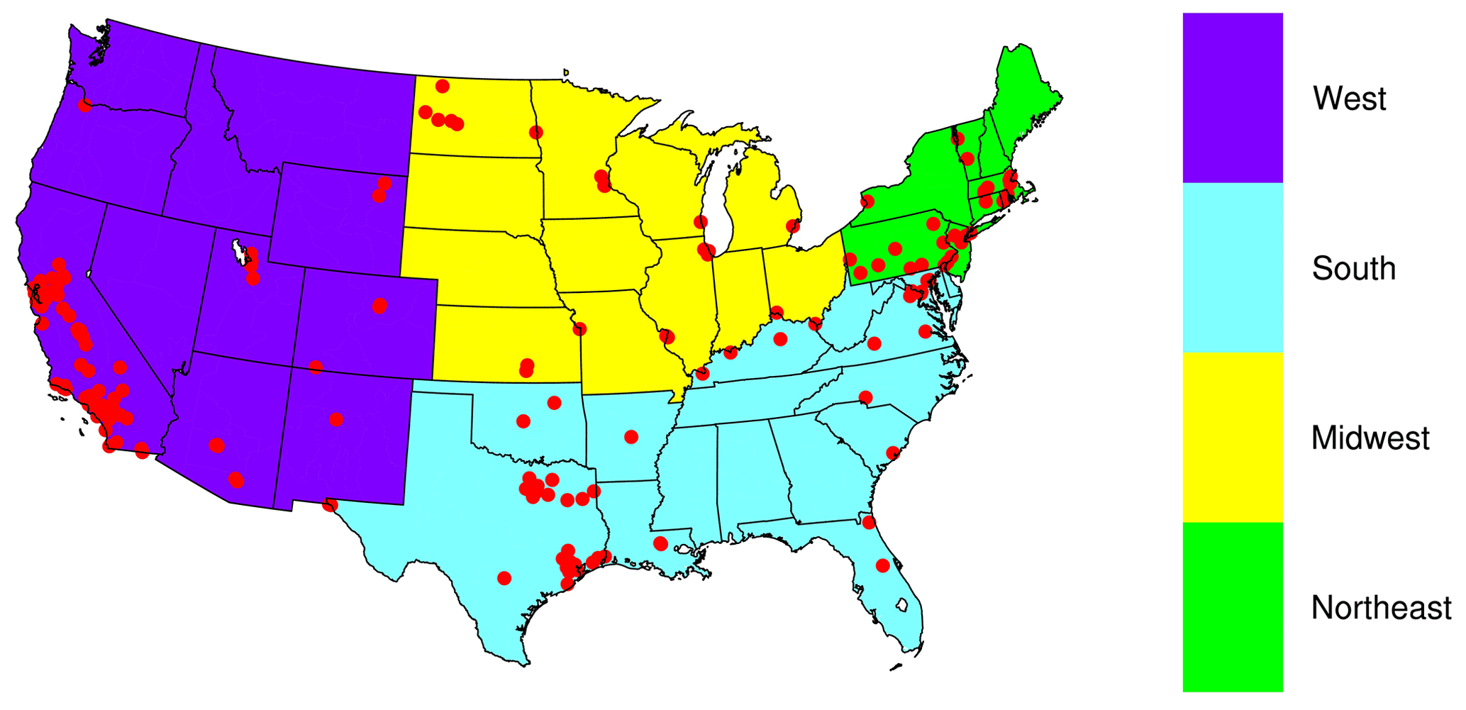
Figure 1Region definitions and locations of NO2 surface observation sites used in this study.
3.1 Nonlinear relationships among anthropogenic NOx emissions, NO2 surface concentrations, and NO2 TVCDs
NO2 surface concentrations and NO2 TVCDs are not linearly correlated with NOx emissions due to chemical nonlinearity, NO2 hydrolysis on aerosols (NO2 , dry deposition, transport effects, and background sources (Gu et al., 2013; Lamsal et al., 2011). Therefore, it is necessary to first investigate the nonlinearities among NOx emissions, NO2 surface concentrations, and TVCDs over the CONUS before we compare the trends between NO2 surface concentrations and TVCDs. The nonlinearity between NOx emission and NO2 TVCD is analyzed by examining the local sensitivity of NO2 TVCD to NOx emissions (Gu et al., 2013; Lamsal et al., 2011; Tong et al., 2015), which is defined as β in Eq. (1). We further define γ as the sensitivity of NO2 surface concentration to NOx emission:
where E denotes NOx emission and E denotes the change in NOx emission; Ω denotes NO2 TVCD, c denotes surface NO2 concentration, and ΔΩ and Δc denote the corresponding changes.
We computed β and γ values for July 2011 over the CONUS using REAM. To compute local β and γ values, we added another independent group of chemistry species (“group 2”) in REAM in order to compute the standard and sensitivity simulations concurrently. The original chemical species in the model (“group 1”) were used in the standard simulation. For group 2 chemical species, anthropogenic NOx emissions were reduced by 15 %. In the model simulation, we first computed the advection of group 1 tracers. The horizontal tracer fluxes were therefore available. All influxes into a grid cell for the group 2 tracer simulation were from the group 1 tracer simulation; only outfluxes were computed using group 2 tracers. The outflux was one way in that nitrogen species were transported out but the transport did not affect adjacent grid cells because the influxes were from the group 1 tracer simulation. Using this procedure, the effects of anthropogenic NOx emission reduction were localized. The β and γ values were computed by the ratio of TVCD and surface concentration changes to a 15 % change in anthropogenic NOx emissions.
Figure 2 shows the distributions of our β and γ ratios as a function of anthropogenic NOx emissions for July 2011 over the CONUS. Results essentially the same as Fig. 2 were obtained when a perturbation of 10 % was used for anthropogenic NOx emissions. Figure S6 shows the distributions of NO2 TVCD fraction in the boundary layer at 13:00–14:00 LT and 10:00–11:00 LT and the fraction of soil NOx emissions in all surface sources (soil + anthropogenic) on weekdays for July 2011. In Fig. S7, we analyzed the contributions of background sources, chemical nonlinearity, and other factors (transport, NO2 hydrolysis on aerosols, and dry deposition) to the nonlinear relationships (β and γ) among anthropogenic NOx emissions, NO2 surface concentrations, and NO2 TVCDs. While the model simulation is for 1 summer month, several key points on the surface and column concentration sensitivities to anthropogenic NOx emissions have implications for comparing the trends of AQS and satellite TVCD data.
-
Both β and γ values are negatively correlated with anthropogenic NOx emissions due to chemical nonlinearity, transport, and background NOx contributions (Figs. 2, S6, and S7) (Gu et al., 2016; Lamsal et al., 2011). It is consistent with the distribution of β as a function of NOx emissions in China (Gu et al., 2013), although the β ratios for the US are generally larger than for China due primarily to different emission distributions of NOx and VOCs and regional circulation patterns (Zhao et al., 2009b).
-
The uncertainties of β and γ values increase significantly as anthropogenic NOx emissions decrease, which means regions with low anthropogenic NOx emissions are more sensitive to environmental conditions, such as NOx transport from nearby regions which may even produce negative β and γ values (Figs. 2 and S7).
-
The value of γ is generally less than β, especially for low anthropogenic NOx emission regions, which reflects the significant contribution of free tropospheric NO2 to NO2 TVCD but not to NO2 surface concentrations (Figs. 2, S6, and S7).
-
Generally, the standard deviations of β and γ tend to be larger at 10:00–11:00 LT than at 13:00–14:00 LT, reflecting a stronger transport effect due to weaker chemical losses in the morning (Figs. 2 and S7).
-
Both β and γ values are significantly less than 1 at 13:00–14:00 LT (β=0.75 and γ=0.84) when anthropogenic NOx emissions are molecules cm−2 s−1, but they are close to 1 at 10:00–11:00 LT (β=0.97 and γ=1.03), which reflects stronger chemistry nonlinearity at noontime than in the morning (Figs. 2 and S7).
-
Both background sources and non-emission factors contribute much more to β and γ values in low anthropogenic NOx emission regions than in high anthropogenic NOx emission regions (Fig. S7).
-
Chemical nonlinearity contributes much less to β and γ values than background sources and transport effects in low anthropogenic NOx emission regions (Fig. S7).
-
Generally, non-emission factors (mainly transport) contribute more to β and γ values than background sources in low anthropogenic NOx emission regions (Fig. S7c and d) except for the first bin where background sources contribute more to β and γ values than non-emission factors at 10:00–11:00 LT, which is partly caused by some grid cells with extremely low anthropogenic NOx emissions, increasing the mean contributions of background sources in the first bin.

Figure 2Distributions of β (a) and γ (b) ratios as a function of anthropogenic NOx emissions on weekdays for July 2011 over the CONUS. “13:00–14:00 LT” is for OMI, and “10:00–11:00 LT” is for SCIAMACHY and GOME-2A/2B. The data are binned into nine groups based on anthropogenic NOx emissions: E∈ (0, 21), [21, 22), [22, 23), [23, 24), [24, 25), [25, 26), [26, 27), [27, 28), [28, 29) × 1010 molecules cm−2 s−1. Here, (0, 21) denotes 0< emissions <21, and [21, 22) denotes 21≤ emissions <22, similar to other intervals. The green dashed line denotes a value of 1. Error bars denote standard deviations.
The largely varying β and γ values for anthropogenic NOx emissions <1011 molecules cm−2 s−1 imply that the trends derived from satellite TVCD data do not directly represent anthropogenic NOx emissions and that the variations in TVCD data may not be comparable to the corresponding surface NO2 concentrations. We define a region a “urban” if anthropogenic NOx emissions from NEI2011 are >1011 molecules cm−2 s−1. All the other regions are defined as “rural”. Figure 3 shows the distributions of anthropogenic NOx emissions and urban and rural regions defined in this study. Such defined urban regions account for 69.8 % of the total anthropogenic NOx emissions over the CONUS, the trend of which is, therefore, representative of anthropogenic emission changes. A caveat is that some urban regions would become rural if anthropogenic NOx emissions decreased after 2011 as the EPA anthropogenic NOx emission trend suggested (Fig. S2). In a sensitivity study, we define an urban region using a stricter criterion of anthropogenic NOx emissions molecules cm−2 s−1, and the analysis results are similar to those shown in the next section.
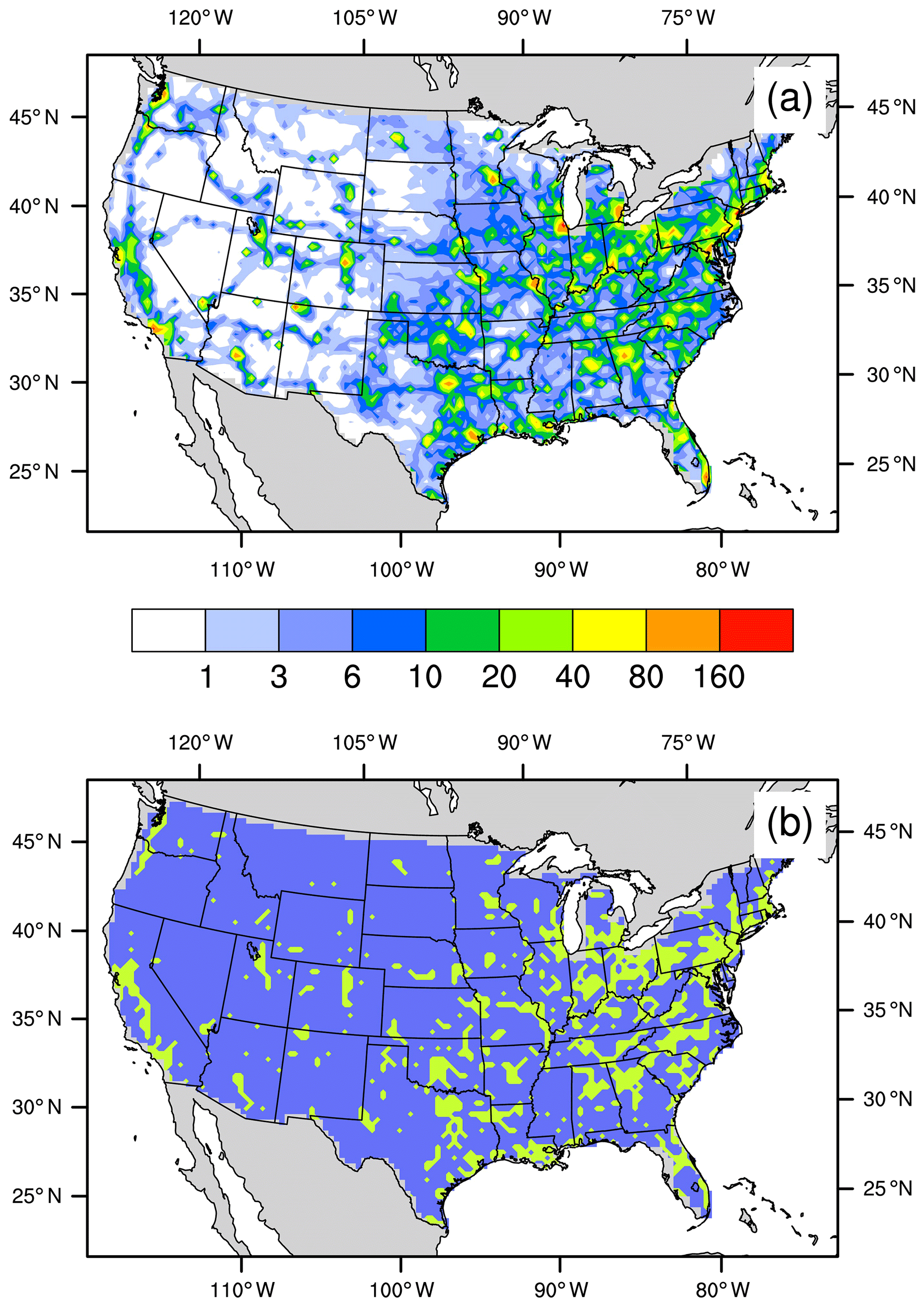
Figure 3Spatial distributions of (a) anthropogenic NOx emissions (unit: 1010 molecules cm−2 s−1) and (b) urban regions satisfying our selection criteria. In (b), light green and blue denote the resulting urban and rural regions, respectively.
3.2 Trend comparisons between NO2 AQS surface concentrations and coincident satellite NO2 tropospheric VCD over urban and rural regions
By using anthropogenic NOx emissions of 1011 molecules cm−2 s−1 as the threshold value, 157 AQS sites are urban, and the remaining 22 sites are rural. Their properties are summarized in Table 2. Figure 4 shows the relative annual variations in AQS NO2 surface measurements at 13:00–14:00 LT and coincident OMI-QA4ECV NO2 TVCD data from 2005 to 2017 in each season for urban and rural regions. The contrast between the two regions is apparent in all seasons. For comparison purposes, we scale the time series of TVCD and AQS surface NO2 to their corresponding 2005 values, and the resulting data are therefore unitless. Over urban regions, NO2 surface concentrations are highly correlated with NO2 TVCDs (TVCD = 1.03 × AQS + 0.11, R2=0.98), reflecting the comparable and stable β and γ values (Fig. 2). However, over rural regions, the scaled TVCD data significantly deviate from AQS NO2 data (TVCD = 1.15 × AQS + 0.09, R2=0.87). It is noteworthy that the discrepancies between urban and rural data are smaller in winter than in spring, summer, and autumn due to a more dominant role of transport than chemistry and lower natural NOx emissions in winter.
Table 2Properties of urban and rural regions in July 2011.
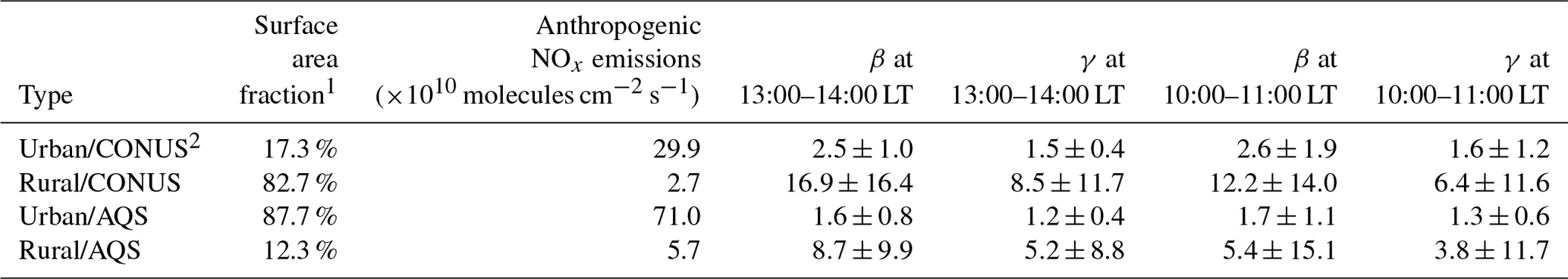
1 “Fraction” denotes the percentages of urban or rural data points for the whole CONUS or all AQS sites. 2 “Urban-CONUS” denotes CONUS urban grid cells; “Urban-AQS” denotes AQS urban site grid cells.
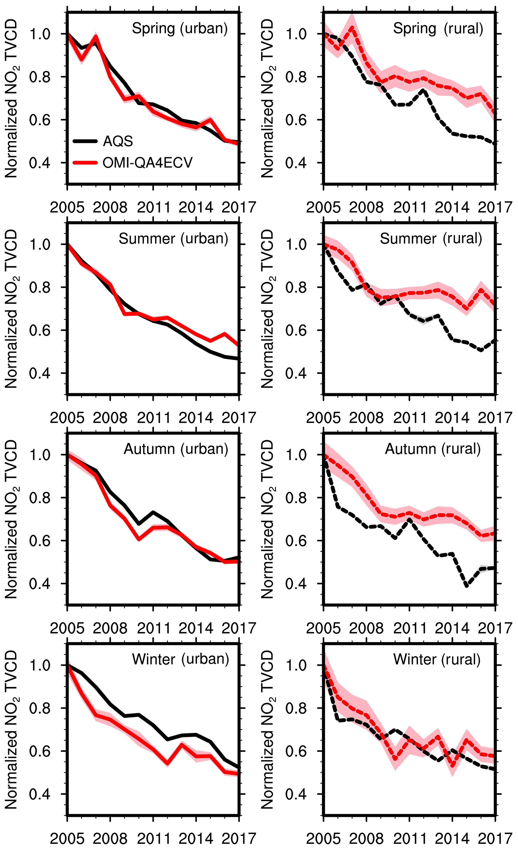
Figure 4Relative annual variations in AQS NO2 surface concentrations and coincident OMI-QA4ECV NO2 TVCD in each season from 2005 to 2017 for urban (left column) and rural (right column) regions. The observation data are scaled by the corresponding 2005 values. Black and red lines denote AQS surface observations and OMI-QA4ECV NO2 TVCDs, respectively. Shading in a lighter color is added to show the standard deviation of the results; when uncertainty is small due in part to a large number of data points, shading may not show up.
We also examine the correlations of AQS NO2 surface concentrations with coincident OMI-NASA, OMI-BEHR, SCIAMACHY, GOME-2A, and GOME-2B TVCD measurements. The results of OMI-NASA and OMI-BEHR are similar to those of OMI-QA4ECV (Fig. 4). SCIAMACHY and GOME-2B TVCD observations at 09:00–11:00 LT also show a large contrast between urban (SCIAMACHY: TVCD = 0.92 × AQS − 0.005, R2=0.94; GOME-2B: TVCD = 0.54 × AQS + 0.56, R2=0.96) and rural regions (SCIAMACHY: TVCD = 0.77 × AQS + 0.83, R2=0.63; GOME-2B: TVCD = 0.46 × AQS + 0.73, R2=0.59). The correlation of coincident GOME-2A NO2 TVCD data with AQS surface concentrations is poor for rural (TVCD = 0.65 × AQS + 0.56, R2=0.44) and urban (TVCD = 0.31 × AQS + 0.56, R2=0.21) regions (Fig. S8), which likely reflects the degradation of the GOME-2A instrument causing a significant increase in NO2 SCD uncertainties (Boersma et al., 2018). Therefore, we excluded GOME-2A in the analysis hereafter.
We further investigate OMI-QA4ECV NO2 TVCD relative annual variations from 2005 to 2017 over the regions with different anthropogenic NOx emissions in Fig. 5. We find clear flattening of NO2 TVCD variations as anthropogenic NOx emissions decrease, which is consistent with the above analysis. Similar to Fig. 4, the spread of TVCD variation is much less in winter than the other seasons. The differences between Figs. 5 and 4 are due to a much larger dataset used in the former than the latter. Only coincident AQS and OMI-QA4ECV data are used in Fig. 4, but all OMI-QA4ECV data are used in Fig. 5.
3.3 Trend analysis of AQS NO2 surface concentrations, satellite TVCDs, and updated EPA NOx emissions
We first updated the Continuous Emission Monitoring Systems (CEMS) measurement data used in the EPA NOx emission trend datasets with the newest datasets obtained from https://ampd.epa.gov/ampd/ (last access: 17 June 2018). As shown in Fig. S2, the updated CEMS data lead to a reduction in anthropogenic NOx emissions during the Great Recession (2008–2009) and a recovery period in 2010–2011. The sharp drop during the Great Recession and the flattening trend right after the Great Recession are captured by OMI NO2 and SCIAMACHY TVCD products (Figs. 4, 6, and S9) and AQS NO2 surface measurements (Figs. 4, 6, and S5) and are also noted by Russell et al. (2012) and Tong et al. (2015) (Table 1).
In Fig. 6, we show the comparisons among the relative variations in the updated EPA anthropogenic NOx emissions, AQS NO2 surface measurements at 10:00–11:00 LT and 13:00–14:00 LT, and coincident satellite NO2 TVCDs for urban regions in four seasons from 2003 to 2017. Also shown are the comparisons among the updated EPA anthropogenic NOx emissions and satellite NO2 TVCDs. There are many more data points for the latter comparison because the data selection is no longer limited to those coincident with the AQS surface data, and therefore, the uncertainty spread is much lower. The comparisons, in general, show that the updated EPA anthropogenic NOx emissions, AQS surface measurements, and satellite TVCD data are in agreement. The agreement of decreasing trends among the datasets is just as good for the post-2011 period as the pre-2011 period. This result differs from Miyazaki et al. (2017) and Jiang et al. (2018), who suggested no significant decreasing trend for OMI TVCD data and inversed NOx emissions after 2010. The disagreement can be explained by the results of Fig. 5. Including the low anthropogenic NOx emission regions leads to underestimates of NOx decreases. Since the area of low anthropogenic NOx emission regions is larger than high anthropogenic NOx emission regions (Table 2), the arithmetic averaging will lead to a large weighting of rural observations, which do not reflect anthropogenic NOx emission changes. Miyazaki et al. (2017) and Jiang et al. (2018) included all regions in their analyses, but we exclude rural regions. Figure S9 shows the seasonal variations if the TVCDs over rural regions are included; the result shows a much lower decreasing rate of TVCDs over the CONUS. The much slower satellite TVCD trends for regions with low NOx emissions was previously discussed by Zhang et al. (2018). In addition, Miyazaki et al. (2017) and Jiang et al. (2018) conducted NOx emission inversions by using the Model for Interdisciplinary Research on Climate (MIROC)-Chem with a coarse resolution of 2.8∘ × 2.8∘, which was insufficient to separate urban and rural regions and might distort predicted NO2 TVCDs and inversed NOx emissions due to nonlinear effects (Valin et al., 2011; Yu et al., 2016), which is another possible reason for their finding of flattening NOx emission trends after 2010.
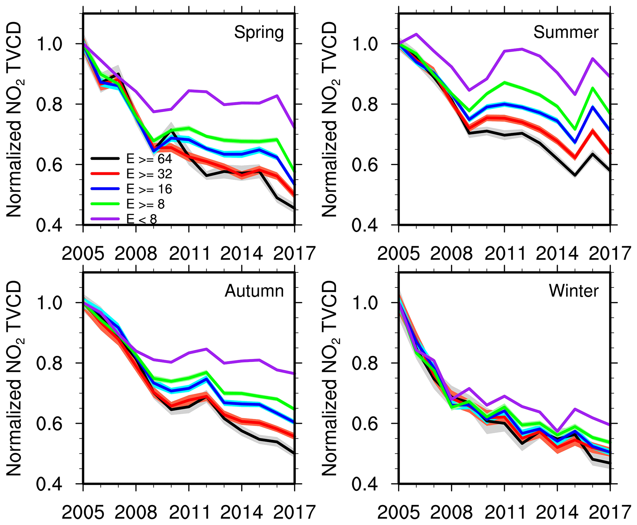
Figure 5Relative annual variations in OMI-QA4ECV NO2 TVCD for different anthropogenic NOx emission groups based on NEI2011 in each season from 2005 to 2017. “” denotes grid cells with anthropogenic NOx emissions over 64×1010 molecules cm−2 s−1. “” denotes grid cells with anthropogenic NOx emissions equal to or larger than 32×1010 molecules cm−2 s−1 but less than 64×1010 molecules cm−2 s−1. “” and “” have similar meanings as “”. “E<8” denotes grid cells with anthropogenic NOx emissions less than 8×10¹⁰ molecules cm−2 s−1. Shading in a lighter color is added to show the standard deviation of the results; when uncertainty is small due in part to a large number of data points, shading may not show up.
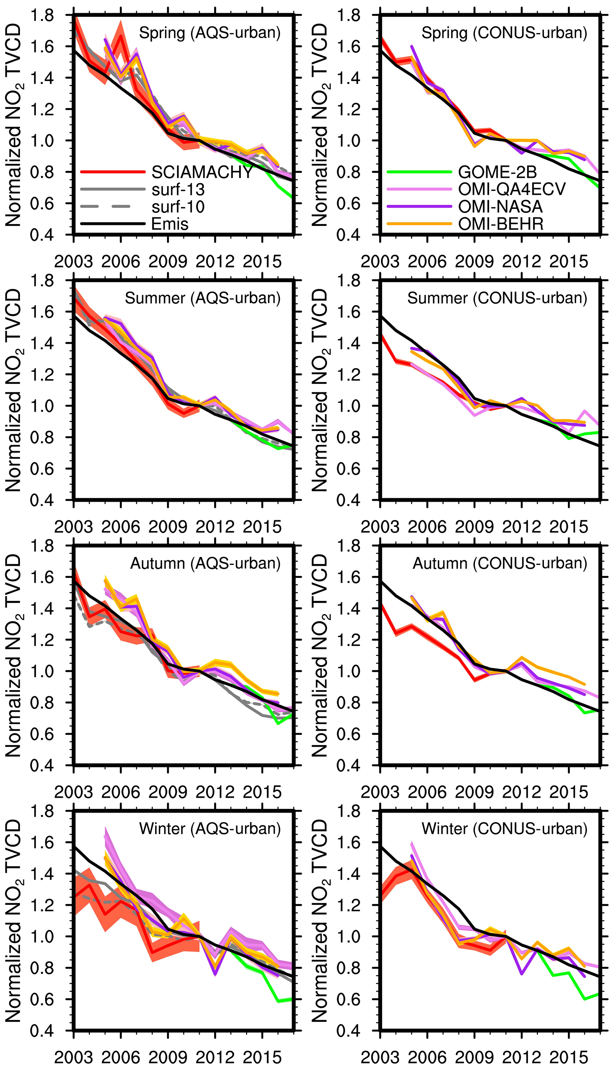
Figure 6Relative variations in AQS NO2 surface measurements at 13:00–14:00 LT and 10:00–11:00 LT, updated EPA anthropogenic NOx emissions, and satellite NO2 TVCD data over the AQS urban sites (left column) and the CONUS urban regions (right column) for four seasons. AQS NO2 surface measurements are not included in the right column. All datasets are scaled by their corresponding values in 2011 except for GOME-2B. For GOME-2B, we firstly normalized the values in each season to the corresponding 2013 values and plotted the relative changes from the 2013 EPA point of each season to make the GOME-2B relative variations comparable to the other datasets. Shading in a lighter color is added to show the standard deviation of the results; when uncertainty is small due in part to a large number of data points, shading may not show up.
We summarize the decreasing rates of NO2 after the Great Recession in Table 3. To minimize the effect of the sharp decrease and the subsequent recovery, we chose to analyze the post-2011 period. Table 3 summarizes the results for each season, while Table 1 gives the averaged annual decreasing trends. Generally, Tables 1 and 3 confirm the continuous decreases in AQS surface observations, satellite NO2 TVCD, and updated EPA anthropogenic NOx emissions after 2011 as in Fig. 6, but the decreasing rates are lower than the pre-2011 period. Over the AQS urban sites, the slowdown magnitudes are 9 % for AQS surface observations and 20 %–40 % for satellite NO2 TVCD measurements, which may reflect in part smaller γ than β values (Table 2). Our estimated slowdown magnitudes are significantly lower than Lamsal et al. (2015) and Jiang et al. (2018) (Table 1), which might be caused by their different data processing methods, such as including AQS sites with incomplete measurement records (Silvern et al., 2019).
Table 3Summary of national trends of updated EPA anthropogenic NOx emissions, AQS NO2 surface concentrations at 13:00–14:00 LT and 10:00–11:00 LT, and satellite NO2 TVCD products for four seasons during different periods.∗
∗ We calculate trends by using the exponential model described in Table 1.
Over the CONUS urban regions, updated EPA anthropogenic NOx emissions show a slowdown of 22 % compared to 29 %–46 % for three OMI NO2 TVCD products. The difference is partially due to the β ratio of 2.5±1.0 at 13:00–14:00 LT over the CONUS urban regions (Table 2). Satellite NO2 TVCD measurement uncertainties also contribute to the difference. From 2013 to 2017, GOME-2B NO2 TVCDs decrease more than OMI products, especially in spring, autumn, and winter (Tables 1 and 3). Finally, trend analyses in different regions (Fig. 7 and Table S4) indicate that generally, the Midwest has the least slowdown of the decreasing rate for urban OMI NO2 TVCD (−14 % on average) after 2011 compared to the Northeast (−30 %), South (−34 %), and West (−28 %).
The results presented in this study are qualitatively in agreement with the work by Silvern et al. (2019). The two studies were independent. Therefore, the foci of the studies are different despite reaching similar conclusions. While we focused on understanding the detailed data analysis of Jiang et al. (2018) and limited the use of model simulation results so that our results can be compared to the previous study directly, Silvern et al. (2019) relied more on multiyear model simulations. As a result, Silvern et al. (2019) can clearly identify the contributions of the NO2 columns by natural emissions and make use of additional observations such as nitrate deposition fluxes. They also identified model biases in simulating the trends of NO2 TVCDs by missing natural emissions in the free troposphere. Our study, on the other hand, explored the data analysis procedure through which the trend of anthropogenic emissions can be derived from satellite observations and its limitations.
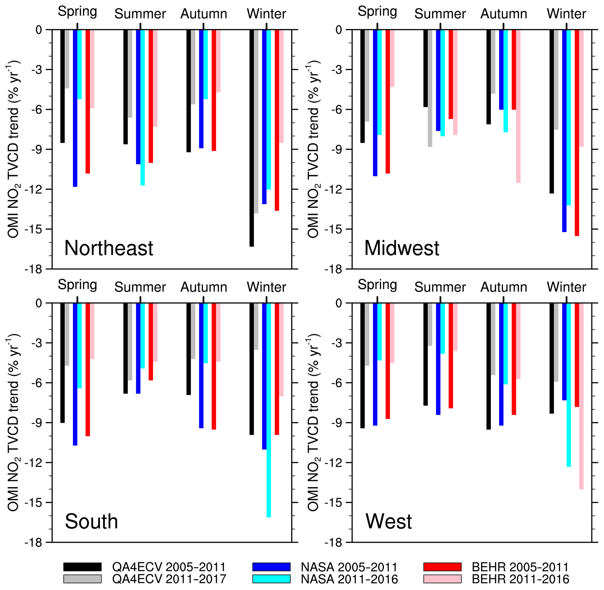
Figure 7Pre- and post-2011 OMI NO2 TVCD trends for four seasons in the urban regions of Northeast, Midwest, South, and West. Black bars denote OMI-QA4ECV NO2 TVCD trends from 2005 to 2011; gray bars denote the corresponding trends during 2011–2017. Blue bars denote OMI-NASA trends from 2005 to 2011; cyan bars denote OMI-NASA trends from 2011 to 2016. Red bars denote OMI-BEHR trends from 2005 to 2011; pink bars denote OMI-BEHR trends from 2011 to 2016.
Using model simulations for July 2011, we demonstrate the nonlinear relationship of NO2 surface concentration and TVCD with anthropogenic NOx emissions. Over low anthropogenic NOx emission regions, the ratios of anthropogenic NOx emission changes to the changes in surface concentrations (γ) and TVCDs (β) have very large variations and . Therefore, for the same emission changes, surface concentration and TVCD changes are much smaller and more variable than urban regions, making it difficult to use the observations to directly infer anthropogenic NOx emission trends. We find that defining urban regions where anthropogenic NOx emissions are >1011 molecules cm−2 s−1 and using surface and TVCD observations over these regions can infer the trends that can be compared with the EPA emission trend estimates.
We evaluate the anthropogenic NOx emission variations from 2003 to 2017 over the CONUS by using satellite NO2 TVCD products from GOME-2B, SCIAMACHY, OMI-QA4ECV, OMI-NASA, and OMI-BEHR, over the urban regions of CONUS. We find broad agreement among the decreases in AQS NO2 surface observations, satellite NO2 TVCD products, and the EPA anthropogenic NOx emissions with the CEMS dataset updated. After 2011, they all show a slowdown of the decreasing rates. Over the AQS urban sites, NO2 surface concentrations have a slowdown of 9 % and OMI products show a slowdown of 20 %–40 %. Over the CONUS urban regions, OMI TVCD products indicate a slowdown of 29 %–46 %, and the updated EPA anthropogenic NOx emissions have a slowdown of 22 %. The different slowdown magnitudes between OMI TVCD products and the other two datasets may be caused by the nonlinear response of TVCD to anthropogenic emissions and the uncertainties of satellite measurements (e.g., GOME-2B TVCD data show a larger decreasing trend than OMI products from 2013 to 2017).
We did not find observation evidence supporting the notion that anthropogenic NOx emissions have not been decreasing after the Great Recession. In future studies, we recommend that the nonlinear relationships of NOx emissions with NO2 TVCD and surface concentration be carefully evaluated when applying satellite and surface measurements to infer the changes in anthropogenic NOx emissions.
The NCEP CFSv2 products are from https://doi.org/10.5065/D61C1TXF (last access: 10 March 2015). The EPA AQS hourly surface NO2 measurements are downloaded from https://aqs.epa.gov/aqsweb/airdata/download_files.html#Raw (last access: 27 June 2018; EPA, 2018a). QA4ECV 1.1 NO2 VCD products (OMI-QA4ECV, GOME-2A, and SCIAMACHY) are from http://temis.nl/qa4ecv/no2col/data/ (last access: 20 August 2018; ESA, 2017). GOME-2B NO2 VCD products are from http://www.temis.nl/airpollution/no2col/no2colgome2b.php (last access: 20 August 2018; ESA, 2013). OMI-BEHR and OMI-NASA archives are from http://behr.cchem.berkeley.edu/DownloadBEHRData.aspx (last access: 18 August 2018; Laughner et al., 2018a). REAM simulation results for this study are available upon request.
The supplement related to this article is available online at: https://doi.org/10.5194/acp-19-15339-2019-supplement.
JL and YW designed the study. JL conducted model simulations and data analyses with discussions with YW. JL and YW wrote the paper.
The authors declare that they have no conflict of interest.
We thank Ruixiong Zhang for discussions with Jianfeng Li. We thank Benjamin Wells, Alison Eyth, Lee Tooly from EPA, the EPA MOVES team, Betty Carter from COORDINATING RESEARCH COUNCIL, INC., Brian McDonald from NOAA, and Zhe Jiang from the University of Science and Technology of China for helping us understand the NEI MOVES mobile source emissions.
This research has been supported by the National Aeronautics and Space Administration (NASA ACMAP program).
This paper was edited by Andreas Richter and reviewed by three anonymous referees.
Alkuwari, F. A., Guillas, S., and Wang, Y.: Statistical downscaling of an air quality model using Fitted Empirical Orthogonal Functions, Atmos. Environ., 81, 1–10, https://doi.org/10.1016/j.atmosenv.2013.08.031, 2013.
Beaver, M., Long, R., and Kronmiller, K.: Characterization and Development of Measurement Methods for Ambient Nitrogen Dioxide (NO2), National Air Quality Conference – Ambient Air Monitoring 2012, Denver, CO, US, 2012.
Beaver, M., Kronmiller, K., Duvall, R., Kaushik, S., Morphy, T., King, P., and Long, R.: Direct and Indirect Methods for the Measurement of Ambient Nitrogen Dioxide, AWMA Measurement Technologies meeting, Sacramento, CA, US, 2013.
Beirle, S., Platt, U., Wenig, M., and Wagner, T.: Weekly cycle of NO2 by GOME measurements: a signature of anthropogenic sources, Atmos. Chem. Phys., 3, 2225–2232, https://doi.org/10.5194/acp-3-2225-2003, 2003.
Bishop, G. A. and Stedman, D. H.: Reactive nitrogen species emission trends in three light-/medium-duty United States fleets, Environ. Sci. Technol., 49, 11234–11240, https://doi.org/10.1021/acs.est.5b02392, 2015.
Boersma, K. F., Eskes, H. J., Richter, A., De Smedt, I., Lorente, A., Beirle, S., van Geffen, J. H. G. M., Zara, M., Peters, E., Van Roozendael, M., Wagner, T., Maasakkers, J. D., van der A, R. J., Nightingale, J., De Rudder, A., Irie, H., Pinardi, G., Lambert, J.-C., and Compernolle, S. C.: Improving algorithms and uncertainty estimates for satellite NO2 retrievals: results from the quality assurance for the essential climate variables (QA4ECV) project, Atmos. Meas. Tech., 11, 6651–6678, https://doi.org/10.5194/amt-11-6651-2018, 2018.
Cheng, Y., Wang, Y., Zhang, Y., Chen, G., Crawford, J. H., Kleb, M. M., Diskin, G. S., and Weinheimer, A. J.: Large biogenic contribution to boundary layer O3-CO regression slope in summer, Geophys. Res. Lett., 44, 7061–7068, https://doi.org/10.1002/2017GL074405, 2017.
Cheng, Y., Wang, Y., Zhang, Y., Crawford, J. H., Diskin, G. S., Weinheimer, A. J., and Fried, A.: Estimator of surface ozone using formaldehyde and carbon monoxide concentrations over the eastern United States in summer, J. Geophys. Res.-Atmos., 123, 7642–7655, https://doi.org/10.1029/2018JD028452, 2018.
Choi, Y., Wang, Y., Zeng, T., Martin, R. V., Kurosu, T. P., and Chance, K.: Evidence of lightning NOx and convective transport of pollutants in satellite observations over North America, Geophys. Res. Lett., 32, L02805, https://doi.org/10.1029/2004GL021436, 2005.
Choi, Y., Wang, Y., Yang, Q., Cunnold, D., Zeng, T., Shim, C., Luo, M., Eldering, A., Bucsela, E., and Gleason, J.: Spring to summer northward migration of high O3 over the western North Atlantic, Geophys. Res. Lett., 35, L04818, https://doi.org/10.1029/2007GL032276, 2008a.
Choi, Y., Wang, Y., Zeng, T., Cunnold, D., Yang, E. S., Martin, R., Chance, K., Thouret, V., and Edgerton, E.: Springtime transitions of NO2, CO, and O3 over North America: Model evaluation and analysis, J. Geophys. Res.-Atmos., 113, D20311, https://doi.org/10.1029/2007JD009632, 2008b.
Choi, Y., Kim, H., Tong, D., and Lee, P.: Summertime weekly cycles of observed and modeled NOx and O3 concentrations as a function of satellite-derived ozone production sensitivity and land use types over the Continental United States, Atmos. Chem. Phys., 12, 6291–6307, https://doi.org/10.5194/acp-12-6291-2012, 2012.
Crouse, D. L., Peters, P. A., Hystad, P., Brook, J. R., van Donkelaar, A., Martin, R. V., Villeneuve, P. J., Jerrett, M., Goldberg, M. S., and Pope III, C. A.: Ambient PM2.5, O3, and NO2 exposures and associations with mortality over 16 years of follow-up in the Canadian Census Health and Environment Cohort (CanCHEC), Environ. Health Perspect., 123, 1180, https://doi.org/10.1289/ehp.1409276, 2015.
De Gouw, J. A., Parrish, D. D., Frost, G. J., and Trainer, M.: Reduced emissions of CO2, NOx, and SO2 from US power plants owing to switch from coal to natural gas with combined cycle technology, Earth's Future, 2, 75–82, https://doi.org/10.1002/2013EF000196, 2014.
Drosoglou, T., Bais, A. F., Zyrichidou, I., Kouremeti, N., Poupkou, A., Liora, N., Giannaros, C., Koukouli, M. E., Balis, D., and Melas, D.: Comparisons of ground-based tropospheric NO2 MAX-DOAS measurements to satellite observations with the aid of an air quality model over the Thessaloniki area, Greece, Atmos. Chem. Phys., 17, 5829–5849, https://doi.org/10.5194/acp-17-5829-2017, 2017.
Drosoglou, T., Koukouli, M. E., Kouremeti, N., Bais, A. F., Zyrichidou, I., Balis, D., van der A, R. J., Xu, J., and Li, A.: MAX-DOAS NO2 observations over Guangzhou, China; ground-based and satellite comparisons, Atmos. Meas. Tech., 11, 2239–2255, https://doi.org/10.5194/amt-11-2239-2018, 2018.
EPA: PROFILE OF VERSION 1 OF THE 2014 NATIONAL EMISSIONS INVENTORY, U.S. Environmental Protection Agency, available at: https://www.epa.gov/sites/production/files/2017-04/documents/2014neiv1_profile_final_april182017.pdf (last access: 10 January 2019), 2017.
EPA: Air Data – Pre-Generated Data Files, available at: https://aqs.epa.gov/aqsweb/airdata/download_files.html#Raw, last access: 27 June 2018a.
EPA: Air Pollutant Emissions Trends Data, available at: https://www.epa.gov/air-emissions-inventories/air-pollutant-emissions-trends-data, last access: 13 August 2018b.
ESA: Total and Tropospheric NO2 columns from GOME2 (METOP-B), available at: http://www.temis.nl/airpollution/no2col/no2colgome2b.php (last access: 20 August 2018), 2013.
ESA: Index of /qa4ecv/no2col/data, available at: http://temis.nl/qa4ecv/no2col/data/ (last access: 20 August 2018), 2017.
Fisher, J. A., Jacob, D. J., Travis, K. R., Kim, P. S., Marais, E. A., Chan Miller, C., Yu, K., Zhu, L., Yantosca, R. M., Sulprizio, M. P., Mao, J., Wennberg, P. O., Crounse, J. D., Teng, A. P., Nguyen, T. B., St. Clair, J. M., Cohen, R. C., Romer, P., Nault, B. A., Wooldridge, P. J., Jimenez, J. L., Campuzano-Jost, P., Day, D. A., Hu, W., Shepson, P. B., Xiong, F., Blake, D. R., Goldstein, A. H., Misztal, P. K., Hanisco, T. F., Wolfe, G. M., Ryerson, T. B., Wisthaler, A., and Mikoviny, T.: Organic nitrate chemistry and its implications for nitrogen budgets in an isoprene- and monoterpene-rich atmosphere: constraints from aircraft (SEAC4RS) and ground-based (SOAS) observations in the Southeast US, Atmos. Chem. Phys., 16, 5969–5991, https://doi.org/10.5194/acp-16-5969-2016, 2016.
Georgoulias, A. K., van der A, R. J., Stammes, P., Boersma, K. F., and Eskes, H. J.: Trends and trend reversal detection in 2 decades of tropospheric NO2 satellite observations, Atmos. Chem. Phys., 19, 6269–6294, https://doi.org/10.5194/acp-19-6269-2019, 2019.
Greenberg, N., Carel, R. S., Derazne, E., Bibi, H., Shpriz, M., Tzur, D., and Portnov, B. A.: Different effects of long-term exposures to SO2 and NO2 air pollutants on asthma severity in young adults, J. Toxicol. Environ. Health, A, 79, 342–351, https://doi.org/10.1080/15287394.2016.1153548, 2016.
Greenberg, N., Carel, R. S., Derazne, E., Tiktinsky, A., Tzur, D., and Portnov, B. A.: Modeling long-term effects attributed to nitrogen dioxide (NO2) and sulfur dioxide (SO2) exposure on asthma morbidity in a nationwide cohort in Israel, J. Toxicol. Environ. Health, A, 80, 326–337, https://doi.org/10.1080/15287394.2017.1313800, 2017.
Gu, D., Wang, Y., Smeltzer, C., and Liu, Z.: Reduction in NOx emission trends over China: Regional and seasonal variations, Environ. Sci. Technol., 47, 12912–12919, https://doi.org/10.1021/es401727e, 2013.
Gu, D., Wang, Y., Smeltzer, C., and Boersma, K. F.: Anthropogenic emissions of NOx over China: Reconciling the difference of inverse modeling results using GOME-2 and OMI measurements, J. Geophys. Res.-Atmos., 119, 7732–7740, https://doi.org/10.1002/2014JD021644, 2014.
Gu, D., Wang, Y., Yin, R., Zhang, Y., and Smeltzer, C.: Inverse modelling of NOx emissions over eastern China: uncertainties due to chemical non-linearity, Atmos. Meas. Tech., 9, 5193–5201, https://doi.org/10.5194/amt-9-5193-2016, 2016.
Guenther, A. B., Jiang, X., Heald, C. L., Sakulyanontvittaya, T., Duhl, T., Emmons, L. K., and Wang, X.: The Model of Emissions of Gases and Aerosols from Nature version 2.1 (MEGAN2.1): an extended and updated framework for modeling biogenic emissions, Geosci. Model Dev., 5, 1471–1492, https://doi.org/10.5194/gmd-5-1471-2012, 2012.
Hassler, B., McDonald, B. C., Frost, G. J., Borbon, A., Carslaw, D. C., Civerolo, K., Granier, C., Monks, P. S., Monks, S., and Parrish, D. D.: Analysis of long-term observations of NOx and CO in megacities and application to constraining emissions inventories, Geophys. Res. Lett., 43, 9920–9930, https://doi.org/10.1002/2016GL069894, 2016.
Heinrich, J., Thiering, E., Rzehak, P., Krämer, U., Hochadel, M., Rauchfuss, K. M., Gehring, U., and Wichmann, H.-E.: Long-term exposure to NO2 and PM10 and all-cause and cause-specific mortality in a prospective cohort of women, Occup. Environ. Med., 70, 179–186, https://doi.org/10.1136/oemed-2012-100876, 2013.
Jiang, Z., McDonald, B. C., Worden, H., Worden, J. R., Miyazaki, K., Qu, Z., Henze, D. K., Jones, D. B. A., Arellano, A. F., and Fischer, E. V.: Unexpected slowdown of US pollutant emission reduction in the past decade, P. Natl. Acad. Sci. USA, 115, 5099–5104, https://doi.org/10.1073/pnas.1801191115, 2018.
Kampa, M. and Castanas, E.: Human health effects of air pollution, Environ. Pollut., 151, 362–367, https://doi.org/10.1016/j.envpol.2007.06.012, 2008.
Kebabian, P. L., Herndon, S. C., and Freedman, A.: Detection of nitrogen dioxide by cavity attenuated phase shift spectroscopy, Anal. Chem., 77, 724–728, https://doi.org/10.1021/ac048715y, 2005.
Koo, J.-H., Wang, Y., Kurosu, T. P., Chance, K., Rozanov, A., Richter, A., Oltmans, S. J., Thompson, A. M., Hair, J. W., Fenn, M. A., Weinheimer, A. J., Ryerson, T. B., Solberg, S., Huey, L. G., Liao, J., Dibb, J. E., Neuman, J. A., Nowak, J. B., Pierce, R. B., Natarajan, M., and Al-Saadi, J.: Characteristics of tropospheric ozone depletion events in the Arctic spring: analysis of the ARCTAS, ARCPAC, and ARCIONS measurements and satellite BrO observations, Atmos. Chem. Phys., 12, 9909–9922, https://doi.org/10.5194/acp-12-9909-2012, 2012.
Krotkov, N. A., Lamsal, L. N., Celarier, E. A., Swartz, W. H., Marchenko, S. V., Bucsela, E. J., Chan, K. L., Wenig, M., and Zara, M.: The version 3 OMI NO2 standard product, Atmos. Meas. Tech., 10, 3133–3149, https://doi.org/10.5194/amt-10-3133-2017, 2017.
Lamsal, L. N., Martin, R. V., Padmanabhan, A., Van Donkelaar, A., Zhang, Q., Sioris, C. E., Chance, K., Kurosu, T. P., and Newchurch, M. J.: Application of satellite observations for timely updates to global anthropogenic NOx emission inventories, Geophys. Res. Lett., 38, L05810, https://doi.org/10.1029/2010GL046476, 2011.
Lamsal, L. N., Duncan, B. N., Yoshida, Y., Krotkov, N. A., Pickering, K. E., Streets, D. G., and Lu, Z.: US NO2 trends (2005–2013): EPA Air Quality System (AQS) data versus improved observations from the Ozone Monitoring Instrument (OMI), Atmos. Environ., 110, 130–143, https://doi.org/10.1016/j.atmosenv.2015.03.055, 2015.
Laughner, J. L., Zhu, Q., and Cohen, R. C.: Berkeley High Resolution (BEHR) OMI NO2 – Native pixels, monthly profiles, UC Berkeley, Dataset, https://doi.org/10.6078/D1N086 (previously available at: http://behr.cchem.berkeley.edu/DownloadBEHRData.aspx, last access: 18 August 2018), 2018a.
Laughner, J. L., Zhu, Q., and Cohen, R. C.: The Berkeley High Resolution Tropospheric NO2 product, Earth Syst. Sci. Data, 10, 2069–2095, https://doi.org/10.5194/essd-10-2069-2018, 2018b.
Li, J., Mao, J., Fiore, A. M., Cohen, R. C., Crounse, J. D., Teng, A. P., Wennberg, P. O., Lee, B. H., Lopez-Hilfiker, F. D., Thornton, J. A., Peischl, J., Pollack, I. B., Ryerson, T. B., Veres, P., Roberts, J. M., Neuman, J. A., Nowak, J. B., Wolfe, G. M., Hanisco, T. F., Fried, A., Singh, H. B., Dibb, J., Paulot, F., and Horowitz, L. W.: Decadal changes in summertime reactive oxidized nitrogen and surface ozone over the Southeast United States, Atmos. Chem. Phys., 18, 2341–2361, https://doi.org/10.5194/acp-18-2341-2018, 2018.
Li, J., Wang, Y., and Qu, H.: Dependence of summertime surface ozone on NOx and VOC emissions over the United States: Peak time and value, Geophys. Res. Lett., 46, 3540–3550, https://doi.org/10.1029/2018GL081823, 2019.
Liu, Z., Wang, Y., Vrekoussis, M., Richter, A., Wittrock, F., Burrows, J. P., Shao, M., Chang, C. C., Liu, S. C., and Wang, H.: Exploring the missing source of glyoxal (CHOCHO) over China, Geophys. Res. Lett., 39, L10812, https://doi.org/10.1029/2012GL051645, 2012.
Liu, Z., Wang, Y., Costabile, F., Amoroso, A., Zhao, C., Huey, L. G., Stickel, R., Liao, J., and Zhu, T.: Evidence of aerosols as a media for rapid daytime HONO production over China, Environ. Sci. Technol., 48, 14386–14391, https://doi.org/10.1021/es504163z, 2014.
Luo, C., Wang, Y., and Koshak, W. J.: Development of a self-consistent lightning NOx simulation in large-scale 3-D models, J. Geophys. Res.-Atmos., 122, 3141–3154, https://doi.org/10.1002/2016JD026225, 2017.
McDonald, B., McKeen, S., Cui, Y. Y., Ahmadov, R., Kim, S.-W., Frost, G. J., Pollack, I., Peischl, J., Ryerson, T. B., and Holloway, J.: Modeling Ozone in the Eastern US using a Fuel-Based Mobile Source Emissions Inventory, Environ. Sci. Technol., 52, 7360–7370, https://doi.org/10.1021/acs.est.8b00778, 2018.
Miyazaki, K., Eskes, H., Sudo, K., Boersma, K. F., Bowman, K., and Kanaya, Y.: Decadal changes in global surface NOx emissions from multi-constituent satellite data assimilation, Atmos. Chem. Phys., 17, 807–837, https://doi.org/10.5194/acp-17-807-2017, 2017.
Myhre, G., Shindell, D., Bréon, F.-M., Collins, W., Fuglestvedt, J., Huang, J., Koch, D., Lamarque, J.-F., Lee, D., Mendoza, B., Nakajima, T., Robock, A., Stephens, G., Takemura, T., and Zhang, H.: Anthropogenic and natural radiative forcing, in: Climate change 2013: The Physical Science Basis. Contribution of Working Group I to the Fifth Assessment Report of the Intergovernmental Panel on Climate Change, Cambridge University Press, Cambridge, United Kingdom and New York, NY, USA, 659–740, 2013.
Pandey, J. S., Kumar, R., and Devotta, S.: Health risks of NO2, SPM and SO2 in Delhi (India), Atmos. Environ., 39, 6868–6874, https://doi.org/10.1016/j.atmosenv.2005.08.004, 2005.
Price, C. and Rind, D.: A simple lightning parameterization for calculating global lightning distributions, J. Geophys. Res.-Atmos., 97, 9919–9933, https://doi.org/10.1029/92JD00719, 1992.
Russell, A. R., Valin, L. C., and Cohen, R. C.: Trends in OMI NO2 observations over the United States: effects of emission control technology and the economic recession, Atmos. Chem. Phys., 12, 12197–12209, https://doi.org/10.5194/acp-12-12197-2012, 2012.
Saha, S., Moorthi, S., Wu, X., Wang, J., Nadiga, S., Tripp, P., Behringer, D., Hou, Y., Chuang, H., Iredell, M., Ek, M., Meng, J., Yang, R., Mendez, M. P., van den Dool, H., Zhang, Q., Wang, W., Chen, M., and Becker, E.: NCEP Climate Forecast System Version 2 (CFSv2) 6-hourly Products, Research Data Archive at the National Center for Atmospheric Research, Computational and Information Systems Laboratory, https://doi.org/10.5065/D61C1TXF, 2011.
Seinfeld, J. H., and Pandis, S. N.: Atmospheric chemistry and physics: from air pollution to climate change, John Wiley & Sons, Inc, Hoboken, New Jersey, 2016.
Silvern, R. F., Jacob, D. J., Mickley, L. J., Sulprizio, M. P., Travis, K. R., Marais, E. A., Cohen, R. C., Laughner, J. L., Choi, S., Joiner, J., and Lamsal, L. N.: Using satellite observations of tropospheric NO2 columns to infer long-term trends in US NOx emissions: the importance of accounting for the free tropospheric NO2 background, Atmos. Chem. Phys., 19, 8863–8878, https://doi.org/10.5194/acp-19-8863-2019, 2019.
Singh, A., and Agrawal, M.: Acid rain and its ecological consequences, J. Environ. Biol., 29, 15–24, 2007.
Tong, D., Lamsal, L., Pan, L., Ding, C., Kim, H., Lee, P., Chai, T., Pickering, K. E., and Stajner, I.: Long-term NOx trends over large cities in the United States during the great recession: Comparison of satellite retrievals, ground observations, and emission inventories, Atmos. Environ., 107, 70–84, https://doi.org/10.1016/j.atmosenv.2015.01.035, 2015.
Valin, L. C., Russell, A. R., Hudman, R. C., and Cohen, R. C.: Effects of model resolution on the interpretation of satellite NO2 observations, Atmos. Chem. Phys., 11, 11647–11655, https://doi.org/10.5194/acp-11-11647-2011, 2011.
Wang, Y., Choi, Y., Zeng, T., Davis, D., Buhr, M., Huey, L. G., and Neff, W.: Assessing the photochemical impact of snow NOx emissions over Antarctica during ANTCI 2003, Atmos. Environ., 41, 3944–3958, https://doi.org/10.1016/j.atmosenv.2007.01.056, 2007.
Wang, Y., Beirle, S., Lampel, J., Koukouli, M., De Smedt, I., Theys, N., Li, A., Wu, D., Xie, P., Liu, C., Van Roozendael, M., Stavrakou, T., Müller, J.-F., and Wagner, T.: Validation of OMI, GOME-2A and GOME-2B tropospheric NO2, SO2 and HCHO products using MAX-DOAS observations from 2011 to 2014 in Wuxi, China: investigation of the effects of priori profiles and aerosols on the satellite products, Atmos. Chem. Phys., 17, 5007–5033, https://doi.org/10.5194/acp-17-5007-2017, 2017.
Weinmayr, G., Romeo, E., De Sario, M., Weiland, S. K., and Forastiere, F.: Short-term effects of PM10 and NO2 on respiratory health among children with asthma or asthma-like symptoms: a systematic review and meta-analysis, Environ. Health Perspect., 118, 449–457, https://doi.org/10.1289/ehp.0900844, 2009.
Xing, J., Pleim, J., Mathur, R., Pouliot, G., Hogrefe, C., Gan, C.-M., and Wei, C.: Historical gaseous and primary aerosol emissions in the United States from 1990 to 2010, Atmos. Chem. Phys., 13, 7531–7549, https://doi.org/10.5194/acp-13-7531-2013, 2013.
Yang, Q., Wang, Y., Zhao, C., Liu, Z., Gustafson Jr., W. I., and Shao, M.: NOx emission reduction and its effects on ozone during the 2008 Olympic Games, Environ. Sci. Technol., 45, 6404–6410, https://doi.org/10.1021/es200675v, 2011.
Yienger, J. J. and Levy, H.: Empirical model of global soil-biogenic NOx emissions, J. Geophys. Res.-Atmos., 100, 11447–11464, https://doi.org/10.1029/95JD00370, 1995.
Yu, K., Jacob, D. J., Fisher, J. A., Kim, P. S., Marais, E. A., Miller, C. C., Travis, K. R., Zhu, L., Yantosca, R. M., Sulprizio, M. P., Cohen, R. C., Dibb, J. E., Fried, A., Mikoviny, T., Ryerson, T. B., Wennberg, P. O., and Wisthaler, A.: Sensitivity to grid resolution in the ability of a chemical transport model to simulate observed oxidant chemistry under high-isoprene conditions, Atmos. Chem. Phys., 16, 4369–4378, https://doi.org/10.5194/acp-16-4369-2016, 2016.
Zara, M., Boersma, K. F., De Smedt, I., Richter, A., Peters, E., van Geffen, J. H. G. M., Beirle, S., Wagner, T., Van Roozendael, M., Marchenko, S., Lamsal, L. N., and Eskes, H. J.: Improved slant column density retrieval of nitrogen dioxide and formaldehyde for OMI and GOME-2A from QA4ECV: intercomparison, uncertainty characterisation, and trends, Atmos. Meas. Tech., 11, 4033–4058, https://doi.org/10.5194/amt-11-4033-2018, 2018.
Zhang, R., Wang, Y., He, Q., Chen, L., Zhang, Y., Qu, H., Smeltzer, C., Li, J., Alvarado, L. M. A., Vrekoussis, M., Richter, A., Wittrock, F., and Burrows, J. P.: Enhanced trans-Himalaya pollution transport to the Tibetan Plateau by cut-off low systems, Atmos. Chem. Phys., 17, 3083–3095, https://doi.org/10.5194/acp-17-3083-2017, 2017.
Zhang, R., Wang, Y., Smeltzer, C., Qu, H., Koshak, W., and Boersma, K. F.: Comparing OMI-based and EPA AQS in situ NO2 trends: towards understanding surface NOx emission changes, Atmos. Meas. Tech., 11, 3955–3967, https://doi.org/10.5194/amt-11-3955-2018, 2018.
Zhang, Y. and Wang, Y.: Climate-driven ground-level ozone extreme in the fall over the Southeast United States, P. Natl. Acad. Sci. USA, 113, 10025–10030, https://doi.org/10.1073/pnas.1602563113, 2016.
Zhao, C. and Wang, Y.: Assimilated inversion of NOx emissions over east Asia using OMI NO2 column measurements, Geophys. Res. Lett., 36, L06805, https://doi.org/10.1029/2008GL037123, 2009.
Zhao, C., Wang, Y., Choi, Y., and Zeng, T.: Summertime impact of convective transport and lightning NOx production over North America: modeling dependence on meteorological simulations, Atmos. Chem. Phys., 9, 4315–4327, https://doi.org/10.5194/acp-9-4315-2009, 2009a.
Zhao, C., Wang, Y., and Zeng, T.: East China plains: A “basin” of ozone pollution, Environ. Sci. Technol., 43, 1911–1915, https://doi.org/10.1021/es8027764, 2009b.
Zhao, C., Wang, Y., Yang, Q., Fu, R., Cunnold, D., and Choi, Y.: Impact of East Asian summer monsoon on the air quality over China: View from space, J. Geophys. Res.-Atmos., 115, D09301, https://doi.org/10.1029/2009JD012745, 2010.