Atmospheric radiocarbon measurements to quantify CO₂ emissions in the UK from 2014 to 2015

We present Δ¹⁴CO₂ observations and related greenhouse gas measurements at a background site in Ireland (Mace Head, MHD) and a tall tower site in the east of the UK (Tacolneston, TAC) that is more strongly influenced by fossil fuel sources. These observations have been used to calculate the contribution of fossil fuel sources to the atmospheric CO₂ mole fractions; this can be done, as emissions from fossil fuels do not contain ¹⁴CO₂ and cause a depletion in the observed Δ¹⁴CO₂ value. The observations are compared to simulated values. Two corrections need to be applied to radiocarbon-derived fossil fuel CO₂ (ffCO₂): one for pure ¹⁴CO₂ emissions from nuclear industry sites and one for a disequilibrium in the isotopic signature of older biospheric emissions (heterotrophic respiration) and CO₂ in the atmosphere. Measurements at both sites were found to only be marginally affected by ¹⁴CO₂ emissions from nuclear sites. Over the study period of 2014–2015, the biospheric correction and the correction for nuclear ¹⁴CO₂ emissions were similar at 0.34 and 0.25 ppm ffCO₂ equivalent, respectively. The observed ffCO₂ at the TAC tall tower site was not significantly different from simulated values based on the EDGAR 2010 bottom-up inventory. We explored the use of high-frequency CO observations as a tracer of ffCO₂ by deriving a constant ratio of CO enhancements to ffCO₂ ratio for the mix of UK fossil fuel sources. This ratio was found to be 5.7 ppb ppm⁻¹, close to the value predicted using inventories and the atmospheric model of 5.1 ppb ppm⁻¹. The TAC site, in the east of the UK, was strategically chosen to be some distance from pollution sources so as to allow for the observation of well-integrated air masses. However, this distance from pollution sources and the large measurement uncertainty in ¹⁴CO₂ lead to a large overall uncertainty in the ffCO₂, being around 1.8 ppm compared to typical enhancements of 2 ppm.

1 Introduction

The level of carbon dioxide (CO₂) in the atmosphere is rising because of anthropogenic emissions, leading to a change in climate (IPCC, 2014; Le Quéré et al., 2018). Robust quantification of anthropogenic fossil fuel CO₂ (ffCO₂) emissions is vital for understanding the global and regional carbon budgets. However, biospheric fluxes are typically an order of magnitude larger than anthropogenic emissions (Le Quéré et al., 2018), which makes it difficult to utilize CO₂ observations in a top-down approach to estimate ffCO₂ emissions (Nisbet and Weiss, 2010). For this reason, most ffCO₂ emission estimates use bottom-up methods, based on inventories and process models (Gurney et al., 2017; van Vuuren et al., 2009; Zhao et al., 2012). These methods take into consideration factors such as the reported energy usage, the carbon content of the fuel, and oxidation ratios (BEIS, 2018; Friedlingstein et al., 2010; Le Quéré et al., 2016). While these CO₂ emission inventories are considered to be reasonably accurate, the quality of them is dependent on the statistics and reporting methods. In high-income countries, uncertainties are estimated to be around 5 %, whereas in low-middle income countries these uncertainties can exceed 10 % (Ballantyne et al., 2015). However, distributing these emissions in space and time adds additional uncertainty, potentially leading to uncertainties of the order of 50 % (Ciais et al., 2010). According to bottom-up estimates in the UK in 2016, CO₂ emissions accounted for 81 % of all of the UK's greenhouse gas emissions (BEIS, 2018).

Unstable isotope measurements can provide a way to disentangle different sources, and directly quantify ffCO₂. Radiocarbon (¹⁴C, half-life of 5700±30 years; Roberts and Southon, 2007) is produced in the stratosphere and subsequently oxidized to CO₂ (Currie, 2004). It is integrated into other carbon pools that have a relatively fast carbon exchange with the atmosphere, such as the biosphere and the surface ocean. Fossil fuels, having been isolated from the atmosphere for millions of years, are completely depleted in ¹⁴C. Burning fossil fuels, therefore, causes a depletion in ¹⁴CO₂ that can be observed in the atmosphere, a phenomenon known as the Suess effect (Suess, 1955). Previously, ¹⁴CO₂ has been used to estimate CO₂ from fossil fuel burning (ffCO₂) in, among other places, the USA, Canada, New Zealand and some European countries (Bozhinova et al., 2016; Graven et al., 2012; Levin et al., 2003; Miller et al., 2012; Turnbull et al., 2009a; Vogel et al., 2013; Xueref-Remy et al., 2018). However, it has not yet been used in the UK, partly because it was thought that the relatively high density of nuclear power plants emitting pure ¹⁴CO₂ would mask the depletion from fossil fuel burning. Previous studies suggest that this masking effect is particularly strong in the UK as the most prevalent type of nuclear power plant, advanced gas-cooled reactor (AGR), has comparatively high ¹⁴CO₂ emissions (Bozhinova et al., 2016; Graven and Gruber, 2011). In previous studies, parameterized ¹⁴C emissions were used, calculated by relating the power production of a nuclear power plant with a plant-type-specific emission factor. However, Vogel et al. (2013) showed that 14 d integrated atmospheric ¹⁴CO₂ observations in a region of Canada with high nuclear ¹⁴CO₂ emissions could be better simulated using the reported monthly emissions from nuclear power plants instead of the parameterized values. Reported emissions are likely better than parameterized values as ¹⁴CO₂ emission from nuclear power plants can vary depending on operational parameters as well as the presence of fuel or cooling agent impurities.

Although ¹⁴CO₂ is an important tracer for fossil fuel CO₂ emissions, measurements are sparse. This is primarily because of the cost and time required per sample. This has motivated researchers to combine ¹⁴CO₂ observations with other tracers, such as carbon monoxide (CO), to improve temporal coverage (Gamnitzer et al., 2006; Levin and Karstens, 2007; Lopez et al., 2013; Miller et al., 2012; Turnbull et al., 2006, 2011). For example, high-frequency CO data have been used with ¹⁴CO₂ measurements to regularly calibrate the CO_enh (enhancement of CO from background concentration) to ffCO₂ ratio, based on weekly ¹⁴C measurements in Europe (Berhanu et al., 2017; Levin and Karstens, 2007). However, using a CO_enh:ffCO₂ ratio to estimate higher-frequency ffCO₂ can be challenging to implement even when using a well-calibrated ratio because the ratios of different sources and sinks impacting each measurement can vary considerably as each source emits with its own CO:ffCO₂ ratio (Adams et al., 2016).

As part of the Greenhouse gAs Uk and Global Emissions (GAUGE) network (Palmer et al., 2018), weekly ¹⁴CO₂ measurements have been made at two sites between July 2014 and November 2015: Tacolneston, Norfolk (TAC; 52.51^∘ N, 1.13^∘ E), a site that is influenced by anthropogenic sources in England, and Mace Head, Ireland (MHD; 53.32^∘ N, 9.90^∘ W), a background site. In this work, we present a way to model the isotopic composition at TAC and MHD and compare the modelled data to the observations. The ¹⁴CO₂ measurements are then used to calculate ffCO₂ at TAC. The need for this radiocarbon-based calculation of the ffCO₂ to be corrected for the influence of ¹⁴CO₂ from nuclear power plants and the biospheric disequilibrium is also discussed. As an attempt to improve the temporal resolution of the ffCO₂, we define the CO_enh:ffCO₂ ratios at TAC and explore the potential for calculating ffCO₂ from high-frequency CO observations.

2 Measurements

2.1 Site setup

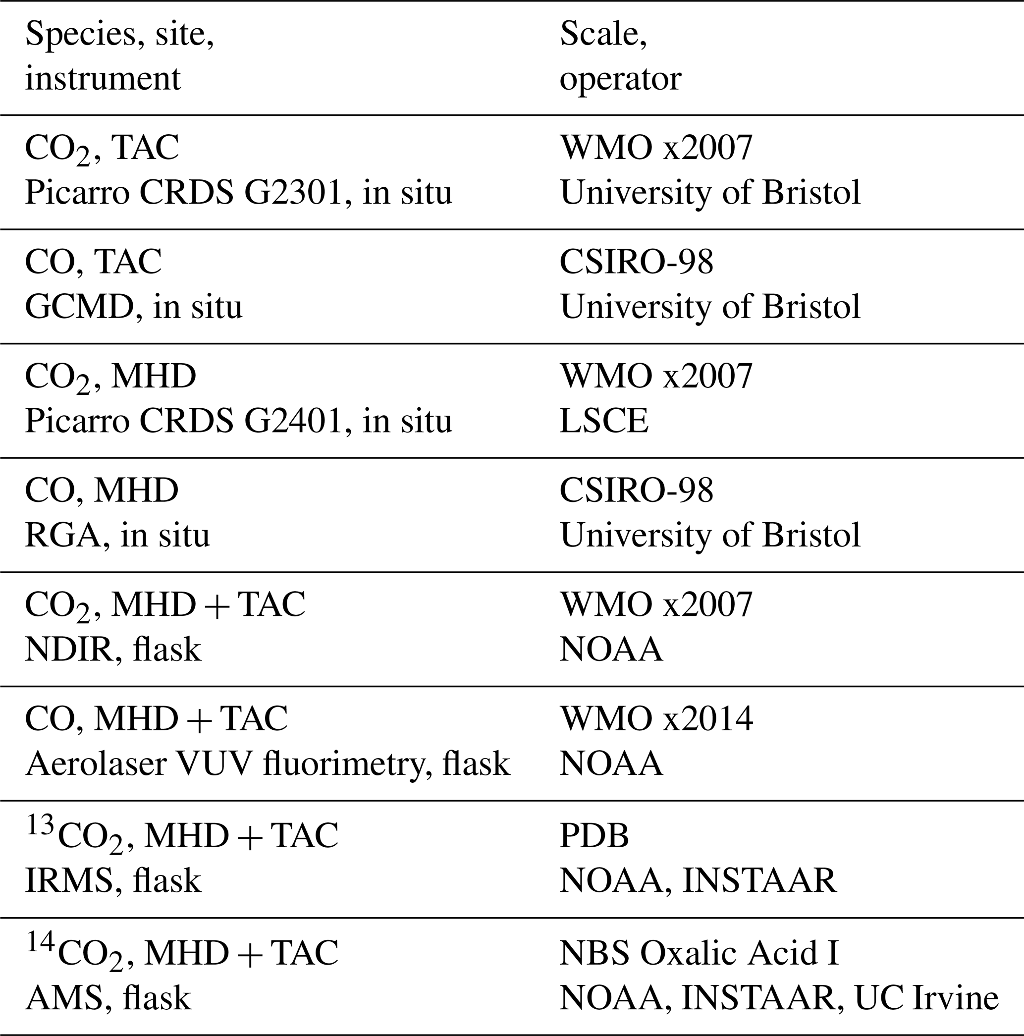
The TAC tall tower measurement site was set up in 2012 as part of the UK DECC (Deriving Emissions linked to Climate Change) network (Fig. 1). It is operated by Bristol University and the University of East Anglia. More details on the site and the network have been previously published (Stanley et al., 2018). The site is located in Norfolk, approximately 140 km north-east of London. It was thought to be the most appropriate site in the UK DECC tall tower network for characterizing ffCO₂ emissions from the UK using ¹⁴CO₂ because it has the most influence from fossil fuel sources and the least influence from nuclear power stations. The TAC tower site has three inlet heights: 54, 100, and 185 m. CO is observed from the 100 m inlet once every 20 min. The CO₂ observations are reported as 1 min means and all heights were sampled at an interval of 20 min per height. The highest height (185 m) was used for the ¹⁴CO₂ measurements as it was assumed that it would be the most representative for well-integrated air masses. A background observation is necessary for the ¹⁴CO₂ method to evaluate the relative depletion caused by recently added emissions of ffCO₂. Different types of sites have been utilized as background in previous studies: relatively unpolluted sites upwind of significant fossil fuel CO₂ sources (Lopez et al., 2013), high-altitude observations (Bozhinova et al., 2014; Levin and Kromer, 1997), free troposphere observations from an aircraft (Miller et al., 2012; Turnbull et al., 2011), and a mildly polluted site upwind of the polluted site (Turnbull et al., 2015). MHD, located on the west coast of Ireland, was used as the background site for this study and weekly sampling was performed when air masses were representative of clean air coming from the Atlantic (Fig. 1). This study utilized both flask and, for some species, high-frequency in situ data from two sites (MHD and TAC), Table 1 gives an overview of the measurement techniques used, the calibration scales, and the operator of the specific instrument or method. For CO, the flask and the in situ data were reported on different calibration scales. Comparisons of co-located observations at MHD show that there is a significant difference between the two scales (Fig. S1 in the Supplement). Conversion between the CSIRO-98 and the WMO-2014 CO scale is non-trivial as there is a time and concentration dependent difference between the two scales and no published conversion method is yet available. It was decided that only the in situ data would be utilized for the CO ratio analysis to avoid any effect these calibration scale differences might have on the CO ratio analysis. At TAC, the in situ CO observations (100 m) were made at a different height to the flask sampling (185 m). Observations of CH₄ and CO₂ at the two heights were similar (less than 0.4 % difference) within the same hour the flasks were taken, indicating that it was acceptable to use the CO observations at 100 m. A comparison of the concentration of CH₄ and CO₂ in the flask samples vs. the respective time-matched in situ observations at 185 m showed good agreement (less than 0.2 % difference). The measurements are reported as dry air mole fractions in ppm (µmol mol⁻¹) and ppb (nmol mol⁻¹).

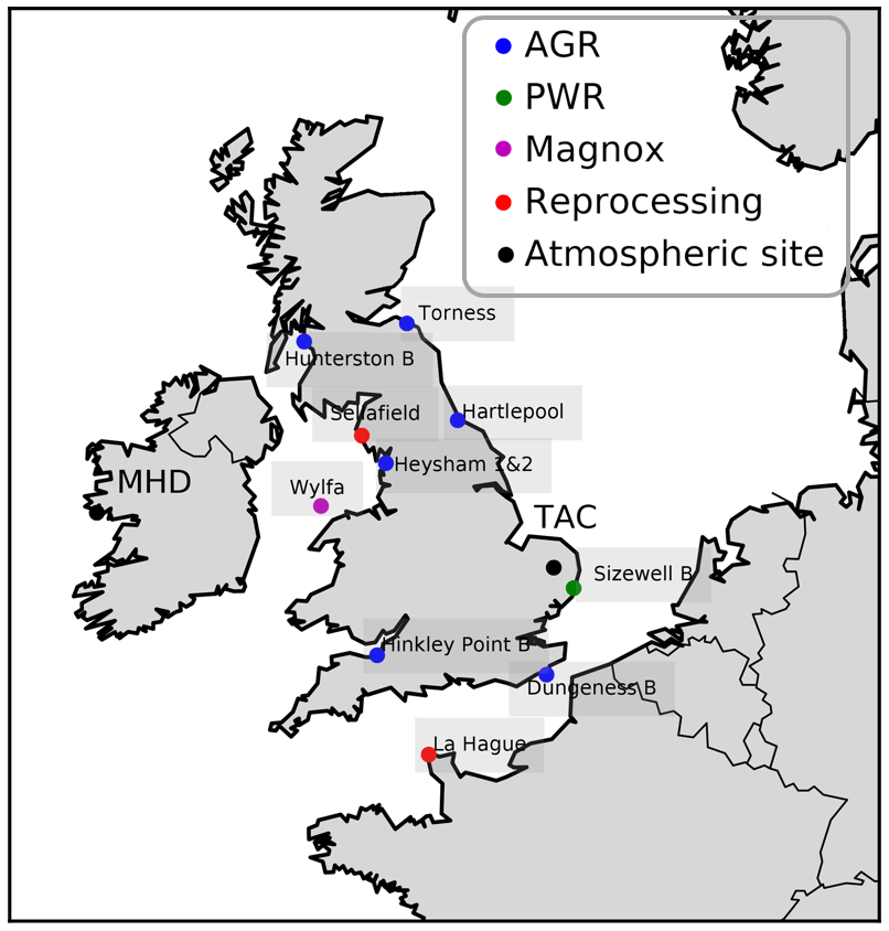
Figure 1 Map of north-western Europe nuclear power stations and other nuclear facilities. Reactor types are the advanced gas-cooled reactor (AGR) (blue), pressurized water reactor (PWR) (green), and Magnox (pink). Fuel reprocessing sites are labelled separately (red). The atmospheric measurement sites (Tacolneston, TAC, and Mace Head, MHD) are also labelled (black).

Table 1 Overview of greenhouse gas measurements presented in this paper. The acronyms used to describe instruments are cavity ring-down spectroscopy (CRDS), gas chromatography mass detector (GCMD), residual gas analyser (RGA), nondispersive infrared detector (NDIR), vacuum ultra violet (VUV) infrared mass spectrometer (IRMS), and accelerator mass spectrometer (AMS).

2.2 Sampling

The sampling procedure was based on the method used by the National Oceanic and Atmospheric Administration Carbon Cycle Greenhouse Gases (NOAA CCGG; Lehman et al., 2013). At MHD, the sampling of an additional flask for ¹⁴CO₂ analysis was added to the existing weekly NOAA CCGG flask sampling collection. A manual instantaneous sampling module was constructed for TAC, using a KNF pump to pressurize and a Stirling cooler (Shinyei MA-SCUCO8) set to 0 ^∘C to dry the sample. Additionally, a 7 µm particle filter was added to avoid contamination of the sampling module, and a check valve in addition to a toggle valve were added to ensure that existing measurements at the site were not influenced. A selection of tests, including a side-by-side comparison with the NOAA CCGG sampling unit at MHD, was performed before deployment to TAC. At TAC, samples were collected weekly into 2 L glass flasks (NORMAG, Germany, based on the NOAA CCGG design).

3 Methods

3.1 NAME simulations

Mole fractions were simulated at each measurement site using the Lagrangian particle dispersion model NAME (Numerical Atmospheric dispersion Modelling Environment) developed by the UK Met Office (Jones et al., 2007). Hypothetical particles are released into the model atmosphere at a rate of 10 000 per hour at the location of the observation site and transported backward in time for 30 d. It is assumed that when a particle resides in the lowest 0–40 m of the model atmosphere, pollution from ground-based emission sources is added to the air parcel (Arnold et al., 2018; Manning et al., 2011). The particle residence times in this surface layer are integrated over the 30 d simulation to calculate a “footprint” of each measurement that quantifies the sensitivity of the observation to a grid surrounding the measurement site (Manning et al., 2011). These footprints can be multiplied by flux fields to simulate the mole fraction due to each source at each instant in time. An example of such a footprint, also called back trajectory, can be found in the Supplement (Fig. S2). In a similar fashion the NAME model can be run forward in time to simulate the concentration of a substance in the modelling domain. To simulate the concentration of a substance in the modelling domain, theoretical particles are released at the emission source location (point sources and area sources) with a rate that is relative to the emission source strength. We separate the CO₂ mole fraction into a background concentration CO_2, bg and a contribution from each source i:

$$\begin{array}{}\text{(1)}& {\mathrm{CO}}_{\mathrm{2}}={\mathrm{CO}}_{\mathrm{2},\mathrm{bg}}+\sum _i{\mathrm{CO}}_{\mathrm{2},\mathit{\text{i}}}.\end{array}$$

The background concentration can be determined by applying statistical methods to high-frequency observations (Barlow et al., 2015; Ruckstuhl et al., 2012) or estimated by models (Balzani Lööv et al., 2008; Lunt et al., 2016). In this work, high-frequency data existed only for ¹²CO₂ but not its isotopes and there was no model-derived background available for the isotopes; therefore, MHD data were used as background for the simulation of all CO₂ isotopes. While ¹³CO₂ and ¹⁴CO₂ measurements at MHD were selectively sampled during clean air conditions (high wind speeds from the Atlantic Ocean), the high-frequency ¹²CO₂ data also contained pollution events. To exclude the pollution events, a rolling 15th percentile value (±20 d) was calculated and used as ¹²CO₂ background. The 15th percentile of the MHD data was chosen for the background curve over other percentiles because it successfully removed short-term concentration changes and pollution events. In addition to creating a smooth curve, the 15th percentile of the MHD data also fitted low concentrations observed in TAC, outside of the growing seasons (not much CO₂ uptake due to photosynthesis), well. Similarly, for the ¹³CO₂ and ¹⁴CO₂ background, rolling median values (±30 d) were calculated. These rolling median values created a smoother seasonal cycle compared to using the closest observed value.

3.2 Isotope modelling

This section describes the method and the equations used to model ¹²CO₂, ¹³CO₂, and ¹⁴CO₂ at TAC. The modelling of the two stable CO₂ isotopes was necessary in order to be able to simulate the ¹⁴CO₂. A framework to simulate ¹⁴CO₂ was developed as a tool to investigate the observations and possible constraints of the radiocarbon method. A basic mass balance (Eq. 1) was used as the basis of the modelling, where the observed atmospheric mole fraction of CO_2 obs can be described as the sum of CO₂ from individual sectors (CO_2 i) and a background contribution. This simple concept was adapted to the different CO₂ isotopes by using the definition of the small delta (δ) value for ¹³CO₂ and the definition of the large delta (Δ) ¹⁴CO₂ as defined in Stuiver and Polach (1977). The simulated ¹³CO₂ was calculated with Eq. (2) and the Δ¹⁴CO₂ with Eqs. (3a), (3b). A detailed description on how Eqs. (2), (3a) and (3b) were derived can be found in Sect. S1 in the Supplement.

$$\begin{array}{}\text{(2)}& \begin{array}{rl}{\mathit{\delta }}^{\mathrm{13}}{\mathrm{CO}}_{\mathrm{2}}& =\left({\displaystyle \frac{\frac{\sum \left(\left(\frac{{\mathit{\delta }}^{\mathrm{13}}{\mathrm{CO}}_{\mathrm{2},\mathit{\text{i}}}}{\mathrm{1000}}+\mathrm{1}\right)\times {}^{\mathrm{12}}{\mathrm{CO}}_{\mathrm{2}\mathit{\text{i}}}{\times }^{\mathrm{13}}{R}_{\mathrm{std}}\right)+{}^{\mathrm{13}}{\mathrm{CO}}_{\mathrm{2},\mathrm{bg}}}{{}^{\mathrm{12}}{\mathrm{CO}}_{\mathrm{2}}}}{{}^{\mathrm{13}}{R}_{\mathrm{std}}}}-\mathrm{1}\right)\\ & \times \mathrm{1000}.\end{array}\end{array}$$

Here, δ¹³CO_2 i is the ¹³CO₂ signature of emission source sector i (‰); ¹³CO_2 bg is the background ¹³CO₂ abundance from the rolling (±30 d) median values of the MHD observations, ¹²CO_2, i is equal to abundance of ¹²CO₂ from sector i (mol mol⁻¹) as simulated in TAC (Eq. 1); ¹³R_std is the ratio of reference standard ((mol mol⁻¹) ∕ (mol mol⁻¹)); and ¹²CO₂ is the total ¹²CO₂ enhancement (mol mol⁻¹) from Eq. (1).

$$\begin{array}{}\text{(3a)}& {\displaystyle }X={\displaystyle \frac{\sum \left(\frac{\left(\frac{{\mathrm{\Delta }}^{\mathrm{14}}{\mathrm{CO}}_{\mathrm{2},\mathit{\text{i}}}}{\mathrm{1000}}+\mathrm{1}\right){\times }^{\mathrm{14}}{R}_{\mathrm{std}}}{\mathrm{1}-\mathrm{2}\times \frac{\mathrm{25}+{\mathit{\delta }}^{\mathrm{13}}{\mathrm{CO}}_{\mathit{\text{i}}}}{\mathrm{1000}}}\times {}^{\mathrm{12}}{\mathrm{CO}}_{\mathrm{2},\mathit{\text{i}}}\right)}{{}^{\mathrm{12}}{\mathrm{CO}}_{\mathrm{2}}}}\text{(3b)}& {\displaystyle }{\mathrm{\Delta }}^{\mathrm{14}}{\mathrm{CO}}_{\mathrm{2}}=\left({\displaystyle \frac{X\times \left(\mathrm{1}-\mathrm{2}\cdot \frac{\mathrm{25}+{\mathit{\delta }}^{\mathrm{13}}{\mathrm{CO}}_{\mathrm{2}}}{\mathrm{1000}}\right)}{{}^{\mathrm{14}}{R}_{\mathrm{std}}}}-\mathrm{1}\right)\times \mathrm{1000},\end{array}$$

where Δ¹⁴CO_2, i is the ¹⁴CO₂ signature of emission source sector i (‰), ¹²CO_2 i is the abundance of CO₂ from sector i (mol mol⁻¹) from Eq. (1), ¹⁴R_std is the ratio of reference standard ((mol mol⁻¹) ∕ (mol mol⁻¹)), ¹²CO₂ is the total CO₂ mole fraction0 (mol mol⁻¹) from Eq. (1); and δ¹³CO₂ is the ¹³CO₂ signature (‰) from Eq. (2).

The Δ¹⁴C is normalized to a δ¹³C value of −25 ‰; this is done to account for fractionation of the sample. Fractionation is the discrimination against one isotope in favour of the other in physical processes and chemical reactions. This discrimination takes place as the additional neutron in ¹³C alters both the weight of the carbon and their chemical bonding energies. Biological processes such as, for example, photosynthesis selectively favour the lighter isotope. Fractionation effects discriminate against ¹⁴C approximately twice as much as for ¹³C (Fahrni et al., 2017; Stuiver and Polach, 1977). Normalizing δ¹⁴C measurements to a common δ¹³C removes reservoir-specific differences that are caused by fractionation.

For this work, sector-specific emissions reported in EDGAR v4.2 from the year 2010 (Olivier et al., 2014) were used for the simulations of anthropogenic emissions and the National Aeronautics and Space Administration Carnegie Ames Stanford Approach (NASA CASA) emissions for biogenic emissions (Potter, 1999). It is assumed that all emissions reported in EDGAR correspond to ¹²CO₂ emissions. A detailed list of source sectors and associated isotopic signatures can be found in the Supplement (Table S1). All fossil sources were considered to have a Δ¹⁴CO₂ value of −1000 ‰.

3.3 Determination of fossil fuel CO₂ with Δ¹⁴CO₂ observations

The Δ¹⁴CO₂ observations at TAC and MHD were used to calculate the recently added CO₂ from fossil fuel burning (ffCO₂). This method takes advantage of the fact that fossil fuels have been isolated from other carbon pools for so long that they are completely devoid of ¹⁴C; recent additions of CO₂ from fossil fuel burning therefore lead to a depletion in the atmospheric Δ¹⁴CO₂. We followed the approach of Turnbull et al. (2009a); this approach was chosen as the calculation of the uncorrected ffCO₂ is separated from the corrections. This means that each correction can be evaluated for its impact on the final ffCO₂ value individually. The equation given in Turnbull et al. (2009a) was adapted to have a correction term for heterotrophic respiration (Sect. 3.3.1) and emissions from the nuclear industry (Sect. 3.3.2), and is given in Eq. (4). The reasoning behind the need for the corrections for heterotrophic respiration and emissions from the nuclear industry are explained in detail in the next two sections.

$$\begin{array}{}\text{(4)}& \begin{array}{rl}{\mathrm{CO}}_{\mathrm{2}\mathrm{ff}}& ={\displaystyle \frac{{\mathrm{CO}}_{\mathrm{2},\mathrm{bg}}({\mathrm{\Delta }}_{\mathrm{obs}}-{\mathrm{\Delta }}_{\mathrm{bg}})}{({\mathrm{\Delta }}_{\mathrm{ff}}-{\mathrm{\Delta }}_{\mathrm{obs}})}}-{\displaystyle \frac{{\mathrm{CO}}_{\mathrm{2}\mathrm{hr}}({\mathrm{\Delta }}_{\mathrm{hr}}-{\mathrm{\Delta }}_{\mathrm{obs}})}{({\mathrm{\Delta }}_{\mathrm{ff}}-{\mathrm{\Delta }}_{\mathrm{obs}})}}\\ & -{\displaystyle \frac{{\mathrm{CO}}_{\mathrm{2}\mathrm{nuc}}({\mathrm{\Delta }}_{\mathrm{nuc}}-{\mathrm{\Delta }}_{\mathrm{obs}})}{({\mathrm{\Delta }}_{\mathrm{ff}}-{\mathrm{\Delta }}_{\mathrm{obs}})}}\end{array}\end{array}$$

Here CO_2 ff describes the recently added mole fraction from fossil fuel burning. CO_2 bg describes the background mole fraction. The rolling 15th percentile value (±20 d) of the high-frequency CO₂ observations at MHD (background site) was used as CO_2 bg. For the Δ_bg, the rolling median value of the Δ¹⁴CO₂ flask measurements at MHD were calculated within a time window of ±20 d of the Δ_obs. Figure S6 in the Supplement shows the MHD Δ¹⁴CO₂ observations and the rolling median value of the data used as Δ_bg. The use of the 15th percentile for the high-frequency CO₂ data and the median for the Δ¹⁴CO₂ for weekly flask sampling (targeting background conditions) is consistent with the values used in the Δ¹⁴CO₂ modelling in Sect. 3.1. CO_2 obs corresponds to the observed CO₂ mole fraction in the flask measurements at TAC (polluted site), while Δ_obs refers to the Δ¹⁴CO₂ measured from those same flasks. The Δ_ff describes the ¹⁴CO₂ signature of fossil fuel burning, and this was assumed to be −1000 ‰. Equation (4) also contains two correction terms, one for nuclear emissions and one for heterotrophic respiration. In addition to these two correction terms explained below, other work (Graven et al., 2012; Turnbull et al., 2009b) investigated corrections for cosmogenic ¹⁴C production and for the ocean–atmosphere CO₂ exchange. For our work, both the ocean–atmosphere CO₂ exchange and the cosmogenic ¹⁴C production were considered negligible as the corrections are generally small and not trivial to model. CO_2 hr corresponds to the mole fraction of CO₂ at TAC that originates from heterotrophic respiration, while the Δ_hr is the Δ¹⁴CO₂ signature of heterotrophic respiration; both values were obtained by models as described in Sect. 3.3.1. The Δ_nuc is the Δ¹⁴CO₂ signature of pure ¹⁴CO₂ emissions (${\mathrm{\Delta }}_{\mathrm{nuc}}\approx \mathrm{7.3}\times {\mathrm{10}}^{\mathrm{14}}$ ‰; Bozhinova et al., 2014) from nuclear sites and CO_2 nuc is the mole fraction of CO₂ from nuclear emission at TAC (this value is obtained by modelling as described in Sect. 3.3.2). It is important to note that all approaches used to determine ffCO₂ from Δ¹⁴CO₂ observations make certain assumptions; the method used here and described in detail in Turnbull et al. (2009a) assumes that CO₂ emitted from autotrophic respiration has the same Δ¹⁴CO₂ signature as the observations (Δ_obs); Sect. 3.3.1 goes into more detailed as to why this is a reasonable assumption to make. All values used in the calculation of CO_2 ff, including the Δ_obs, and the Δ_bg and the correction terms have been included in Table S3.

3.3.1 Biospheric correction

In the 1950s and 1960s extensive nuclear weapon tests caused a sudden sharp increase in the atmospheric ¹⁴CO₂ content; this is commonly referred to as the bomb spike (Levin et al., 1980; Manning et al., 1990). This bomb ¹⁴CO₂, has gradually been assimilated into other carbon pools (see Fig. S3 in the Supplement). Carbon that is exchanged from the biosphere to the atmosphere can have a different Δ¹⁴CO₂ signature depending on when the carbon was originally assimilated into the biosphere. To account for this, biospheric emissions were split into two sources, autotrophic and heterotrophic. Autotrophic respiration of plants generally contains recently assimilated carbon (<1 year). Therefore, ¹⁴CO₂ from autotrophic respiration is generally assumed to be in equilibrium with the atmosphere. While recent work has indicated that autotrophic respiration may also contain older carbon (Phillips et al., 2015), it is assumed to be negligible for this work. Heterotrophically respired CO₂ contains carbon from older pools (for example decaying biomass) and can be significantly enriched in ¹⁴C compared to current atmospheric CO₂ (Naegler and Levin, 2009). To simulate the Δ¹⁴CO₂ from heterotopic respiration, the 1-box model developed by Graven et al. (2012) was used; it is assumed that two-thirds of heterotrophic respiration originates from older carbon pools. This resulted in a Δ¹⁴CO_2HR of 67 ‰–91 ‰ for 2014–2015. For the calculation of ffCO₂ with Eq. (4), 80 ‰ was used as the ¹⁴CO₂ signature of heterotrophic respiration (Δ_HR). The mole fraction enhancement due to CO₂ emitted from heterotrophic respiration (CO_2 HR) was derived from the NASA CASA biosphere model and atmospheric back trajectories (more details about the modelling can be found in Sect. 3.1). A similar disequilibrium exists between the atmosphere and the ocean, but it was considered negligible for this work.

3.3.2 Nuclear correction

Radiocarbon emissions from nuclear reactors have a large temporal variability, making them difficult to correct for. Although the emissions are small, they have a Δ¹⁴C value of $\sim \mathrm{7.3}\times {\mathrm{10}}^{\mathrm{14}}$ ‰ and can therefore influence radiocarbon observations significantly. During the study period, three types of nuclear power plants were in operation in the UK (Fig. 1). Of these, both the AGR and the Magnox reactor are cooled with CO₂ gas. This creates an oxidizing condition in the reactor, resulting in the majority of the released ¹⁴C being released in the form of ¹⁴CO₂. ¹⁴C is produced in the reactor from reactions of neutrons with ¹⁴N, ¹³C, and ¹⁷O. Most of the ¹⁴CO₂ emitted from the AGRs and Magnox plants originate from N₂ impurities in the cooling gas (Yim and Caron, 2006). The UK also has one running pressurized water reactor (PWR), Sizewell B (52.21^∘ N, 1.62^∘ E), in the east of England. PWRs contain a reducing reactor environment, leading to ¹⁴C being released predominantly in the form of ¹⁴CH₄. As ¹⁴C is constantly produced in nuclear reactors, parameterized emissions (an average emission factor per plant type that is multiplied with the power production of a plant) are a good approximation. However, the production of ¹⁴C is highly dependent on the number of impurities present in the reactor and only a small part of the produced ¹⁴C is ever emitted. Emissions can be caused by leakage as well as operational procedures, known as blowdown events. Reported emissions are therefore more informative. To apply a correction for these nuclear industry emissions in the calculation of ffCO₂ in Eq. (4), 7.3×10¹⁴ ‰ was used as the Δ_nuc. To calculate the mole fraction of CO₂ derived from the nuclear industry (CO_2 nuc in Eq. 4), atmospheric back trajectories were multiplied with a ¹⁴CO₂ emission map of reported nuclear industry emissions that was especially created for this study. This ¹⁴CO₂ emissions map was created with the highest-frequency data available from each nuclear site. Monthly atmospheric emission data were provided by the two operators of the 10 UK nuclear power plants; EDF (Électricité de France) and Magnox Ltd. Data for the other 17 UK nuclear sites were taken from the annual Radioactivity in Food and the Environment RIFE, 1995–2016 (Environment Agency, Natural Resources Wales, 2017). The emissions from other European nuclear power plants were sourced from annual environmental reports if available (France, Germany); otherwise, parameterized emissions were calculated according to Graven and Gruber (2011). The largest emitter of ¹⁴C during the study period was the nuclear fuel reprocessing site in La Hague, northern France (49.68^∘ N, 1.88^∘ W). For the nuclear fuel reprocessing site in La Hague, monthly emission data reported on their website were utilized; a table transcribing these reported emissions is included in the Supplement (Table S2).

4 Results

4.1 Comparison of modelled and observed data

For this work ¹²CO₂, δ¹³CO₂, and Δ¹⁴CO₂ were simulated using Eqs. (1), (2), (3a) and (3b) at TAC and are compared with observations in Fig. 2. Daily mean values (24 h) are displayed for both the modelled (blue line) and the observed data (black line, points). The uncertainty estimate (light blue area) includes the baseline uncertainty as well as the emission inventory uncertainty. The uncertainties were investigated by calculating a Monte Carlo ensemble of model runs (4000 runs) with perturbed background concentrations and sector-specific emissions. The background concentration was randomly altered within a factor of 2 of the measurement uncertainty. The sector-specific emission maps were multiplied with a randomly generated matrix that let the emission in each grid cell vary between 50 % and 150 %. The shaded green areas represent the 95 % confidence interval uncertainty of these simulations. The TAC observations generally match the simulations well for ¹²CO₂ and ¹⁴CO₂. The exception is a large ¹²CO₂ peak in November 2014 that is significantly underestimated by the model. During the same time period, the two ¹⁴CO₂ samples taken were more depleted than the ¹⁴CO₂ simulations.

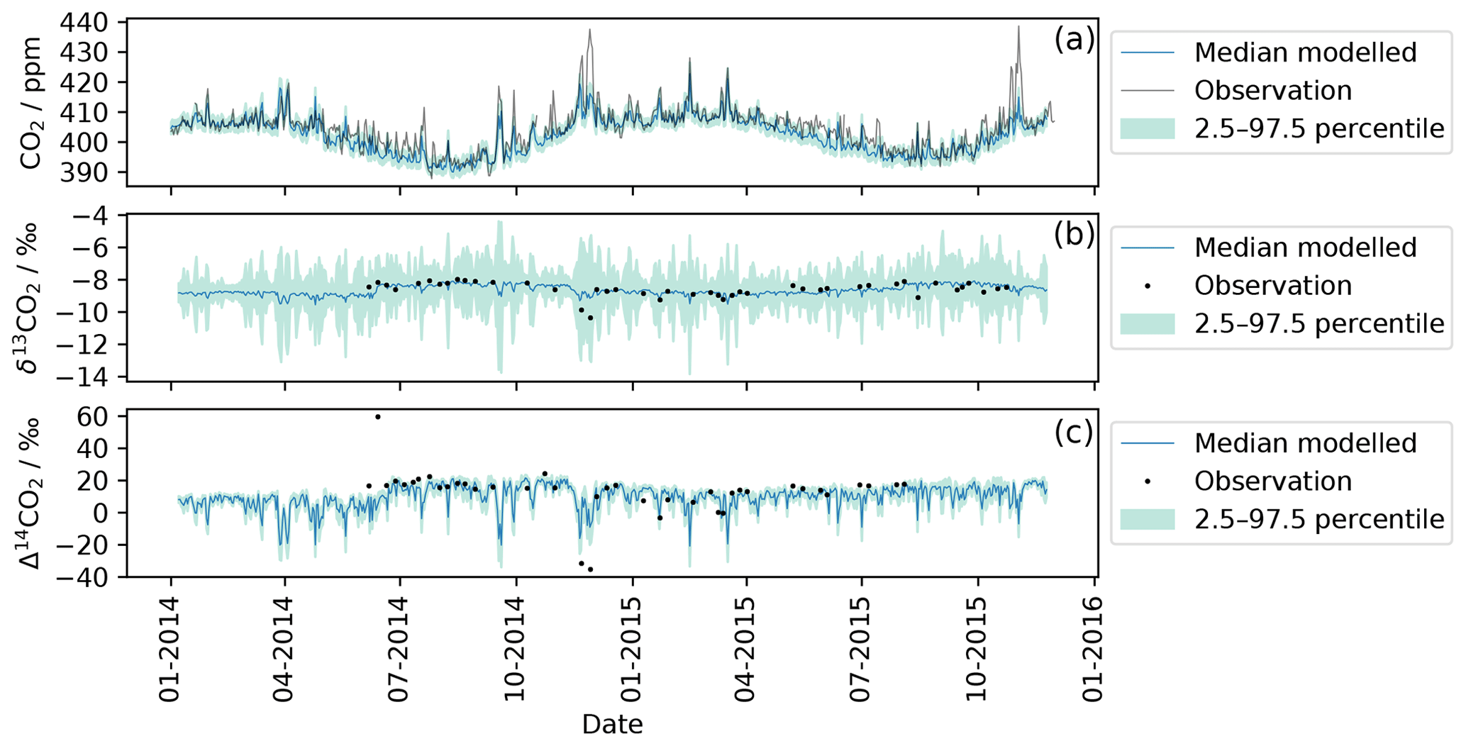
Figure 2 Comparison of modelled and observed CO₂ for each isotope at TAC. The black line and dots represent observations measured at the TAC field station. The blue line corresponds to the median modelled value (according to Sect. 3.2). The shaded green area represents the uncertainty estimate for the modelled values based on the bootstrapping method described in Sect. 4.1. Panel (a) compares observed and modelled ¹²CO₂ values. Panel (b) contains both modelled ¹³CO₂ and flask-sampling-based observations, while (c) shows the modelled and observed ¹⁴CO₂ data.

The δ¹³CO₂ simulations (Fig. 2) show comparatively large uncertainties; this uncertainty is dominated by the variation in the net ecosystem exchange flux (from NASA CASA) during the Monte Carlo runs described above. The variation in the net ecosystem exchange flux has an ostensibly larger influence on the ¹³CO₂ simulations (compared to the ¹²CO₂ and ¹⁴CO₂) as carbon uptake and respiration cause strong fractionation in the atmosphere. This fractionation was captured in the model and the uncertainty estimation by assigning a δ¹³CO₂ signature to the net ecosystem exchange flux (see Eq. 2 in Sect. 3.2 and Table S1 in the Supplement). The close fit of the observations to the median of the simulations indicates that the variability in the δ¹³CO₂ signature of the net ecosystem exchange flux might have been overestimated.

For the ¹⁴CO₂ simulations as shown in Fig. 2, the calculated uncertainty estimate was ±5 ‰ or ∼1.8 ppm in ffCO₂ equivalent. The term fossil fuel equivalent is used to describe how much recently emitted fossil fuel would have to be present in a sample to cause the equivalent depletion in ¹⁴C in per mille (‰); the exact conversion from one to the other depends on the current atmospheric background level of CO₂ and its isotopes. The uncertainty estimate of $>\pm \mathrm{5}$ ‰ was predominantly influenced by the uncertainty in the ¹⁴CO₂ background value, as this was chosen to be double the measurement uncertainty ($>\pm \mathrm{4}$ ‰). This is not surprising as the Δ¹⁴CO₂ observations have a large measurement uncertainty (1.8 ‰, ∼0.72 ppm ffCO₂ equivalent) associated with them, and the measurement uncertainty was chosen as an indication of the background uncertainty. However, it emphasizes that strong ffCO₂ signals are needed in order to obtain Δ¹⁴CO₂ observations that can be distinguished from the background. At TAC, the fossil fuel influence is not always large enough to exceed this threshold.

4.2 Fossil fuel CO₂ derived from Δ¹⁴CO₂ observations

This paper aims to determine if Δ¹⁴CO₂ observations can be used to estimate ffCO₂ at the TAC observation station in the UK. Multiple studies (Bozhinova et al., 2014; Graven and Gruber, 2011) have indicated that in some parts of the UK the radiocarbon method cannot be used as the large ¹⁴CO₂ emissions from nuclear sites would mask the depletion in the atmospheric Δ¹⁴CO₂ caused by recent fossil fuel emission. The flask sampling site in TAC was chosen deliberately following a preliminary study that suggested the influence from ¹⁴CO₂ from the nuclear industry at the TAC was moderate.

4.2.1 Influence of the corrections applied to the ffCO₂ calculation

During the calculation of the ffCO₂ with Eq. (4), two correction terms were applied, one for heterotrophic respiration and one for the ¹⁴CO₂ emissions from the nuclear industry. The correction for heterotrophic respiration has to be applied at any site that could be influenced by biospheric fluxes (biospheric correction), while only sites located within the influence of nuclear industry sites have to apply the correction from nuclear industry emissions (nuclear correction). The biospheric and nuclear corrections were calculated using Eq. (4) and as outlined in Sect. 3.3.1 and 3.3.2. In Fig. 3, the biospheric and nuclear corrections were calculated for the whole study period (2014–2015). To facilitate the comparison of their impact on the final ffCO₂ correction, both the biospheric correction and the nuclear correction are displayed in ffCO₂ equivalent (unit of the individual correction terms in Eq. 4). The points in Fig. 3 represent times when flask samples were taken at TAC. Since we aim to assess if TAC is a suitable site to derive ffCO₂ from Δ¹⁴CO₂ observations, the influence of the nuclear and biospheric corrections were assessed for the whole study period. The mean of the correction applied was 0.34 ppm ffCO₂ equivalent for the heterotrophic respiration and 0.25 ppm for the nuclear emissions. This means that the average nuclear correction over the whole study period at TAC for radiocarbon-derived ffCO₂ is similar in magnitude to the correction for heterotrophic respiration. The maximum value calculated for the nuclear correction was 1.60 ppm ffCO₂ equivalent, similar to the highest biospheric correction value (1.23 ppm). For the nuclear correction, the fuel reprocessing site in La Hague and the nuclear power plant in Sizewell have the largest influence on the air parcels arriving at TAC: the fuel reprocessing site in La Hague because it is the highest ¹⁴C emitter, and the nuclear power plant in Sizewell as it is spatially close, 50 km south-east of TAC.

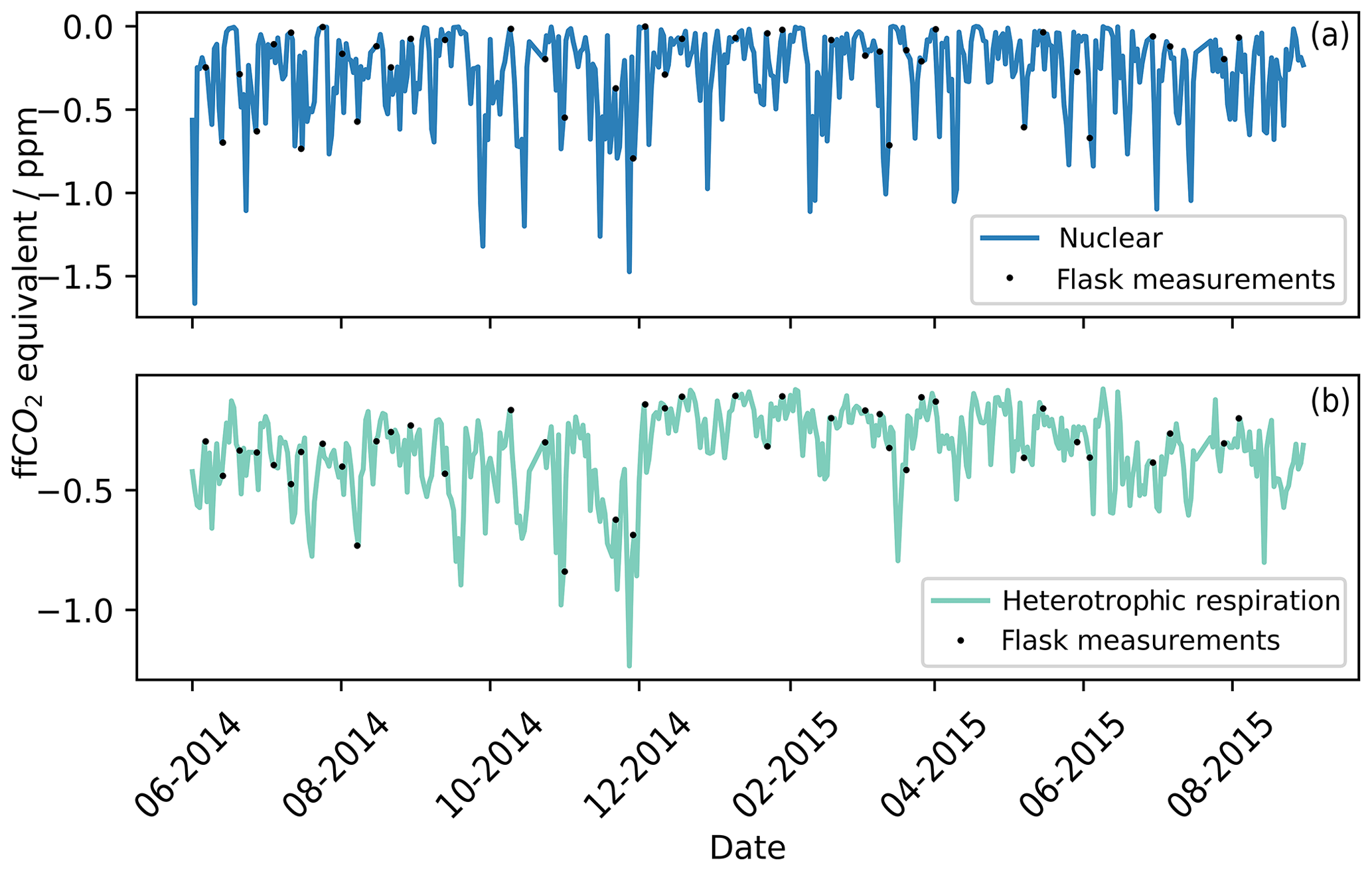
Figure 3 The blue line (a) represents the ffCO₂ equivalent theoretical corrections that need to be applied over the whole study period for the nuclear ¹⁴CO₂ emissions (see Sect. 3.3.2). The green line (b) represents the ffCO₂ equivalent theoretical corrections that need to be applied over the whole study period for heterotrophic respiration from the biosphere (see Sect. 3.3.1). The black points represent times that flask samples were taken and therefore the corrections that were applied to each flask measurement.

The average corrections applied for the heterotrophic respiration and the nuclear industry emissions are much smaller than the combined measurement uncertainty in the radiocarbon method to calculate ffCO₂ (±5 ‰ ∼ 1.8 ppm ffCO₂ equivalent). The observed ffCO₂ signal in TAC is frequently (50 % of observations) smaller than the measurement uncertainty in the radiocarbon method. Note that the nuclear correction is based on reported monthly emission data from the operational UK nuclear power plants (Sect. 3.3.2). This temporal resolution does not capture complete reactor blowdowns before maintenance shutdowns of nuclear power plants. The ¹⁴CO₂ emissions during these blowdown events can be 10 times higher than during standard operation. It is our opinion that these larger emissions before reactor maintenance are the cause of the very enriched data point of over 50 ‰ (Fig. 3) on the 13 June 2014. The size of the nuclear correction calculated for the 13 June 2014 was 0.017 ppm; this obviously severely underestimates the nuclear enhancement observed in the sample. Back trajectories associated with this sample (Fig. S2) show that air masses originated from the north-west of England, where two nuclear power plants (Heysham 1&2; 54.03^∘ N, 2.92^∘ W) and a nuclear fuel processing site (Sellafield; 54.42^∘ N, 3.50^∘ W) are situated. Heysham 1 was shutdown for an in-depth boiler inspection (Office for Nuclear Regulation, 2014) on the 10 June 2014; emissions caused by this shutdown could potentially explain the high Δ¹⁴CO₂ value observed on the 13 June 2014 at TAC.

4.2.2 Results of ffCO₂ derived from Δ¹⁴CO₂ observations at TAC

This section presents the results of the radiocarbon method that were gained from the Δ¹⁴CO₂ measurements performed at the TAC and MHD observation sites. All the data presented in this section are available on the Centre for Environmental Data Analysis (CEDA) database (http://data.ceda.ac.uk/badc/gauge/data/tower/, last access: 9 May 2019). In Fig. 4 we present the ffCO₂ calculated with the radiocarbon method (Eq. 4) from Δ¹⁴CO₂ observations at the TAC station (ffCO_2 observed) and compare it with simulated mixing ratios derived from modelling using emission inventories as described in Sect. 3.1 (ffCO_{2 simulated}). A value of 1 ppm of ffCO₂ causes a depletion of approximately 2.5 ‰ in Δ¹⁴CO₂. Figure 4 shows that most observed values are not significantly different from the modelled values. This implies that the ffCO₂ derived from Δ¹⁴CO₂ observations at TAC agrees well with the values simulated using emissions inventories (EDGAR 2010) and an atmospheric model (Sect. 3.2). However, the uncertainties associated with the observed ffCO₂ are relatively large, while the ffCO₂ mole fractions observed at TAC are comparatively low.

Figure 4 Comparison of fossil fuel CO₂ (observed ffCO₂) derived from Δ¹⁴CO₂ measurements made at TAC (Sect. 3.3, Eq. 4) compared to simulated ffCO₂. The simulated ffCO₂ was calculated from NAME model back trajectories and the EDGAR 2010 fossil fuel emission inventory according to Sect. 3.1. Observations that have been corrected for nuclear (Sect. 3.3.2) and biospheric (Sect. 3.3.1) influences are shown as blue points, whereas the uncorrected values are shown as green crosses. The 1:1 line shown in black represents the theoretical line where observed data match the simulated values and therefore the emission inventory exactly. The linear regression lines for the comparison of the modelled ffCO₂ to the corrected and uncorrected observed ffCO₂ are shown as blue and green lines, respectively. Error bars are 1.8 ppm.

The very enriched Δ¹⁴CO₂ value observed on the 13 June 2014 was excluded from this analysis; this sample was likely influenced by ¹⁴CO₂ emissions from a nuclear reactor shutdown as explained in Sect. 4.2.1. Figure 2 shows two other values that were excluded, both in November 2014. These observations were strongly depleted in ¹⁴CO₂ and coincided with a CO₂ enhancement that lasted approximately 2 weeks. Footprints calculated during this period indicate that the high CO₂ abundance observed is associated with an accumulation of emissions from a large geographical area over the UK and north-west Europe, due to an extended period of low wind speeds, during which the model appears to significantly underestimate the amplitude of the CO₂ peak. The two Δ¹⁴CO₂ measurements taken during this period were excluded from further analysis for two reasons: firstly because the ffCO₂ signal of those two points is so strong that it distorts the interpretation of all the other observations and secondly because it is likely that the model would not represent the conditions during that period well (in an extended period of low wind speeds the modelled wind speed and direction have considerable uncertainty and variability due to the dominant influence of local terrain features that are sub-grid scale and therefore not resolved).

4.2.3 Increasing the temporal resolution of ffCO₂ using CO ratios

Carbon monoxide (CO) is a product of incomplete combustion and as such is co-emitted with the CO₂ produced by complete combustion. CO emissions can be expressed as a ratio relative to the fossil fuel CO₂ emissions. The emitted CO∕CO₂ ratio varies depending on the emission source. According to the National Atmospheric Emissions Inventory (NAEI) 2014, UK gas power plants (1.0 ppb (CO) ppm (CO₂)⁻¹) and cars (0.5 ppb (CO) ppm (CO₂)⁻¹) under ideal driving conditions have low emission ratios, while larger vehicles preforming a cold start or accelerating on the motorway can have an emission factor an order of magnitude larger. Δ¹⁴CO₂-derived ffCO₂ is an expensive measurement often performed at low temporal resolution. Therefore, to maximize the scientific value of low-frequency ffCO₂ observations, ffCO₂ has been used to calibrate the CO_enh∕ffCO₂ ratio for an individual sampling site (${\mathrm{CO}}_{\mathrm{enh}}={\mathrm{CO}}_{\mathrm{obs}}-{\mathrm{CO}}_{\mathrm{bg}}$) (Ammoura et al., 2016; Levin and Karstens, 2007; Miller et al., 2012; Turnbull et al., 2006; Vardag et al., 2015). The 15th percentile of the MHD CO data was used as the background (CO_bg). For CO_obs, time-matched TAC observations from the 100 m inlet line were used. To estimate the CO ratio at TAC during the study period, the CO_enh calculated as described above was plotted against the ffCO₂ derived from the radiocarbon method in Fig. 5. The slope of the linear regression calculated for the CO_enh∕ffCO₂ plot shown in Fig. 5 corresponds to the CO ratio. To estimate the uncertainty associated with the linear regression, the data were randomly resampled 10 000 times, while each value was allowed to vary within its measurement uncertainty. The measurement uncertainties were estimated at 1.8 ppm for ffCO₂ and 2 ppb for CO_enh. The CO ratio was calculated in this way for the whole dataset as well as different subsets; a list of the results can be found in Table 2. The median CO_enh∕ffCO₂ ratio over the whole sampling period was 5.7 (2.4–8.9) ppb ppm⁻¹ with a median R² correlation coefficient of 0.50. The CO_enh∕ffCO₂ ratio usually has a better correlation in winter because the fossil fuel fluxes are larger (Miller et al., 2012; Vogel et al., 2010). Restricting the analysis to include only samples taken in winter results in a CO_enh∕ffCO₂ ratio of 4.7 (1.0–10.1) ppb ppm⁻¹, with a median R² of 0.7 (0.1–1.0). It is assumed that the higher variability in the CO_enh∕ffCO₂ ratio calculated from samples taken in winter only compared to the ratio obtained from all values is due to the lower number of data points taken in winter rather than a genuinely higher variability in the CO_enh∕ffCO₂ ratio at TAC in winter. The CO_enh∕ffCO₂ ratio where all data points are used (5.7 ppb ppm⁻¹) is similar to the ratio obtained by the model (5.1 ppb ppm⁻¹) for the TAC site. Other studies have found a wide variety of CO_enh∕ffCO₂ ratios. Generally older studies have a higher CO_enh∕ffCO₂ ratio such as Turnbull et al. (2006) with 20±5 ppb ppm⁻¹ or Vogel et al. (2010) with 14.8 ppb ppm⁻¹, whereas more recent studies in Europe have found similar CO_enh∕ffCO₂ ratios such as Vardag et al. (2015) in Germany (5±3 ppb ppm⁻¹) and Ammoura et al. (2016) in France (3.0–6.8 ppb ppm⁻¹). However, it is important to note that, in reality, the individual CO_enh∕ffCO₂ ratio varies for every measurement. This is because at each point in time the station can be influenced by different combinations of emission source sectors, each with an emission ratio that may also vary significantly with time. The sector-specific simulations, included in the Supplement (Fig. S4), show that one of the dominant emission source sectors observable at TAC is road transport, an emission source with an inherently large variability in CO∕CO₂ emission ratios. The CO∕CO₂ emission ratio of road transport is dependent on fuel type, type of car, and how it is driven (more emissions during cold starts and stop-start behaviour as opposed to a constant speed). While we expect to see an integrated emission signal from traffic at a tall tower site like TAC, each sample integrates air over a slightly different area with variable contributions from highways, country roads, and city traffic. It is important to note that other source sectors have variable CO emission factors as well; for example, in the sector of domestic heat production, each individual boiler will have a different CO emission factor depending on the fuel source used and how optimized the operation conditions are. In addition, as Δ¹⁴CO₂ observations at TAC have predominantly been timed to take place in the afternoon, this might bias the calculated CO ratio to be more representative for daytime observations. If we take the average CO_enh∕ffCO₂ ratio in TAC (5.7 ppb ppm⁻¹) as calculated above and multiply it with the high-frequency CO_enh (as defined above), we get back a high-frequency ffCO₂ time series for TAC. This time series of CO-ratio-derived ffCO₂ at TAC results in ffCO₂ values that are significantly larger than what the modelled ffCO₂ values suggest (simulated according to Sect. 3.2, with the EDGAR 2010 fossil fuel emission map, Fig. S5).

Table 2 CO ratios using the MHD 15th percentile as background value under different times using NAEI 2012 emissions inventory and measurements at TAC. Uncertainties shown are the 5th and 95th percentiles.

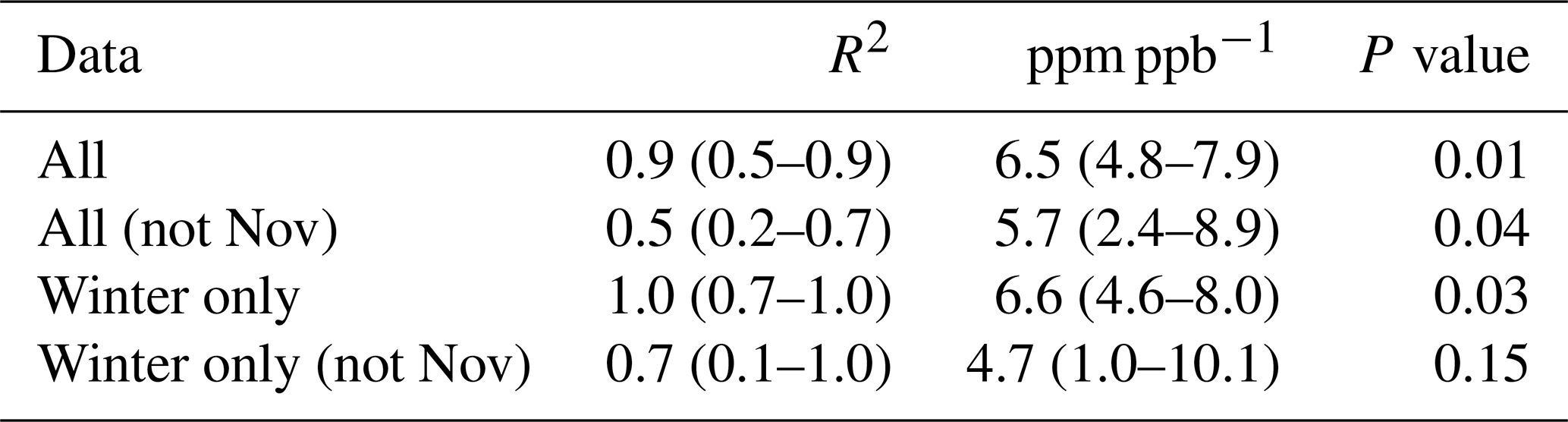
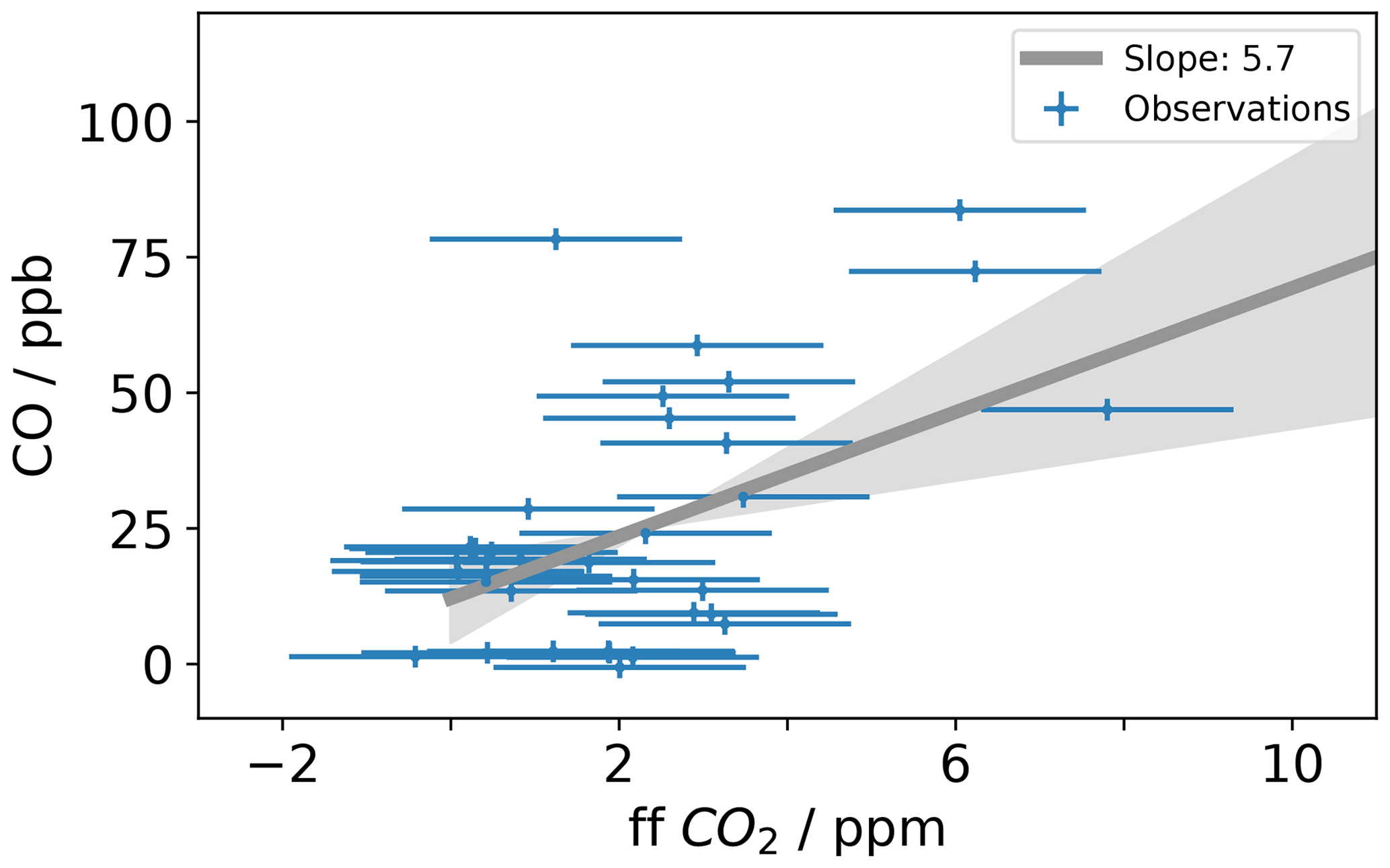
Figure 5 This figure shows the CO enhancement (CO_enh) at TAC (Sect. 4.2.3) against the observed ffCO₂ derived from Δ¹⁴CO₂ measurements. The slope of the linear regression is used to calculate the CO_enh∕ffCO₂ ratio at TAC. The grey line shows the linear regression and grey shading shows the 5 %–95 % uncertainty estimate of the linear regression. Results of the linear regression calculation of different subsets of this dataset can be found in Table 2.

5 Discussion

This work evaluated the use of Δ¹⁴CO₂ observations to derive the amount of CO₂ from fossil fuel burning that was recently added to the atmosphere in the UK. It was suspected that the relatively high density of ¹⁴CO₂ emitting nuclear sites could mask any Δ¹⁴CO₂ depletion caused by emissions from fossil fuel burning. It was found that while ¹⁴CO₂ emissions from nuclear industry sites in the UK do have an impact on Δ¹⁴CO₂ observations at TAC, this influence is not prohibitive of utilizing Δ¹⁴CO₂ observations for the determination of ffCO₂. However, the generally large uncertainties associated with Δ¹⁴CO₂ observations mean that, at TAC, the observed depletion in Δ¹⁴CO₂ due to a ffCO₂ signal is often below the detection limit (Δ¹⁴CO₂ depletion <5 ‰ in about 50 % of the flask samples). Other countries or locations without a large enough ffCO₂ signal to get a significant Δ¹⁴CO₂ depletion can use sampling techniques that integrate the ffCO₂ signal over weeks or months to increase the signal strength. In the UK, however, this would not be easily applicable as both the ¹²CO₂ from fossil fuel burning and the ¹⁴CO₂ from nuclear sites would be integrated. The correction for ¹⁴CO₂ emissions from nuclear industry sites would be difficult to apply as long temporal integration of the sample would increase the chances of a routine blowdown or a maintenance event (with high ¹⁴CO₂ emissions) occurring at a nuclear reactor nearby.

Generally, the radiocarbon method of determining the ffCO₂ enhancement would perform better if stronger signals were encountered more frequently. To find sampling locations in the UK that would be suitable to use for determining ffCO₂ with the radiocarbon method, a NAME forward model was used. A 1-year forward run was performed in NAME for both CO and ¹⁴CO₂ (June 2012–June 2013). CO was used as a proxy for fossil fuel CO₂ instead of the EDGAR 2010 emissions as there was a CO emission file correctly formatted for the use in NAME available to the authors. To convert the simulated CO values to ffCO₂, the CO_enh∕ffCO₂ ratio of 5.7 ppb ppm⁻¹, determined in Sect. 4.2.3, was used. These two simulations are then combined, dividing the average yearly increase in the Δ¹⁴CO₂ due to nuclear emissions (Δ¹⁴CO_2 nuclear) by the average yearly decrease in the Δ¹⁴CO₂ signal due to emissions from fossil fuel burning (ΔCO_2 ff). This ratio, illustrated in Fig. 6, indicates areas of the UK that would provide suitable sampling locations. A ratio lower than 1 indicates that, on average, the depletion due to fossil fuel burning is lower than the enhancement due to nuclear emissions and as such is a better location for radiocarbon measurements. A ratio of 1 indicates that, on average, the depletion expected due to fossil fuel burning at a location is equal to the enhancement due to emission from ¹⁴CO₂ from nuclear sites. It is important to recognize that this ratio is obtained by dividing simulated yearly averages, and it therefore shows the locations that are on average favourable for Δ¹⁴CO₂ sampling. Locations that have a high ratio, are less likely to be suitable for Δ¹⁴CO₂ sampling, either because they are heavily influenced by ¹⁴CO₂ emissions from nuclear industry sites or because the site is unlikely to be exposed to large fossil fuel emissions. This work also aimed to evaluate if ffCO₂ derived from Δ¹⁴CO₂ observations could be used in inverse models to preform top-down emission estimates. This work shows that although ffCO₂ derived with the radiocarbon method can be used to investigate national emissions, the relatively low depletion in Δ¹⁴CO₂ (due to CO_2 ff) in well-mixed air masses over the UK mean that applying the method to city scale emissions, where emissions are closer and therefore less diluted, might be more suitable. Figure 6 shows that sampling stations located closer to a region with higher emissions such as Greater London are more likely to encounter ffCO₂ enhancements that would lead to significant and therefore measurable depletions in Δ¹⁴CO₂; this would optimize the scientific value of the cost-intensive Δ¹⁴CO₂ measurements. In addition, improving the precision of the correction terms applied to the ffCO₂ calculations is also important. This could be achieved through the provision of higher-frequency nuclear industry emission data for ¹⁴CO₂ in the UK, improvements in the biospheric correction, and a reduction in the measurement uncertainties associated with Δ¹⁴CO₂ observations. This would improve the usability of the radiocarbon method in the UK.

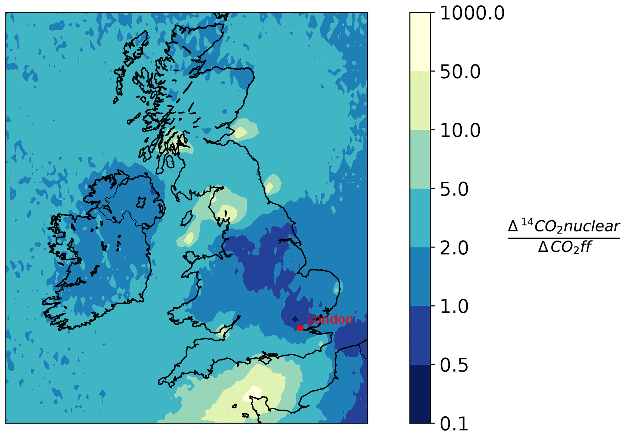
Figure 6 This figure shows the ratio of modelled ¹⁴CO₂ nuclear values (¹⁴CO₂ nuclear) to modelled fossil fuel CO₂ values (CO₂ff) in the UK and Ireland. The values represent yearly averages, calculated with a 1-year (June 2012–June 2013) forward run performed in NAME. CO was used as a proxy for ffCO₂ and the conversion factor (5.7 ppb ppm⁻¹) was used to convert CO to CO₂ (see Sect. 5). High values in yellow represent regions with a large influence from nuclear ¹⁴CO₂ emissions compared to the fossil fuel emissions, whereas darker blue areas with a lower ¹⁴CO₂∕ffCO₂ ratio represent areas where the influence from fossil fuel emissions on Δ¹⁴CO₂ is larger than the influence from nuclear emissions.

6 Conclusions

This study has provided valuable insights into the viability of using Δ¹⁴CO₂ measurements in the UK to determine recently emitted CO₂ from fossil fuel. It was shown that the UK fossil fuel emissions estimates from EDGAR are consistent with the observations. Despite the comparatively high density of ¹⁴CO₂-emitting nuclear reactors, corrections applied for nuclear emissions are not generally larger than those applied to account for the biospheric disequilibrium. However, both corrections add to the uncertainty in observed ffCO₂ values. The largest issue with using ¹⁴CO₂ observations at TAC for national emission estimates is that the measurement uncertainty is often higher than the observed and predicted depletion in radiocarbon. The derived ffCO₂:CO ratio is consistent with the inventory (NAEI 2014). However, uncertainties are large and use of a simple ratio may not account for all of the variability. The use of radiocarbon to estimate UK emissions could be improved in various ways. Higher-frequency automated sampling, allowing sampling at optimal time periods, would be one way to address this; another way would be to select optimal sampling locations as illustrated in Fig. 6. Prior to ¹⁴CO₂ analysis, assessment of the back trajectories and analysis of mole fraction trace compounds could be performed to ensure samples are collected during ideal conditions.