the Creative Commons Attribution 4.0 License.
the Creative Commons Attribution 4.0 License.
 | 20 Nov 2019
Potential regional air quality impacts of cannabis cultivation facilities in Denver, Colorado
Chi-Tsan Wang
Christine Wiedinmyer
Kirsti Ashworth
Peter C. Harley
John Ortega
Quazi Z. Rasool
William Vizuete
The legal commercialization of cannabis for recreational and medical use has effectively created a new and almost unregulated cultivation industry. In 2018, within the Denver County limits, there were more than 600 registered cannabis cultivation facilities (CCFs) for recreational and medical use, mostly housed in commercial warehouses. Measurements have found concentrations of highly reactive terpenes from the headspace above cannabis plants that, when released in the atmosphere, could impact air quality. Here we developed the first emission inventory for cannabis emissions of terpenes. The range of possible emissions from these facilities was 66–657 t yr−1 of terpenes across the state of Colorado; half of the emissions are from Denver County. Our estimates are based on the best available information and highlight the critical data gaps needed to reduce uncertainties. These realizations of inventories were then used with a regulatory air quality model, developed by the state of Colorado to predict regional ozone impacts. It was found that most of the predicted changes occur in the vicinity of CCFs concentrated in Denver. An increase of 362 t yr−1 in terpene emissions in Denver County resulted in increases of up to 0.34 ppb in hourly ozone concentrations during the morning and 0.67 ppb at night. Model predictions indicate that in Denver County every 1000 t yr−1 increase in terpenes results in 1 ppb increase in daytime hourly ozone concentrations and a maximum daily 8 h average (MDA8) increase of 0.3 ppb. The emission inventories developed here are highly uncertain, but highlight the need for more detailed cannabis and CCF data to fully understand the possible impacts of this new industry on regional air quality.
- Article
(5261 KB) - Full-text XML
-
Supplement
(1776 KB) - BibTeX
- EndNote


The rapid expansion of one of the United States' newest industries, the commercial production and sale of recreational cannabis, was recently likened to the millennial “dot-com” boom (Borchardt, 2017). With an increasing number of states passing bills to legalize recreational cannabis, the enterprise is set to rival all but the largest of current businesses. The cultivation, sale, and consumption of recreational cannabis annual sales revenues had reached USD 1.5 billion in the US state of Colorado by 2017 (CDOR, 2018b), exceeding revenues generated by grain farming in the state. The commercial cultivation and sale of cannabis is not subject to the same strict environmental monitoring and reporting procedures as other industries of similar size. While the relaxation of laws has provided certain medicinal and economic opportunities for the states involved, the potentially significant environmental impact on air quality due to the production of cannabis has largely been ignored.
Previous research on the wider impacts of cannabis production has been limited due to its federal status as an illegal or controlled substance (Crick et al., 2013; Eisenstein, 2015; Andreae et al., 2016; Stith and Vigil, 2016). As a result of this status, most studies have focused on the pharmacological and health effects of the psychoactive constituents of Cannabis spp. (Ashton, 2001; Borgelt et al., 2013; WHO, 2016), or the societal impacts associated with the illicit nature of the industry (IDCP, 1995; Sznitman and Zolotov, 2015; WHO, 2016). The few assessments to date on the environmental impacts of the production of Cannabis spp. have centered on the detrimental effects of outdoor cultivation on ecosystems and watersheds due to land clearance and high water demand (Bauer et al., 2015; Carah et al., 2015; Butsic and Brenner, 2016). Studies have also quantified the energy consumption of the industry and the resulting greenhouse gas emissions associated with indoor cultivation (Mills, 2012). Little attention has been paid to the possible biogenic volatile organic compounds (BVOCs) emitted from the growing of cannabis and its impact on indoor and outdoor air quality.
The only studies that have measured the composition of gaseous emissions from cannabis have been limited to headspace samples above the plants (Hood et al., 1973; Turner et al., 1980; Martyny et al., 2013). These studies have shown high concentrations of VOCs such as monoterpenes (C10H16), sesquiterpenes (C15H24), and cannabinoids. These studies also measured thiols, a sulfur-containing compound responsible for the characteristic odor of Cannabis spp. (Rice and Koziel, 2015a, b). The principle (trace) components are reported to be α- and β-pinene, β-myrcene, d-limonene, cis-ocimene, β-caryophyllene, β-farnesene, and α-humulene (Hood et al., 1973; Turner et al., 1980; Hillig, 2004; Fischedick et al., 2010; Martyny et al., 2013; Marchini et al., 2014; Rice and Koziel, 2015a). The precise mix of chemical species, however, was strongly dependent on strain and the growing conditions (Fischedick et al., 2010). It should be noted that the pharmacologically active ingredients, e.g., tetrahydrocannabinol (Δ9-THC), generally have low-volatility and therefore are rarely detected in the gas phase (Martyny et al., 2013). Measurements in (illicit) cannabis cultivation facilities (CCFs) in conjunction with law enforcement raids in Colorado in 2012 found VOC concentrations of terpenes to be 50–100 ppb within growing rooms (Martyny et al., 2013). In these cases, the CCF operation contained fewer than 100 plants, compared with the thousands of plants found in currently licensed premises (CDOR, 2018a). Further, the Spokane Regional Clean Air Agency (SRCAA) study in Washington state measured indoor VOCs in seven flowering rooms and two dry bud rooms across four different CCFs. The average terpene concentration was 361 ppb (27–1676 ppb) in those facilities (Southwellb et al., 2017). These indoor measurements indicate the presence of BVOCs, but only limited studies have actually determined the chemical profile of gases actually emitted by the growing plants. For comparison, summertime outdoor monoterpene concentrations in forested regions of Colorado are typically less than 4 ppb (Ortega et al., 2014).
Terpenoids, such as monoterpenes (C10H16) and sesquiterpenes (C15H24), are highly reactive compounds with atmospheric lifetimes ranging from seconds to hours (Fuentes et al., 2000; Seinfeld and Pandis, 2006). They are primarily biogenic in origin (Fuentes et al., 2000; Guenther et al., 2012) and their reactions alter the atmospheric oxidizing capacity, resulting in a range of low volatility products that can partition into the aerosol phase and, depending on the concentration of nitrogen oxides (NOx), lead to the formation of ozone (Laothawornkitkul et al., 2009; Guenther et al., 2012). Both ozone and aerosols are climate-relevant components of the atmosphere as well as critical air pollutants (USEPA, 2016).
In Colorado, the commercial growing of Cannabis spp. is restricted to secure and locked premises, resulting in indoor operations in most counties (CDOR, 2018a). Since legalization, the number of cannabis cultivation facilities (CCFs) has risen to 1400 across the state of Colorado in 2018, including more than 233 registered recreational and 375 medical CCFs within the Denver city limits alone. In Denver, the CCFs are commonly housed in commercial warehouses and the majority of these are located near transport links such as train hubs and major interstate highways (CDOR, 2019; Mills, 2012). Denver and the Front Range area are currently classified as “moderate” non-attainment of the ozone standard (USEPA, 2017). Due to that status, a federally mandated State Implementation Plan (SIP) was developed and mutually agreed upon between the state of Colorado and the United States Environmental Protection Agency (EPA) (CDPHE, 2009). Under the terms of the SIP, Colorado Air Quality Control Commission (AQCC) developed regulatory models to predict reductions in ozone precursors (CDPHE, 2009). These studies have found that ozone concentrations in Denver are VOC-sensitive, meaning that an increase in VOC concentrations will increase ozone production (UNC-IE and ENVIRON, 2013). The location of CCFs in a VOC sensitive region in Denver suggests a potential emission source that may impact regional air quality (UNC-IE and ENVIRON, 2014). This work used the best available information to produce the first emission inventory of VOCs from CCFs in Colorado. Colorado's regulatory model was then used to determine the extent that these emissions could impact regional air quality.
2.1 Emission rate calculation
Figure 1a shows the locations of the licensed 739 recreational and 733 medical CCFs in Colorado as of March 2018 (CDOR, 2018a). Equation (1) was first used to estimate an emission rate for each CCF, and then all CCFs were used to build a bottom-up BVOC emission inventory.
where ERi (µg h−1) is the total emission rate for CCF i based on the sum of emission rates for all j cannabis strains; ECij is the emission capacity (; dwg is dry weight in grams) for cannabis strain j in facility i, DPWij is the dry plant weight in grams per plant for cannabis strain j, and PC is the plant count number for strain j in facility i.

Figure 1(a) The locations of medical (red) and retail (green) Cannabis cultivation facilities (CCFs) in Colorado as of 1 March 2018. The corresponding values are the number of CCFs found within each city. The base map layer of this figure was made by Esri (Esri et al., 2013). (b) The 36 km ×36 km resolution of Western Air Quality Study (WAQS) and nested inner 12 km ×12 km resolution domains and 4 km ×4 km resolution domain used by the Comprehensive Air Quality Model with extensions (CAMx). This map was made by ENVIRON and Alpine Geophysics (ENVIRON and Alpine Geophysics, LLC, 2017b).
Since state legalization only occurred in 2014, and given the current federal illicit status of Cannabis spp., there is a lack of available data for the three parameters used in Eq. (1). The following describes the assumptions made for a range of potential values of EC, DPW, and PC given the best information available.
2.1.1 Emission capacity (EC)
The only data of EC from a leaf enclosure measurement are of three strains, namely Critical Mass, Lemon Wheel, and Rockstar Kush, that were 45 d old (Wang et al., 2019). This study found that at this growth stage the EC for total monoterpenes varied among strains: 10 for Critical Mass, 7 for Lemon Wheel, and 6 for Rockstar Kush. The Department of Revenue (DOR) in Colorado has classified Cannabis spp. in a CCF into four different growth stages: immature (0–24 d old), vegetative (25–79 d old), flowering (80–132 d old), and at harvest (132–140 d old) (Hartman et al., 2018a). Wang et al. (2019) only sampled during the vegetative stage, and to our knowledge emission rates of monoterpenes from buds or flowers do not exist. It is not known how much EC will change during these different growth stages, but the grey literature does report that CCFs actively select cultivars to maximize the amount of monoterpenes found in the bud tissues.
The Spokane Regional Clean Air Agency (SRCAA), in collaboration with Washington State University (Southwellb et al., 2017; Wen et al., 2017), measured monoterpenes in flowering rooms of CCFs in Washington State. They found concentrations of monoterpenes in the growing room with 80 d old plants (1660 ppb) to be >10 times higher than the 48 d old plants (150 ppb). CCFs in Colorado house a wide variety of strains at both vegetative and flowering stages of growth, suggesting that the emission rate of monoterpenes from CCFs is higher than that measured from foliage by Wang et al. (2019). Currently, no database exists that can provide the number of plants by strain and growth stage. For the base case, it was assumed that each CCF grew only one strain and that all plants were at the vegetative growth stage, resulting in a single and constant EC for each CCF, taken to be 10 of total monoterpenes based on the reported EC from the Critical Mass cultivar (Wang et al., 2019). Given the uncertainty in EC and the variety of possible plant stages and cultivars, the EC used in simulation 1_EC was multiplied by a factor of 5 and 10 in simulations 2_EC and 3_EC as a sensitivity analysis.
2.1.2 Dry plant weight (DPW)
No published studies report the DPW of a Cannabis spp. plant. Both the states of Colorado (METRC, 2018) and Washington (LCB, 2017; Topshelfdata, 2017) track the mass of the commercially sold portion of the plant, the “dry bud”. The Colorado database, however, is not publicly accessible and was not available for this study. In Washington, using data from all types of facilities (outdoor and indoor) from August to October 2017, it was found that the average dry bud mass per plant was 210 g (0–586 g) shown in Fig. S1a in the Supplement. The Washington database also includes the “wet bud” weight defined as the mass of the bud after it was just harvested (Fig. S1b in the Supplement), but prior to the 7–10 d drying process. The total waste weight, or the remaining mass of the plant after the buds have been harvested, is also recorded. As shown in Eq. (2), the sum of these two masses should equal the total mass of the wet plant.
where Mwet plant is the mass of the entire wet plant (g), Mwet bud is the mass of the wet bud (g), and Mwet waste is the mass of the waste (g).
Data from August to October 2017 were used with Eq. (2) to estimate the wet plant weight resulting in an average of 3770 g (6–13 405 g) shown in Fig. S1c. The large range in mass is due to the different growing conditions found in CCFs, and the type of strain being grown. The ratio of the wet and dry bud mass data from Washington was used as a surrogate to determine the percentage of water found in the total plant material as shown in Eq. (3).
where RD∕W is the ratio of the masses of the dry to wet bud, and Mdry bud (g) is the mass of the harvested buds after 7–10 d of drying (Fig. S1d).
It was assumed that the same factor could be applied to the total wet plant weight to estimate the DPW as shown in Eq. (4).
The average of DPW was 754 g (1–2260 g). For the development of these emission inventories, a base value of 750 g was assumed for DPW based on the average calculated from the Washington database. As a sensitivity test, a DPW of 1500 g representing the mean plus 1 standard deviation range was chosen. Finally, a DPW of 2500 g, the maximum yield recorded by Washington State Liquor and Cannabis Board, was taken as the upper statistical boundary as shown in Fig. S1e. As the total plant count and reported yields are a factor of 3 and 4 higher, respectively, in Colorado than Washington State (LCB, 2017; Topshelfdata, 2017; Hartman et al., 2018a), we took this maximum on the assumption that Cannabis spp. cultivated in CCFs in Colorado in the summer season are grown under more optimal conditions than those grown in Washington State, resulting in considerably higher yields.
2.1.3 Plant count (PC)
Counts of all plants larger than 20.3 cm have been recorded by the Colorado DOR on a monthly basis since 2014. As of June 2018, there are a total of 1.06 million plants (Hartman et al., 2018a, b). We therefore used 1 million as the base number for the emission inventory. The DOR data only provide county-level information rather than actual number of plants per CCF. The plants were then distributed equally among the CCFs to calculate an average of 905 plants per facility in Denver County and 521 outside of the county.
Two sensitivity simulations were conducted based on the assumption that the cannabis industry in Colorado will continue to expand at similar rates in the future. From June 2016 to June 2018 the total number of plants recorded by DOR grew from 826 963 to 1 062 765, an annual average increase of 118 000. Assuming this rate of expansion remains constant, there would be 2 million plants in the state of Colorado by 2025 and this value was used in simulation 6_PC. It was assumed in simulation 7_PC that growth would accelerate in the future to the point at which each recreational and medical CCF would contain the maximum number of plants permitted under a Tier 1 license leading to a statewide total of nearly 4 million plants. The maximum number of plants that can be grown under each licensing tier is shown in Table S2 in the Supplement (CDOR, 2019). The average plant count per CCF for each PC sensitivity simulation is shown in Table S1.
2.2 Emission inventories for cannabis cultivation facilities (CCFs)
Given the large gaps in knowledge, this study will focus only on variabilities in EC, DPW, and PC and will hold other parameters constant. For example, to maximize growing conditions relative humidity, temperatures, CO2 concentrations, and fertilizer usage are all optimized and vary widely by CCF. Further, this study did not consider other processes such as trimming, harvesting, and drying buds, which may also release BVOCs.
For this study, it was assumed that all CCFs operated in the same way at a temperature of 30 ∘C and 1000 of photosynthetically active radiation (PAR). In addition, it was assumed that all emissions from the plants inside a CCF enter the atmosphere. Ventilation to the atmosphere varies widely by the operation, and there are no current regulations or industry-wide practices that are being used to mitigate emissions.
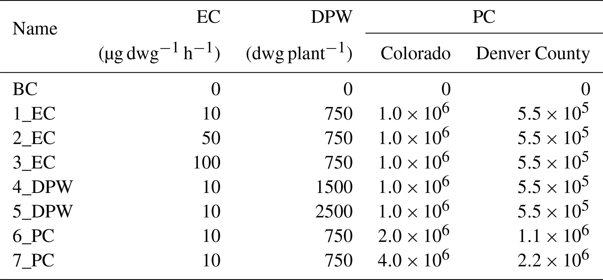
In total, seven scenarios of emission inventories were created to explore sensitivities in EC, DPW, and PC as shown in Table 1. In scenarios 1–3, the PC was held to a total of 1 million and a 750 g DPW was assumed. The EC of 10 as reported by Wang et al. (2019) was used in 1_EC, with a sensitivity that multiplied that rate by a factor of 5 (scenario 2_EC) and 10 (scenario 3_EC). The remaining scenarios in Table 1 kept the EC constant at 10 . Scenarios 4_DPW and 5_DPW explored the sensitivity of increasing DPW, and scenarios 6_PC and 7_PC increased the total plant count.
Table 1Simulation scenarios and assumed values for emission capacity (EC) rate, dry plant weight (DPW), and the plant count (PC) for Colorado and Denver County. The base case (BC) scenario has no cannabis emissions.
2.3 Model description and analysis tools
2.3.1 Model protocols and evaluation
The Comprehensive Air Quality Model with Extensions, CAMx6.10 (ENVIRON, 2013; ENVIRON and Alpine Geophysics, LLC, 2017b), was used to predict ground-level ozone concentrations. The model and protocols used in this study are based on the Western Air Quality Study (WAQS) for 2011 (ENVIRON and Alpine Geophysics, LLC, 2017b; Adelman et al., 2016). The WAQS 2011b baseline model simulation period runs from 15 June to 15 September 2011, and is driven with meteorological data from WRF version 3.3 for the same time period and domain. The model was initialized using Three-State Air Quality Modeling Study standard boundary and initial conditions (ENVIRON and Alpine Geophysics, LLC, 2017b). The model domain is a two-way nested grid at 12 and 4 km grid cell resolutions (Fig. 1b). Anthropogenic emissions were derived from EPA National Emission Inventory (NEI) version 2011 NEIv2 with updates for point and area sources of oil and gas emissions in the western US. The biogenic emission inventory was based on the Model of Emissions of Gases and Aerosols from Nature version 2.1 (MEGANv2.1) (Guenther et al., 2012). All data and supporting documentation are publicly available via the Intermountain West Data Warehouse (IWDW) website (WAQS, 2017).
The revision 2 of the Carbon Bond 6 (CB6r2) (Ruiz and Yarwood, 2013) chemistry mechanism was used in all model runs. This groups all monoterpenes as a single compound species, TERP. Thus, the total monoterpene EC reported in Wang et al. (2019) was converted into the TERP species. TERP undergoes oxidation reactions with the nitrate radical (NO3), the hydroxyl radical (OH), ozone (O3), and singlet oxygen. It should be noted that the TERP category includes a wide variety of monoterpenes whose reaction rate constants may differ from TERP ( molecules cm−3 s−1). For example, the rate constant of β-myrcene with OH radical (Hites and Turner, 2009) is molecules cm−3 s−1 (k298), which is 4 times higher than TERP and 5.6 times faster than α-pinene (Carter, 2010).
The details of the WAQS model setup protocol (ENVIRON and Alpine Geophysics, LLC, 2017b) and model performance (Adelman et al., 2016) can be found on the IWDW website. In summary, the model performance evaluation concluded that this simulation had met all performance goals for both maximum daily 1 h (MDA1) and maximum daily 8 h average (MDA8) ozone. In the performance review report, it was found that the WAQS model had a positive bias for ozone simulated in a 4 km ×4 km resolution domain, when compared with EPA Air Quality System (AQS) surface monitors (MDA1: 0.8 %, MDA8: 0.9 %). On days when ozone concentrations higher than 60 ppb were measured, the model had a negative bias of −6.2 % for MDA1 and −6.3 % for MDA8. The model evaluation result also noted that the model performance was best during the spring and summer months.
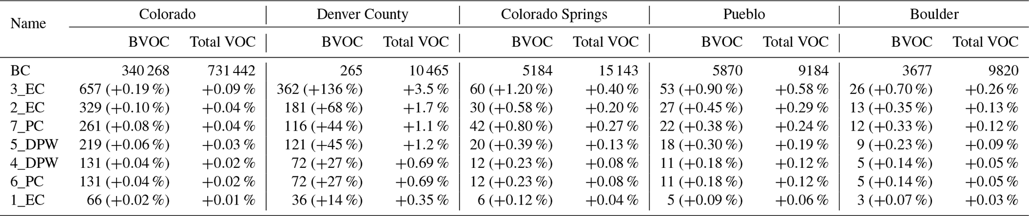
Table 2The estimated BVOC and total VOC emission rates (t yr−1) for the base case (BC) scenario. Also shown are the increases in VOC emissions for all scenarios shown in Table 1 for Colorado, Denver County, Colorado Springs, Pueblo, and Boulder. The numbers in parentheses are the percentage increases compared with the BC scenario.
2.3.2 Process analysis
CAMx runs used in this analysis had the process analysis (PA) option enabled (ENVIRON, 2013). The CAMx configuration used here produces two additional files needed for PA: the integrated reaction rate (IRR) and integrated process rate (IPR). These files include the rates of change in concentration of every species due to chemistry and transport for every grid cell and time step. Python-based Process Analysis (pyPA) and the Python Environment for Reaction Mechanisms/Mathematics (PERMM) (Henderson et al., 2010, 2011) were then applied to post-processing the CAMx PA output. PERMM was used to aggregate the chemical and physical process rates for selected model grid cells and layers, allowing for tracking of plumes within the planetary boundary layer (PBL).
3.1 Emission inventory
The seven scenarios were used to estimate a range of emissions of BVOCs from CCFs for the entire state of Colorado. As shown in Table 2, the base case (BC) scenario estimates 731 442 t yr−1 of all VOCs being emitted in Colorado, of which 47 % are BVOCs. The BC scenario does not include any emissions from the cannabis industry. Table 2 also shows the seven scenarios that did include CCF emissions ranked in order of their increases in statewide BVOC emissions. As expected the CCF BVOC emissions scaled linearly with each factor that was changed in Eq. (1). In scenario 3_EC, a 10-fold increase in the emission rate (100 ) resulted in a 657 t yr−1 increase. Similarly, scenario 2_EC assumes 50 and produces 329 t yr−1. Scenarios 4 and 5 showed the sensitivity of terpene emissions from CCFs to variation in DPW while holding PC constant and an EC of 10 . It was estimated that an additional 66 t yr−1 of emissions is produced when a 750 g DPW is assumed. This doubles to 131 t yr−1 with a DPW of 1500 g and reaches 219 t yr−1 with a DPW of 2500 g. Comparing scenario 1_EC with scenarios 6 and 7 shows how the growth in PC will impact emissions of BVOCs. In Colorado, a doubling of the PC increases BVOC emissions by 131 t yr−1 in scenario 6_PC and 261 t yr−1 for the 4 million plants in scenario 7_PC. The largest increases in BVOC emissions were predicted in scenarios 3_EC and 2_EC showing that the total emission rate of BVOCs from CCFs was most sensitive to EC.
In March 2018, Denver County housed 41 % of CCFs and 55 % of all cannabis plants in Colorado (Hartman et al., 2018b). As a result, about 43 % of statewide CCF BVOC emissions occur there (Table 2). Current emission inventories of Denver County show negligible amounts of biogenic emissions accounting for only 0.1 % of the total statewide BVOC emissions. CCF emissions increased BVOC emission rates in Denver Country up to 136 % in scenario 3_EC. This changes the total VOC emission rate in Denver County by up to 3.5 %. Other cities in Colorado do not have as high of a concentration of CCFs, and thus the relative increases were smaller as shown in Table 2.
The introduction of additional cannabis BVOC emissions into model simulations increased the predicted TERP concentrations. Figure 2 shows the maximum increase in TERP concentrations for three scenarios for Denver County over the entire 90 d simulation period. Regardless of the scenario, the largest increases in TERP occurred near the largest concentrations of CCFs. The absolute maximum changes ranged from 0.5 to 5.0 ppb located at the Elyria–Swansea and Globeville neighborhoods in north-central Denver. Increases in TERP were also predicted to the north due to the dominant wind flows in that direction throughout the simulation period. Figure S2 shows the maximum increase in TERP concentrations for the 1_EC, 5_DPW, and 3_EC scenarios in the 4 km ×4 km domain for the entire 90 d simulation period. As expected substantially lower increases in TERP concentrations were predicted for other cities in Colorado: 0.26 ppb in Colorado Springs and 0.24 ppb in Pueblo. Figure 3 shows the hourly changes in TERP concentrations across the entire 4 km ×4 km domain. The largest increases for all scenarios occurred at night with a peak of 5 ppb at 04:00 local standard time (LST). Given that the hourly emissions of terpenes from CCFs were assumed constant for 24 h, these larger nighttime changes can be primarily ascribed to the lack of photochemistry and a shallow nocturnal PBL. These results suggest that the increases in TERP are highly correlated with locations of CCFs, accumulate at night, and have significant losses during the day.
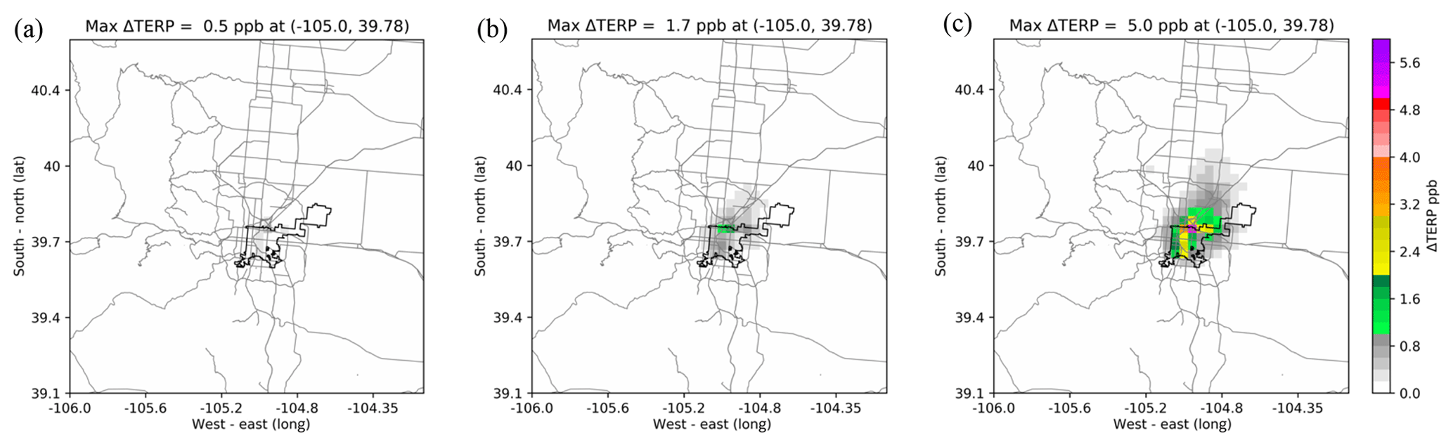
Figure 2The maximum increase in TERP concentrations (ppb) for Denver County and Front Range over the entire 90 d simulation for the (a) 1_EC, (b) 5_DPW, and (c) 3_EC scenarios. The black outlines Denver County and the grey lines are state and interstate highways.
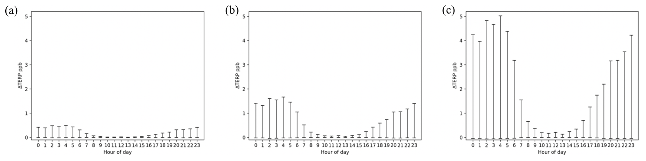
Figure 3The hourly changes in TERP concentrations across the entire 4 km ×4 km domain, over the 90 d simulation for the (a) 1_EC, (b) 5_DPW, and (c) 3_EC scenarios.
3.2 Regional ozone impacts
Predicted increases in hourly ozone concentrations in excess of 0.1 ppb only occurred when terpene emissions were in excess of 219 t yr−1, with scenarios 4_DPW, 6_PC, and 1_EC having little impact on predicted ozone. Thus, this analysis will focus on two scenarios, 5_DPW and 3_EC, to explore potential regional ozone impacts in the present and future. Figure 4 shows the hourly changes in ozone concentrations across the entire 4 km ×4 km domain for these two scenarios. During the daytime, the increase in TERP emissions results in a peak ozone increase of 0.34 ppb at 09:00 LST for 3_EC with only minimal changes in 5_DPW. Figure 5 shows, for Denver County and the Front Range metropolitan area, the locations of the daytime (06:00–18:00 LST) maximum increases in hourly ozone concentrations for all 90 d when emissions were added for scenarios 5_DPW and 3_EC. Ozone increases for the entire 4 km ×4 km domain can be found in Fig. S3. The largest predicted ozone concentrations occurred in Denver County with impacts of 0.11 ppb in 5_DPW and 0.34 ppb in 3_EC as shown in Fig. 5. Both scenarios show that daytime increases in ozone were limited to Denver County and just to the northwest, west, and southwest of Denver County.

Figure 4The predicted differences in hourly ozone concentrations (ppb) across the entire Colorado domain, over the 90 d simulation for the (a) 5_DPW and (b) 3_EC scenarios.
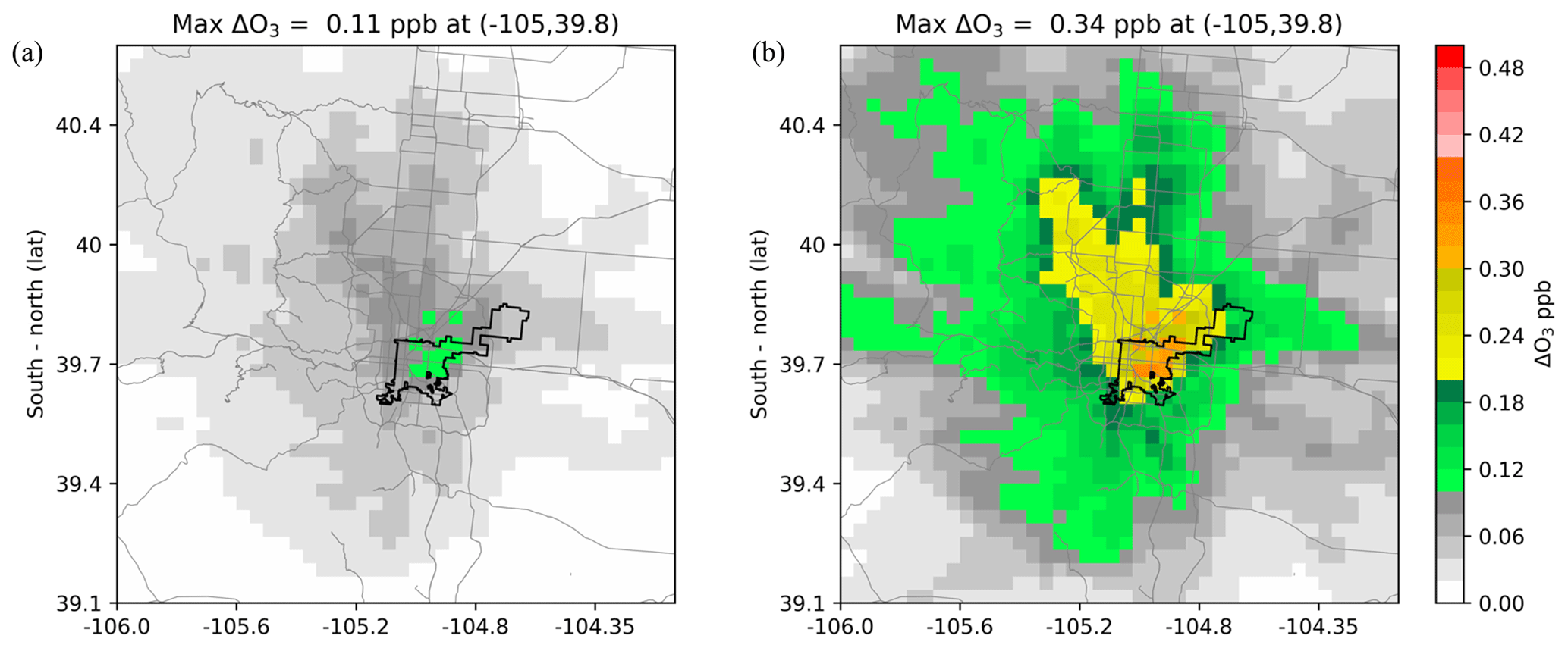
Figure 5The predicted changes in hourly ozone concentrations for the Denver region from 06:00 to 18:000 LST for all 90 d of the simulation for the (a) 5_DPW and (b) 3_EC scenarios. The grey lines indicate major highways and the black line outlines Denver County.
There were also nighttime variations in ozone observed for the modeling domain. In scenarios 5_DPW and 3_EC, nighttime increases were more than double the increases predicted during the day. The largest changes in hourly ozone concentrations of 0.67 ppb occurred at 00:00 LST (i.e., midnight) for 3_EC. Figure 6 shows the location and magnitude of the maximum changes in hourly ozone concentrations during the night (18:00–06:00 LST) in 5_DPW and 3_EC. The extent of ozone increases at night is primarily to the north of Denver indicating a northern outflow. The maximum increase in hourly ozone for the whole of Colorado is shown in Fig. S3, with visibly little changes at night in other cities. These model results suggest that the additional emissions of TERP have immediate impacts on local ozone production chemistry during both the day and night, but little wider impact.
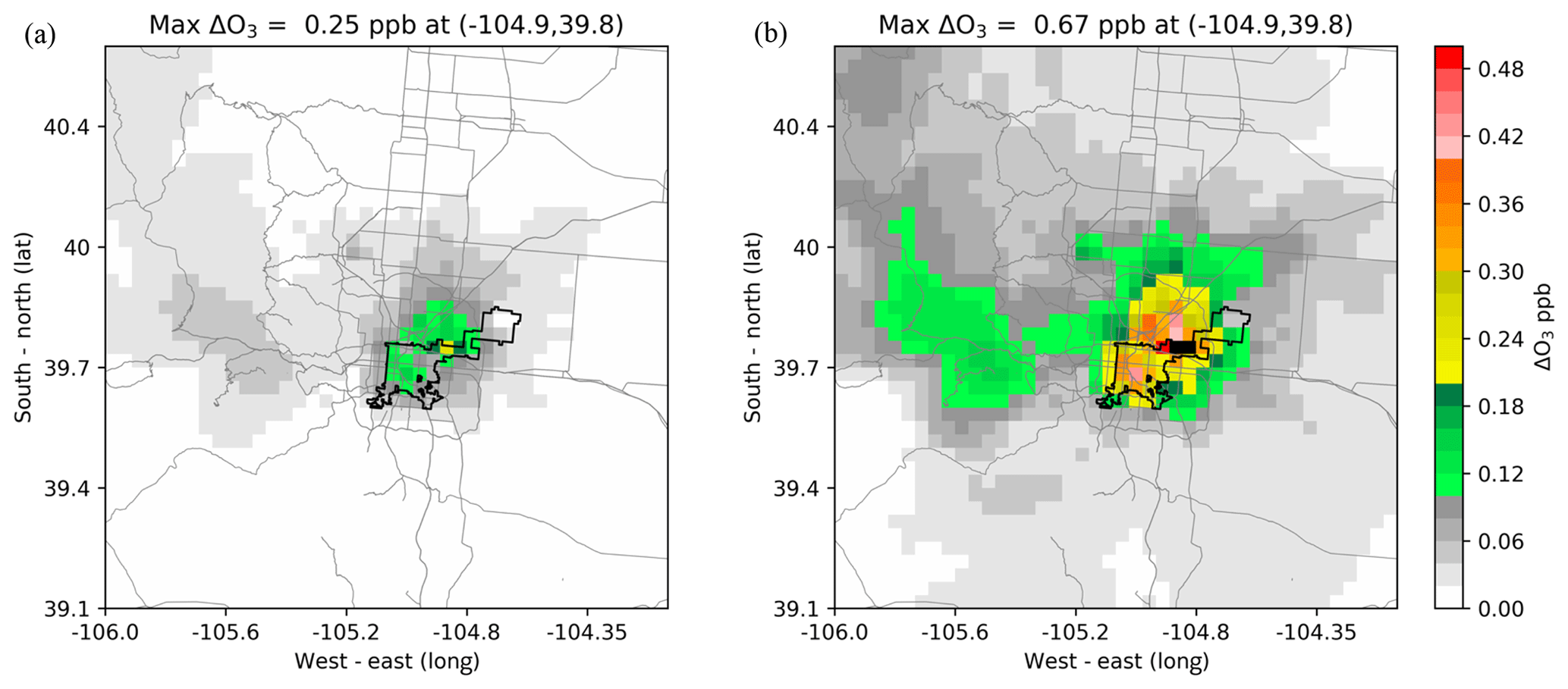
Figure 6The predicted changes in hourly ozone concentrations for the Denver region from 18:00 to 06:00 LST for all 90 d of the simulation for the (a) 5_DPW and (b) 3_EC scenarios. Black regions within the map indicate ozone increase values greater than 0.5 ppb. The grey lines indicate major highways and the black line outlines Denver County.
A critical metric for the attainment of the National Ambient Air Quality Standards (NAAQS) ozone standard in Denver County is the maximum daily average 8 h ozone concentration (MDA8). Figure 7 shows the maximum difference in MDA8 for each grid cell centered on Denver County, across the entire 90 d simulation period for the 5_DPW and 3_EC scenarios. Maximum increases in MDA8 are 0.14 ppb for 3_EC (Fig. 7b) co-located with the maximum increases in TERP concentrations.

Figure 7The predicted maximum increases in the maximum daily average 8 h (MDA8) ozone concentration (ppb) for the (a) 5_DPW and (b) 3_EC scenarios for the Denver region over the 90 d simulation period. The black indicates ozone increase values greater than 0.12 ppb.
3.2.1 Ozone impact at night
The maximum hourly ozone increase of 0.67 ppb for the 3_EC scenario occurred on Thursday, 28 July 2011, at 00:00 LST (i.e., midnight) near the largest concentration of CCFs (see Fig. 8). In subsequent hours the plume of ozone moved slowly to the east before being dispersed by the rise of the morning PBL at 06:00 LST.
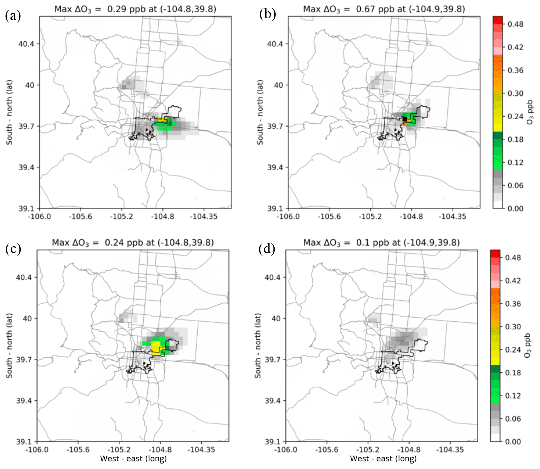
Figure 8For the 3_EC scenario on 28 July 2011, the largest hourly predicted ground-level ozone increases at (a) 27 July, 21:00 LST and for 28 July, at (b) 00:00 LST (i.e., midnight), (c) 03:00 LST, and (d) 06:00 LST.
To better understand why ozone increased at night, the PA model output was analyzed to quantify the chemical and physical processes producing ozone. Plume tracking was used so that only grid cells where the increase in ozone (i.e., the plume) occurred were included in our analysis, which ran from 27 July, 21:00 to 28 July, 06:00 LST. The number of vertical model layers included in the analysis also varied to incorporate the hourly evolution of the PBL. Figure S4 provides snapshots of the horizontal grid cells used and the vertical layers that were aggregated throughout the simulation time period. Figure S5 shows the changes in final ozone concentrations (compared to the base case) for the grid cells and vertical layers included in the analysis, as well as the physical and chemical process rates that account for these changes. Figure S5 shows that the process most responsible for increases in ozone concentrations was chemical production.
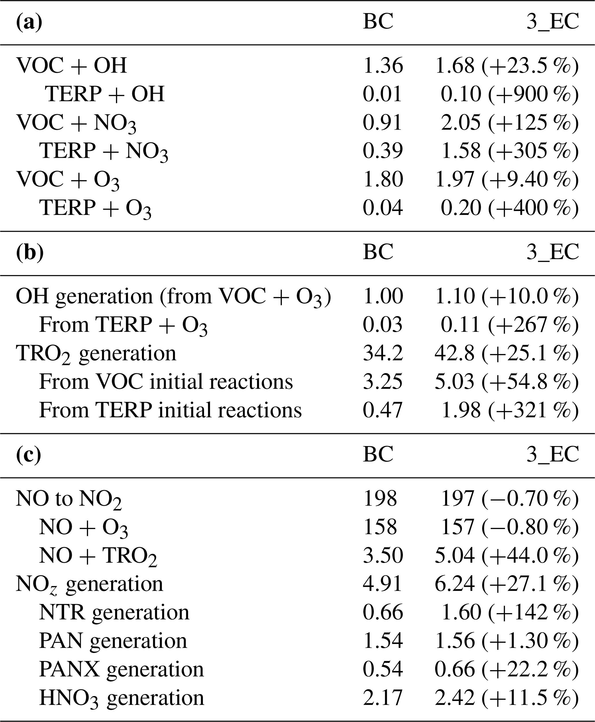
For the chosen vertical layers and grid cells Table 3a shows the total rate of the oxidation reactions with TERP across the entire period. Throughout this time, the additional TERP emissions lead to an increase in the number of oxidation reactions thereby generating more secondary VOC products and radical species. The chemical losses of TERP increased due to reactions with OH (from 0.01 to 0.1 ppb; +900 %), nitrate radical (NO3) (from 0.39 to 1.58 ppb; +305 %), and O3 (from 0.04 to 0.2 ppb; +400 %). Further analysis confirms that nighttime oxidation chemistry leading to changes in ozone concentration are driven by NO3. In the 3_EC scenario, TERP emissions only increased the annual VOC emission in Denver County by 3.5 %, but this is sufficient to increase the VOC + NO3 reaction rates by 125 %. These increases produce more peroxyl radicals (TRO2=HO2 + RO2) driving further oxidation and further radical production. Table 3b also shows that the generation of OH radicals from reactions of TERP with O3 increased by 267 %. Ultimately, these increases in initial TERP reactions with NO3 and O3 increase the NO-to-NO2 conversions via the TRO2 pathway by 44 %, reducing the availability of NO to react with O3. Thus, the increased ozone concentration predicted at night is actually due to the 1 ppb (0.8 %) reduction in the loss of ozone to reactions with NO rather than an increase in actual production of ozone (Table 3c). The increased TERP emissions also increase production of NOx termination products (NOz) by 27 % with organic nitrate (NTR; representing ∼71 % of this NOz product), increasing from 0.66 to 1.6 ppb (+142 %). This increase in NOz production at night also results in lower NO concentrations and thus lower ozone titration.
Table 3All data summed from 27 July, 21:00 LST to 28 July, 05:00 LST for grid cells and layers shown in Fig. S4. The base case (BC) scenario column shows the absolute predicted values and the subsequent columns show the predicted changes due to emissions from the 3_EC scenario. Percentages in parentheses are the changes in 3_EC relative to BC. Shown is the (a) total amount of VOC and TERP consumed due to oxidation (ppb), the (b) total amount of hydroxyl radical (OH) and total peroxyl radicals (TRO2) that were generated and their sources (ppb), and the (c) total amount of nitrogen dioxide (NO2) and NOx termination products (NOz) produced and their sources (ppb).
3.3 Ozone impact during the day
The maximum daytime hourly ozone increase of 0.34 ppb occurred at 09:00 on Monday, 18 July 2011, as shown in Fig. 9. On this day, the meteorological conditions favored the maximum possible production of ozone. This day featured “upslope flows” that are a common meteorological condition linked to ozone exceedance periods (Pfister et al., 2017). We thus chose to focus on 18 July to understand the daytime changes in chemistry that occur from increased BVOC emissions. As expected, the location of predicted ozone increases coincides with the location of the strongest terpene emissions in the domain as shown in Fig. 9a. For the daytime hours of 06:00–14:00 LST, the PA option was used to quantify changes in chemical processes for the grid cells and model layers shown in Fig. S6. For these grid cells and layers, Fig. S7 shows the changes in final ozone concentrations compared to the base case and the physical and chemical process rates that impact those concentrations. Table S3 sums the key chemical processes for these hours. The increases in CCF emissions resulted in a 100 % increase in OH reactions with TERP producing intermediate oxidation products and ultimately increasing OH production by 0.6 %. As a result of this oxidation chemistry, there was an increase of 0.9 % in NO-to-NO2 conversion by the TRO2 pathway, ultimately leading to a 0.1 % increase in ozone production.
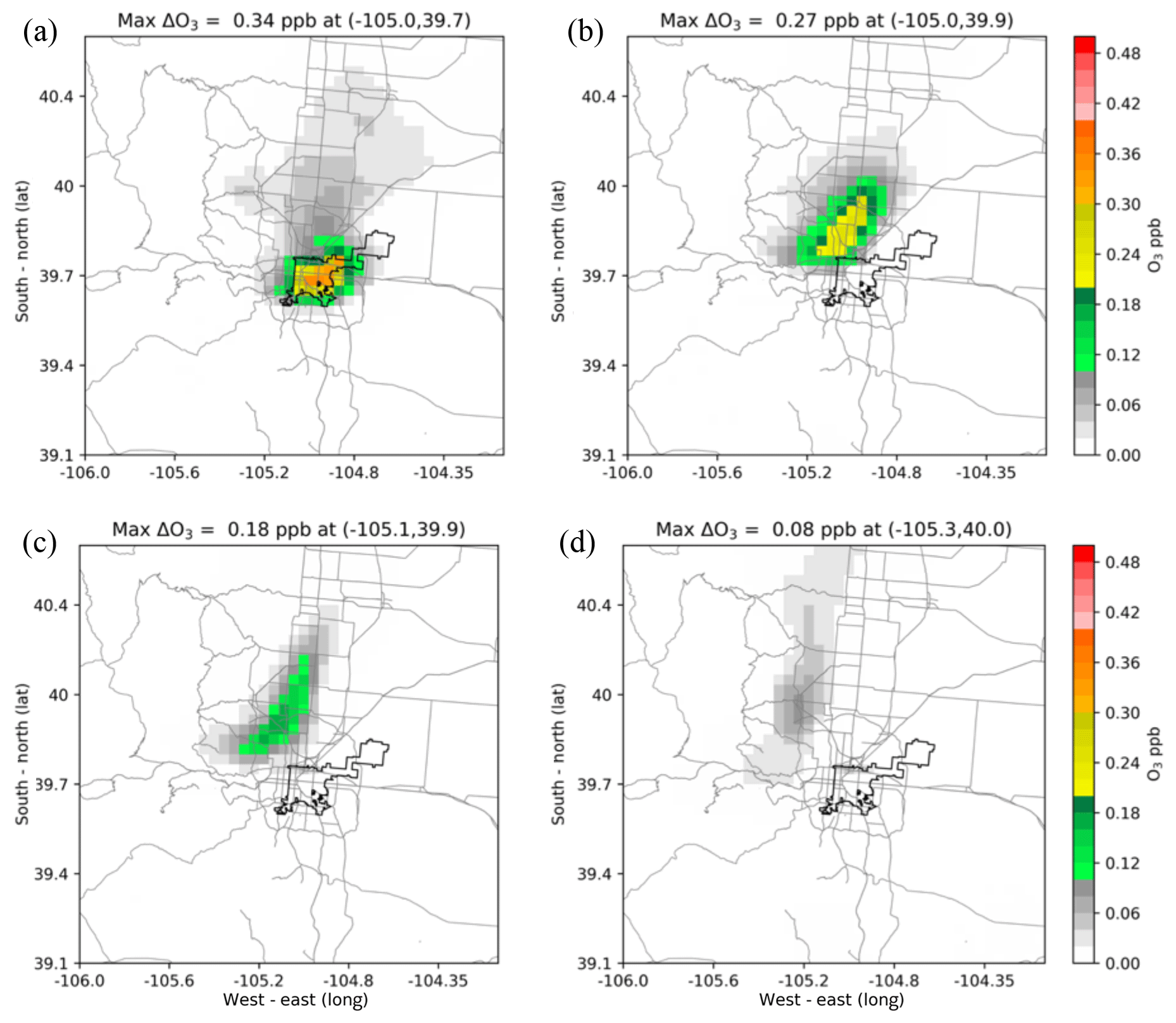
Figure 9For the 3_EC scenario on 18 July 2011 the largest hourly predicted ground-level ozone increases at (a) 09:00 LST, (b) 12:00 LST (i.e., noon), (c) 14:00 LST, and (d) 17:00 LST. The maximum of 0.34 ppb occurred at 09:00 LST.
3.3.1 Ozone impact sensitivity
The maximum modeled daytime hourly ozone increase due to additional CCF emissions occurred on 18 July. Using this day, multiple sensitivity simulations were performed, where CCF emissions from Denver County were incrementally increased up to 3800 t yr−1. Figure 10 shows the increase in terpene emissions from Denver County versus the largest daily increase in hourly ozone concentrations. Figure 10a shows a linear relationship, indicative of a VOC-limited environment, where hourly ozone concentrations are predicted to increase by 1 ppb for every 1000 t yr−1 increase in TERP emissions during the day and 0.85 ppb at night. Also shown is the sensitivity to the MDA8 ozone where there is a 0.30 ppb increase for every 1000 t yr−1 of TERP emissions. According to projected emission inventories provided by the state of Colorado, the ozone non-attainment area was expected to see reductions of 26.4 % of NOx and 24.6 % of VOC emissions by the year 2017 (ENVIRON and Alpine Geophysics, LLC, 2017a). Under these reduced anthropogenic emission scenarios, Fig. 10b shows how ozone would then respond to additional CCF TERP emissions. Figure 10b continues to show a linear relationship, where hourly ozone concentrations are predicted to increase by 1.5 ppb for every 1000 t yr−1 increase in TERP emissions during the day and 1.8 ppb at night. In the future case, the MDA8 ozone increases by 0.38 ppb for every 1000 t yr−1 of TERP emissions. Therefore, Denver will still be VOC-limited and ozone is predicted to be more sensitive to CCF emissions of terpenes.
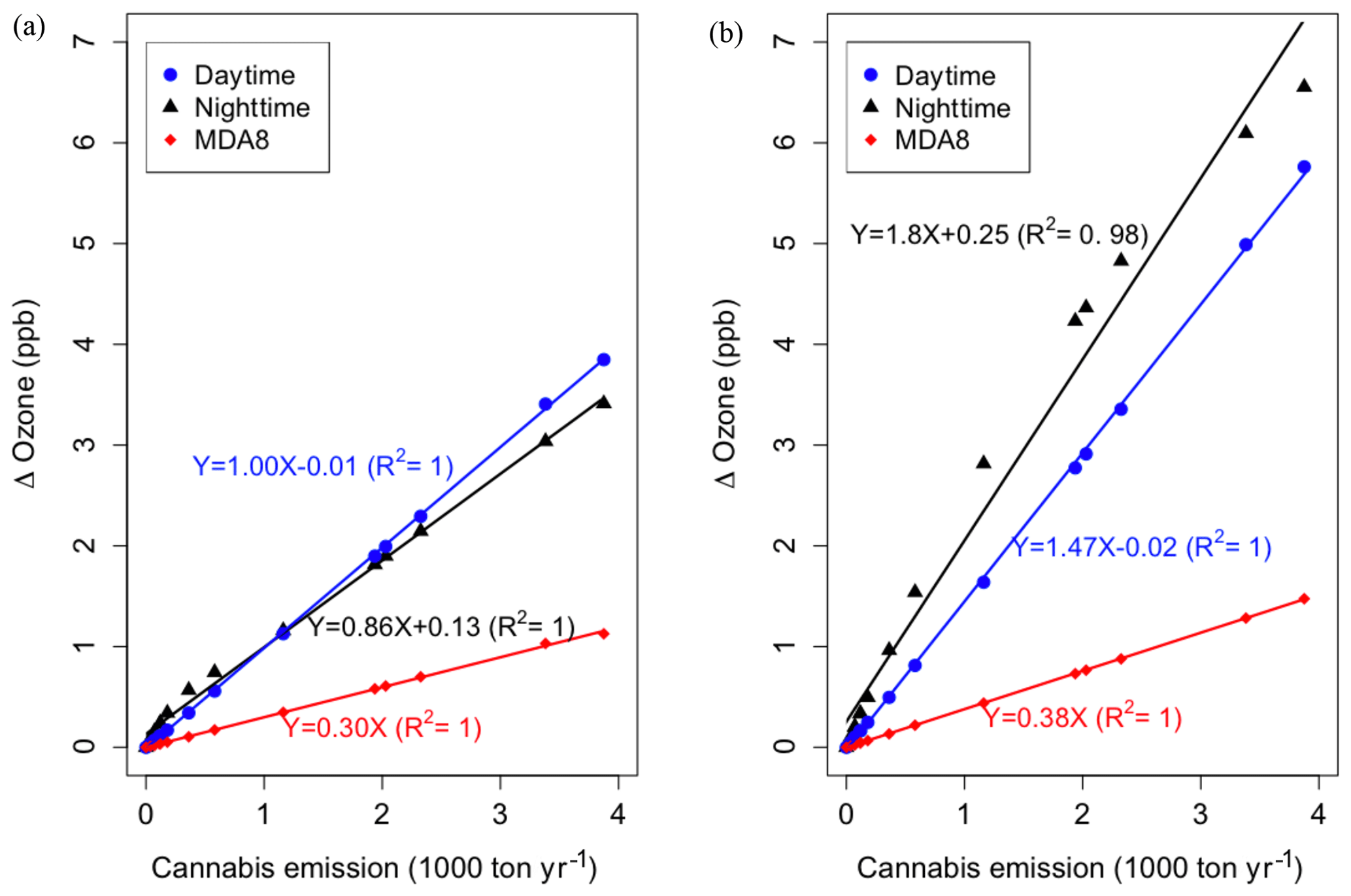
Figure 10For 18 July during (a) 2011 and (b) 2017 the predicted maximum increase in hourly ozone concentrations during daytime hours (06:00–18:00 LST) in blue and nighttime hours (18:00–06:00 LST) in black versus additional terpene emissions in Denver County. Also shown is the response in maximum daily average 8 h ozone concentration (MDA8) in red.
This study provides the first VOC emission inventory to be compiled for the cannabis industry in Colorado, the first time such an analysis has been conducted anywhere in the USA. Given the current state of knowledge of emission rates and growing practices, there are considerable uncertainties in the basic parameters required to build such an inventory. Using realistic bounds on each parameter, we developed seven scenarios, which resulted in estimated emission rates that ranged over an order of magnitude. The highest emissions occur in Denver County, with rates ranging between 36 and 362 t yr−1 for the different scenarios, from a total of 66–652 t yr−1 across Colorado as a whole.
We included these additional terpene emissions in the Comprehensive Air Quality Model with extensions (CAMx), the model used by the state of Colorado for regulatory monitoring and projections. Taking the worst case (3_EC) and median scenario (5_DPW) we consider representative of the current uncertainty upper boundary and future industry expansion, we find that these projected increases in emissions lead to maximum increases in terpene concentrations of up to 5.0 ppb. The largest impacts were seen in locations with the highest terpene emissions coming from CCFs, i.e., in Denver County. We further found that these increases in terpene concentrations affected the local atmospheric chemistry and air quality with ground-level ozone concentrations increasing by as much as 0.34 ppb during the day and 0.67 ppb at night. In general, simulated nighttime increases were higher than those during the daytime, and we take the nighttime of 27–28 July as a case study to further investigate. By applying process analysis (PA), following the evolving plume of VOCs and ozone, we find that the initial reactions of the additional terpenes with OH, NO3, and ozone result in increased formation of peroxyl radicals, which increases the NO-to-NO2 conversion rate and also removes the NOx to generate more NOz product. This effectively reduces the loss of ozone by reaction with NO, increasing the total ozone concentration.
We acknowledge, however, the considerable uncertainties that surround our projections and call for the need for continued efforts to reduce these such that a more accurate assessment of the regional air quality implications of this industry can be made. Future studies that include ambient BVOC measurements are critical for comparisons with model predictions. Additionally, in the model chemical mechanism more accurate and mechanistic representation of terpene species that can reflect the current cannabis emission composition is needed. Currently, the model surrogate TERP, which represents all monoterpene species in the mechanisms, may not represent the precise rate constant for BVOC emissions from cannabis. Further data are needed to reduce uncertainties in emission inventory estimates, specifically those regarding CCF-specific information on plant counts and weight by cultivar and growth stage, coupled with information about the agronomic practices of cannabis cultivation in CCFs. Additional measurements of emission capacities of different cannabis strains at different growth stages are also needed. Further, the emission inventory version is for the year 2011; it may not be suitable to estimate the ozone impacts by the CCF industry.
We chose to focus on ozone since Denver is a moderate non-attainment area with an ozone State Implementation Plan (SIP) (ENVIRON and Alpine Geophysics, LLC, 2017a, b; Colorado, 2018) in accordance with the EPA regulations. But assessments of the impact of these additional terpene emissions on particulate matter (PM2.5) are warranted given the high secondary organic aerosol (SOA) yields of terpenes from 0.3 to 0.8 (Iinuma et al., 2009; Lee et al., 2006; Fry et al., 2014; Slade et al., 2017). It should also be borne in mind that investigations of indoor air quality are needed given the findings of Martyny et al. (2013) and Southwellb et al. (2017) that indoor terpene concentrations reached 50–100 ppb in growth rooms and 30–1600 ppb in flowering rooms, likely initiating intense photochemistry under the powerful growing lamps in use in CCFs.
-
The source code of the CAMx6.10 model can be downloaded on the Environ website: http://www.camx.com (last access: 29 October 2019).
-
The process analysis tools and source codes including PseudoNetCDF, pyPA, and PERMM can be downloaded on GitHub: https://github.com/barronh/pseudonetcdf (Henderson, 2019a), https://github.com/barronh/pypa (Henderson, 2019b), and https://github.com/barronh/permm (Henderson, 2019c).
-
Python 2.7 is used to treat the model output and can be downloaded on the Anaconda Python website: https://www.anaconda.com/distribution/ (last access: 29 October 2019).
-
The air quality model input data and output data (∼2.3 TB) of the WAQS2011b episode for Colorado can be downloaded on the IWDW website: https://views.cira.colostate.edu/iwdw/ (IWDW, 2019).
-
The Colorado highway and Denver County shapefiles can be found on the data.gov website and Denver city website: https://catalog.data.gov/dataset/tiger-line-shapefile-2015-state-colorado-primary-and-secondary-roads-state-based-shapefile (US Census Bureau, 2019) and https://www.denvergov.org/opendata/dataset/city-and-county-of-denver-county-boundary (City and County of Denver, 2019).
The supplement related to this article is available online at: https://doi.org/10.5194/acp-19-13973-2019-supplement.
CTW and WV are lead researchers in this study responsible for research design, experiments, analyzing results, and writing the paper. CW and KA are also co-head researchers and guided the research design, assessed model results, and contributed to writing the paper. JO and PH helped in collecting data and writing the paper. QZR helped to analyze model results and contributed in writing the paper.
The authors declare that they have no conflict of interest.
We want to thank the National Center for Atmospheric Research (NCAR) Advanced Study Program (ASP) and the Atmospheric Chemistry Observations and Modeling (ACOM) Laboratory their support. NCAR is sponsored by the National Science Foundation (NSF). We also thank the Colorado Department of Public Health and Environment (CDPHE) and the Intermountain West Data Warehouse (IWDW) for the model data support. Any opinions, findings, conclusions, or recommendations expressed in this material do not necessarily reflect the views of the National Center for Atmospheric Research (NCAR), the National Science Foundation (NSF), or the Colorado Department of Public Health and Environment (CDPHE). We also thank Kaitlin Urso, Michael Barna, David Hsu, and Grant Josenhans for their invaluable assistance.
This paper was edited by Barbara Ervens and reviewed by two anonymous referees.
Adelman, Z., Shankar, U., Yang, D., and Morris, R.: Western Air Quality Modeling Study Photochemical Grid Model Final Model Performance Evaluation, available at: http://views.cira.colostate.edu/wiki/Attachments/Modeling/WAQS_Base11b_MPE_Final.pdf (last access: 29 October 2019), 2016.
Andreae, M. H., Rhodes, E., Bourgoise, T., Carter, G. M., White, R. S., Indyk, D., Sacks, H., and Rhodes, R.: An Ethical Exploration of Barriers to Research on Controlled Drugs, Am. J. Bioethics, 16, 36–47, https://doi.org/10.1080/15265161.2016.1145282, 2016.
Ashton, C. H.: Pharmacology and effects of cannabis: a brief review, Brit. J. Psychiat., 178, 101–106, https://doi.org/10.1192/bjp.178.2.101, 2001.
Bauer, S., Olson, J., Cockrill, A., van Hattem, M., Miller, L., Tauzer, M., and Leppig, G.: Impacts of Surface Water Diversions for Marijuana Cultivation on Aquatic Habitat in Four Northwestern California Watersheds, Plos One, 10, 25 pp., https://doi.org/10.1371/journal.pone.0120016, 2015.
Borchardt, D.: Forbes-Marijuana Sales Totaled $6.7 Billion In 2016: available at: https://www.forbes.com/sites/debraborchardt/2017/01/03/marijuana-sales-totaled-6-7-billion-in-2016/#2040f22175e3 (last access: 2 May 2019), 2017.
Borgelt, L. M., Franson, K. L., Nussbaum, A. M., and Wang, G. S.: The Pharmacologic and Clinical Effects of Medical Cannabis, Pharmacotherapy, 33, 195–209, https://doi.org/10.1002/phar.1187, 2013.
Butsic, V. and Brenner, J. C.: Cannabis (Cannabis sativa or C. indica) agriculture and the environment: a systematic, spatially-explicit survey and potential impacts, Environ. Res. Lett., 11, 10 pp., https://doi.org/10.1088/1748-9326/11/4/044023, 2016.
Carah, J. K., Howard, J. K., Thompson, S. E., Gianotti, A. G. S., Bauer, S. D., Carlson, S. M., Dralle, D. N., Gabriel, M. W., Hulette, L. L., Johnson, B. J., Knight, C. A., Kupferberg, S. J., Martin, S. L., Naylor, R. L., and Power, M. E.: High Time for Conservation: Adding the Environment to the Debate on Marijuana Liberalization, Bioscience, 65, 822–829, https://doi.org/10.1093/biosci/biv083, 2015.
Carter, W. P. L.: Development of the SAPRC-07 chemical mechanism and updated ozone reactivity scales, available at: https://www.engr.ucr.edu/~carter/SAPRC/saprc07 (last access: 29 October 2019), 2010.
CDOR: Licensees – Marijuana Enforcement Division, available at: https://www.colorado.gov/pacific/enforcement/med-licensed-facilities (last access: 2 May 2019), 2018a.
CDOR: Marijuana Sales Reports, available at: https://www.colorado.gov/pacific/revenue/colorado-marijuana-sales-reports (last access: 2 May 2019), 2018b.
CDOR: MED Resources and Statistics, available at: https://www.colorado.gov/pacific/enforcement/med-resources-and-statistics, last access: 2 May 2019.
CDPHE: Denver Metro Area & North Front Range 8-Hour Ozone State Implementation Plan (SIP), available at: http://www.colorado.gov/airquality/documents/deno308/, last access: 2 May 2009.
City and County of Denver: Open Data Catalog, available at: https://www.denvergov.org/opendata/dataset/city-and-county-of-denver-county-boundary, last access: 29 October 2019.
Colorado RAQC: The Colorado State Implementation Plan Planning Process: An Overview of Clean Air Act Requirements for SIP Development and Approval, Reginal Air Quality Council, available at: https://raqc.egnyte.com/dl/SMXBbYwYdO/StateImplementationPlanSummaries2018.pdf_ (last access: 29 October 2019), 2018.
Crick, E., Haase, H. J., and Bewley-Taylor, D.: Legally regulated cannabis markets in the US: Implications and possibilities, Global Drug Policy Observatory, available at: https://www.swansea.ac.uk/media/Leg%20Reg%20Cannabis%20digital%20new-1.pdf (last access: 29 October 2019), 2013.
Eisenstein, M.: Medical marijuana: Showdown at the cannabis corral, Nature, 525, S15–S17; https://doi.org/10.1038/525S15a, 2015.
ENVIRON: CAMx User's Guide Version 6.10, available at: http://www.camx.com/files/camxusersguide_v6-10.pdf (last access: 2 May 2019), 2013.
ENVIRON and Alpine Geophysics, LLC: Denver Metro/North Front Range 2017 8-Hour Ozone State Implementation Plan: 2017 Attainment Demonstration Modeling Final Report, Regional Air Quality Council, available at: http://views.cira.colostate.edu/wiki/Attachments/Source%20Apportionment/Denver/Denver_2017SIP_2017AttainDemo_Finalv1.pdf (last access: 29 October 2019), 2017a.
ENVIRON and Alpine Geophysics, LLC: Attainment Demonstration Modeling for the Denver Metro/North Front Range 2017 8-Hour Ozone State Implementation Plan, Western Air Quality Study – Intermountain West Data Warehouse, available at: https://raqc.egnyte.com/dl/gFls58KHSM/Model_Protocol_Denver_RAQC_2017SIPv4.pdf_8.pdf_ (last access: 29 October 2019), 2017b.
Esri, HERE, TomTom, Intermap, increment P Corp., GEBCO, USGS, FAO, NPS, NRCAN, GeoBase, IGN, Kadaster NL, Ordnance Survey, Esri Japan, METI, Esri China (Hong Kong), swisstopo, MapmyIndia, and the GIS User Community: World Topographic Map, available at: https://services.arcgisonline.com/ArcGIS/rest/services/World_Topo_Map/MapServer, (last access: 29 October 2019), 2013.
Fischedick, J. T., Hazekamp, A., Erkelens, T., Choi, Y. H., and Verpoorte, R.: Metabolic fingerprinting of Cannabis sativa L, cannabinoids and terpenoids for chemotaxonomic and drug standardization purposes, Phytochemistry, 71, 2058–2073, https://doi.org/10.1016/j.phytochem.2010.10.001, 2010.
Fry, J. L., Draper, D. C., Barsanti, K. C., Smith, J. N., Ortega, J., Winkler, P. M., Lawler, M. J., Brown, S. S., Edwards, P. M., Cohen, R. C., and Lee, L.: Secondary organic aerosol formation and organic nitrate yield from NO3 oxidation of biogenic hydrocarbons, Environ. Sci. Technol., 48, 11944–11953, https://doi.org/10.1021/es502204x, 2014.
Fuentes, J. D., Lerdau, M., Atkinson, R., Baldocchi, D., Bottenheim, J. W., Ciccioli, P., Lamb, B., Geron, C., Gu, L., Guenther, A., Sharkey, T. D., and Stockwell, W.: Biogenic hydrocarbons in the atmospheric boundary layer: A review, B. Am. Meteorol. Soc., 81, 1537–1575, https://doi.org/10.1175/1520-0477(2000)081<1537:bhitab>2.3.co;2, 2000.
Guenther, A. B., Jiang, X., Heald, C. L., Sakulyanontvittaya, T., Duhl, T., Emmons, L. K., and Wang, X.: The Model of Emissions of Gases and Aerosols from Nature version 2.1 (MEGAN2.1): an extended and updated framework for modeling biogenic emissions, Geosci. Model Dev., 5, 1471–1492, https://doi.org/10.5194/gmd-5-1471-2012, 2012.
Hartman, M., Humphreys, H., Burack, J., Lambert, K., and Martin, P.: MED 2017 Annual Update, Colorado Department of Revenue, available at: https://www.colorado.gov/pacific/sites/default/files/MED2017AnnualUpdate.pdf (last access: 29 October 2019), 2018a.
Hartman, M., Humphreys, H., Burack, J., Lambert, K., and Martin, P.: MED 2018 Mid-Year Update, Colorado Department of Revenue, available at: https://www.colorado.gov/pacific/sites/default/files/2018%20Mid%20Year%20Update.pdf (last access: 29 October 2019), 2018b.
Henderson, B. H.: PseudoNetCDF like Netcdf except for many scientific format backends, available at: https://github.com/barronh/pseudonetcdf, last access: 29 October 2019a.
Henderson, B. H.: pyPA, available at: https://github.com/barronh/pypa, last access: 29 October 2019b.
Henderson, B. H.: Python-based Environment for Reaction Mechanisms/Mathematics, available at: https://github.com/barronh/permm, last access: 29 October 2019c.
Henderson, B. H., Jeffries, H. E., Kim, B. U., and Vizuete, W.: The Influence of Model Resolution on Ozone in Industrial Volatile Organic Compound Plumes, Japca J. Air Waste Ma., 60, 1105–1117, https://doi.org/10.3155/1047-3289.60.9.1105, 2010.
Henderson, B. H., Kimura, Y., McDonald-Buller, E., Allen, D. T., and Vizuete, W.: Comparison of Lagrangian Process Analysis tools for Eulerian air quality models, Atmos. Environ., 45, 5200–5211, https://doi.org/10.1016/j.atmosenv.2011.06.005, 2011.
Hillig, K. W.: A chemotaxonomic analysis of terpenoid variation in Cannabis, Biochem. Syst. Ecol., 32, 875–891, https://doi.org/10.1016/j.bse.2004.04.004, 2004.
Hites, R. A. and Turner, A. M.: Rate Constants for the Gas-Phase beta-Myrcene plus OH and Isoprene plus OH Reactions as a Function of Temperature, Int. J. Chem. Kinet., 41, 407–413, https://doi.org/10.1002/kin.20413, 2009.
Hood, L. V. S., Dames, M. E., and Barry, G. T.: Headspace Volatiles of Marijuana, Nature, 242, 402–403, 1973.
IDCP: The Social Impact Of Drug Abuse,, United Nations International Drug Control Programme, available at: https://www.unodc.org/pdf/technical_series_1995-03-01_1.pdf (last access: 29 October 2019), 1995.
Iinuma, Y., Boge, O., Keywood, M., Gnauk, T., and Herrmann, H.: Diaterebic Acid Acetate and Diaterpenylic Acid Acetate: Atmospheric Tracers for Secondary Organic Aerosol Formation from 1,8-Cineole Oxidation, Environ. Sci. Technol., 43, 280–285, https://doi.org/10.1021/es802141v, 2009.
IWDW: Modeling platforms, available at: https://views.cira.colostate.edu/iwdw/, last access: 29 October 2019.
Laothawornkitkul, J., Taylor, J. E., Paul, N. D., and Hewitt, C. N.: Biogenic volatile organic compounds in the Earth system, New Phytol., 183, 27–51, https://doi.org/10.1111/j.1469-8137.2009.02859.x, 2009.
LCB: Washington State Liquor and Cannabis Board, available at: https://lcb.wa.gov (last access: 2 May 2019), 2017.
Lee, A., Goldstein, A. H., Keywood, M. D., Gao, S., Varutbangkul, V., Bahreini, R., Ng, N. L., Flagan, R. C., and Seinfeld, J. H.: Gas-phase products and secondary aerosol yields from the ozonolysis of ten different terpenes, J. Geophys. Res.-Atmos., 111, 18, https://doi.org/10.1029/2005jd006437, 2006.
Marchini, M., Charvoz, C., Dujourdy, L., Baldovini, N., and Filippi, J. J.: Multidimensional analysis of cannabis volatile constituents: Identification of 5,5-dimethyl-1-vinylbicyclo 2.1.1 hexane as a volatile marker of hashish, the resin of Cannabis sativa L, J. Chromatogr. A, 1370, 200–215, https://doi.org/10.1016/j.chroma.2014.10.045, 2014.
Martyny, J. W., Serrano, K. A., Schaeffer, J. W., and Van Dyke, M. V.: Potential Exposures Associated with Indoor Marijuana Growing Operations, J. Occup. Environ. Hyg., 10, 622–639, https://doi.org/10.1080/15459624.2013.831986, 2013.
METRC: Marijuana Enforcement Tracking Reporting Compliance: available at: https://www.metrc.com (last access: 2 May 2019), 2018.
Mills, E.: The carbon footprint of indoor Cannabis production, Energ. Policy, 46, 58–67, https://doi.org/10.1016/j.enpol.2012.03.023, 2012.
Ortega, J., Turnipseed, A., Guenther, A. B., Karl, T. G., Day, D. A., Gochis, D., Huffman, J. A., Prenni, A. J., Levin, E. J. T., Kreidenweis, S. M., DeMott, P. J., Tobo, Y., Patton, E. G., Hodzic, A., Cui, Y. Y., Harley, P. C., Hornbrook, R. S., Apel, E. C., Monson, R. K., Eller, A. S. D., Greenberg, J. P., Barth, M. C., Campuzano-Jost, P., Palm, B. B., Jimenez, J. L., Aiken, A. C., Dubey, M. K., Geron, C., Offenberg, J., Ryan, M. G., Fornwalt, P. J., Pryor, S. C., Keutsch, F. N., DiGangi, J. P., Chan, A. W. H., Goldstein, A. H., Wolfe, G. M., Kim, S., Kaser, L., Schnitzhofer, R., Hansel, A., Cantrell, C. A., Mauldin, R. L., and Smith, J. N.: Overview of the Manitou Experimental Forest Observatory: site description and selected science results from 2008 to 2013, Atmos. Chem. Phys., 14, 6345–6367, https://doi.org/10.5194/acp-14-6345-2014, 2014.
Pfister, G. G., Reddy, P. J., Barth, M. C., Flocke, F. F., Fried, A., Herndon, S. C., Sive, B. C., Sullivan, J. T., Thompson, A. M., Yacovitch, T. I., Weinheimer, A. J., and Wisthaler, A.: Using Observations and Source-Specific Model Tracers to Characterize Pollutant Transport During FRAPPE and DISCOVER-AQ, J. Geophys. Res.-Atmos., 122, 10474–10502, https://doi.org/10.1002/2017jd027257, 2017.
Rice, S. and Koziel, J. A.: Characterizing the Smell of Marijuana by Odor Impact of Volatile Compounds: An Application of Simultaneous Chemical and Sensory Analysis, Plos One, 10, 11, https://doi.org/10.1371/journal.pone.0144160, 2015a.
Rice, S. and Koziel, J. A.: The relationship between chemical concentration and odor activity value explains the inconsistency in making a comprehensive surrogate scent training tool representative of illicit drugs, Forensic Sci. Int., 257, 257–270, https://doi.org/10.1016/j.forsciint.2015.08.027, 2015b.
Ruiz, L. H. and Yarwood, G.: Interactions between organic aerosol and NOy: Influence on oxidant production, the University of Texas at Austin, and ENVIRON International Corporation, Novato, CA, available at: http://aqrp.ceer.utexas.edu/projectinfoFY12_13/12-012/12-012%20Final%20Report.pdf (last access: 29 October 2019), 2013.
Seinfeld, J. H. and Pandis, S. N.: Atmospheric Chemistry and Physics: From Air Pollution to Climate Change, 262, table 6.5, 2006.
Slade, J. H., de Perre, C., Lee, L., and Shepson, P. B.: Nitrate radical oxidation of γ-terpinene: hydroxy nitrate, total organic nitrate, and secondary organic aerosol yields, Atmos. Chem. Phys., 17, 8635–8650, https://doi.org/10.5194/acp-17-8635-2017, 2017.
Southwellb, J., Wena, M., and Jobsona, B., Thomas Spokane Regional Clean Air Agent (SRCAA) Marijuana Air Emissions Sampling & Testing Project, Inland Northwest Chapter AWMA, Washington State, October 2017.
Stith, S. S. and Vigil, J. M.: Federal barriers to Cannabis research, Science, 352, 1182–1182, https://doi.org/10.1126/science.aaf7450, 2016.
Sznitman, S. R. and Zolotov, Y.: Cannabis for Therapeutic Purposes and public health and safety: A systematic and critical review, Int. J. Drug Policy, 26, 20–29, https://doi.org/10.1016/j.drugpo.2014.09.005, 2015.
Topshelfdata: Topshelfdata, available at: https://www.topshelfdata.com/listing/any_license/state/wa (last access: 2 May 2019), 2017.
Turner, C. E., Elsohly, M. A., and Boeren, E. G.: Constituents of Sannabis-Sativa L.17. A review of the natural constituents, J. Nat. Prod., 43, 169–234, https://doi.org/10.1021/np50008a001, 1980.
UNC-IE and ENVIRON: Three-State Air Quality Modeling Study (3SAQS) Final Modeling Protocol 2008 Emission & Air Quality Modeling Platform, available at: http://views.cira.colostate.edu/wiki/Attachments/Modeling/3SAQS_2008_Modeling_Protocol_Final.pdf (last access: 29 October 2019), 2013.
UNC-IE and ENVIRON: Three-State Air Quality Modeling Study CAMx Photochemical Grid Model Final Model Performance Evalution, Western Air Quality Study – Intermountain West Data Warehouse, available at: http://views.cira.colostate.edu/wiki/Attachments/Modeling/3SAQS_Base08b_MPE_Final_30Sep2014.pdf (last access: 29 October 2019), 2014.
US Census Bureau: TIGER/LINE Shapefile, 2015, state, Colorado, Primary and Secondary Roads State-based Shapefile, available at: https://catalog.data.gov/dataset/tiger-line-shapefile-2015-state-colorado-primary-and-secondary-roads-state-based-shapefile, last access: 29 October 2019.
USEPA: Criteria Air Pollutants, available at: https://www.epa.gov/criteria-air-pollutants (last access: 2 May 2019), 2016.
USEPA: 8-Hour Ozone (2008) Nonattainment Areas by State/County/Area, available at: https://www3.epa.gov/airquality/greenbook/hncty.html (last access: 2 May 2019), 2017.
Wang, C.-T., Wiedinmyer, C., Ashworth, K., Harley, P. C., Ortega, J., and Vizuete, W.: Leaf enclosure measurements for determining volatile organic compound emission capacity from Cannabis spp., Atmos. Environ., 199, 80–87, https://doi.org/10.1016/j.atmosenv.2018.10.049, 2019.
WAQS: IWDW-WAQS Wiki, available at: http://views.cira.colostate.edu/wiki/#WAQS (last access: 2 May 2019), 2017.
Wen, M., Southwell, J., and Jobson, B. T.: Identification of Compounds Responsible for Marijuana Growing Operation Odor Complaints in the Spokane Area, Pacific Northwest International Section 57th annual conference, Boise, Idaho, 2017.
WHO: The health and social effects of nonmedical cannabis use, World Health Organisation, ISBN 978 92 4 151024 0, available at: http://www.who.int/substance_abuse/publications/msbcannabis.pdf (last access: 29 October 2019), 2016.