the Creative Commons Attribution 4.0 License.
the Creative Commons Attribution 4.0 License.
 | 05 Nov 2019
Investigating the assimilation of CALIPSO global aerosol vertical observations using a four-dimensional ensemble Kalman filter
Yueming Cheng
Daisuke Goto
Nick A. J. Schutgens
Guangyu Shi
Teruyuki Nakajima
Aerosol vertical information is critical to quantify the influences of aerosol on the climate and environment; however, large uncertainties still persist in model simulations. In this study, the vertical aerosol extinction coefficients from the Cloud-Aerosol Lidar with Orthogonal Polarization (CALIOP) onboard the Cloud–Aerosol Lidar and Infrared Pathfinder Satellite Observation (CALIPSO) are assimilated to optimize the hourly aerosol fields of the Non-hydrostatic ICosahedral Atmospheric Model (NICAM) online coupled with the Spectral Radiation Transport Model for Aerosol Species (SPRINTARS) using a four-dimensional local ensemble transform Kalman filter (4-D LETKF). A parallel assimilation experiment using bias-corrected aerosol optical thicknesses (AOTs) from the Moderate Resolution Imaging Spectroradiometer (MODIS) is conducted to investigate the effects of assimilating the observations (and whether to include vertical information) on the model performances. Additionally, an experiment simultaneously assimilating both CALIOP and MODIS observations is conducted. The assimilation experiments are successfully performed for 1 month, making it possible to evaluate the results in a statistical sense. The hourly analyses are validated via both the CALIOP-observed aerosol vertical extinction coefficients and the AOT observations from MODIS and the AErosol RObotic NETwork (AERONET). Our results reveal that both the CALIOP and MODIS assimilations can improve the model simulations. The CALIOP assimilation is superior to the MODIS assimilation in modifying the incorrect aerosol vertical distributions and reproducing the real magnitudes and variations, and the joint CALIOP and MODIS assimilation can further improve the simulated aerosol vertical distribution. However, the MODIS assimilation can better reproduce the AOT distributions than the CALIOP assimilation, and the inclusion of the CALIOP observations has an insignificant impact on the AOT analysis. This is probably due to the nadir-viewing CALIOP having much sparser coverage than MODIS. The assimilation efficiencies of CALIOP decrease with increasing distances of the overpass time, indicating that more aerosol vertical observation platforms are required to fill the sensor-specific observation gaps and hence improve the aerosol vertical data assimilation.
- Article
(22375 KB) - Full-text XML
-
Supplement
(39599 KB) - BibTeX
- EndNote


Aerosols have significant impacts on air quality, climate change, radiation balance, and the hydrological cycle (Charlson et al., 1992; Huang et al., 2014; Liu et al., 2011, 2014; Nakajima et al., 2001; Ramanathan et al., 2001). Aerosols may also contribute to regional differences in historical warming rates (Huang et al., 2017). Due to the large uncertainties in the parameterizations of various aerosol processes such as emission, transport, and deposition, it is still a challenge for models to accurately quantify the effects of aerosols on the Earth system (Huneeus et al., 2011; Liu et al., 2015; Jia et al., 2015; Myhre et al., 2013; Sato et al., 2018; Sato and Suzuki, 2019; Textor et al., 2006). Aerosol data assimilation, which makes optimal use of both observations and numerical simulations to obtain the best possible estimates of aerosol behaviors, is an emerging way to obtain accurate predictions and characterizations of atmospheric aerosol and its influence.
Recently, aerosol assimilation studies have been conducted to improve model simulation performances, generally using optimal interpolation, variational, or ensemble-based methods. The assimilated aerosol observations commonly include spaceborne or ground-based aerosol optical thicknesses (AOTs) from the POLarization and Directionality of the Earth's Reflectances (POLDER) (Generoso et al., 2007), Moderate Resolution Imaging Spectroradiometer (MODIS) (Dai et al., 2014a; Di Tomaso et al., 2017; Hyer et al., 2011; Liu et al., 2011; Yin et al., 2016a, b; Yumimoto et al., 2011, 2017; Zhang and Reid, 2006), Himawari-8 (Dai et al., 2019; Yumimoto et al., 2018), AERONET (Schutgens et al., 2010a, b), and multi-sensors (Rubin et al., 2017; Zhang et al., 2014). Although assimilating AOTs can strongly constrain the horizontal distributions of aerosol burdens, it is limited in terms of improving vertical information on aerosols. The vertical distribution of aerosols is a combined characteristic of atmospheric transport patterns, residence times in the atmosphere, and the efficiency of the vertical energy exchange (Koffi et al., 2012; Yu et al., 2010), which shows large diversities of up to an order of magnitude among models (Textor et al., 2006). Reductions of the large uncertainties in aerosol vertical distributions are of crucial importance for the accurate evaluation of the aerosol impacts on the Earth system, such as the aerosol direct effect (Oikawa et al., 2013, 2018) and the aerosol indirect effect (Liu et al., 2019a, b).
Apart from AOTs, aerosol vertical information such as the aerosol extinction coefficient is another variable for aerosol assimilation. Uno et al. (2008) and Yumimoto et al. (2008) developed a four-dimensional variational (4D-Var) assimilation system with a regional dust model to assimilate the retrieved extinction coefficient from the ground-based National Institute for Environment Studies (NIES) lidar network for investigating Asian dust. Due to the limited spatiotemporal frequencies of the aerosol vertical observations and the noise signal from the lidar observations, aerosol vertical assimilation is still at an initial stage. The Cloud–Aerosol Lidar and Infrared Pathfinder Satellite Observation (CALIPSO), which carried the Cloud-Aerosol Lidar with Orthogonal Polarization (CALIOP) instrument with high horizontal and vertical resolutions, exhibits great potential for reducing the uncertainties in the global spatiotemporal distributions of aerosols, especially the vertical profiles. The CALIPSO satellite provides an outstanding opportunity to study aerosol vertical information, especially over high elevations and harsh climate regions (Huang et al., 2007). Based on the CALIOP observations, a new technique was developed to distinguish anthropogenic dust from natural dust to explore the effects of anthropogenic emissions on radiative forcing, climate change, and air quality (Huang et al., 2015). A coupled 2D–3D-Var system, which assimilated CALIOP-retrieved aerosol extinction profiles for 2 weeks was developed by Zhang et al. (2011). Zhang et al. (2014) also conducted multi-sensor experiments and found that the inclusion of CALIOP data can improve the aerosol vertical distribution and hence forecasted advection. Variational data assimilation systems use the precalculated static model error covariance matrix, whereas an ensemble-based Kalman filter (EnKF) can generate a flow-dependent model error covariance matrix to better represent the background error (Evensen, 1994). Flow-dependent model errors are calculated by ensemble simulations. Sekiyama et al. (2010) initially applied a four-dimensional local ensemble transform Kalman filter (4-D LETKF) to assimilate CALIOP-attenuated backscattering coefficients with an analysis at the center of the 48 h assimilation window. However, hourly aerosol analyses using the 4-D LETKF approach can provide more accurate aerosol features to investigate the environmental and climate effects of aerosols (Dai et al., 2019).
Therefore, in the present study, we apply 4-D LETKF and an aerosol model called the Spectral Radiation Transport Model for Aerosol Species (SPRINTARS) online coupled with a new dynamical atmospheric model called the Non-hydrostatic ICosahedral Atmosphere Model (NICAM) to generate hourly aerosol horizontal and vertical analyses for 1 month using the CALIOP aerosol extinctions. The results are validated using both the CALIOP extinctions and the MODIS and AERONET AOT observations. To the best of our knowledge, this is the first study to conduct hourly aerosol vertical extinction assimilation using the four-dimensional ensemble Kalman method for 1 month.
The observation data used in this study are described in Sect. 2. The forward model and the data assimilation methodology are described in Sect. 3. Section 4 presents the assimilation results and their validation. The discussion and main conclusions achieved in this study are shown in Sects. 5 and 6, respectively.
2.1 CALIOP
CALIOP, a spaceborne two-wavelength polarization lidar that is the prime payload instrument carried by the CALIPSO satellite, has probed the high-resolution vertical structures and properties of clouds and aerosols since 2006 (Winker et al., 2007). CALIPSO flies as one of five satellites in the so-called “A-train” constellation of satellites, and all the satellites are in a 705 km sun-synchronous polar orbit with a 16 d repeat cycle. During both day and night, CALIOP continuously provides vertical profiles of the aerosol extinction coefficient at 532 and 1064 nm, with a uniform spatial resolution of 60 m vertically and 5 km horizontally over an altitude range of −0.5 to 30 km. In this study, we only use the aerosol extinction coefficients at 532 nm in the CALIPSO lidar level 2 (L2) version 4.10 aerosol profile products over the altitude range below 10 km for assimilation (http://www-calipso.larc.nasa.gov/, last access: 15 September 2019). The CALIPSO lidar level 2 version 4.10 Vertical Feature Mask (VFM) products, which consist of information on the feature type and subtype, are used for aerosol discrimination. AOTs from the CALIPSO level 3 version 3 aerosol profile monthly products at 2∘ × 5∘ resolution for cloud-free conditions in November from 2006 to 2016 are also used.
2.2 MODIS
MODIS aboard NASA's Terra and Aqua satellites is making near-global daily observations of the Earth in a wide spectral range (0.41–15 µm) (Remer et al., 2005). In this study, the United States Naval Research Laboratory (NRL) quality-assured and controlled MODIS level 3 AOT products are also used for data assimilation. The NRL MODIS AOTs are based on the MODIS level 2 aerosol products and aggregated to a 1∘ × 1∘ grid with reduced biases and error variances for use in near-real-time data assimilation processes (Zhang and Reid, 2006). The datasets consist of 6-hourly gridded AOTs and error estimates four times per day (00:00, 06:00, 12:00, and 18:00 UTC). Since the representation of the observations is considered during the development of the NRL MODIS datasets and the NRL MODIS AOTs have been subjected to extensive quality assurance and quality check procedures for aerosol assimilation (Zhang and Reid, 2006; Zhang et al., 2008), we directly use the NRL MODIS AOTs and the corresponding AOT uncertainties every 6 h at 1∘ without further operation. The MODIS Aqua Collection 6.1 level 2 Dark Target (DT) and Deep Blue (DB) merged AOT observations at 550 nm are used to validate the model simulations. The DT and DB merged AOT provides a more gap-filled dataset than the observation, which is only retrieved from the individual algorithms (https://modis.gsfc.nasa.gov, last access: 15 September 2019) (Levy et al., 2013; Sayer et al., 2014). The Community Intercomparison Suite (CIS) tool (Watson-Parris et al., 2016), which was developed to allow for the straightforward comparison of remote sensing, in situ, and model data, is used to aggregate the level 2 MODIS AOTs at 10 km and 5 min resolution to produce the hourly MODIS AOTs at 2∘ × 2∘ for comparison. The AOTs from the MODIS Aqua Collection 6.1 (C6.1) level 3 monthly aerosol products with 1∘ × 1∘ resolution in November from 2006 to 2016 are also used.
2.3 AERONET
The AErosol RObotic NETwork (AERONET; http://aeronet.gsfc.nasa.gov/, last access: 15 September 2019) version 3 (V3) data provide globally distributed near-real-time observations of aerosol spectral optical thickness at nominal standard aerosol wavelengths of 340, 380, 440, 500, 675, 870, 1020, and 1640 nm (Holben et al., 1998; Giles et al., 2019). Due to the both availability of the AOTs at 440 nm in most AERONET sites and the model calculations, we directly use the level 2 cloud-screened AERONET AOTs at 440 nm for the validation. The AERONET-retrieved instantaneous AOTs within the preceding 1 h are averaged to calculate the hourly mean AOTs for comparison.
3.1 Model
A global three-dimensional aerosol transport model, SPRINTARS (Takemura, 2003; Takemura et al., 2000, 2009), online coupled with NICAM (Satoh et al., 2005, 2008, 2014; Tomita and Satoh, 2004) is used as the forward model to predict the aerosol spatial and temporal evolutions. The major tropospheric aerosols including dust, sea salt, sulfate, and carbonaceous aerosols are simulated in NICAM–SPRINTARS considering the main aerosol processes including emissions, advection, and dry and wet deposition. A three-dimensional icosahedral grid advection scheme preserving monotonicity and consistency with continuity for aerosol transport is adopted in NICAM (Niwa et al., 2011). The dust and sea salt aerosols, spanning wide size ranges, are divided into 10 and 4 bins for transport, respectively, whereas the sulfate and carbonaceous aerosols are predicted using the bulk modal method (Takemura et al., 2000). Aerosol–cloud–radiation interactions are included in the aerosol-coupled version of NICAM (Sato et al., 2018). In this study, NICAM–SPRINTARS is set up with a homogeneous horizontal resolution of about 223 km and a vertical resolution of 40 layers from the surface to approximately 40 km of altitude. The vertical grid spacing is approximately 160 m near the surface, and the spaces exponentially increase to approximately 1320 m around 16 km. NICAM is successfully applied to produce a high-resolution global simulation with a horizontal resolution of about 0.87 km (Miyamoto et al., 2013), indicating the potential application of a sub-kilometer global aerosol simulation and data assimilation when the computer resources are available. With the stretched-grid system, NICAM can also be used to run partially high-resolution simulations in the object regions (Goto et al., 2015). Therefore, there is future potential to extend the present assimilation method to fine-scale regional analyses using the stretched-grid system implemented in NICAM (Uchida et al., 2016, 2017). The biomass burning and anthropogenic emission inventories for BC, OC, and SO2 used in this study are from the Global Fire Emissions Database (GFEDv3.1; van der Werf et al., 2010) and the Hemispheric Transport of Air Pollution (HTAP; Janssens-Maenhout et al., 2015) as in Dai et al. (2019). The dust and sea salt emission fluxes are both mainly dependent on the near-surface wind speeds (Dai et al., 2018; Takemura et al., 2009). The meteorological fields in NICAM are nudged by the reanalysis data every 6 h from the NCEP Final (FNL) analysis (https://rda.ucar.edu/datasets/ds083.2/, last access: 15 September 2019) to reduce the influences of uncertainties in the meteorological conditions on the aerosol simulations.
3.2 Data assimilation methodology
The 4-D LETKF (Dai et al., 2019; Hunt et al., 2007) assimilation system of NICAM–SRPINTARS is used to assimilate CALIOP vertical extinctions and NRL MODIS AOT observations, which is an extension of the LETKF to assimilate asynchronous observations. In this section, we briefly describe the basic scheme of LETKF; more details on the LETKF algorithm and its implementation can be found in Hunt et al. (2007). The LETKF determines the analysis ensemble mean locally in the space spanned by the ensemble with the following formula:
where and Xb represent the background (forecast) ensemble mean and background ensemble perturbations, respectively. The weight vector is obtained as
where the matrix R is the observation error covariance matrix; yo and represent the assimilated observations and the ensemble mean background observations; the ensemble background observations are calculated by applying the observation operator H to the ensemble member state vector xb(i) as yb(i)=H(xb(i)); and the matrix Yb represents ensemble background observation perturbations, whose ith column is , with k ensemble members. The analysis error covariance in ensemble space is calculated as
where I is the identity matrix, and the analysis ensemble perturbations Xa are obtained as
whose ith column is . The analysis ensemble by adding to each of the columns of Xa forms the optimal initial conditions for the ensemble forecast to produce the background for the next analysis.
To generate the hourly aerosol analysis, LETKF requires hourly switching between the model ensemble forward simulations and the assimilation of synchronous observations. However, as shown in Fig. 1, 4-D LETKF considers approximate model trajectories by linear combinations of the background ensemble trajectories and compares these approximate trajectories with the observations taken over the assimilation time window (Hunt et al., 2007), which can assimilate asynchronous observations and avoid frequent switching between assimilations and model ensemble forecasts. With respect to the assimilation window time of 24 h, the system performs the ensemble forecast for 24 h and outputs at every hour time slot within the time window. Based on the innovations throughout the assimilation window, the ensemble mean background observations and the background ensemble perturbation matrix are formed at the various time slots when the observations are available and then vertically concatenated to form a combined background observation mean and perturbation matrix Yb. Following the LETKF formulas, all the innovations and Yb throughout the day are used for the calculation of the weight matrix and Wa. The weights determined at the end of a short assimilation window (e.g., 24 h) should be valid throughout the window (Dai et al., 2019; Hunt et al., 2007; Kalnay and Yang, 2010). To perform a linear combination of ensemble trajectories, the same is then applied to the state vector at every hour time slot throughout the assimilation window to obtain the hourly analysis ensemble mean (Di Tomaso et al., 2017; Dai et al., 2019). The analyzed aerosol fields at the last slot can then directly serve as the initial conditions for the next 24 h of forward simulation; therefore, our implementation of 4-D LETKF can also avoid the multiple use of one observation without overlapping the ensemble forecasts between adjacent assimilation cycles. One advantage of 4-D LETKF is the localization technique, which allows the local analyses to choose different linear combinations of the ensemble members in local regions using a prescribed localization scale to explore a much higher-dimensional space than the ensemble space and reduce spurious correlations with distance (Hunt et al., 2007). Furthermore, localization enables parallel computation to reduce computational cost (Yumimoto et al., 2018). The horizontal and vertical localizations are both performed in the observational error covariance matrix by the physical distance to avoid discontinuity in the analysis (Miyoshi et al., 2007). The observational error covariance matrix is calculated as the observation uncertainties multiplied by the inverse of the horizontal and vertical localization factors so that the effect of observations on the analysis decreases with increasing distance. The horizontal and vertical localization factors are both defined following Gaussian shapes as , where σ represents the localization length and the r is the distance of observations from the local patch center. Although the Gaussian function has infinitely long tails, we truncate the tails to simulate the 5th-order piecewise rational function by Gaspari and Cohn (1999), which is a widely used localization weighting function in EnKF studies (Miyoshi et al., 2007). The 5th-order rational function drops to zero at and we do not assimilation observations beyond this distance. We do not apply temporal localization in this study since our results indicate that temporally remote asynchronous observations within 24 h have limited influence on the analysis. To better reduce the computational resources and limit the model information to a few modes only, the subspecies of the SPRINTARS-predicted aerosols are summarized into a fine (carbonaceous and sulfate aerosol) and a coarse (sea salt and dust aerosol) mode for assimilation as in Schutgens et al. (2010a). The modeled aerosol fine and coarse mass mixing ratios are hourly optimized using the hourly aggregated observations during the assimilation window, and the mass mixing ratios after data assimilation for each subspecies are determined from their relative fractions before assimilation (Dai et al., 2019). The observation operators we used to map the model state vector into the aerosol extinction coefficient σ and the AOT observation space at wavelength λ are calculated as and , where Mj represents the simulated aerosol dry mass concentration in each model level j, and β represents the prescribed aerosol mass extinction coefficient (Dai et al., 2014b).
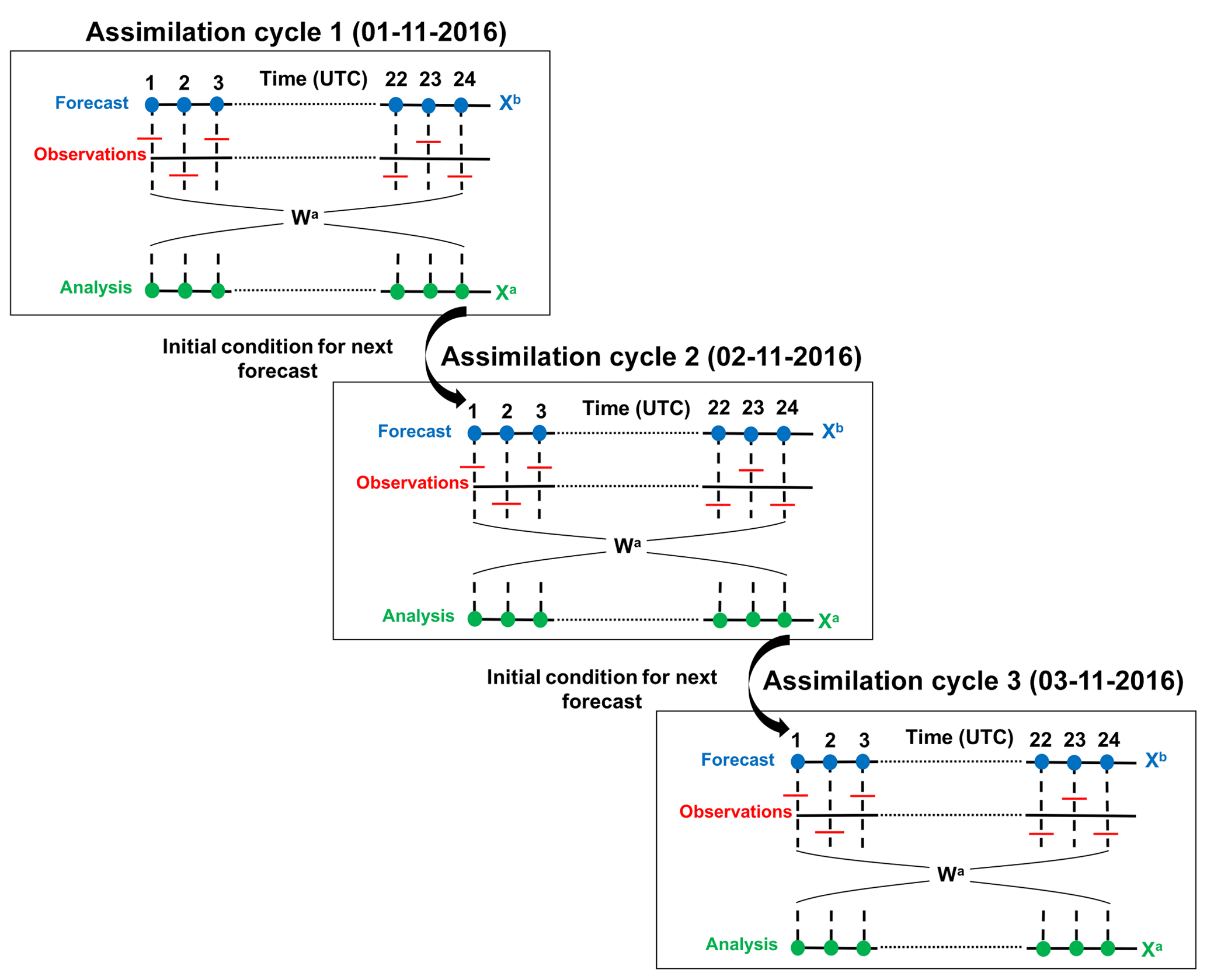
Figure 1Schematic illustrating the three assimilation cycles of 4-D LETKF. Hourly observations are shown as red line segments for the each 24 h assimilation cycle. The blue dots represent the 24 h forecast that are hourly output. The green dots represent the hourly analysis within the 24 h assimilation window.
A total of 668 CALIPSO orbit paths in November 2016 are obtained and used for the aerosol data assimilation. To identify the aerosol signals and screen out the cloud signals, we applied several quality-control procedures to remove noisy or highly uncertain observations before aggregating the profile data. The quality controls include the following: (1) the vertical feature mask must be determined as aerosols; (2) the cloud–aerosol discrimination (CAD) score must be lower than −80, indicating high confidence in discriminating aerosols; (3) the extinction quality control (QC) flag must be equal to 0 or 1 (Young and Vaughan, 2009); (4) the extinction coefficient must be greater than 0 and less than 100 km−1; and (5) the uncertainty of the extinction coefficient must be lower than 10 km−1, indicating a stable iteration.
After the quality control of the data, we aggregate the original CALIOP extinction coefficients to the model grid boxes. Firstly, we perform an hourly horizontal aggregation to the model horizontal resolution of about 2∘ × 2∘ at the CALIOP observation level (i.e., every 0.06 km) using the mean value of all the reasonable sub-grid observations within ±30 min. The CALIOP extinction observations within the range of μ±σ are used for the average, where μ and σ represent the mean and the standard deviation of the sub-grid observations in the aggregation cell, respectively. To avoid assimilation of sub-grid features likely to create anomalies in the horizontal 2∘ grid cell (Schutgens et al., 2017), the number of retrievals used within the 2∘ grid cell must also be greater than 20, and the coefficient of extinction variations within the grid cell (i.e., the standard deviation and mean) must be less than 0.5, similar to Zhang and Reid (2006). Then, the horizontally regridded observations within each model layer are averaged to serve as the assimilated observations. The observation uncertainties are assumed to be 20 % of the mean aerosol extinctions in reference to Winker et al. (2007) and Sekiyama et al. (2010).
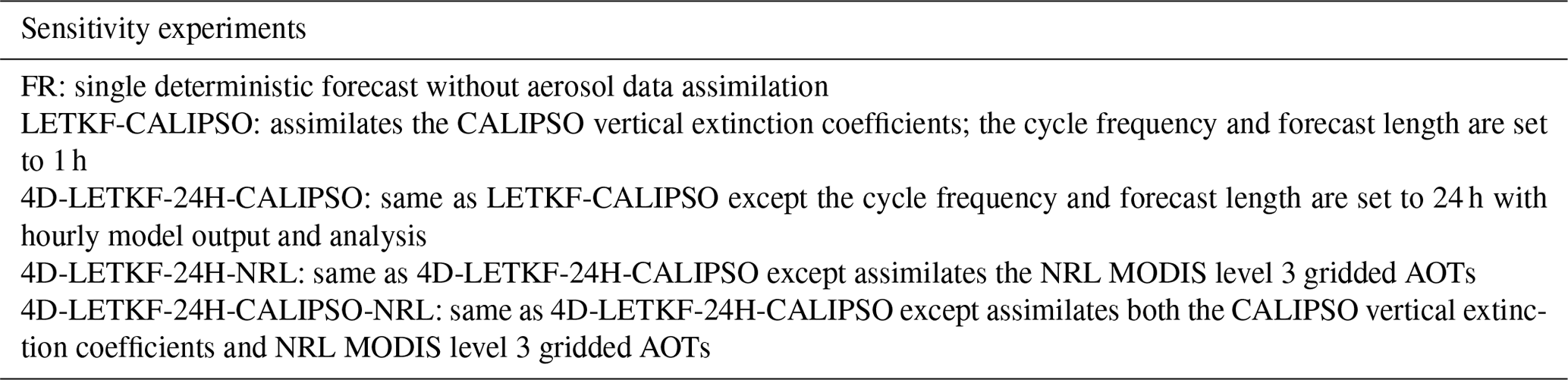
As summarized in Table 1, a total of five numerical experiments are conducted for this study. Data assimilation is initiated at 00:00 UTC on 1 November 2016 and terminated at 00:00 UTC on 1 December 2016. The initial condition at 00:00 UTC on 1 November is prepared by a 1-month simulation executed by NICAM–SPRINTARS without any aerosol data assimilation as a spin-up. A single deterministic simulation with the default model configuration is performed as a reference in November 2016 (a free-running experiment, referred to as an FR experiment hereafter). Two experiments assimilating the CALIOP vertical extinction coefficients with time windows of 1 and 24 h (hereafter called LETKF-CALIPSO and 4D-LETKF-24H-CALIPSO, respectively) are performed to investigate the influences of the assimilation time window on the hourly aerosol analysis. Combined with the 4D-LETKF-24H-CALIPSO experiment, two more assimilation experiments are designed to investigate the impacts of assimilating the observations (and whether to include vertical information) and the impacts of multi-sensor data assimilation on the model simulations. The first one assimilates the NRL MODIS AOTs including no vertical aerosol information (4D-LETKF-24H-NRL experiment hereafter). In the second one, the CALIOP vertical extinction coefficients and NRL MODIS AOTs are assimilated simultaneously. The assimilation system parameters are based on several tuning experiments as discussed in Sect. 5. A total of 20 members with spatiotemporally perturbed aerosol emissions are used to generate the model ensemble simulations. The perturbation factors follow the same lognormal distributions as those used in Dai et al. (2019), except the uncertainty of sea salt is assumed as 500 % following Yumimoto and Takemura (2011). This is due to the emission fluxes of sea salt are still not well known, which can span a factor about 20 for the different source functions even excluding outliers (Grythe et al., 2014). The horizontal and vertical localization lengths are set as 200 km and one model layer (increasing by altitude), respectively. To prevent filter divergence, multiplicative inflation with a fixed factor of 1.1 is performed on the background ensemble following Sekiyama et al. (2010).
Table 1Experimental design for the sensitivity tests in this study.
The results in the FR, LETKF-CALIPSO, 4D-LETKF-24H-CALIPSO, and 4D-LETKF-24H-NRL experiments are firstly compared with the assimilated CALIOP vertical extinctions and the NRL MODIS AOTs as self-verification. In order to investigate the similarities and the differences among the four assimilation experiments, we use three independent observations (i.e., AERONET AOTs, independent MODIS Aqua AOTs, and independent daytime CALIOP aerosol extinctions) to validate the simulated AOTs and aerosol extinctions, respectively. To quantify the model performances, statistical criteria (Boylan and Russell, 2006; Willmott et al., 2012; Yumimoto et al., 2017), including the mean fractional bias (MFB), the mean fractional error (MFE), the root mean square error (RMSE), the correlation coefficient (CORR), and the index of agreement (IOA), are calculated between the simulated results and observations. Because of the small differences between the AOTs at 532 and 550 nm, i.e., between 2 % and 4 % for typical Ångström exponents of 0.5 to 1 (Kittaka et al., 2011), we directly use the modeled aerosol extinction coefficients at 550 nm to compare with the observations at 532 nm.
4.1 Internal check of the analysis
4.1.1 Internal check of the analysis with the assimilated CALIOP aerosol extinctions
In this section, we only analyze the performance of the experiments assimilating CALIOP extinctions using the assimilated CALIOP extinction coefficients at 532 nm as a sanity or internal check (Benedetti et al., 2009). Figure 2a–j show the scatter plots of the assimilated CALIOP extinction coefficients versus the simulated ones over the global land and ocean, and Fig. 2k–l further show the probability distribution functions (PDFs) of collocated forecast-minus-observation deviations in the FR experiment and analysis-minus-observation deviations in the assimilation experiments. Based on the model performance evaluation statistical metrics (i.e., MFB, MFE, RMSE, CORR, and IOA), the two CALIOP assimilation experiments are evidently better than the FR experiment, especially over the ocean regions. The CORR values are 0.317 and 0.365 over the global land and ocean for the FR experiment, whereas the LETKF-CALIPSO and 4D-LETKF-24H-CALIPSO experiments significantly improve the CORRs over global land (ocean) to 0.600 (0.792) and 0.668 (0.782), respectively. The distributions of the extinction coefficient deviations in the FR experiment show systematically negative biases, indicating the model tends to underestimate the extinction coefficients in most of the world. Obviously, the PDFs over both the land and ocean in the two CALIOP assimilation experiments are symmetrical to the value of 0 and more squeezed with higher peaking. Merely 13.56 % (27.49 %) and 15.73 % (32.03 %) of the extinction coefficient deviations over the land and ocean are within ±0.01(±0.02) in the FR experiment, while 37.89 % (56.30 %) and 51.15 % (73.91 %) of the deviations are achieved within ±0.01(±0.02) in the LETKF-CALIPSO experiment. The performances of the 4D-LETKF-24H-CALIPSO experiment are generally comparable to those of the LETKF-CALIPSO experiment. This indicates that the weights determined at the end of the 24 h assimilation window are valid to optimize the ensemble trajectories and the temporally remote asynchronous observations within 24 h have limited influence on the analysis. The elimination of the strong underestimations over both the global land and ocean in the two CALIOP assimilation experiments provides a positive sanity check of the assimilation system.
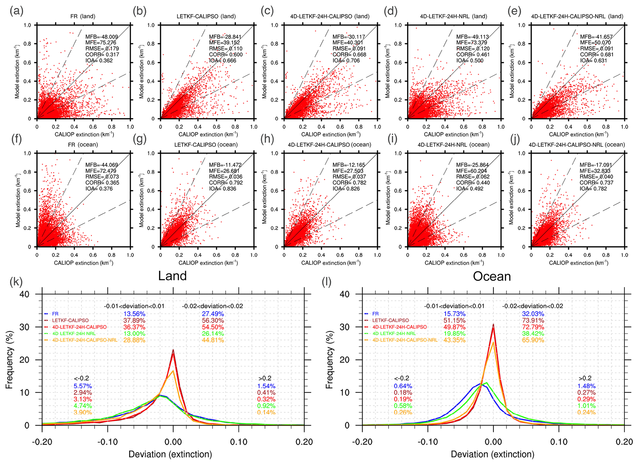
Figure 2Scatter plots of the CALIOP (Cloud-Aerosol Lidar with Orthogonal Polarization) hourly aerosol extinction coefficients at 532 nm (km−1) versus the simulated ones at 550 nm over the global land (a, b, c, d, e) and ocean (f, g, h, i, j) during November 2016 for the FR, LETKF-CALIPSO, 4D-LETKF-24H-CALIPSO, 4D-LETKF-24H-NRL, and 4D-LETKF-24H-CALIPSO-NRL experiments. The solid black line is the 1:1 line and the dashed black lines correspond to the 1:2 and 2:1 lines. MFB, MFE, RMSE, CORR, and IOA represent the mean fractional bias, the mean fractional error, the root mean square error, the correlation coefficient, and the index of agreement, respectively. Frequency distributions of deviations (modeled extinction coefficients minus the CALIOP-observed ones) over the global land (k) and ocean (l). The percentages of deviations between ±0.01, ±0.02, , and >0.2 are also shown.
To further assess the effects of assimilating CALIOP aerosol extinctions on the aerosol column simulations over different aerosol regimes, we choose 13 regions and classify them into four groups according to their surface aerosol emission regimes (Huang et al., 2013). The column-integrated aerosol extinctions from 0 to 10 km of altitude is used for comparison. The four groups are dominated by biomass burning smoke, dust, industrial pollution, and marine aerosols (Fig. 3a). As shown in Fig. 3b–f, the modeled column-integrated extinctions are compared with the CALIOP ones over the 13 selected regions. All five statistical metrics of the LETKF-CALIPSO and 4D-LETKF-24H-CALIPSO experiments are superior to those of the FR experiment, indicating that the spatiotemporal distributions of the column-integrated aerosol characteristics are closer to those of the CALIOP observations after the CALIOP assimilation. The modeled column-integrated extinctions in the FR experiment show negative biases compared to CALIOP for 11 out of the 13 regions, reaching up to 42 % and 66 % for the SEA and SAM regions in the biomass burning regime, respectively. With the CALIOP assimilation, the modeled column-integrated extinctions are generally increased over all the underestimated regions. The RMSE value decreases from 0.028 to 0.020 (0.022) and the CORR value increases from 0.871 in the FR experiment to 0.955 (0.963) in the LETKF-CALIPSO (4D-LETKF-24H-CALIPSO) experiment. In addition to the evaluation of the modeled mean column-integrated extinctions in Fig. 3b–f, we further employ the Taylor graph (Taylor, 2001) to quantitatively assess the pattern correspondence between the simulated and observed fields on the regional level (Fig. 3g). The correlation coefficient, the centered pattern root mean square (RMS) difference, and the ratios of the modeled and observed standard deviation are all indicated by a single point on a two-dimensional plot. The ratios of the modeled and observed standard deviation in the FR experiment range from 0.30 over the SAM region to 2.05 over the ECN region, while the upper bounds are significantly down to 1.59 and 1.19 in the LETKF-CALIPSO and 4D-LETKF-24H-CALIPSO experiments. The regions with obviously underestimated dispersion are less improved by the aerosol data assimilation, as shown by the relatively small variations of the lower bounds. This is due to the aerosol extinctions generally being more strongly underestimated over the regions with underestimated dispersion, making it difficult to generate enough model errors by perturbing aerosol emissions. Thus, the observational errors are too large relative to the model errors, which translates to a reduced impact of the observation on the model state.
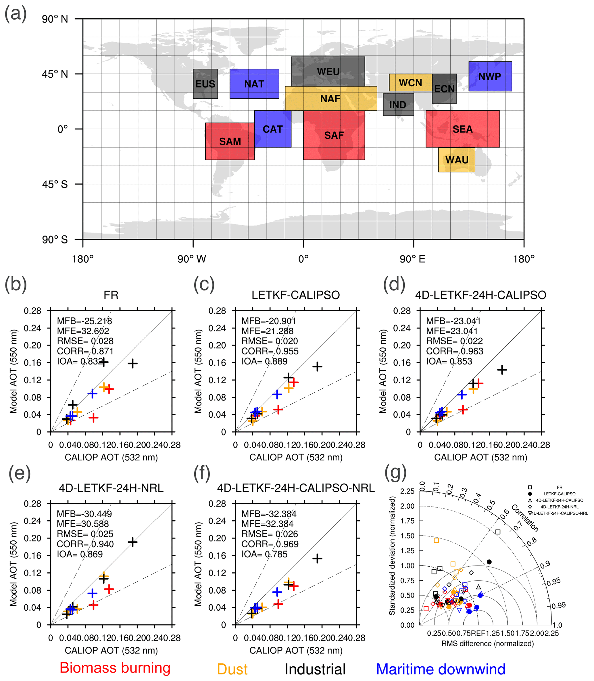
Figure 3(a) The 13 domains selected for regional analysis in this study. The red, orange, black, and blue boxes indicate source regions of biomass burning smoke (SAM, SAF, and SEA), dust (NAF, WCN, and WAU), industrial pollution (IND, ECN, WEU, and EUS), and the outflow maritime regions downwind of major dust and industrial pollution sources (NWP, NAT, and CAT), respectively. Scatter plots of the simulated regionally averaged monthly mean column-integrated aerosol extinctions at 550 nm versus the collocated CALIOP ones at 532 nm over the 13 selected regions during November 2016 for the FR (b), LETKF-CALIPSO (c), 4D-LETKF-24H-CALIPSO (d), 4D-LETKF-24H-NRL (e), and 4D-LETKF-24H-CALIPSO-NRL (f) experiments. (g) A Taylor graph describing the column-integrated aerosol extinctions in the five experiments compared with the observed ones.
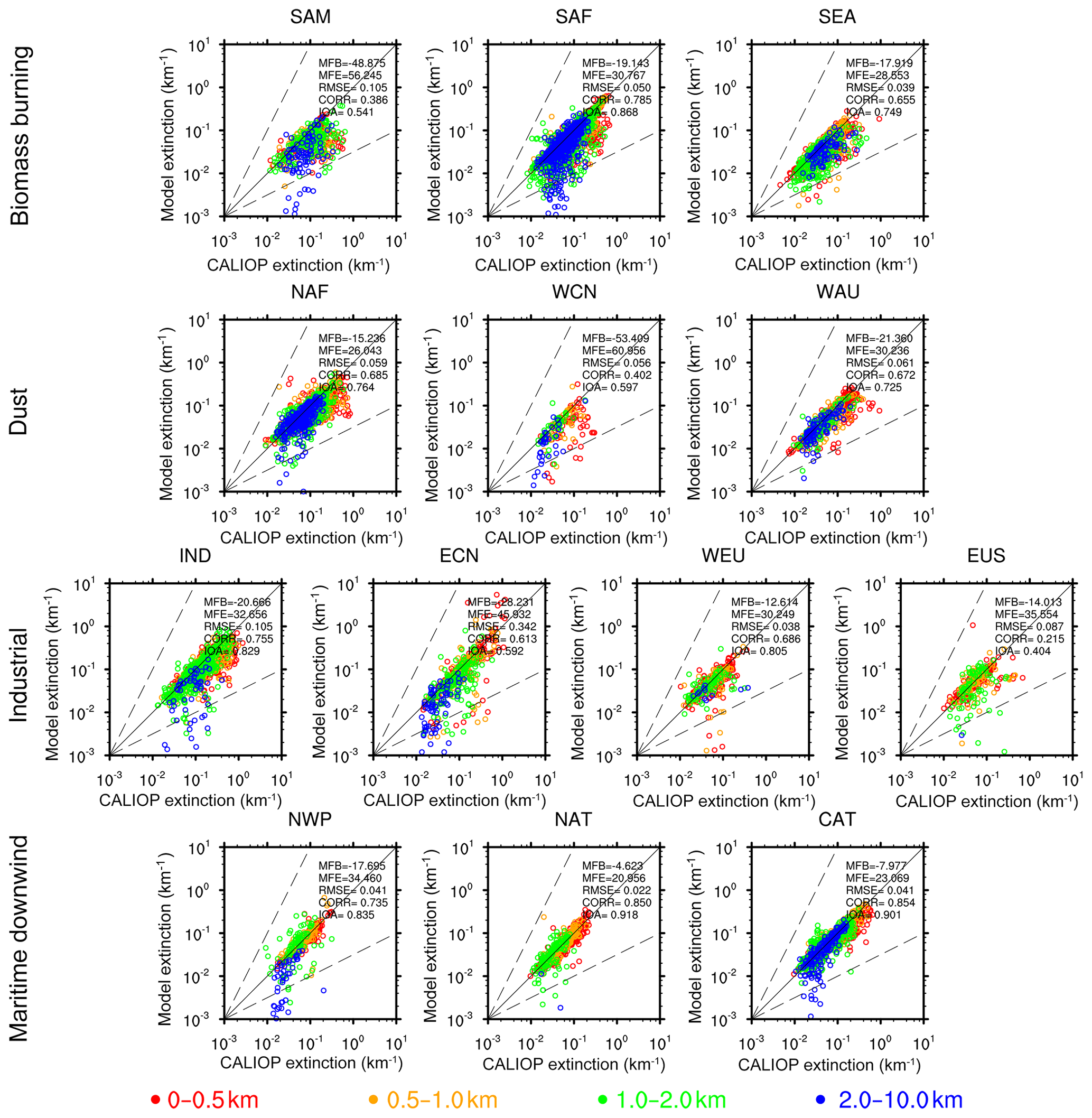
Figures 4–6 show scatter plots of the modeled and CALIOP-observed hourly extinction coefficients within 0–10 km over the 13 regions for the FR, LETKF-CALIPSO, and 4D-LETKF-24H-CALIPSO experiments, respectively. The aerosol extinctions are classified into four altitude ranges (0–0.5 km, 0.5–1.0 km, 1.0–2.0 km, and 2.0–10.0 km) to further investigate the effects of the CALIOP assimilation on the simulations of aerosol vertical characteristics. The statistical metrics of the LETKF-CALIPSO and 4D-LETKF-24H-CALIPSO experiments are clearly superior to those of the FR experiment over all 13 regions, and those of the 4D-LETKF-24H-CALIPSO experiment are generally comparable to those of the LETKF-CALIPSO experiment. The slight differences between the two CALIOP assimilation experiments are induced by the effects of asynchronous observations on the hourly analysis. The large negative MFB values reveal that the FR experiment tends to underestimate the aerosol extinction coefficients over all three biomass burning regions, especially over the SAM region. The improvements of the CALIOP assimilation on the simulated extinction coefficients over the SAM region are not so obvious compared to the other two regions. This is probably due to the emission fluxes of biomass burning aerosols over the SAM region being clearly underestimated, leading to an underestimation of the model uncertainty, and hence the analysis underweights the observations. The extinction coefficients in the free atmosphere (2–10 km) of the LETKF-CALIPSO and 4D-LETKF-24H-CALIPSO experiments are more narrowly distributed along the 1:1 line than those in the boundary layer (0–2 km) for the SAF and SEA regions. The lower observed extinction coefficients associated with the lower observation errors at higher altitude and the high injections of fire products induce model uncertainties that are relatively larger than the observation ones; hence, the analysis underweights the model. Dust is a predominant component of aerosol in the NAF, WCN, and WAU regions, where the main deserts in the world are located. The improvements of the simulated extinction coefficients by the CALIOP assimilation in the NAF and WAU regions are more obvious than those in the WCN region. The proportions of observations within 1–2 km (2–10 km) for the NAF, WCN, and WAU regions are 37 % (11 %), 22 % (22 %), and 24 % (14 %), respectively. This indicates that the dust aerosols emitted from the desert in western China have higher possibilities of being transported at a relatively high altitude than those emitted from the desert in North Africa (Ginoux et al., 2001; Huang et al., 2009). Therefore, dust emissions from western China will have wider impacts on downwind areas than those of NAF, leading to a smaller model spread over the dust source regions of WCN; hence, the analysis underweights the observations. In the WAU region, the significant overestimations of the extinction coefficients over 1 km in the FR experiment are probably caused by a simulated dust storm (Dai et al., 2019), and the CALIOP assimilation corrects this overestimation. In the IND, ECN, WEU, and EUS regions, urban and industrial aerosols are the major part of the aerosol loadings (Penning de Vries et al., 2015). The aerosols in this regime, especially over ECN, mainly exist below 2 km as indicated by the relatively large extinction coefficients. It is apparent that the CALIOP assimilation can significantly improve the model performances of simulated extinction coefficients over all four anthropogenic aerosol regions. The NWP, NAT, and CAT regions are oceanic regions located downwind of the major dust and industrial pollution sources. Thus, these oceanic regions are substantially influenced by the mixture of ocean emissions, ship exhaust, and transported continental emissions (Sorooshian and Duong, 2010). It is apparent the CALIOP assimilation over the maritime downwind regime has the highest assimilation efficiencies among the four regimes. A common problem that the analyses generally fail to correct is the significantly underestimated extinction coefficients found over all four aerosol regimes. This is probably due to insufficient emissions leading to underestimated extinctions and model errors, and thus the analysis underweights the observation.

Figure 4Scatter plots of the hourly modeled aerosol extinction coefficients at 550 nm (km−1) versus the CALIOP-observed ones at 532 nm over the 13 selected regions during November 2016 for the FR experiment.

The vertical profiles of the monthly and regional averaged aerosol extinctions and the ratios between the modeled and observed standard deviations of the aerosol extinctions and the collocated CALIOP retrievals over the 13 regions are shown in Fig. 7. We ignore the levels at which the number of available CALIPSO observations is less than 10. With respect to the biomass burning regime, the FR experiment underestimates the aerosol extinction profiles over all the available levels of all three biomass burning regions. This indicates that the biomass burning emissions in November 2016 are probably stronger than those used in this study. The shape of the simulated extinction profile over the SEA region in the FR experiment is generally consistent with the CALIOP observations, whereas the FR experiment fails to simulate the descending trend of the extinction coefficients over the SAF region. The CALIOP assimilation experiments decrease the negative biases over all three biomass burning regions and achieve the descending trend of the extinction coefficients over the SAF region. Moreover, the ratios of the simulated and observed standard deviation over the SAF region with the CALIOP assimilation are closer to 1 than those in the FR experiment. With respect to the dust regime, it is found that the CALIOP assimilation has marginal impacts on the vertical profiles except over the WAU region. The simulated profile of extinction coefficients over WAU is apparently more comparable to the CALIOP-observed one than that in the FR experiment, and the significantly descending trend in the CALIOP observations below 1 km is successfully reproduced in the experiments with CALIOP assimilation. The simulated ascending trend of the aerosol extinctions above 2.5 km over the WAU in the FR experiment is corrected by the CALIOP assimilation, which is probably due to the elimination of the simulated dust event. There are limited improvements with data assimilation over the WCN region due to the limited observations to be assimilated. For the NAF region, the CALIOP assimilation induces a slightly larger negative bias of the vertical profile than that of the FR experiment. This is due to the fact that the assimilation is more efficient at reducing positive biases than negative ones. This situation is also found in the IND region. Over the ECN region, it is obvious that the FR experiment significantly overestimates the extinction coefficients below 1 km. This is due to the fact that the anthropogenic emission inventories used in this study are based on the year 2010, whereas the anthropogenic emissions over ECN have been significantly reduced due to national regulations on anthropogenic emissions. The CALIOP assimilation successfully eliminates the significant overestimations below 1 km. Over the WEU region, the CALIOP assimilation experiments reproduce the vertical profile of the aerosol extinctions much better than those in the FR experiment. Over the EUS region, the overestimations of the extinction coefficients over 1 km (mainly contributed by sulfate aerosols) are correctly amended by the data assimilation. Over the NWP and NAT regions, although the FR experiment simulates totally opposite vertical distributions of extinction coefficients to those of the CALIOP observations, the CALIOP assimilation experiments reproduce the profile of the CALIOP observations successfully. The significant discrepancies of the aerosol profiles over the maritime downwind regions between the FR and the CALIOP assimilation experiments are due to the relatively sufficient spread of sea salt emissions below 2 km (figure not shown for brevity).
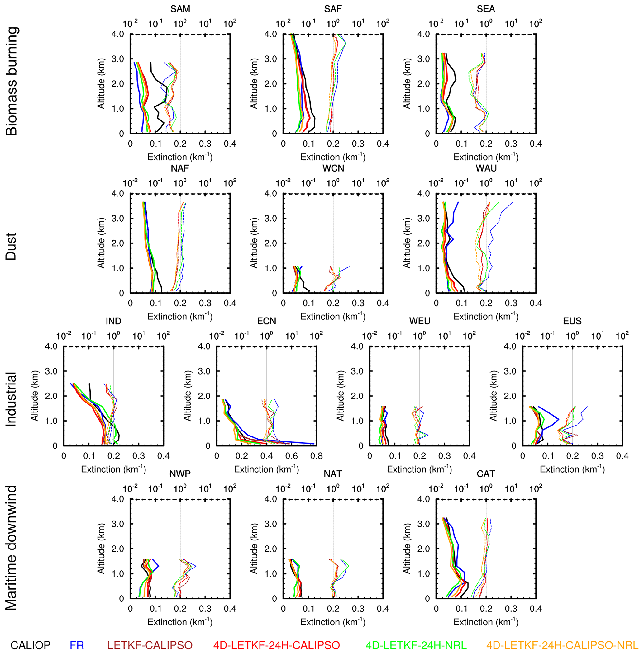
Figure 7Regionally averaged monthly mean vertical profiles of the simulated aerosol extinction coefficients for the five experiments at 550 nm (km−1) and the CALIOP-observed ones at 532 nm (solid lines), with the ratios between the simulated and observed standard deviations (dashed line) over the 13 selected regions during November 2016.
4.1.2 Internal check of the analysis with the assimilated NRL MODIS AOTs
In this section, we perform a self-verification of the simulated hourly AOTs in the 4D-LETKF-24H-NRL experiment over the whole month through a comparison with the assimilated NRL MODIS AOTs.
Figure 8a–j show the spatial distributions of the biases and RMSEs between the simulated and NRL MODIS AOTs at 550 nm. In Fig. 8k, we also present PDF plots of the AOT deviations between the simulated hourly AOTs and the NRL MODIS-observed ones over the whole month. The 4D-LETKF-24H-NRL experiment significantly reduces the positive biases and the associated high RMSEs over southeast China and Australia. As shown in Fig. S1 in the Supplement, the improvements over southeast China mostly benefit from reductions of sulfate, as well as OC and BC aerosols, and the improvements over Australia mostly benefit from reductions of natural dust aerosols. The significant underestimation of simulated AOTs in the FR experiment over northern India is corrected by the increments of anthropogenic aerosols after the MODIS assimilation. The distribution of the AOT deviations relative to the NRL MODIS observations for the FR experiment is negatively biased, and the 4D-LETKF-24H-NRL experiment is superior to the FR experiment as indicated by the reduced biases and the peaks in 0. The frequencies of AOT deviation within ±0.05 (±0.10) in the 4D-LETKF-24H-NRL experiment are 71.83 % (90.32 %), whereas those in the FR experiment are 64.73 % (83.29 %) .
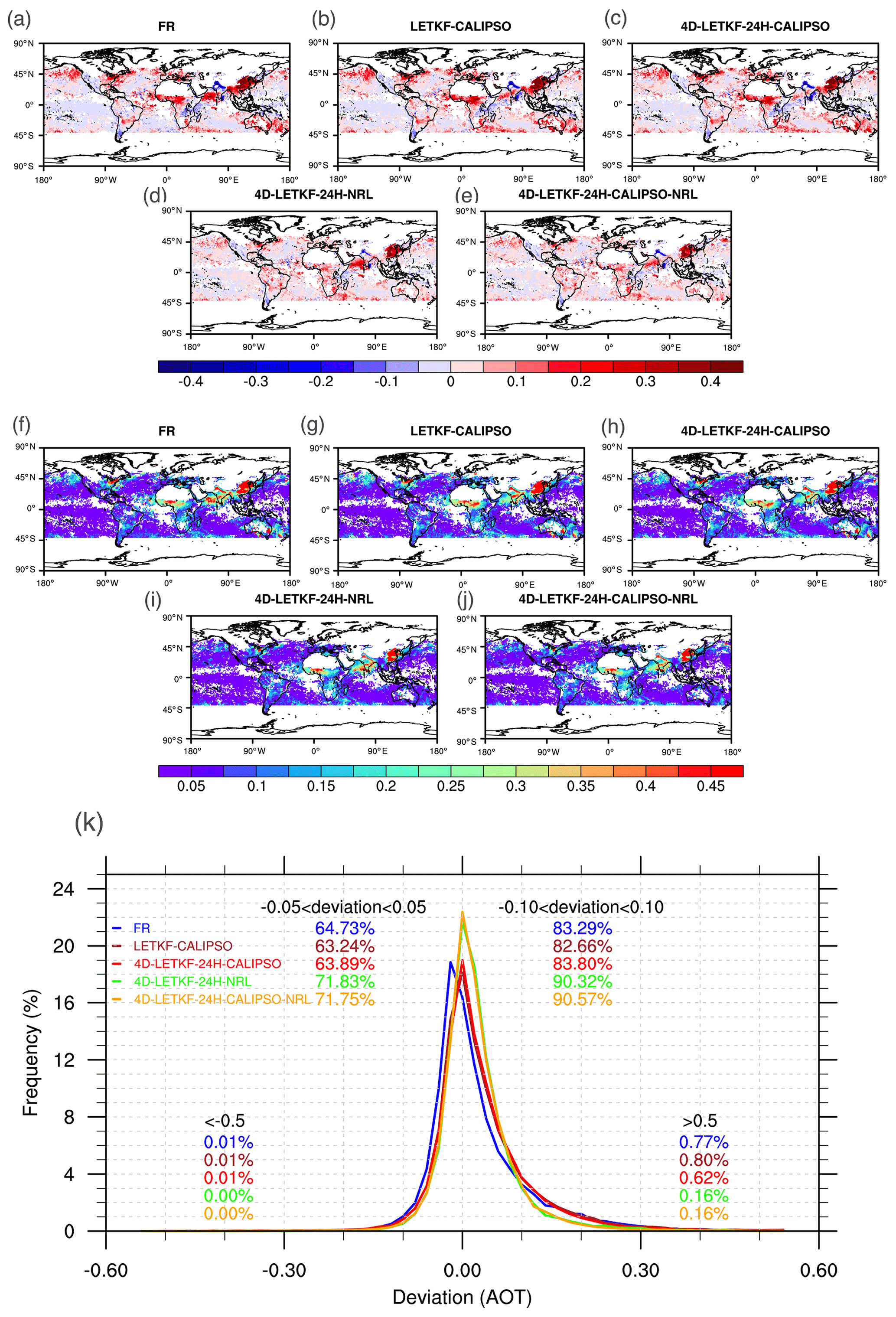
Figure 8Spatial distributions of the biases (the simulated AOTs minus the observed ones) (a, b, c, d, e) and root mean square errors (f, g, h, i, j) between the simulated and Naval Research Laboratory (NRL) Moderate Resolution Imaging Spectroradiometer (MODIS) AOTs at 550 nm during November 2016 for the FR, LETKF-CALIPSO, 4D-LETKF-24H-CALIPSO, 4D-LETKF-24H-NRL, and 4D-LETKF-24H-CALIPSO-NRL experiments. (k) Frequency distributions of deviations (the simulated AOTs minus the observed ones) from the NRL MODIS observations. The percentages of deviations between ±0.05, ±0.10, , and >0.5 are also shown.
4.2 Independent validation of the analysis with AERONET AOTs
As shown in Fig. 9a–j, we further present maps of statistical metrics (biases and RMSEs) between the modeled and AERONET-observed AOTs at 440 nm calculated over the whole month at each AERONET station as an independent validation for the five experiments. We select an AERONET site if it simultaneously has at least 10 h in 1 month (not necessarily consecutive) during which the hourly AOTs are not missing. In order to make the statistics significant, we require at least 10 observations at each selected site. A total of 191 AERONET sites are selected for comparison. Due to the sparse CALIOP observations and the localization used in the assimilation system, the simulated AOTs in many model grids are unable to be affected by the aerosol data assimilation. Therefore, we only analyze the simulated AOTs with more than 30 % variation between the 4D-LETKF-24H-CALIPSO and FR experiments hereafter. The bias in the FR experiment indicates that the model tends to underestimate AOTs over 60 % of stations in the world but overestimate AOTs over polluted industrial regions such as eastern America, western Europe, and South and East Asia. The strongest biases and highest RMSEs in the FR experiment are both found in South and East Asia, and this is due to large uncertainties in the temporal and spatial distributions of the anthropogenic aerosol emissions. The four assimilation experiments, especially the experiments including MODIS observations, clearly reduce the biases and RMSEs over regions such as eastern America and western Europe. The 4D-LETKF-24H-NRL experiment decreases the bias and RMSE over 140 (73 %) and 153 (80 %) of the total available 191 AERONET sites, respectively. The LETKF-CALIPSO and 4D-LETKF-24H-CALIPSO experiments decrease the biases at 58 % and 63 % of sites, respectively. This indicates that the CALIOP assimilation using the 4-D LETKF method is slightly superior to the one using the LETKF method. We also give PDF plots of the AOT deviations between the simulated hourly AOTs and the AERONET-observed ones for the five experiments. The negatively biased PDF for the FR experiment also reveals that the simulated AOTs are underestimated globally. The biases are improved as the peaks near 0 with both the CALIOP and MODIS assimilations, and the performance of the two assimilation experiments including MODIS observations are better than the two experiments with only CALIOP assimilation. The frequency of AOT deviations within ±0.05 (±0.10) increases from 46.25 % (65.96 %) in the FR experiment to 57.89 % (75.90 %) in the 4D-LETKF-24H-NRL experiment and 57.35 % (76.38 %) in the 4D-LETKF-24H-CALIPSO-NRL experiment. This indicates that the inclusion of the CALIOP data has an insignificant impact on the AOT analysis, which is also mentioned in Zhang et al. (2014). This is because the MODIS observations include more aerosol column information than the CALIOP observations.

Figure 9Same as Fig. 8 but for the simulated AOTs at 440 nm against the AERONET-retrieved ones.
Figure 10a shows detailed comparisons of the temporal evolutions of the hourly AOTs at 440 nm for the five experiments with the AERONET-retrieved ones over the site called Pushan_NU. Compared to the simulated AOTs in the FR experiment, the modeled AOTs in the assimilation experiments are much closer to the AERONET-observed ones, especially in terms of reducing the significant overestimations of AOTs from 3 to 7 November. The overestimations in the FR experiment are mainly induced by sulfate production due to aqueous-phase conversion from SO2. The CALIOP-derived vertical aerosol subtypes (Fig. 10m) are dominated by sea salt and other aerosols, proving that the simulated sulfate production in the FR experiment is incorrect. In fact, there are no CALIOP orbit paths that pass the Pushan_NU site, indicating that the improvements of the AOTs over 3 to 7 November can benefit from the assimilation of the CALIOP aerosol extinctions near the Pushan_NU site. Figure 10b shows the vertical distributions of the aerosol extinctions at 532 nm over one CALIOP orbit path near the Pushan_NU site at around 18:00 UTC on 3 November, and Fig. 10d, f, h, j, and l show the corresponding simulated ones of the five experiments. It is apparent that the FR experiment tends to overestimate the aerosol extinctions with the centers located at altitudes of 1–2 km from 33∘ N and 124∘ E to 38∘ N and 126∘ E, while the experiments with CALIOP assimilation, especially the 4D-LETKF-24H-CALIPSO experiment rather than the 4D-LETKF-24H-NRL experiment, correctly eliminates the unrealistically high extinction coefficients, making both the aerosol extinctions and AOTs more in accordance with the CALIOP and AERONET observations. This indicates that CALIOP assimilation is superior to MODIS assimilation in the optimization of the aerosol vertical distribution, although the MODIS assimilation can better improve the aerosol total column properties.
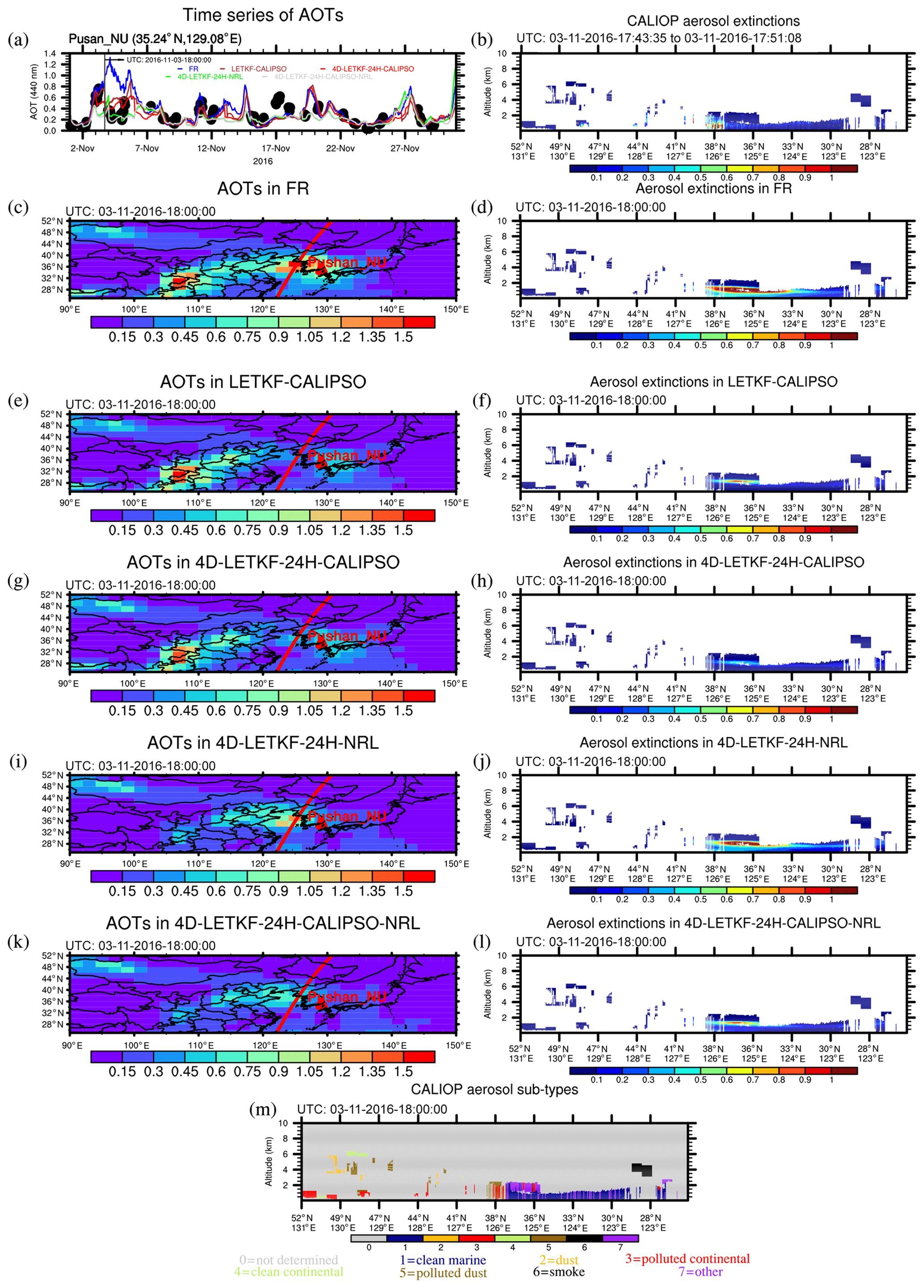
Figure 10(a) Hourly time series of the AOTs at 440 nm for the FR, LETKF-CALIPSO, 4D-LETKF-24H-CALIPSO, 4D-LETKF-24H-NRL, and 4D-LETKF-24H-CALIPSO-NRL experiments and the observed AOTs from the AErosol RObotic NETwork (AERONET) over the Pushan_NU site during November 2016. The root mean square error (RMSE) and correlation coefficient (CORR) between the simulated and observed AOTs are also shown. The spatial distributions of the simulated AOTs at 440 nm at 18:00:00 (UTC) on 3 November 2016 in the FR (c), LETKF-CALIPSO (e), 4D-LETKF-24H-CALIPSO (g), 4D-LETKF-24H-NRL (i), and 4D-LETKF-24H-CALIPSO-NRL (k) experiments. The red triangle indicates the location of the Pushan_NU site. The red curve indicates one CALIPSO orbit path near the Pushan_NU site on 3 November 2016. The CALIOP-observed aerosol extinction coefficients at 532 nm (km−1) (b) and the simulated ones at 550 nm in the FR (d), LETKF-CALIPSO (f), 4D-LETKF-24H-CALIPSO (h), 4D-LETKF-24H-NRL (j), and 4D-LETKF-24H-CALIPSO-NRL (l) experiments over that CALIPSO orbit path. (m) CALIPSO-derived vertical aerosol subtypes.
4.3 Independent validation of the analysis with independent MODIS Aqua AOTs
In order to perform an independent validation with the MODIS Aqua AOT products, we screen out the portions of the MODIS Aqua AOT products that are the same as the assimilated NRL MODIS dataset. As shown in Fig. 11a–j, we give the spatial distributions of the biases and RMSEs between the simulated and independent MODIS Aqua-observed AOTs at 550 nm for the five experiments. The AOTs over ocean areas are generally underestimated in the FR experiment, and all four assimilation experiments correctly increase the sea salt aerosols, leading to lower biases and RMSEs over the ocean. It is apparent that the four assimilation experiments also improve the model performances over the tropical Atlantic located downwind of North Africa. This is mainly caused by reductions of transported dust and OC aerosols (shown in Fig. S2), indicating that both the CALIOP and MODIS assimilation improve the simulation of the characteristics of aerosol transport from Africa to the Atlantic. For eastern China and Australia, the RMSEs in the 4D-LETKF-24H-CALIPSO experiment are obviously lower than the ones in the LETKF-CALIPSO experiment.

Figure 11Same as Fig. 8 but for the simulated AOTs at 550 nm against the independent MODIS Aqua ones.
Interestingly, it is found that the AOTs in the experiments with CALIOP assimilation have larger biases and RMSEs with the MODIS Aqua AOTs over the western part of the Sahara compared to the FR experiment, whereas such a discrepancy is not found between the FR and 4D-LETKF-24H-NRL experiments. The CALIOP (MODIS) assimilation reduces (increases) dust AOTs over the western part of the Sahara. To investigate the possible reason, Fig. 12 gives the spatial distributions of the multi-annual mean AOTs at 550 nm for MODIS Aqua, daytime CALIOP, and nighttime CALIOP at 532 nm. The CALIOP AOTs are significantly lower than the MODIS AOTs over the western Saharan region, indicating that the larger discrepancy of AOT comparisons with MODIS by the CALIOP assimilation is probably due to the differences between the CALIOP and MODIS observations in this region. Ma et al. (2013) also mentioned that the CALIPSO AOT is significantly lower than the MODIS AOT over dust regions, especially over the Saharan region. Schuster et al. (2012) found that the relative and absolute biases are probably due to the assumed lidar ratio for the CALIPSO dust retrieval being too low. We also show PDF plots of the AOT deviations between the simulated hourly AOTs and the independent MODIS Aqua-observed ones for the five experiments. Similar to the comparison with AERONET AOTs, the frequencies of AOT deviations within ±0.05 (±0.10) in 4D-LETKF-24H-CALIPSO are slightly higher than the ones in the LETKF-CALIPSO experiment. Moreover, the shape of the PDF plots in 4D-LETKF-24H-NRL and 4D-LETKF-24H-CALIPSO-NRL are similar, except the peak of the experiment with multi-sensor assimilation is a bit lower than the other one.
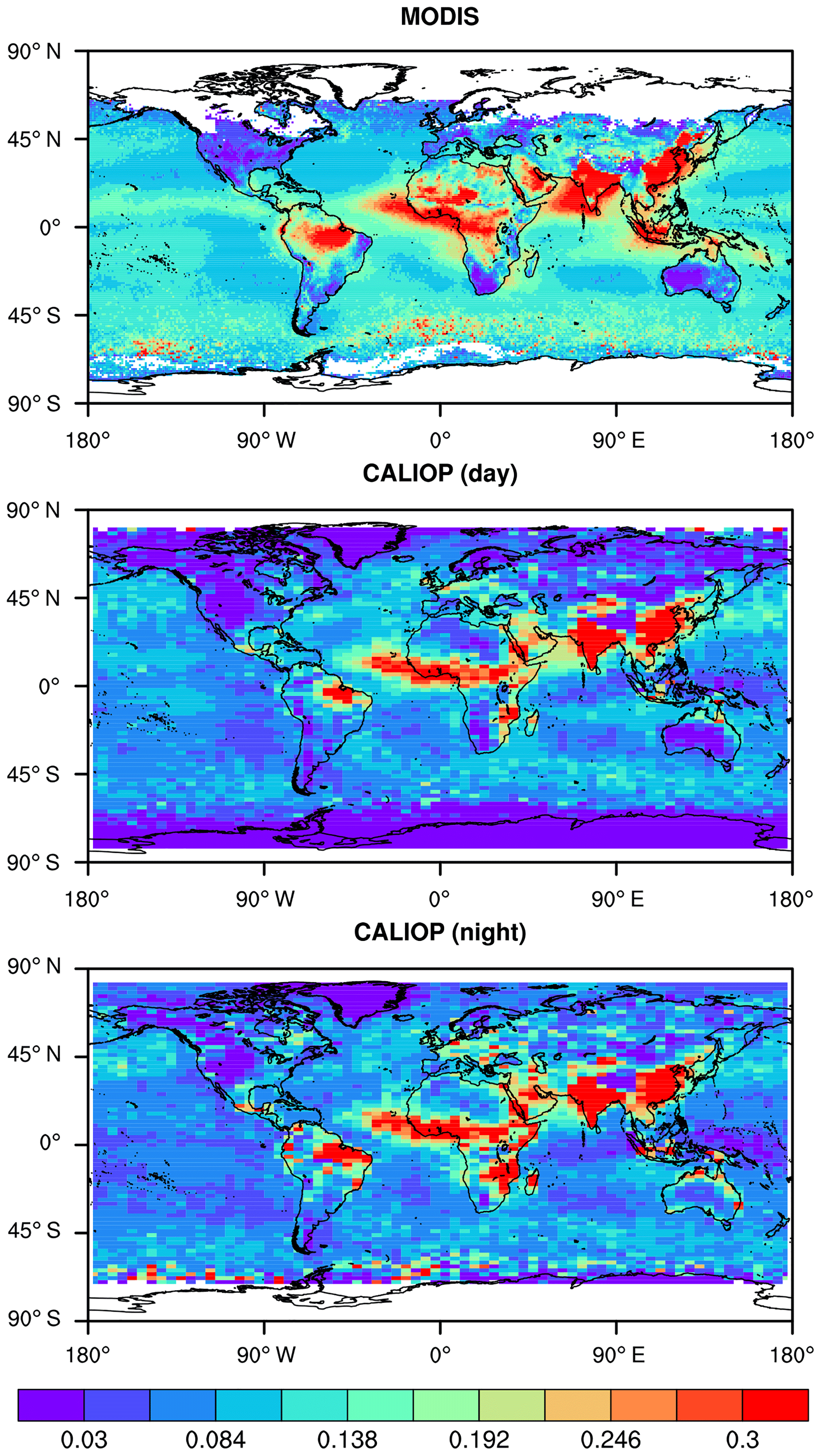
Figure 12Spatial distributions of the monthly mean MODIS Aqua AOTs at 550 nm, as well as daytime CALIOP and nighttime CALIOP AOTs at 532 nm in November from 2006 to 2016.
4.4 Independent validation of the analysis with independent CALIOP aerosol extinctions
To perform an independent validation of the aerosol vertical distribution, we conduct three other assimilation experiments like the LETKF-CALIPSO, 4D-LETKF-24H-CALIPSO, and 4D-LETKF-24H-CALIPSO-NRL experiments except only assimilating the CALIOP observations in the nighttime (hereafter called LETKF-CALIPSO-night, 4D-LETKF-24H-CALIPSO-night, and 4D-LETKF-24H-CALIPSO-NRL-night), and then we use the remaining CALIOP observations in the daytime for independent validation. Since the CALIOP observations over land in the daytime are very limited (shown in Fig. S3), we only show the results over the global ocean. Figure 13a–e show scatter plots of the daytime CALIOP extinctions versus the simulated ones in the five experiments. It is found that all assimilation experiments improve the model performance of the simulated aerosol vertical distribution. With respect to the CALIOP assimilation, the 4-D LETKF method is obviously superior to the LETKF. This is because the analyses are the same as the forecast results during the time slots when there are no CALIOP extinction observations to be assimilated in the LETKF experiment, since the LETKF only optimizes the aerosol fields when CALIOP extinction observations are available and provide the initial conditions for the next forward simulation. However, 4-D LETKF can optimize the aerosol fields over all the time slots in the assimilation window by assimilating asynchronous observations. The 4-D LETKF CALIOP assimilation is better than the MODIS assimilation, indicating that the optimized aerosol vertical distributions benefit more from the CALIOP vertical observations than the MODIS column-integrated observations. Based on the statistical metrics, the 4D-LETKF-24H-CALIPSO-NRL-night experiment has the best performance among the four assimilation experiments. This is probably due to the fact that the aerosol vertical distributions, which are unable to be optimized by assimilating the sparse CALIOP observations, are further optimized by the MODIS observations. The PDF plots in Fig. 13f further prove that the aerosol vertical observations are critical for constraining the aerosol vertical simulation, and the simultaneous assimilation of CALIOP and MODIS observations has the best performance. It is obvious that the aerosol extinctions in the daytime are underestimated in the FR experiment over the global ocean, whereas the underestimation is improved by both MODIS and CALIOP assimilations, and the peak is nearer to 0. Merely 11.31 % (24.84 %) of the extinction deviations in the FR experiment are within ±0.01(±0.02), whereas 35.01 % (57.95 %) of the extinction deviations in the 4D-LETKF-24H-CALIPSO-NRL-night experiment are within ±0.01(±0.02).
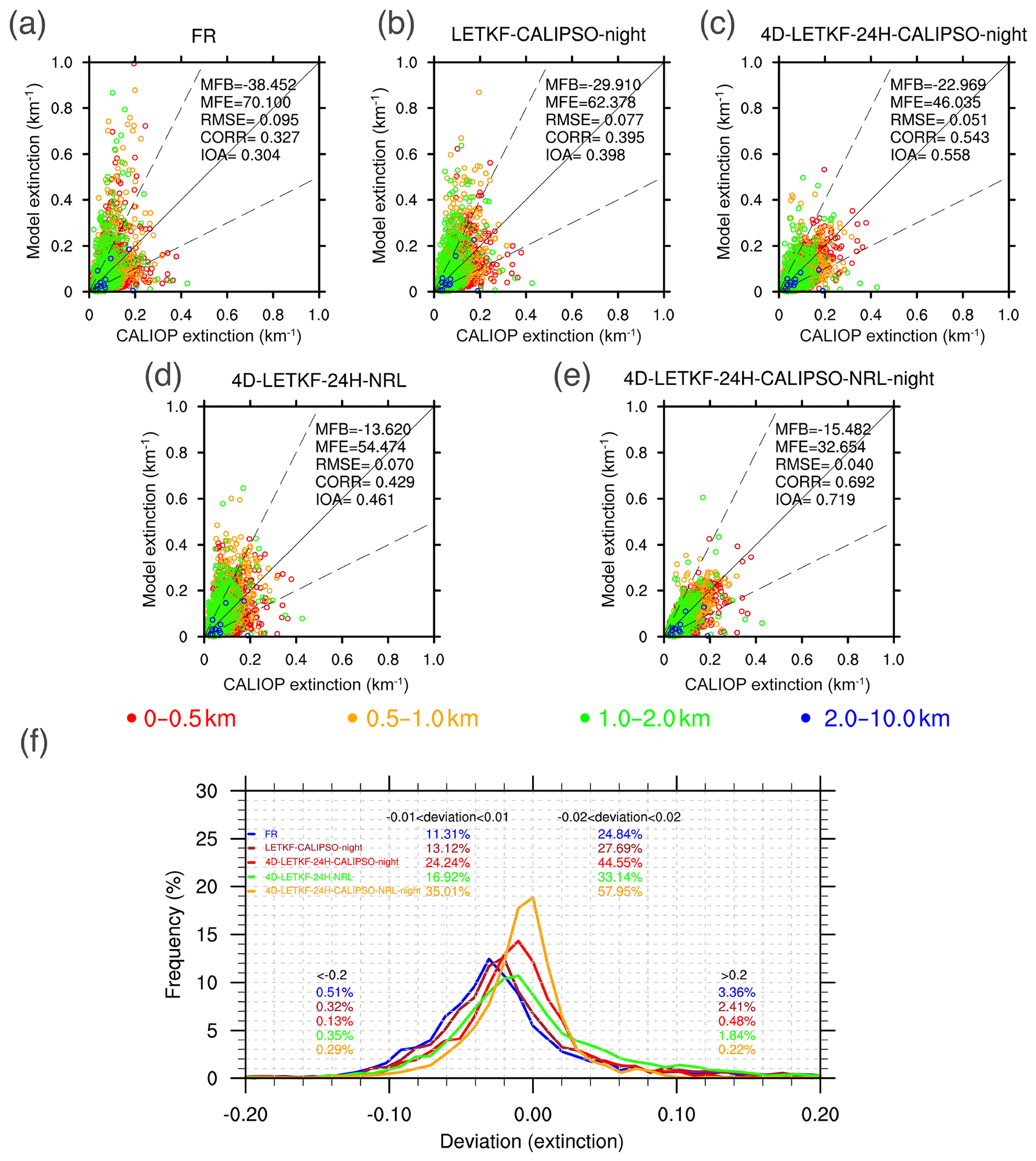
Figure 13Scatter plots of the simulated hourly aerosol extinction coefficients in the daytime at 550 nm (km−1) for the FR (a), LETKF-CALIPSO-night (b), 4D-LETKF-24H-CALIPSO-night (c), 4D-LETKF-24H-NRL (d), and 4D-LETKF-24H-CALIPSO-NRL-night (e) experiments versus the CALIOP-observed ones in the daytime at 532 nm. (f) Frequency distributions of deviations (modeled extinction coefficients minus the CALIOP-observed ones in the daytime). The percentages of deviations between ±0.01, ±0.02, , and >0.2 are also shown.
As shown in Fig. 14, we also give the mean vertical profiles of the CALIOP-observed and model-simulated aerosol extinction coefficients over the global ocean in the daytime. We ignore the levels above 2 km since there are limited CALIOP observations. It is apparent that there are significant discrepancies between the FR experiment and the CALIOP observation. Both the CALIPSO assimilation with LETKF and the MODIS assimilation have limited improvements of the simulated aerosol extinction profiles. With respect to the 4D-LETKF-24H-CALIPSO-night and the 4D-LETKF-24H-CALIPSO-NRL-night experiments, the aerosol profiles below 0.6 km are generally consistent with the independent CALIOP observations, and the aerosol profiles from 0.6 to 1.2 km are more comparable to the observed one than those of the other experiments. The discrepancies of the aerosol extinction profiles between the 4D-LETKF-24H-CALIPSO-night and 4D-LETKF-24H-CALIPSO-NRL-night experiments are obvious above 1 km. This is because there are fewer CALIOP observations over 1 km, and this induces the NRL MODIS AOTs to play a more important role in modifying the profile.
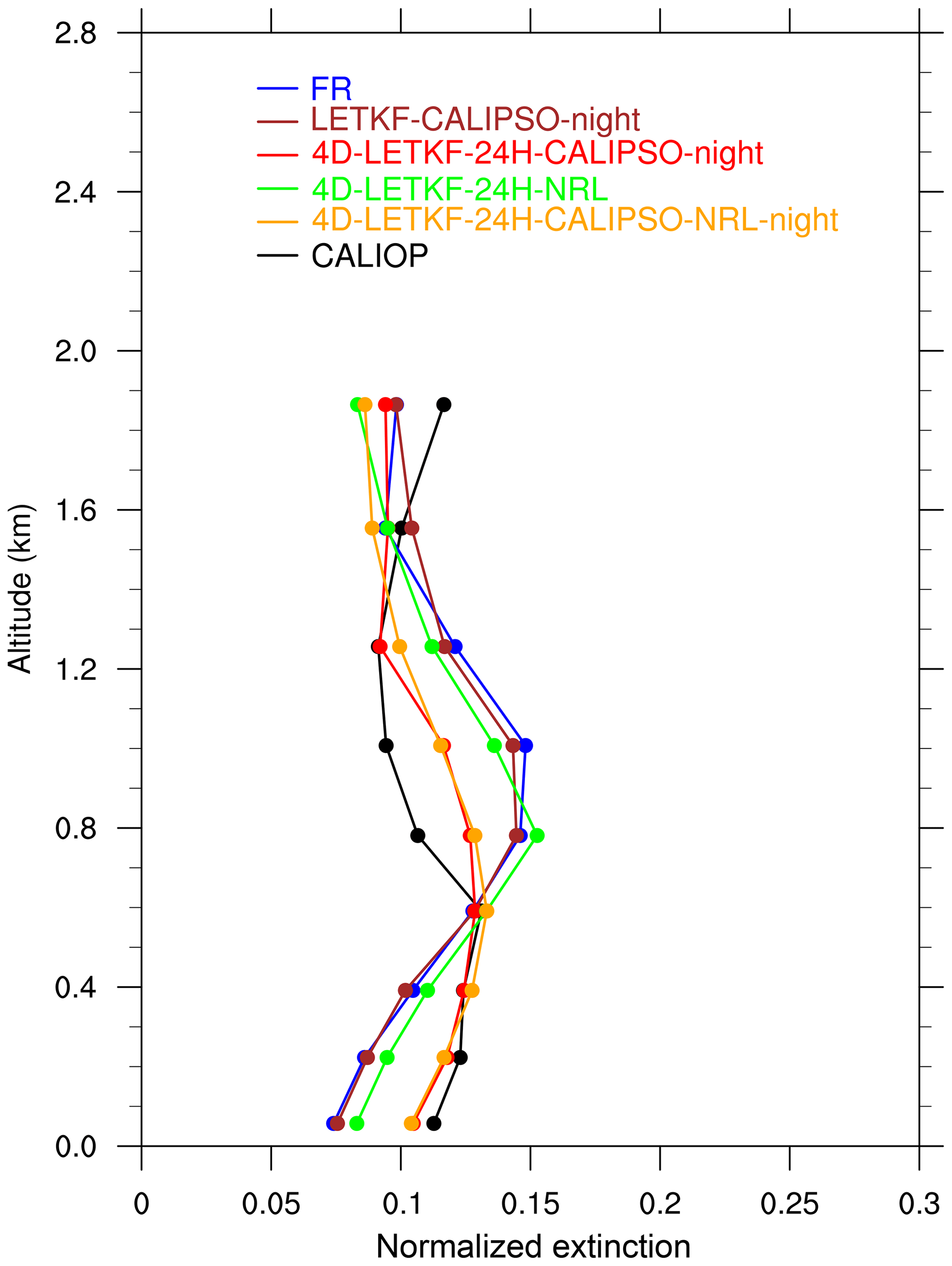
Figure 14Averaged monthly mean vertical profiles of the simulated normalized aerosol extinction coefficients in the daytime at 550 nm (km−1) in the five experiments and the CALIOP-observed ones in the daytime at 532 nm.
From our results so far, both the CALIOP and MODIS assimilation can improve the magnitude of the simulated aerosol extinctions; however, the CALIOP assimilation is superior to the MODIS assimilation in terms of modifying the incorrect aerosol vertical distributions and reproducing the real magnitudes and variations. The simultaneous assimilation of the CALIOP and MODIS observations is better than separate assimilation in reproducing aerosol vertical information.
CALIPSO provides sparse observations due to sensor-specific data gaps for a 16 d repeat cycle. To investigate the effects of CALIPSO sensor gaps on the data assimilation, Fig. 15 shows the assimilation efficiencies (AEs), referred to in Yumimoto and Takemura (2011), with the MODIS Aqua-observed AOTs as a function of the CALIOP overpass time. The hourly and daily mean AEs both show decreasing trends with increasing distance from the assimilation time. The AEs are high close to the overpass time but deteriorate later on. Such a deterioration demonstrates that more intensive vertical observations can improve the aerosol vertical assimilation efficiency and hence advance the study of aerosol effects on the climate and environment.

Figure 15Assimilation efficiencies (AEs) calculated against the Moderate Resolution Imaging Spectroradiometer (MODIS) Aqua-observed AOTs at 550 nm for the 4D-LETKF-24H-CALIPSO experiment as a function of the distance from the assimilation time. The daily mean time series and the linear regression line are shown as the blue solid and black dashed lines, respectively.
To investigate the effects of the assimilation system parameters (i.e., horizontal localization length, vertical localization length, and uncertainty of dust emissions) for the CALIOP and MODIS assimilation in this study, five other assimilation experiments called 4D-LETKF-24H-CALIPSO-HL500, 4D-LETKF-24H-CALIPSO-HL1000, 4D-LETKF-24H-CALIPSO-HL2000, 4D-LETKF-24H-CALIPSO-VL, and 4D-LETKF-24H-CALIPSO-Dust are conducted. The experiments are in the same model configuration as that of the 4D-LETKF-24H-CALIPSO experiment except for the following: horizontal localization lengths of 500, 1000, and 2000 km are used in the 4D-LETKF-24H-CALIPSO-HL500, 4D-LETKF-24H-CALIPSO-HL1000, and 4D-LETKF-24H-CALIPSO-HL2000 experiments; 4 times the vertical localization length is used in the 4D-LETKF-24H-CALIPSO-VL experiment; and 5 times the assumed dust uncertainty is used in the 4D-LETKF-24H-CALIPSO-Dust experiment. Figure 16 shows the frequencies of the AOT deviations between the simulations of the six CALIOP assimilation experiments and the independent MODIS observations. In addition, the corresponding result of the FR experiment is also shown as a reference. Among the six assimilation experiments, the 4D-LETKF-24H-CALIPSO experiment shows the highest percentage of deviation between ±0.05 and ±0.10. By the increments of the horizontal localization length, the percentage of deviation between ±0.05 and ±0.10 decreases and the peaks of the PDF plots tend far away from 0. The significant differences between the 4D-LETKF-24H-CALIPSO and 4D-LETKF-24H-CALIPSO-VL experiments indicate that one model layer is a reasonable vertical localization length and a larger one will reduce the assimilation ability. Therefore, we use the 200 km horizontal localization length (i.e., observations located within 730 km are assimilated), one model layer vertical localization length, and 100 % dust perturbation assuming uncertainties for the aerosol data assimilation in this study.
The assimilation of aerosol vertical observations can provide more accurate spatiotemporal distributions of aerosol characteristics, especially vertical information, which should advance studies of aerosol effects on the Earth system. In the present study, we develop the 4-D LETKF assimilation system for the CALIOP vertical extinction observations and successfully present a 1-month-long hourly aerosol analysis during November 2016. The hourly analyses are compared with the assimilated observations as internal checks and validated by independent AERONET-retrieved AOTs, MODIS Aqua AOTs, and daytime CALIOP extinctions. The effects of assimilating the observations by including the vertical information (or not) and the impacts of the multi-sensor assimilation on the model performances are also investigated.
Compared with the assimilated CALIOP observations as internal checks, the two CALIOP assimilation experiments are evidently better than the FR experiment, especially over the ocean regions. Compared with the assimilated NRL MODIS AOTs, the 4D-LETKF-24H-NRL experiment is superior to the FR experiment as indicated by the reduced biases. These results indicate that the assimilation system is operated successfully. The performances of the 4D-LETKF-24H-CALIPSO experiment are generally comparable to those of the LETKF-CALIPSO experiment. This indicates that the weights determined at the end of the 24 h assimilation window are valid to optimize the ensemble trajectories, and the temporally remote asynchronous observations within 24 h have a limited influence on the analysis. Moreover, the elapsed time for the 1-month assimilation over November 2016 with 4D-LETKF-24H-CALIPSO is much shorter than that of the LETKF-CALIPSO experiment. This is due to 4-D LETKF avoiding frequent switching between the assimilation and model ensemble forecasts.
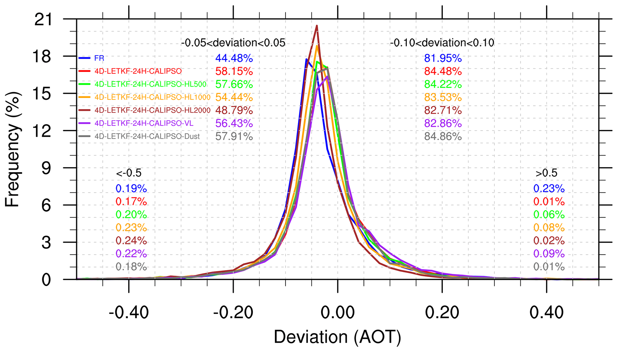
Figure 16Frequency distributions of deviations (the simulated AOTs minus the observed AOTs) from the Moderate Resolution Imaging Spectroradiometer (MODIS) Aqua-observed AOTs at 550 nm for the FR, 4D-LETKF-24H-CALIPSO, 4D-LETKF-24H-CALIPSO-L500, 4D-LETKF-24H-CALIPSO-L1000, 4D-LETKF-24H-CALIPSO-L2000, 4D-LETKF-24H-CALIPSO-VL, and 4D-LETKF-24H-CALIPSO-Dust experiments. The percentages of deviations between ±0.05, ±0.10, , and >0.5 are also shown.
Compared with the independent MODIS- and AERONET-retrieved AOTs, CALIOP and MODIS assimilation can both achieve improved model-simulated AOTs over most land and ocean regions. However, the experiments with MODIS assimilation can reproduce better agreement with the independent AERONET AOTs than the experiments only assimilating CALIOP observations. This is probably due to CALIOP (with a 16 d repeat cycle) having much sparser coverage than MODIS and the assimilation efficiencies of CALIOP decreasing with increasing distance from the assimilation time. Compared with the individual MODIS assimilation, the inclusion of CALIOP observations has an insignificant impact on the AOT analysis. This is because the MODIS observations include more aerosol column information than the CALIOP observations.
With assimilating the nighttime CALIOP observations and using the remaining CALIOP observations in the daytime for independent validation, it is found that both CALIOP and MODIS assimilation can improve the magnitude of the simulated aerosol extinctions; however, the CALIOP assimilation is superior to the MODIS assimilation in terms of modifying incorrect aerosol vertical distributions and reproducing the real magnitudes and variations. Compared with the independent CALIOP extinction observations in the daytime over the ocean, the 4-D LETKF CALIOP assimilation is better than the MODIS assimilation. This indicates that the optimized aerosol vertical distributions benefit more from the CALIOP vertical observations than the MODIS column-integrated observations. The simultaneous CALIOP and MODIS assimilation experiment has the best performance. This is probably due to the fact that the aerosol vertical distributions, which are unable to be optimized by assimilating the sparse CALIOP observations, are further optimized by the MODIS observations.
The assimilation of the CALIOP extinction observations deteriorates the model performance over the western part of the Sahara compared to the MODIS observations. This is due to the inconsistences between the CALIOP and MODIS observations, indicating that the assumed lidar ratio, which is important for aerosol extinction retrieval, still has uncertainties, especially in dust regions, and the data quality needs to be improved to advance model skill over these regions.
The assimilation efficiencies are high close to the overpass time but deteriorate later on. This indicates that more aerosol vertical observation platforms are required to fill sensor-specific observation gaps for better aerosol vertical data assimilation. In the near future, joint assimilation of aerosol profile observations from the Earth Cloud Aerosol and Radiation Explorer (EarthCARE) and CALIPSO may further advance our understanding of atmospheric aerosol vertical characteristics.
The data and data analysis methods are available upon request. The NICAM source code is available with terms and conditions at http://nicam.jp/hiki/?Research+Collaborations (last access: 15 September 2019; Satoh et al., 2014).
The supplement related to this article is available online at: https://doi.org/10.5194/acp-19-13445-2019-supplement.
TD designed the experiments. YC carried out the experiments and conducted the data analysis with contributions from all coauthors. YC prepared the paper with help from TD, DG, NAJS, GS, and TN.
The authors declare that they have no conflict of interest.
The model simulations were performed using the supercomputer resources NIES/NEC SX-ACE and JAXA/JSS2. We are grateful to the relevant researchers who provided the observation data from AERONET (http://www.eorc.jaxa.jp/ptree/index.html, last access: 15 September 2019) and MODIS (https://modis-atmos.gsfc.nasa.gov/products/aerosol, last access: 15 September 2019). CALIPSO data were obtained from the NASA Langley Research Center–Atmospheric Sciences Data Center (ASDC). We also thank two anonymous reviewers for their insightful comments and suggestions.
This research has been supported by the Strategic Priority Research Program of the Chinese Academy of Sciences (grant no. XDA2006010302), the National Key R&D Program of China (grant nos. 2016YFC0202001 and 2017YFC0209803), and the National Natural Science Funds of China (grant nos. 41571130024, 41605083, 41590875, and 41475031). Some of the authors are supported by the Global Environment Research and Technology Development Fund S-12 of MOEJ, the Japan Aerospace Exploration Agency (JAXA)/Earth Observation Priority Research and the JSPS KAKENHI (grant nos. 17H04711 and 19H05669) in Japan.
This paper was edited by Jianping Huang and reviewed by three anonymous referees.
Benedetti, A., Morcrette, J.-J., Boucher, O., Dethof, A., Engelen, R. J., Fisher, M., Flentje, H., Huneeus, N., Jones, L., Kaiser, J. W., Kinne, S., Mangold, A., Razinger, M., Simmons, A. J., and Suttie, M.: Aerosol analysis and forecast in the European Centre for Medium-Range Weather Forecasts Integrated Forecast System: 2. Data assimilation, J. Geophys. Res., 114, D13205, https://doi.org/10.1029/2008JD011115, 2009.
Boylan, J. W. and Russell, A. G.: PM and light extinction model performance metrics, goals, and criteria for three-dimensional air quality models, Atmos. Environ., 40, 4946–4959, https://doi.org/10.1016/j.atmosenv.2005.09.087, 2006.
Charlson, R. J., Schwartz, S. E., Hales, J. M., Cess, R. D., Coakley, J. A., Hansen, E., and Hofmann, D. J.: Climate Forcing by Anthropogenic Aerosols, Science, 255, 423–430, 1992.
Dai, T., Schutgens, N. A. J., Goto, D., Shi, G., and Nakajima, T.: Improvement of aerosol optical properties modeling over Eastern Asia with MODIS AOD assimilation in a global non-hydrostatic icosahedral aerosol transport model, Environ. Pollut., 195, 319–329, https://doi.org/10.1016/j.envpol.2014.06.021, 2014a.
Dai, T., Goto, D., Schutgens, N. A. J., Dong, X., Shi, G., and Nakajima, T.: Simulated aerosol key optical properties over global scale using an aerosol transport model coupled with a new type of dynamic core, Atmos. Environ., 82, 71–82, https://doi.org/10.1016/j.atmosenv.2013.10.018, 2014b.
Dai, T., Cheng, Y., Zhang, P., Shi, G., Sekiguchi, M., Suzuki, K., Goto, D., and Nakajima, T.: Impacts of meteorological nudging on the global dust cycle simulated by NICAM coupled with an aerosol model, Atmos. Environ., 190, 99–115, https://doi.org/10.1016/j.atmosenv.2018.07.016, 2018.
Dai, T., Cheng, Y., Suzuki, K., Goto, D., Kikuchi, M., Schutgens, N. A. J., Yoshida, M., Zhang, P., Husi, L., Shi, G., and Nakajima, T.: Hourly Aerosol Assimilation of Himawari-8 AOT Using the Four-Dimensional Local Ensemble Transform Kalman Filter, J. Adv. Model. Earth Syst., 11, 680–711, https://doi.org/10.1029/2018MS001475, 2019.
Di Tomaso, E., Schutgens, N. A. J., Jorba, O., and Pérez García-Pando, C.: Assimilation of MODIS Dark Target and Deep Blue observations in the dust aerosol component of NMMB-MONARCH version 1.0, Geosci. Model Dev., 10, 1107–1129, https://doi.org/10.5194/gmd-10-1107-2017, 2017.
Evensen, G.: Sequential data assimilation with a nonlinear quasi-geostrophic model using Monte Carlo methods to forecast error statistics, J. Geophys. Res., 99, 10143, https://doi.org/10.1029/94JC00572, 1994.
Gaspari, G. and Cohn, S. E.: Construction of correlation functions in two and three dimensions, Q. J. Roy. Meteorol. Soc., 125, 723–757, https://doi.org/10.1002/qj.49712555417, 1999.
Generoso, S., Bréon, F.-M., Chevallier, F., Balkanski, Y., Schulz, M., and Bey, I.: Assimilation of POLDER aerosol optical thickness into the LMDz-INCA model: Implications for the Arctic aerosol burden, J. Geophys. Res., 112, D02311, https://doi.org/10.1029/2005JD006954, 2007.
Giles, D. M., Sinyuk, A., Sorokin, M. G., Schafer, J. S., Smirnov, A., Slutsker, I., Eck, T. F., Holben, B. N., Lewis, J. R., Campbell, J. R., Welton, E. J., Korkin, S. V., and Lyapustin, A. I.: Advancements in the Aerosol Robotic Network (AERONET) Version 3 database – automated near-real-time quality control algorithm with improved cloud screening for Sun photometer aerosol optical depth (AOD) measurements, Atmos. Meas. Tech., 12, 169–209, https://doi.org/10.5194/amt-12-169-2019, 2019.
Ginoux, P., Chin, M., Tegen, I., Prospero, J. M., Holben, B., Dubovik, O., and Lin, S.-J.: Sources and distributions of dust aerosols simulated with the GOCART model, J. Geophys. Res.-Atmos., 106, 20255–20273, https://doi.org/10.1029/2000JD000053, 2001.
Goto, D., Dai, T., Satoh, M., Tomita, H., Uchida, J., Misawa, S., Inoue, T., Tsuruta, H., Ueda, K., Ng, C. F. S., Takami, A., Sugimoto, N., Shimizu, A., Ohara, T., and Nakajima, T.: Application of a global nonhydrostatic model with a stretched-grid system to regional aerosol simulations around Japan, Geosci. Model Dev., 8, 235–259, https://doi.org/10.5194/gmd-8-235-2015, 2015.
Grythe, H., Ström, J., Krejci, R., Quinn, P., and Stohl, A.: A review of sea-spray aerosol source functions using a large global set of sea salt aerosol concentration measurements, Atmos. Chem. Phys., 14, 1277–1297, https://doi.org/10.5194/acp-14-1277-2014, 2014.
Holben, B. N., Eck, T. F., Slutsker, I., Tanré, D., Buis, J. P., Setzer, A., Vermote, E., Reagan, J. A., Kaufman, Y. J., Nakajima, T., Lavenu, F., Jankowiak, I., and Smirnov, A.: AERONET – A Federated Instrument Network and Data Archive for Aerosol Characterization, Remote Sens. Environ., 66, 1–16, https://doi.org/10.1016/S0034-4257(98)00031-5, 1998.
Huang, J., Minnis, P., Yi, Y., Tang, Q., Wang, X., Hu, Y., Liu, Z., Ayers, K., Trepte, C., and Winker, D.: Summer dust aerosols detected from CALIPSO over the Tibetan Plateau, Geophys. Res. Lett., 34, L18805, https://doi.org/10.1029/2007GL029938, 2007.
Huang, J., Fu, Q., Su, J., Tang, Q., Minnis, P., Hu, Y., Yi, Y., and Zhao, Q.: Taklimakan dust aerosol radiative heating derived from CALIPSO observations using the Fu-Liou radiation model with CERES constraints, Atmos. Chem. Phys., 9, 4011–4021, https://doi.org/10.5194/acp-9-4011-2009, 2009.
Huang, J. P., Liu, J. J., Chen, B., and Nasiri, S. L.: Detection of anthropogenic dust using CALIPSO lidar measurements, Atmos. Chem. Phys., 15, 11653–11665, https://doi.org/10.5194/acp-15-11653-2015, 2015.
Huang, J., Yu, H., Dai, A., Wei, Y., and Kang, L.: Drylands face potential threat under 2 ∘ C global warming target, Nat. Clim. Change, 7, 417–422, https://doi.org/10.1038/nclimate3275, 2017.
Huang, L., Jiang, J. H., Tackett, J. L., Su, H., and Fu, R.: Seasonal and diurnal variations of aerosol extinction profile and type distribution from CALIPSO 5-year observations, J. Geophys. Res.-Atmos., 118, 4572–4596, https://doi.org/10.1002/jgrd.50407, 2013.
Huang, R.-J., Zhang, Y., Bozzetti, C., Ho, K.-F., Cao, J.-J., Han, Y., Daellenbach, K. R., Slowik, J. G., Platt, S. M., Canonaco, F., Zotter, P., Wolf, R., Pieber, S. M., Bruns, E. A., Crippa, M., Ciarelli, G., Piazzalunga, A., Schwikowski, M., Abbaszade, G., Schnelle-Kreis, J., Zimmermann, R., An, Z., Szidat, S., Baltensperger, U., Haddad, I. E., and Prévôt, A. S. H.: High secondary aerosol contribution to particulate pollution during haze events in China, Nature, 514, 218–222, https://doi.org/10.1038/nature13774, 2014.
Huneeus, N., Schulz, M., Balkanski, Y., Griesfeller, J., Prospero, J., Kinne, S., Bauer, S., Boucher, O., Chin, M., Dentener, F., Diehl, T., Easter, R., Fillmore, D., Ghan, S., Ginoux, P., Grini, A., Horowitz, L., Koch, D., Krol, M. C., Landing, W., Liu, X., Mahowald, N., Miller, R., Morcrette, J.-J., Myhre, G., Penner, J., Perlwitz, J., Stier, P., Takemura, T., and Zender, C. S.: Global dust model intercomparison in AeroCom phase I, Atmos. Chem. Phys., 11, 7781–7816, https://doi.org/10.5194/acp-11-7781-2011, 2011.
Hunt, B. R., Kostelich, E. J. and Szunyogh, I.: Efficient data assimilation for spatiotemporal chaos: A local ensemble transform Kalman filter, Phys. D: Nonlin. Phenom., 230, 112–126, https://doi.org/10.1016/j.physd.2006.11.008, 2007.
Hyer, E. J., Reid, J. S., and Zhang, J.: An over-land aerosol optical depth data set for data assimilation by filtering, correction, and aggregation of MODIS Collection 5 optical depth retrievals, Atmos. Meas. Tech., 4, 379–408, https://doi.org/10.5194/amt-4-379-2011, 2011.
Janssens-Maenhout, G., Crippa, M., Guizzardi, D., Dentener, F., Muntean, M., Pouliot, G., Keating, T., Zhang, Q., Kurokawa, J., Wankmüller, R., Denier van der Gon, H., Kuenen, J. J. P., Klimont, Z., Frost, G., Darras, S., Koffi, B., and Li, M.: HTAP_v2.2: a mosaic of regional and global emission grid maps for 2008 and 2010 to study hemispheric transport of air pollution, Atmos. Chem. Phys., 15, 11411–11432, https://doi.org/10.5194/acp-15-11411-2015, 2015.
Jia, R., Liu, Y., Chen, B., Zhang, Z., and Huang, J.: Source and transportation of summer dust over the Tibetan Plateau, Atmos. Environ., 123, 210–219, https://doi.org/10.1016/j.atmosenv.2015.10.038, 2015.
Kalnay, E. and Yang, S.-C.: Accelerating the spin-up of Ensemble Kalman Filtering, Q. J. Roy. Meteorol. Soc., 136, 1644–1651, https://doi.org/10.1002/qj.652, 2010.
Kittaka, C., Winker, D. M., Vaughan, M. A., Omar, A., and Remer, L. A.: Intercomparison of column aerosol optical depths from CALIPSO and MODIS-Aqua, Atmos. Meas. Tech., 4, 131–141, https://doi.org/10.5194/amt-4-131-2011, 2011.
Koffi, B., Schulz, M., Bréon, F.-M., Griesfeller, J., Winker, D., Balkanski, Y., Bauer, S., Berntsen, T., Chin, M., Collins, W. D., Dentener, F., Diehl, T., Easter, R., Ghan, S., Ginoux, P., Gong, S., Horowitz, L. W., Iversen, T., Kirkevåg, A., Koch, D., Krol, M., Myhre, G., Stier, P., and Takemura, T.: Application of the CALIOP layer product to evaluate the vertical distribution of aerosols estimated by global models: AeroCom phase I results: AEROSOL PROFILES IN GLOBAL MODELS, J. Geophys. Res.-Atmos., 117, D10201, https://doi.org/10.1029/2011JD016858, 2012.
Levy, R. C., Mattoo, S., Munchak, L. A., Remer, L. A., Sayer, A. M., Patadia, F., and Hsu, N. C.: The Collection 6 MODIS aerosol products over land and ocean, Atmos. Meas. Tech., 6, 2989–3034, https://doi.org/10.5194/amt-6-2989-2013, 2013.
Liu, Y., Huang, J., Shi, G., Takamura, T., Khatri, P., Bi, J., Shi, J., Wang, T., Wang, X., and Zhang, B.: Aerosol optical properties and radiative effect determined from sky-radiometer over Loess Plateau of Northwest China, Atmos. Chem. Phys., 11, 11455–11463, https://doi.org/10.5194/acp-11-11455-2011, 2011.
Liu, Y., Jia, R., Dai, T., Xie, Y., and Shi, G.: A review of aerosol optical properties and radiative effects, J. Meteorol. Res., 28, 1003–1028, https://doi.org/10.1007/s13351-014-4045-z, 2014.
Liu, Y., Sato, Y., Jia, R., Xie, Y., Huang, J., and Nakajima, T.: Modeling study on the transport of summer dust and anthropogenic aerosols over the Tibetan Plateau, Atmos. Chem. Phys., 15, 12581–12594, https://doi.org/10.5194/acp-15-12581-2015, 2015.
Liu, Y., Hua, S., Jia, R., and Huang, J.: Effect of Aerosols on the Ice Cloud Properties Over the Tibetan Plateau, J. Geophys. Res.-Atmos., 2019, JD030463, https://doi.org/10.1029/2019JD030463, 2019a.
Liu, Y., Zhu, Q., Huang, J., Hua, S., and Jia, R.: Impact of dust-polluted convective clouds over the Tibetan Plateau on downstream precipitation, Atmos. Environ., 209, 67–77, https://doi.org/10.1016/j.atmosenv.2019.04.001, 2019b.
Liu, Z., Liu, Q., Lin, H.-C., Schwartz, C. S., Lee, Y.-H., and Wang, T.: Three-dimensional variational assimilation of MODIS aerosol optical depth: Implementation and application to a dust storm over East Asia: AOD DATA ASSIMILATION, J. Geophys. Res.-Atmos., 116, D23206, https://doi.org/10.1029/2011JD016159, 2011.
Ma, X., Bartlett, K., Harmon, K., and Yu, F.: Comparison of AOD between CALIPSO and MODIS: significant differences over major dust and biomass burning regions, Atmos. Meas. Tech., 6, 2391–2401, https://doi.org/10.5194/amt-6-2391-2013, 2013.
Miyamoto, Y., Kajikawa, Y., Yoshida, R., Yamaura, T., Yashiro, H., and Tomita, H.: Deep moist atmospheric convection in a subkilometer global simulation: CONVECTION IN A SUB-KM GLOBAL SIMULATION, Geophys. Res. Lett., 40, 4922–4926, https://doi.org/10.1002/grl.50944, 2013.
Miyoshi, T., Yamane, S., and Enomoto, T.: Localizing the Error Covariance by Physical Distances within a Local Ensemble Transform Kalman Filter (LETKF), SOLA, 3, 89–92, https://doi.org/10.2151/sola.2007-023, 2007.
Myhre, G., Samset, B. H., Schulz, M., Balkanski, Y., Bauer, S., Berntsen, T. K., Bian, H., Bellouin, N., Chin, M., Diehl, T., Easter, R. C., Feichter, J., Ghan, S. J., Hauglustaine, D., Iversen, T., Kinne, S., Kirkevåg, A., Lamarque, J.-F., Lin, G., Liu, X., Lund, M. T., Luo, G., Ma, X., van Noije, T., Penner, J. E., Rasch, P. J., Ruiz, A., Seland, Ø., Skeie, R. B., Stier, P., Takemura, T., Tsigaridis, K., Wang, P., Wang, Z., Xu, L., Yu, H., Yu, F., Yoon, J.-H., Zhang, K., Zhang, H., and Zhou, C.: Radiative forcing of the direct aerosol effect from AeroCom Phase II simulations, Atmos. Chem. Phys., 13, 1853–1877, https://doi.org/10.5194/acp-13-1853-2013, 2013.
Nakajima, T., Higurashi, A., Kawamoto, K., and Penner, J. E.: A possible correlation between satellite-derived cloud and aerosol microphysical parameters, Geophys. Res. Lett., 28, 1171–1174, https://doi.org/10.1029/2000GL012186, 2001.
Niwa, Y., Tomita, H., Satoh, M., and Imasu, R.: A Three-Dimensional Icosahedral Grid Advection Scheme Preserving Monotonicity and Consistency with Continuity for Atmospheric Tracer Transport, J. Meteorol. Soc. JPN, 89, 255–268, https://doi.org/10.2151/jmsj.2011-306, 2011.
Oikawa, E., Nakajima, T., Inoue, T., and Winker, D.: A study of the shortwave direct aerosol forcing using ESSP/CALIPSO observation and GCM simulation: DARF USING CALIPSO AND GCM, J. Geophys. Res.-Atmos., 118, 3687–3708, https://doi.org/10.1002/jgrd.50227, 2013.
Oikawa, E., Nakajima, T., and Winker, D.: An Evaluation of the Shortwave Direct Aerosol Radiative Forcing Using CALIOP and MODIS Observations, J. Geophys. Res.-Atmos., 123, 1211–1233, https://doi.org/10.1002/2017JD027247, 2018.
Penning de Vries, M. J. M., Beirle, S., Hörmann, C., Kaiser, J. W., Stammes, P., Tilstra, L. G., Tuinder, O. N. E., and Wagner, T.: A global aerosol classification algorithm incorporating multiple satellite data sets of aerosol and trace gas abundances, Atmos. Chem. Phys., 15, 10597–10618, https://doi.org/10.5194/acp-15-10597-2015, 2015.
Ramanathan, V.: Aerosols, Climate, and the Hydrological Cycle, Science, 294, 2119–2124, https://doi.org/10.1126/science.1064034, 2001.
Remer, L. A., Kaufman, Y. J., Tanré, D., Mattoo, S., Chu, D. A., Martins, J. V., Li, R.-R., Ichoku, C., Levy, R. C., Kleidman, R. G., Eck, T. F., Vermote, E., and Holben, B. N.: The MODIS Aerosol Algorithm, Products, and Validation, J. Atmos. Sci., 62, 947–973, https://doi.org/10.1175/JAS3385.1, 2005.
Rubin, J. I., Reid, J. S., Hansen, J. A., Anderson, J. L., Holben, B. N., Xian, P., Westphal, D. L., and Zhang, J.: Assimilation of AERONET and MODIS AOT observations using variational and ensemble data assimilation methods and its impact on aerosol forecasting skill, J. Geophys. Res.-Atmos., 122, 4967–4992, https://doi.org/10.1002/2016JD026067, 2017.
Sato, Y. and Suzuki, K.: How do aerosols affect cloudiness?, Science, 363, 580–581, https://doi.org/10.1126/science.aaw3720, 2019.
Sato, Y., Goto, D., Michibata, T., Suzuki, K., Takemura, T., Tomita, H., and Nakajima, T.: Aerosol effects on cloud water amounts were successfully simulated by a global cloud-system resolving model, Nat. Commun., 9, 985, https://doi.org/10.1038/s41467-018-03379-6, 2018.
Satoh, M., Tomita, H., Miura, H., Iga, S., and Nasuno, T.: Development of a global cloud resolving model – a multi-scale structure of tropical convections, J. Earth Simul., 3, 11–19, 2005.
Satoh, M., Matsuno, T., Tomita, H., Miura, H., Nasuno, T., and Iga, S.: Nonhydrostatic icosahedral atmospheric model (NICAM) for global cloud resolving simulations, J. Comput. Phys., 227, 3486–3514, https://doi.org/10.1016/j.jcp.2007.02.006, 2008.
Satoh, M., Tomita, H., Yashiro, H., Miura, H., Kodama, C., Seiki, T., Noda, A. T., Yamada, Y., Goto, D., Sawada, M., Miyoshi, T., Niwa, Y., Hara, M., Ohno, T., Iga, S., Arakawa, T., Inoue, T., and Kubokawa, H.: The Non-hydrostatic Icosahedral Atmospheric Model: description and development, Prog. Earth Planet. Sci., 1, 18, https://doi.org/10.1186/s40645-014-0018-1, 2014.
Sayer, A. M., Munchak, L. A., Hsu, N. C., Levy, R. C., Bettenhausen, C., and Jeong, M.-J.: MODIS Collection 6 aerosol products: Comparison between Aqua's e-Deep Blue, Dark Target, and “merged” data sets, and usage recommendations, J. Geophys. Res.-Atmos., 119, 13965–13989, https://doi.org/10.1002/2014JD022453, 2014.
Schuster, G. L., Vaughan, M., MacDonnell, D., Su, W., Winker, D., Dubovik, O., Lapyonok, T., and Trepte, C.: Comparison of CALIPSO aerosol optical depth retrievals to AERONET measurements, and a climatology for the lidar ratio of dust, Atmos. Chem. Phys., 12, 7431–7452, https://doi.org/10.5194/acp-12-7431-2012, 2012.
Schutgens, N. A. J., Miyoshi, T., Takemura, T., and Nakajima, T.: Applying an ensemble Kalman filter to the assimilation of AERONET observations in a global aerosol transport model, Atmos. Chem. Phys., 10, 2561–2576, https://doi.org/10.5194/acp-10-2561-2010, 2010a.
Schutgens, N. A. J., Miyoshi, T., Takemura, T., and Nakajima, T.: Sensitivity tests for an ensemble Kalman filter for aerosol assimilation, Atmos. Chem. Phys., 10, 6583–6600, https://doi.org/10.5194/acp-10-6583-2010, 2010b.
Schutgens, N., Tsyro, S., Gryspeerdt, E., Goto, D., Weigum, N., Schulz, M., and Stier, P.: On the spatio-temporal representativeness of observations, Atmos. Chem. Phys., 17, 9761–9780, https://doi.org/10.5194/acp-17-9761-2017, 2017.
Sekiyama, T. T., Tanaka, T. Y., Shimizu, A., and Miyoshi, T.: Data assimilation of CALIPSO aerosol observations, Atmos. Chem. Phys., 10, 39–49, https://doi.org/10.5194/acp-10-39-2010, 2010.
Sorooshian, A. and Duong, H. T.: Ocean Emission Effects on Aerosol-Cloud Interactions: Insights from Two Case Studies, Adv. Meteorol., 2010, 1–9, https://doi.org/10.1155/2010/301395, 2010.
Takemura, T.: Aerosol distributions and radiative forcing over the Asian Pacific region simulated by Spectral Radiation-Transport Model for Aerosol Species (SPRINTARS), J. Geophys. Res., 108, 8659, https://doi.org/10.1029/2002JD003210, 2003.
Takemura, T., Okamoto, H., Maruyama, Y., Numaguti, A., Higurashi, A., and Nakajima, T.: Global three-dimensional simulation of aerosol optical thickness distribution of various origins, J. Geophys. Res., 105, 17853–17873, https://doi.org/10.1029/2000JD900265, 2000.
Takemura, T., Egashira, M., Matsuzawa, K., Ichijo, H., O'ishi, R., and Abe-Ouchi, A.: A simulation of the global distribution and radiative forcing of soil dust aerosols at the Last Glacial Maximum, Atmos. Chem. Phys., 9, 3061–3073, https://doi.org/10.5194/acp-9-3061-2009, 2009.
Taylor, K. E.: Summarizing multiple aspects of model performance in a single diagram, J. Geophys. Res., 106, 7183–7192, https://doi.org/10.1029/2000jd900719, 2001.
Textor, C., Schulz, M., Guibert, S., Kinne, S., Balkanski, Y., Bauer, S., Berntsen, T., Berglen, T., Boucher, O., Chin, M., Dentener, F., Diehl, T., Easter, R., Feichter, H., Fillmore, D., Ghan, S., Ginoux, P., Gong, S., Grini, A., Hendricks, J., Horowitz, L., Huang, P., Isaksen, I., Iversen, I., Kloster, S., Koch, D., Kirkevåg, A., Kristjansson, J. E., Krol, M., Lauer, A., Lamarque, J. F., Liu, X., Montanaro, V., Myhre, G., Penner, J., Pitari, G., Reddy, S., Seland, Ø., Stier, P., Takemura, T., and Tie, X.: Analysis and quantification of the diversities of aerosol life cycles within AeroCom, Atmos. Chem. Phys., 6, 1777–1813, https://doi.org/10.5194/acp-6-1777-2006, 2006.
Tomita, H. and Satoh, M.: A new dynamical framework of nonhydrostatic global model using the icosahedral grid, Fluid Dynam. Res., 44, 357–400, 2004.
Uchida, J., Mori, M., Nakamura, H., Satoh, M., Suzuki, K., and Nakajima, T.: Error and Energy Budget Analysis of a Nonhydrostatic Stretched-Grid Global Atmospheric Model, Mon. Weather Rev., 144, 1423–1447, https://doi.org/10.1175/MWR-D-15-0271.1, 2016.
Uchida, J., Mori, M., Hara, M., Satoh, M., Goto, D., Kataoka, T., Suzuki, K., and Nakajima, T.: Impact of Lateral Boundary Errors on the Simulation of Clouds with a Nonhydrostatic Regional Climate Model, Mon. Weather Rev., 145, 5059–5082, https://doi.org/10.1175/MWR-D-17-0158.1, 2017.
Uno, I., Yumimoto, K., Shimizu, A., Hara, Y., Sugimoto, N., Wang, Z., Liu, Z., and Winker, D. M.: 3D structure of Asian dust transport revealed by CALIPSO lidar and a 4DVAR dust model, Geophys. Res. Lett., 35, L06803, https://doi.org/10.1029/2007GL032329, 2008.
van der Werf, G. R., Randerson, J. T., Giglio, L., Collatz, G. J., Mu, M., Kasibhatla, P. S., Morton, D. C., DeFries, R. S., Jin, Y., and van Leeuwen, T. T.: Global fire emissions and the contribution of deforestation, savanna, forest, agricultural, and peat fires (1997–2009), Atmos. Chem. Phys., 10, 11707–11735, https://doi.org/10.5194/acp-10-11707-2010, 2010.
Watson-Parris, D., Schutgens, N., Cook, N., Kipling, Z., Kershaw, P., Gryspeerdt, E., Lawrence, B., and Stier, P.: Community Intercomparison Suite (CIS) v1.4.0: a tool for intercomparing models and observations, Geosci. Model Dev., 9, 3093–3110, https://doi.org/10.5194/gmd-9-3093-2016, 2016.
Willmott, C. J., Robeson, S. M., and Matsuura, K.: A refined index of model performance, Int. J. Climatol., 32, 2088–2094, 10.1002/joc.2419, 2012.
Winker, D. M., Hunt, W. H., and McGill, M. J.: Initial performance assessment of CALIOP, Geophys. Res. Lett., 34, L19803, https://doi.org/10.1029/2007GL030135, 2007.
Yin, X., Dai, T., Schutgens, N. A. J., Goto, D., Nakajima, T., and Shi, G.: Effects of data assimilation on the global aerosol key optical properties simulations, Atmos. Res., 178–179, 175–186, https://doi.org/10.1016/j.atmosres.2016.03.016, 2016a.
Yin, X.-M., Dai, T., Xin, J.-Y., Gong, D.-Y., Yang, J., Teruyuki, N., and Shi, G.-Y.: Estimation of aerosol properties over the Chinese desert region with MODIS AOD assimilation in a global model, Adv. Clim. Change Res., 7, 90–98, https://doi.org/10.1016/j.accre.2016.04.001, 2016b.
Young, S. A. and Vaughan, M. A.: The Retrieval of Profiles of Particulate Extinction from Cloud-Aerosol Lidar Infrared Pathfinder Satellite Observations (CALIPSO) Data: Algorithm Description, J. Atmos. Ocean. Technol., 26, 1105–1119, https://doi.org/10.1175/2008JTECHA1221.1, 2009.
Yu, H., Chin, M., Winker, D. M., Omar, A. H., Liu, Z., Kittaka, C., and Diehl, T.: Global view of aerosol vertical distributions from CALIPSO lidar measurements and GOCART simulations: Regional and seasonal variations, J. Geophys. Res., 115, D00H30, https://doi.org/10.1029/2009JD013364, 2010.
Yumimoto, K. and Takemura, T.: Direct radiative effect of aerosols estimated using ensemble-based data assimilation in a global aerosol climate model: ASSIMILATION WITH AEROSOL CLIMATE MODEL, Geophys. Res. Lett., 38, L21802, https://doi.org/10.1029/2011GL049258, 2011.
Yumimoto, K., Uno, I., Sugimoto, N., Shimizu, A., Liu, Z., and Winker, D. M.: Adjoint inversion modeling of Asian dust emission using lidar observations, Atmos. Chem. Phys., 8, 2869–2884, https://doi.org/10.5194/acp-8-2869-2008, 2008.
Yumimoto, K., Tanaka, T. Y., Oshima, N., and Maki, T.: JRAero: the Japanese Reanalysis for Aerosol v1.0, Geosci. Model Dev., 10, 3225–3253, https://doi.org/10.5194/gmd-10-3225-2017, 2017.
Yumimoto, K., Tanaka, T. Y., Yoshida, M., Kikuchi, M., Nagao, T. M., Murakami, H., and Maki, T.: Assimilation and Forecasting Experiment for Heavy Siberian Wildfire Smoke in May 2016 with Himawari-8 Aerosol Optical Thickness, J. Meteorol. Soc. JPN II, 96B, 133–149, https://doi.org/10.2151/jmsj.2018-035, 2018.
Zhang, J. and Reid, J. S.: MODIS aerosol product analysis for data assimilation: Assessment of over-ocean level 2 aerosol optical thickness retrievals, J. Geophys. Res., 111, D22207, https://doi.org/10.1029/2005JD006898, 2006.
Zhang, J., Reid, J. S., Westphal, D. L., Baker, N. L., and Hyer, E. J.: A system for operational aerosol optical depth data assimilation over global oceans, J. Geophys. Res., 113, D10208, https://doi.org/10.1029/2007JD009065, 2008.
Zhang, J., Campbell, J. R., Reid, J. S., Westphal, D. L., Baker, N. L., Campbell, W. F. and Hyer, E. J.: Evaluating the impact of assimilating CALIOP-derived aerosol extinction profiles on a global mass transport model: CALIOP DATA ASSIMILATION, Geophys. Res. Lett., 38, L14801, https://doi.org/10.1029/2011GL047737, 2011.
Zhang, J., Campbell, J. R., Hyer, E. J., Reid, J. S., Westphal, D. L., and Johnson, R. S.: Evaluating the impact of multisensor data assimilation on a global aerosol particle transport model: Multi-Sensor Aerosol Data Assimilation, J. Geophys. Res.-Atmos., 119, 4674–4689, https://doi.org/10.1002/2013JD020975, 2014.