the Creative Commons Attribution 4.0 License.
the Creative Commons Attribution 4.0 License.
 | 24 Oct 2019
Recent trends in climate variability at the local scale using 40 years of observations: the case of the Paris region of France
Justine Ringard
Marjolaine Chiriaco
Sophie Bastin
Florence Habets
For several years, global warming has been unequivocal, leading to climate change at global, regional and local scales. A good understanding of climate characteristics and local variability is important for adaptation and response. Indeed, the contribution of local processes and their understanding in the context of warming are still very little studied and poorly represented in climate models. Improving the knowledge of surface–atmosphere feedback effects at local scales is therefore important for future projections. Using observed data in the Paris region from 1979 to 2017, this study characterizes the changes observed over the last 40 years for six climatic parameters (e.g. mean, maximum and minimum air temperature at 2 m, 2 m relative and specific humidities and precipitation) at the annual and seasonal scales and in summer, regardless of large-scale circulation, with an attribution of which part of the change is linked to large-scale circulation or thermodynamic. The results show that some trends differ from the ones observed at the regional or global scale. Indeed, in the Paris region, the maximum temperature increases faster than does the minimum temperature. The most significant trends are observed in spring and in summer, with a strong increase in temperature and a very strong decrease in relative humidity, while specific humidity and precipitation show no significant trends. The summer trends can be explained more precisely using large-scale circulation, especially regarding the evolution of the precipitation and specific humidity. The analysis indicates the important role of surface–atmosphere feedback in local variability and that this feedback is amplified or inhibited in a context of global warming, especially in an urban environment.
- Article
(8290 KB) - Full-text XML
- BibTeX
- EndNote


The climate system warming is unequivocal, and since the 1950s many observed changes have been unprecedented (IPCC, 2014). At the global scale, this warming has shown a trend of approximately 0.12 ∘C per decade since 1951 (IPCC, 2014), with a greater change in daily minimum temperatures (Tmin) than daily maximum (Tmax) ones (Donat and Alexander, 2012). Donat et al. (2013) analysed 27 indices of temperature and precipitation recommended by the Expert Team on Climate Change Detection and Indices (ETCCDI; Karl et al., 1999; Peterson et al., 2001) over the last century in different regions of the globe and concluded that more significant change has occurred in Tmin extremes, especially in recent decades, and that most regions have experienced an increase in precipitation intensities and frequencies.
Previous studies suggested that a change in average temperatures largely explains the change in observed extreme temperatures (McKinnon et al., 2016; Rhines and Huybers, 2013; Tingley and Huybers, 2013). Donat and Alexander (2012) studied the maximum and minimum daily temperature variations on the globe, comparing the probability density functions (PDFs) of the variables between 1951–1980 and 1981–2010. Comparisons showed that both maximum and minimum daily temperatures have shifted to higher values over the last 30 years in all regions of the world. However, changes in variance and asymmetry of distributions between the two periods are spatially heterogeneous. This result is also confirmed by Kodra and Ganguly (2014) and McKinnon et al. (2016), who show that the change in distribution depends on the region and the season. At these regional and local scales, changes in temperature distribution may be more complex than at the global scale (Huntingford et al., 2013). We still do not know how to determine if extreme climate change is simply a result of an increase in the mean or higher-order changes, such as variance, skewness and/or kurtosis (Lewis and King, 2017), because, according to Donat et al. (2013), regional changes affect the higher order of the statistical moments of a distribution.
Western Europe is warming much faster than expected, with an increase of temperatures of 0.5 ∘C per decade over the past 30 years (Van Oldenborgh et al., 2009) and summer temperatures increasing more rapidly since the mid-1990s (Dong et al., 2017). Climate variability in western Europe is influenced by both large-scale dynamics and regional/local physical processes. Global warming causes dynamic and thermodynamic changes that modify the extreme event probabilities (Horton et al., 2015). In a pioneering study, Reinhold and Pierrehumbert (1982) suggested that observed changes at the surface may result from a progressive change in the frequencies of occurrence of different climatic regimes, but the change in atmospheric circulation controlled by large-scale dynamics, linked to global warming, shows sources of uncertainty, notably in projections (Cohen et al., 2014; Shepherd, 2014). Several studies show that in winter, changes in atmospheric circulation are the main drivers of surface weather trends in Europe (Van Oldenborgh et al., 2009; Vautard and Yiou, 2009; Yiou et al., 2018). In summer, this is not always the case because of the strong interaction between the temperature and the water cycle (Van Oldenborgh et al., 2009; Vautard and Yiou, 2009). Cattiaux et al. (2012) have nonetheless suggested that the observed increase in interannual variability could be partly explained by atmospheric dynamics. However, the influence of other processes (such as heat fluxes or evapotranspiration driven by soil moisture), which are more important in summer and spring, suggests that recent and future warming in Europe is incompatible with changes in atmospheric circulation alone, and surface–atmosphere processes are mainly responsible for increasing temperature variability, especially summer temperatures (Zampieri et al., 2009). In addition, various studies, such as those of Chiriaco et al. (2014) and Miralles et al. (2014), show that the development of summer heat waves, their frequency and their intensity result from a combination of large-scale specific atmospheric circulation and specific surface–atmosphere interactions. Some thermodynamic changes related to global warming are well understood and observed, such as humidity–temperature positive feedback (Cattiaux et al., 2015; Fischer et al., 2012; Miralles et al., 2014; Seneviratne et al., 2010; Vogel et al., 2017). However, other surface–atmosphere feedbacks are still very little studied in the context of global warming and are poorly represented in the models (Vautard et al., 2019). For example, in western Europe, the number of anticyclonic situations increases, but the amount of rainfall does not decrease, which indicates an increase in the amount of rain per event and not an increase in the number of events (Vautard and Yiou, 2009). However, Rasmussen et al. (2017) determined that downstream of the Rockies in the US Great Plains during summer, both the magnitude of the convective available potential energy (CAPE) and the convective inhibition (CIN) increase in a warmer future climate. This means that the triggering of precipitation will be more difficult, reducing the frequency of weak to moderate precipitation, but the intensity of precipitation when it occurs will increase in a future climate, thereby modifying the spatial and temporal occurrence of precipitation. Bastin et al. (2019) highlighted the importance of surface–atmosphere processes, particularly at the local scale, because triggering thresholds are a function of local moisture sources. The contribution of local processes and their understanding in a warming context is therefore an important factor in improving future projections.
The purpose of this article is to characterize, at the local scale, trends and changes in temperature distributions (T2 m, Tmax and Tmin), relative and specific humidities and precipitation over the last four decades in the Paris area and to deduce the possible modifications of the surface–atmosphere feedbacks. The study focuses on the Paris region for the following several reasons: (i) as a densely populated area (11 million inhabitants), it is sensitive to extreme events such as floods (2001, 2016, 2018) and heat waves (2003, 2006, 2018), which are projected to become more common in the future; (ii) the Paris area is conditioned by an urban microclimate (urban heat island), which intensifies extremes, while very few tools related to climate modelling are adequate to study the impact of urban areas; and (iii) the supersite SIRTA (Site Instrumental de Recherche par Télédétection Atmosphérique/Instrumental Research Site of Atmospheric Teledetection in Palaiseau; Haeffelin et al., 2005; cyan in Fig. 1), which monitors long-term multiple variables with high-level measurements, is located in the area. These specific observations are not used in the current paper.
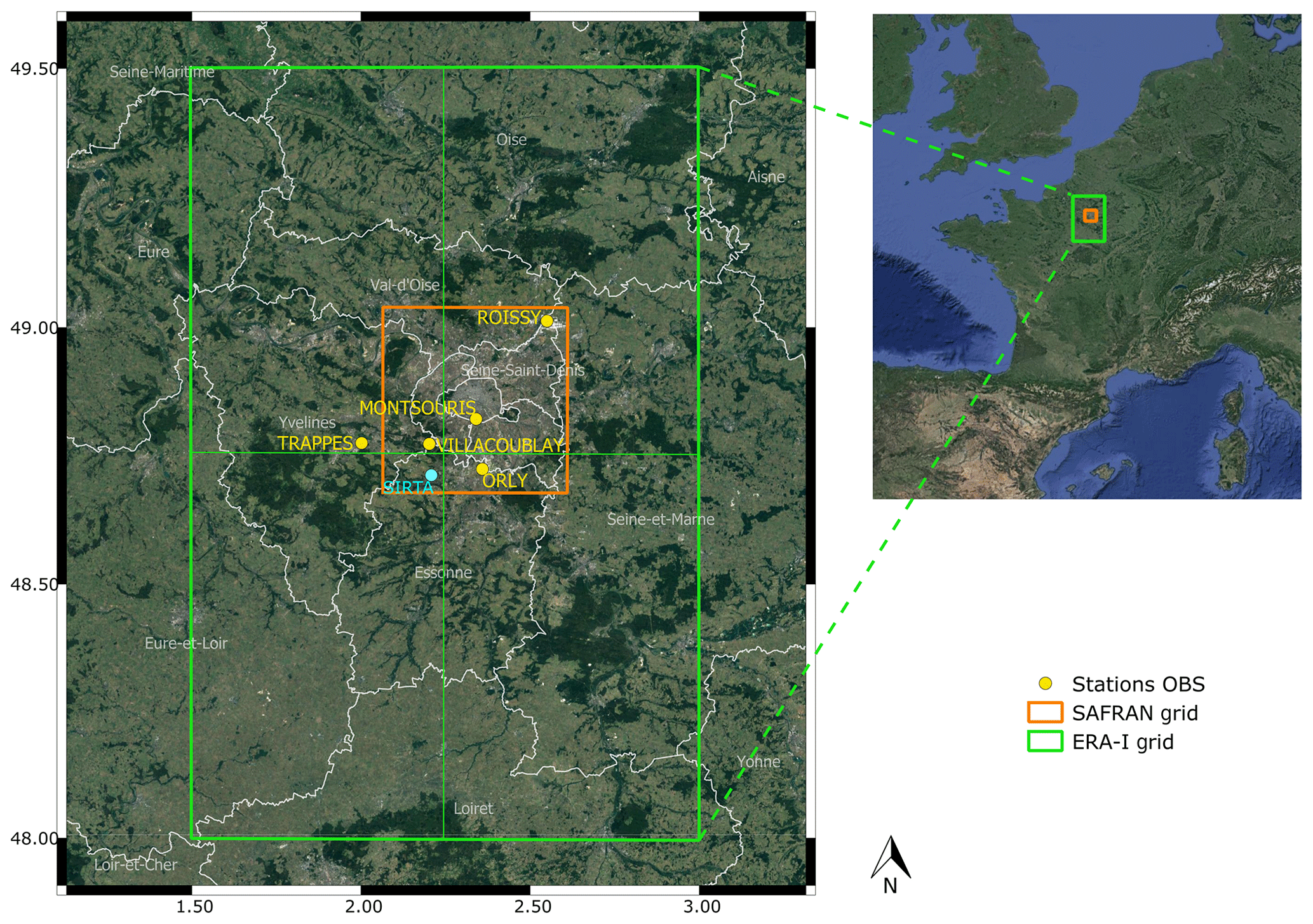
Figure 1Study area in the Paris region (France). Yellow: the Météo-France observation stations (OBS). Cyan: the SIRTA supersite. The green area represents the ERA-I coverage (4 pixels) and the orange area reflects the SAFRAN (Système d'Analyse Fournissant des Renseignements Adaptés à la Nivologie) coverage (36 detailed pixels; not shown).
The current paper examines changes in temperature distributions (T2 m, Tmax and Tmin), humidity (relative and specific) and precipitation at the following different timescales: annually, seasonally (winter – DJF; spring – MAM; summer – JJA; and autumn – SON) and especially during the summer season, according to the large-scale circulations; the paper also compares these changes between a past period (1979–2002) and current period (2003–2017). The observations used and their comparisons to reanalysis products are presented in Sect. 2 in order to check the ability of the commonly used atmospheric reanalyses to detect local-scale trends. Section 3 describes the methodology used to calculate trends and describe PDFs, as well as the method used to define continuous time weather regimes. In Sect. 4, trends and changes in distributions of the different parameters are analysed on an annual and seasonal scale. In Sect. 5, a focus is made on the summer season to analyse trends and distributions for the four main large-scale circulations. Section 6 discusses the results and their possible relationships according to the nature of the change (dynamic, thermodynamic or anthropic).
2.1 Observations
This study analyses climate trends at the local scale, in the region of Paris, France, from 1979 to 2017 using five Météo-France (MF) daily observation stations (in yellow in Fig. 1). The choice of these stations is motivated by (i) their good temporal sampling (few measurement gaps), (ii) their temporal availability, starting from at least 1979, and (iii) the fact that all considered variables are measured at the station. We performed a sensitivity analysis to compare the variability between each station as well as their differences with the ensemble of the five stations' mean. For all variables, the five stations show a very strong correlation between them (not shown). The Montsouris (Trappes) station, located downtown (outside) Paris, has slightly warmer (colder) temperatures but similar variability to the other stations. Regarding the relative humidity, Montsouris has slightly drier conditions and Trappes slightly wetter conditions. Note that the other three stations show a correlation and variability almost identical to the average of the stations. This is why the five stations are averaged together to obtain a single daily observation series corresponding to the “Paris region”. For the sake of comparison (Sect. 2.2 and Appendix A), for precipitation, the average of the four stations located within the SAFRAN (Système d'Analyse Fournissant des Renseignements Adaptés à la Nivologie) grid (in orange in Fig. 1) is computed.
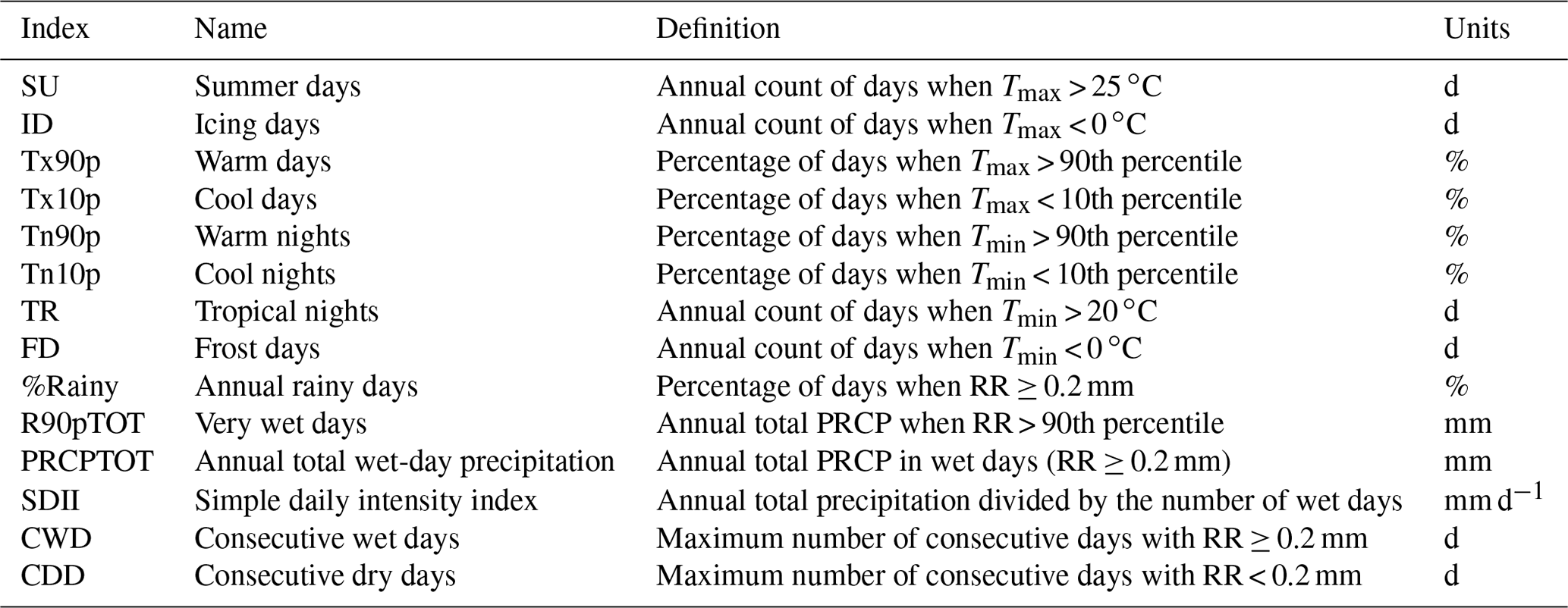
Based on these observations, we used the climate indices recommended by the joint CCl (WMO Commission for Climatology)/CLIVAR (World Climate Research Programme Project for Climate Variability and Predictability)/JCOMM (Joint Technical Commission for Oceanography and Marine Meteorology) Expert Team on Climate Change Detection and Indices (ETCCDI) (Karl et al., 1999; Peterson et al., 2001; Zhang et al., 2011) calculated from Tmax, Tmin and precipitation (PRCP) (Table 1). With regard to precipitation, the indices are generally calculated according to a threshold of 1 mm; this threshold differentiates a rainy day from a non-rainy day. In this study, we modified this threshold to 0.2 mm. This choice is motivated by the World Meteorological Organization (WMO), which recommends an accuracy of 0.2 mm for rain gauges (WMO, 2014), considering that minimal rainfall for a rainy day is 0.2 mm d−1. Finally, when the indices use percentiles, they are calculated on the annual series when looking at annual trends and calculated over the season when looking at seasonal trends.
Table 1Climate indices (temperature in the eight first lines and precipitation in the last six lines) based on Climdex indices. In this study, the threshold between a dry day and a rainy day (RR) is set at 0.2 mm d−1, unlike ETCCDI, which uses a threshold of 1 mm d−1.
2.2 Comparison of the local observation with the ERA-Interim reanalyses and SAFRAN analysis
Although the main data sources in this study come from direct observation, it is interesting to test the ability of well-known reanalyses to represent the fine-scale behaviour. To do so, we used the European Centre for Medium-Range Weather Forecasts (ECMWF) ERA-Interim reanalysis (Simmons et al., 2014), as well as the high-resolution meteorological analysis SAFRAN (Quintana-Seguí et al., 2008), for precipitation. ERA-I shows a general pattern of underestimation of temperatures (T2 m, Tmax and Tmin) relative to observations, which is more marked seasonally, especially in spring and summer (Fig. A1b and e in the Appendix). In addition, ERA-I also shows a strong overestimation of relative humidity annually and seasonally, whereas the specific humidity is rather well estimated by ERA-I. For precipitation, SAFRAN shows rather satisfactory results in terms of bias despite the high daily variability (Fig. A1b and e). However, the statistical analyses carried out on the monthly accumulations show very good results, confirming that SAFRAN is well adapted to inform the precipitation at local scale, at least for this area. The detailed results obtained from the two datasets are presented in Appendix A. The reasons for the discrepancies between direct observation and ERA-I/SAFRAN are out of the scope of this paper, but the presence of significant bias at this local scale motivates the use of observations and not reanalysis for the current issues.
2.3 Local climate
The temporal evolution of the six daily variables, namely, the daily temperature at 2 m (T2 m), the daily maximum temperature at 2 m (Tmax), the daily minimum temperature at 2 m (Tmin), the relative humidity (RH), the specific humidity (q) and PRCP, on an annual basis and for seasonal scales, is presented in Fig. 2. The local climate is characterized by cold and humid winters in contrast to warm and increasingly drier summers. The seasonal averages of T2 m and Tmax are similar in spring and autumn; however, autumn has warmer Tmin and wetter conditions than does spring. The relative humidity is the only variable for which the decrease tendency, especially in the spring–summer, clearly appears. Regarding precipitation, the Paris region shows no preferential season when considering the total amount.
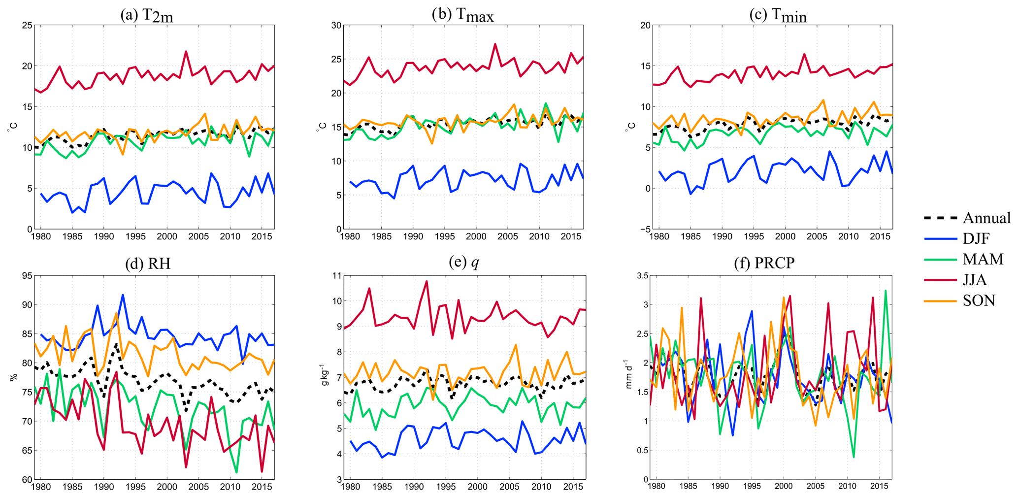
Figure 2(a) Annual averages (dashed black line) and seasonal averages (coloured lines) of T2 m (∘C), (b) Tmax (∘C), (c) Tmin (∘C), (d) RH (%), (e) q (g kg−1) and (f) daily PRCP average (mm d−1). DJF is in blue, MAM in green, JJA in red and SON in orange.
3.1 Mann–Kendall trend test
Trends were calculated using the Mann–Kendall test (Kendall, 1955; Mann, 1945). This test detects the presence of a monotonic tendency in a chronological series of a variable. It is a non-parametric method; that is, it makes no assumptions about the underlying distribution of the data, and its rank-based measure is not influenced by extreme values. This method mainly gives three types of information. The first piece of information is the Kendall tau, or Kendall rank correlation coefficient, which measures the monotony of the slope. Kendall's tau varies between −1 and 1; it is positive when the trend increases, and vice versa. The second piece of information is the Sen slope, which estimates the overall slope of the time series. This slope corresponds to the median of all the slopes calculated between each pair of points in the series. The third piece of information is the significance, which represents the threshold for which the hypothesis that there is no trend is accepted. The trend is statistically significant when the p value is less than 0.05.
3.2 Anomaly and normalization
To compare two periods, we use the probability density function of normalized anomalies. The data of an X variable are exploited as anomalies X′ with respect to climatology . Here, we take as climatology the whole period of study, the normal one of a day d of the year y, with d, ranging from 1 to 365, as the average of this day over the period 1979–2017 (Eq. 1) as follows:
with N number of years. To obtain a non-noisy signal, the climatology is smoothed by a locally weighted scatterplot smoother (LOWESS). Once the climatology is obtained, we calculate the daily anomaly (Eq. 2) as follows:
Monthly or seasonal anomalies are directly obtained by averaging over months or seasons. Finally, the anomalies X′(d) are normalized over the period 1979–2017 according to the temporal scale studied (t), where tϵ1, Nt (year or season) as follows:
with
We normalized the anomalies with respect to the entire 1979–2017 studied period because, according to Huntingford et al. (2013) and Sippel et al. (2015), when anomaly normalization is performed relative to a reference period, then standardization tends to increase the variability and extremes.
With a normalized anomaly, we compute the distributions for two periods (1979–2002 and 2003–2017). The choice of separation between these two periods is mainly motivated by the fact that over the 2003–2017 period observations of various meteorological parameters are available at the SIRTA supersite (see Fig. 1) and have been reanalysed to produce the SIRTA-ReOBS dataset at an hourly timescale (Chiriaco et al., 2018). This dataset is not used in this study, but it will be used in a forthcoming paper focused on the understanding of the processes responsible for the changes detected in the current paper.
3.3 Weather regimes
In winter and summer, climate variability in western Europe is controlled by different dynamic states called weather regimes (Cassou et al., 2005, 2011). These regimes are interpreted as quasi-stationary states of daily atmospheric circulation that can persist from a few days to a few weeks. Michelangeli et al. (1995) show that four regimes are relevant for the study of climate variability in the North Atlantic–European basin. These regimes are defined according to the geopotential height at 500 hPa or the sea level pressure (SLP) by the k-means method. Thus, each day is associated with a preferential regime (Legras and Ghil, 1985; Vautard, 1990; Yiou et al., 2008). Weather regime analysis allows observing climate trends at constant air mass; that is, large-scale circulation is fixed, and thus the variability detected is rather explained by smaller-scale processes. This study uses a regime classification, calculated from the SLP over a reference period of 1970–2010 and available at the following link (https://a2c2.lsce.ipsl.fr/index.php/deliverables, last access: 15 January 2019; for more details, see Cattiaux, 2010; Yiou et al., 2011, 2018). Such classification is efficient for stable seasons such as winter and summer, and less for spring and fall, which are transition seasons and therefore more subject to rapid large-scale changes. We mainly focused on summer because of the strong local variability related to the thermodynamical processes that affect the summer season and whose changes are more marked in summer than in winter.
In summer, there are four preferential regimes (Fig. B1 in Appendix B represents the anomalies of SLP associated with these four summer regimes). The North Atlantic Oscillation in its negative phase (NAO-) (Fig. B1) is characterized by a weakening of the Icelandic Low. The jet stream is pushed back to the south on its arrival in western Europe, causing cold conditions over most of Europe. In the Paris area, this regime is marked by cooler and wetter conditions. The Atlantic Ridge phase is characterized by high pressures over the Atlantic Ocean and low pressures over the northwest of Europe, favouring cold conditions via the reinforcement of a polar flux. On the other hand, it inflates the Azores anticyclone in its subtropical part and thus warms the rest of Europe. In the Paris area, this regime is marked by cool temperature and slightly humid conditions. The blocking phase is characterized by a strong anticyclone over the British Isles, which blocks the inflow of maritime air and allows warm conditions to develop in western Europe. Southeast Europe is rather cold. In the Paris region, this regime favours hot and dry temperature conditions. And finally, the Atlantic Low phase slows down the polar flow in favour of a southerly flow favourable to warm conditions over all of western Europe. In the Paris region, this regime favours warmer and drier conditions than other regimes.
Thus, each summer day of our study is associated with one of the four weather regimes above, and we can separate at first order the evolutions of the parameters due to circulation changes to those due to local changes.
In this section, the observed trends for several variables and climate extremes indices at the annual scale since 1979 are presented. Then, in a second step, each variable and each climate extreme index is studied at the seasonal scale.
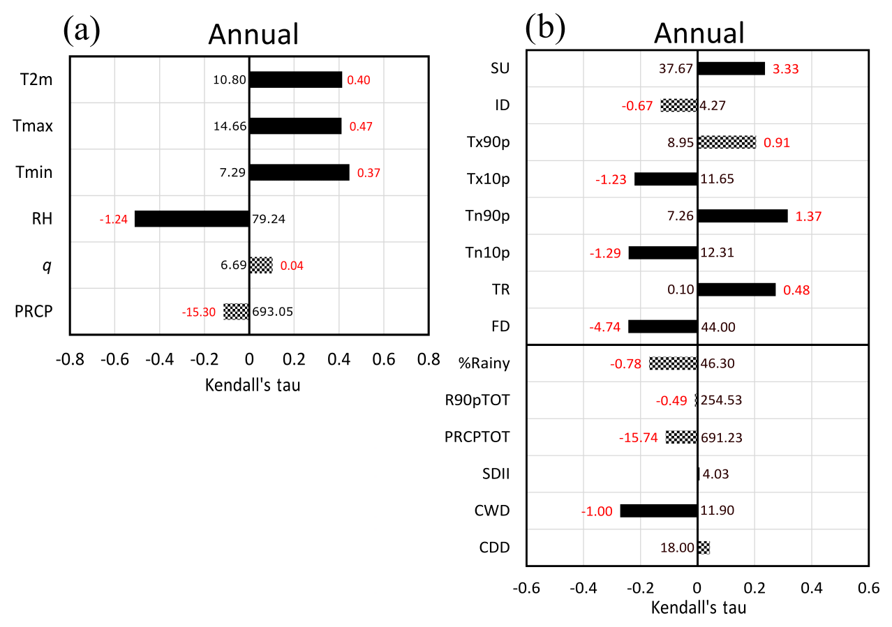
Figure 3Mann–Kendall annual trends in observational data for (a) T2 m, Tmax, Tmin, RH, q and PRCP, and for (b) climate indices from Tmax, Tmin and precipitation. On the abscissa, Kendall's tau represents the rank correlation coefficient between the variable and time. The red value represents the Sen slope, i.e. the median slope in units per decade, and the black value represents the average original value in 1979 (in units). A solid bar indicates a significant trend for a confidence interval of p=0.05, and a mosaic bar indicates a non-significant trend.
4.1 Annual trends
At the annual scale, Mann–Kendall trends from observations (Fig. 3a) show a significant increase in T2 m of approximately 1.6 ∘C since 1979 (0.4 ∘C decade−1), 1.9 ∘C for Tmax (0.47 ∘C decade−1) and 1.5 ∘C for Tmin (0.37 ∘C decade−1). In addition, as the Tmin Kendall tau is higher than that of Tmax, this means that although Tmin warms up less quickly than the Tmax, its increase is more monotonic. The relative humidity decreases significantly (4.3 %, i.e. 1.24 % decade−1) from 79.2 % (origin of Sen slope in 1979) to 74.5 % in 2017, and it appears to be guided by the temperature trend, as no significant trend is detected for specific humidity. For precipitation, despite an observed decline, there is no significant trend.
Figure 3b shows the trends, on an annual scale, of climate indices calculated from Tmax, Tmin and PRCP (see Table 1 for definition). For the warm part of the distribution, warm Tmin (Tn90p) increases significantly, and the number of summer days (SU) shifts from approximately 37.7 d in 1979 to 50.3 d in 2017. For the cold part of the distribution, Tx10p and Tn10p decrease significantly, as well as the number of frost days (FD) from approximately 44 d in 1979 to 26 d in 2017. For precipitation, only the maximum number of consecutive wet days decreases significantly, with a maximum period of consecutive rainy days equal to 12 d on average in 1979 and 8 d in 2017.
Hence, on an annual scale, in the Paris region, the changes of the last four decades are mainly on the relative humidity, which presents a strong decrease, and on the temperatures (average, maximum and minimum), with a shift of the distribution towards warmer temperatures leading to more warm days, fewer cold days and higher minimum and maximum temperatures, which is a rather typical trend, although Tmax presents a stronger positive trend than Tmin. No significant trend can be detected for precipitation because the variability is too great, except for the decrease of the maximum number of consecutive rainy days. This result is opposite to the one reported by Zolina et al. (2010), who found that wet spells increase over 60 years in Europe by approximately 15 % to 20 %. However, the period of study differs substantially as they carry out their analysis over the 1950–2008 period, and their threshold between a rainy and non-rainy day is 1 mm versus 0.2 mm for the current study. The analysis of precipitation can be sensitive to these differences and to local effects. It is expected that the decrease in relative humidity observed in the Paris area affects some indices of precipitation, especially indices concerning occurrence (Bastin et al., 2019).
4.2 Seasonal trends
4.2.1 Temperatures
For all seasons except winter, T2 m increases significantly (Fig. 4a), approximately 2.1 ∘C (0.52 ∘C decade−1) in spring and 1.8 ∘C (0.46 ∘C decade−1) in summer, with a strong positive monotonic relationship (Kendall's tau). Warming is also significant for Tmax (Fig. 4b) and Tmin (Fig. 4c) at all seasons except for DJF. Tmax increases strongly in MAM (2.9 ∘C, i.e. 0.73 ∘C decade−1) and JJA (2.1 ∘C, i.e. 0.52 ∘C decade−1), while the Tmin increase is slightly weaker (1.6 ∘C, i.e. 0.41 ∘C decade−1 in MAM, 1.8 ∘C, i.e. 0.46 ∘C decade−1 in JJA). However, the Kendall tau of Tmin is greater than 0.4 in JJA; this is the largest tau for all temperatures and all seasons, reflecting a constant increase in Tmin in JJA since 1979.
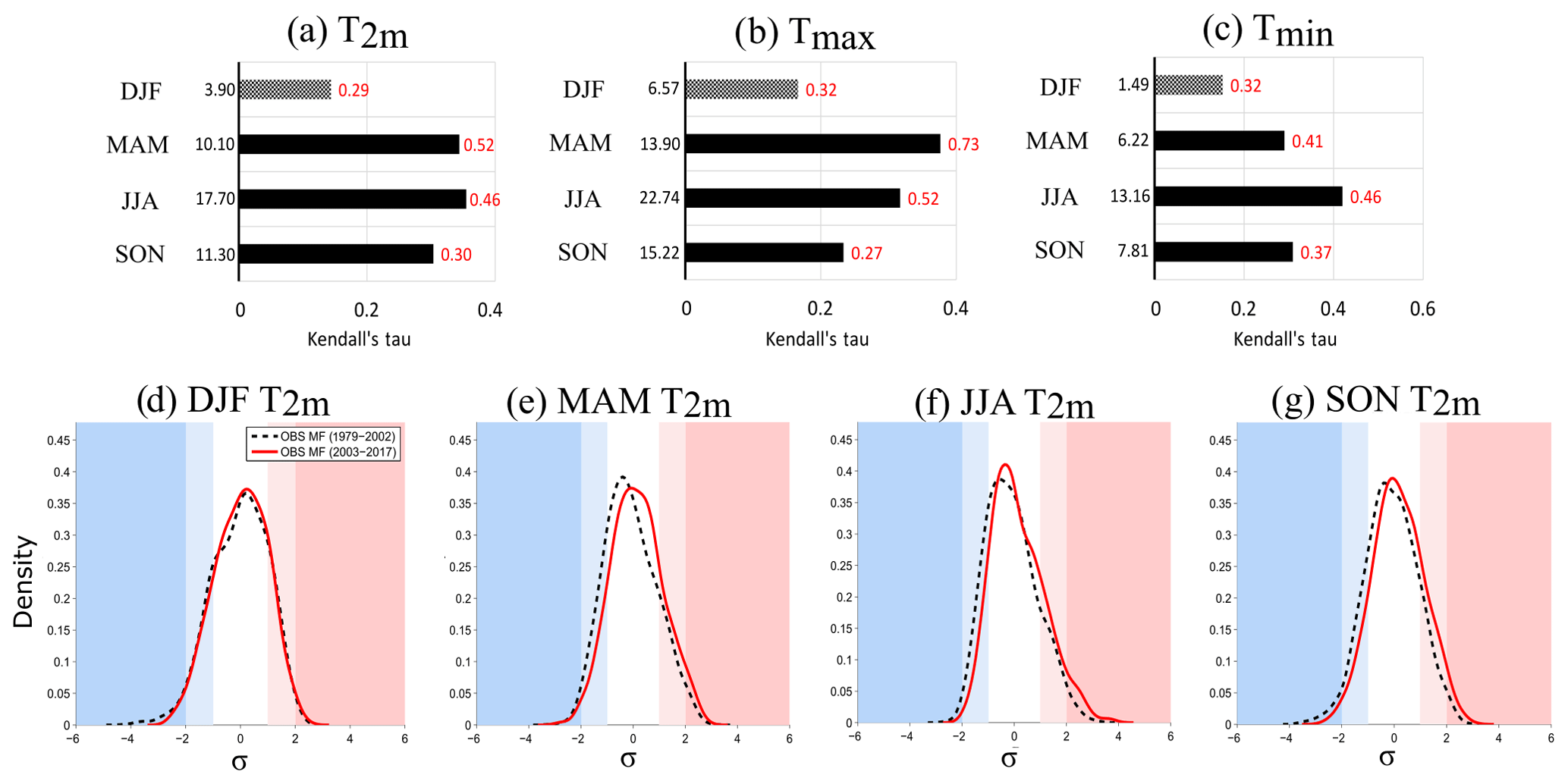
Figure 4Top: Mann–Kendall seasonal trends in observational data for (a) T2 m, (b) Tmax and (c) Tmin. Characteristics of the figure are the same as for Fig. 3. Bottom: seasonal PDF of the daily anomalies of T2 m, normalized over the period 1979–2017, for (d) DJF, (e) MAM, (f) JJA and (g) SON. Dashed black line: the past period from 1979 to 2002; red line: the current period from 2003 to 2017. The white part of the figure corresponds to [−1 < σ < + 1], light colours to [−2 < σ < −1; 1 < σ < 2] and dark colours to [σ < −2; σ > 2].
In terms of PDF and extremes, DJF shows little change in the mean of the PDF (Fig. 4d), but the number of very cold anomalies of T2 m (<−3σ) decreases. The same results are observed for Tmax and Tmin (not shown), but there are no trends in temperature climate indices (Fig. 5a).
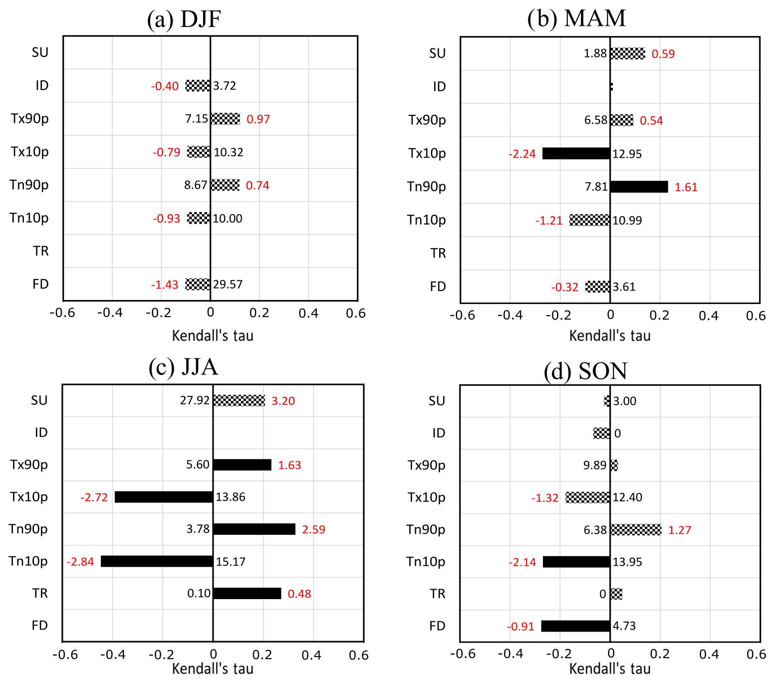
Figure 5Mann–Kendall seasonal trends of temperature climate indices calculated from Météo-France observations stations for the four seasons: (a) DJF, (b) MAM, (c) JJA and (d) SON. See Table 1 for temperature climate indices. On the abscissa, Kendall's tau represents the rank correlation coefficient between the variable and time. The red value represents the Sen slope, i.e. the median slope in units per decade, and the black value represents the average original value in 1979 (in units). A solid bar indicates a significant trend for a confidence interval of p=0.05, and a mosaic bar indicates a non-significant trend.
In MAM (Fig. 4e), the average of the T2 m anomalies over the current period increases, marked by a shift of the PDF to the right, which means more warm anomalies. The number of days where Tmax is lower than the 10th percentile (Tx10p) decreases (Fig. 5b), consistent with the strong increase in Tmax for this season. On average, Tmax warms up very strongly (2.9 ∘C in 39 years, from approximately 13.9 to 16.7 ∘C; Fig. 4b), with constant behaviour (strong Kendall tau; Fig. 4b). However, there is no change in the cold anomalies' tail of the distribution of Tmax (not shown). This indicates that the presence of very cold events persists in spring but with a decline in frequency (Tx10p; Fig. 5b). Figure 5b also shows that the percentage of days when the minimum temperature is greater than the 90th percentile (Tn90p) increases in spring.
In JJA (Fig. 4f), the average T2 m anomalies increase (PDF less flattened and shifted to the right), as well as very warm anomalies greater than 2σ. The same characteristics of PDF evolution are observed on Tmax and Tmin (not shown). The temperature indices show strong significant trends (Fig. 5c). The cold indices (Tx10p and Tn10p) decrease continuously, whereas warm indices (Tx90p, Tn90p, TR) increase. In summer, high values of Tmin (higher than the 90th percentile) were reached for 3.8 % of the days in the past compared with 13.6 % now; at the same time, the lowest temperatures (10th percentile) were reached for 15.7 % of the summer days in the past and only 4.4 % of present days. These trends are linked to the strong increase in Tmax and Tmin observed in JJA and in particular the right shift of the PDF.
In SON (Fig. 4g), the same as for the other seasons, the average T2 m anomalies increase, cold anomalies are less cold and warm anomalies are more likely to occur. Tmax and Tmin show the same characteristics. Significant trends are observed for the coldest temperature indices (Fig. 5d). The number of days where the Tmin is less than the 10th percentile (Tn10p) and the number of days where the Tmin is below 0 ∘C (FD) decrease significantly. These results come from the increase in Tmin (1.5 ∘C), which in autumn is larger than for the Tmax (1.1 ∘C).
In summary, the largest temperature changes appear in MAM and JJA. Spring shows a strong increase in temperatures, but climate indices show fewer changes due to variability, allowing the presence of punctually cold Tmax and Tmin. In summer, the temperatures increase strongly, as do the very warm anomalies higher than 2σ; warm (cold) extremes are more (less) frequent. In the autumn, cold extremes decrease due to the stronger increase of Tmin than Tmax.
4.2.2 Humidity
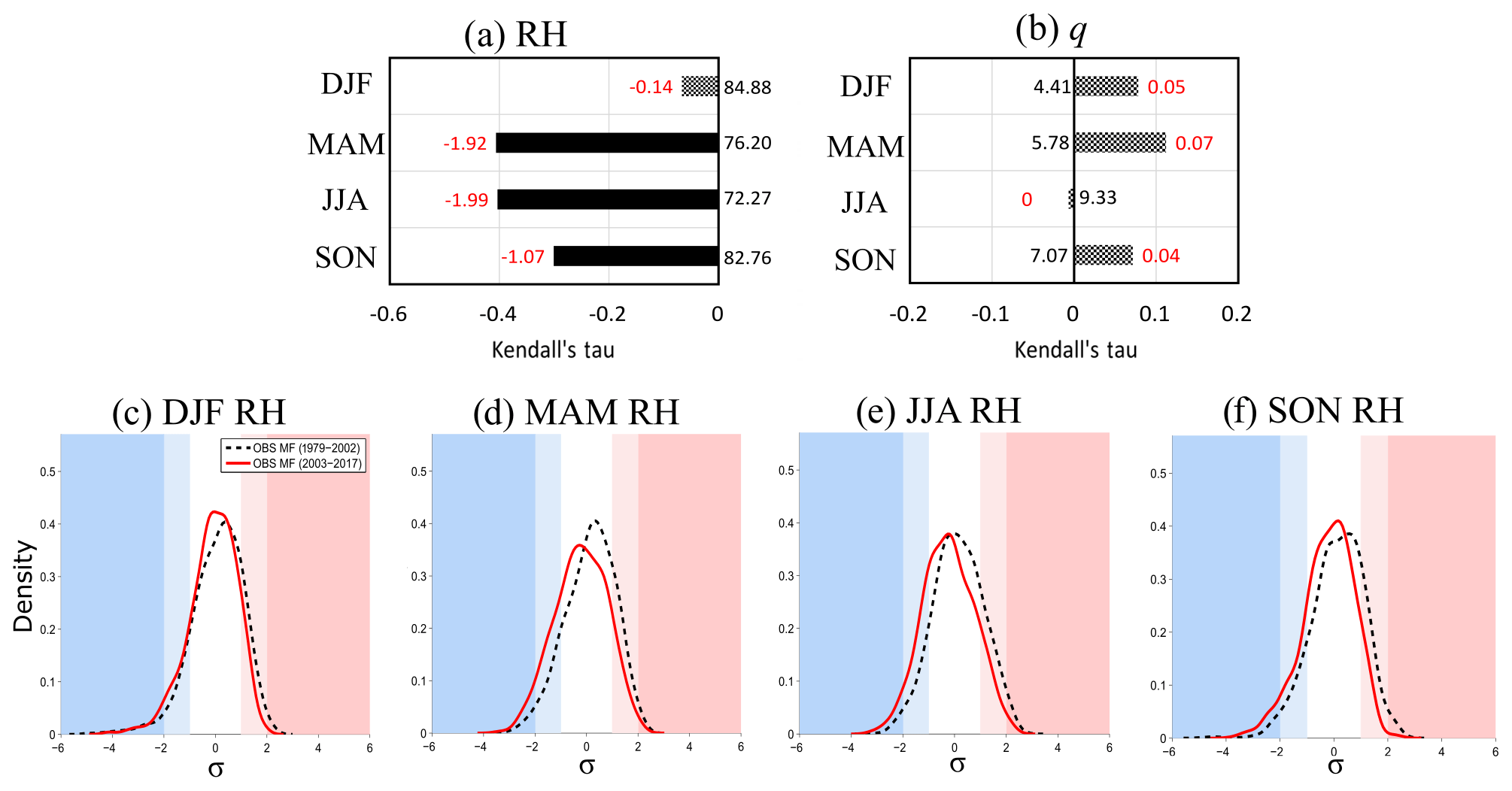
The relative humidity (Fig. 6a) decreases significantly in all seasons except DJF. This is due to the fact the specific humidity increases are less than what could be expected by Clausius–Clapeyron, according to the increase of the temperature. Indeed, specific humidity shows no significant trends and even shows a slope of zero in JJA (Fig. 6b). The strong monotonic decrease of RH is approximately 7.7 % (1.92 % decade−1) in MAM and 8 % (1.99 % decade−1) in JJA. For JJA, RH shows an average value of 72.3 % in 1979 and decreases to 64.7 % on average in 2017. This strong decrease in relative humidity is observed on PDFs (Fig. 6c–f). For all seasons, the average of the anomalies decreases (current PDF shifted to the left). However, this shift is more marked in MAM (Fig. 6d) and JJA (Fig. 6e). In addition, DJF shows little change in the extremes (Fig. 6c), while in MAM and JJA, the number of moist anomalies decreases, and the number of dry anomalies increases. Finally, in SON, the number of very humid anomalies decreases, and the number of very dry anomalies increases (Fig. 6f).
In summary, in spring, summer and autumn, the evolution of RH distribution leads to a decrease in the frequency of humid anomalies (very humid anomalies in autumn) and an increase in the frequency of dry anomalies (very dry anomalies in autumn). This decrease appears to be guided by the temperature trend, as the amount of water in the atmosphere near the surface, i.e. specific humidity, remains almost unchanged in all seasons.
4.2.3 Precipitation
At the seasonal scale, the trends in rainfall are not significant (Fig. 7a). Figure 7b–e shows the PDFs of observed daily intensities only for rainy days (> 0.2 mm d−1) for the past period (1979–2002) and the current period (2003–2017). In DJF (Fig. 7b), the frequency of daily intensity decreases over the current period, also observed on climatic indices with a decrease in R90pTOT (Fig. 8a). In addition, the maximum number of consecutive wet days (CWD) decreases (Fig. 8a) from approximately 10.1 to 6.8 d. In MAM, the extreme intensities of precipitation are slightly more frequent over the current period (Fig. 7c). Furthermore, Fig. 8b shows a decrease in the percentage of rainy days (% rainy), a decrease in the maximum number of consecutive wet days (CWD) and an increase in the maximum number of consecutive dry days (CDD). The spring shows, on average, 48.5 % of rainy days in 1979 versus 36.3 % in 2017, and the average maximum periods of consecutive dry days evolve from 8.7 to 15.4 d. In spring, the weather is drier, with fewer rainy days but slightly more extremes. This is consistent with the decrease in relative humidity that affects the triggering of precipitation (Bastin et al., 2019; Rasmussen et al., 2017). In JJA (Fig. 7d), the frequency of mean intensities (PRCP between 12 and 20 mm d−1) increases and the frequency of extreme intensities decreases. However, in JJA, despite all rainfall indices showing an increase, none is significant (Fig. 8c). In SON (Fig. 7e), the frequency of daily intensity decreases over the current period, a result also observed with the significant decrease of the SDII (Fig. 8d), i.e. a decrease in the daily mean intensity.
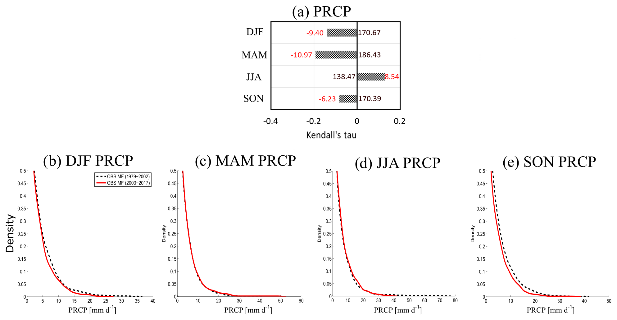
Figure 7(a) Same as Fig. 4a but for PRCP. Bottom: seasonal PDF of daily intensities of rainy days only (> 0.2 mm d−1) for (b) DJF, (c) MAM, (d) JJA and (e) SON. Dashed black line: the past period from 1979 to 2002; red line: the current period from 2003 to 2017.
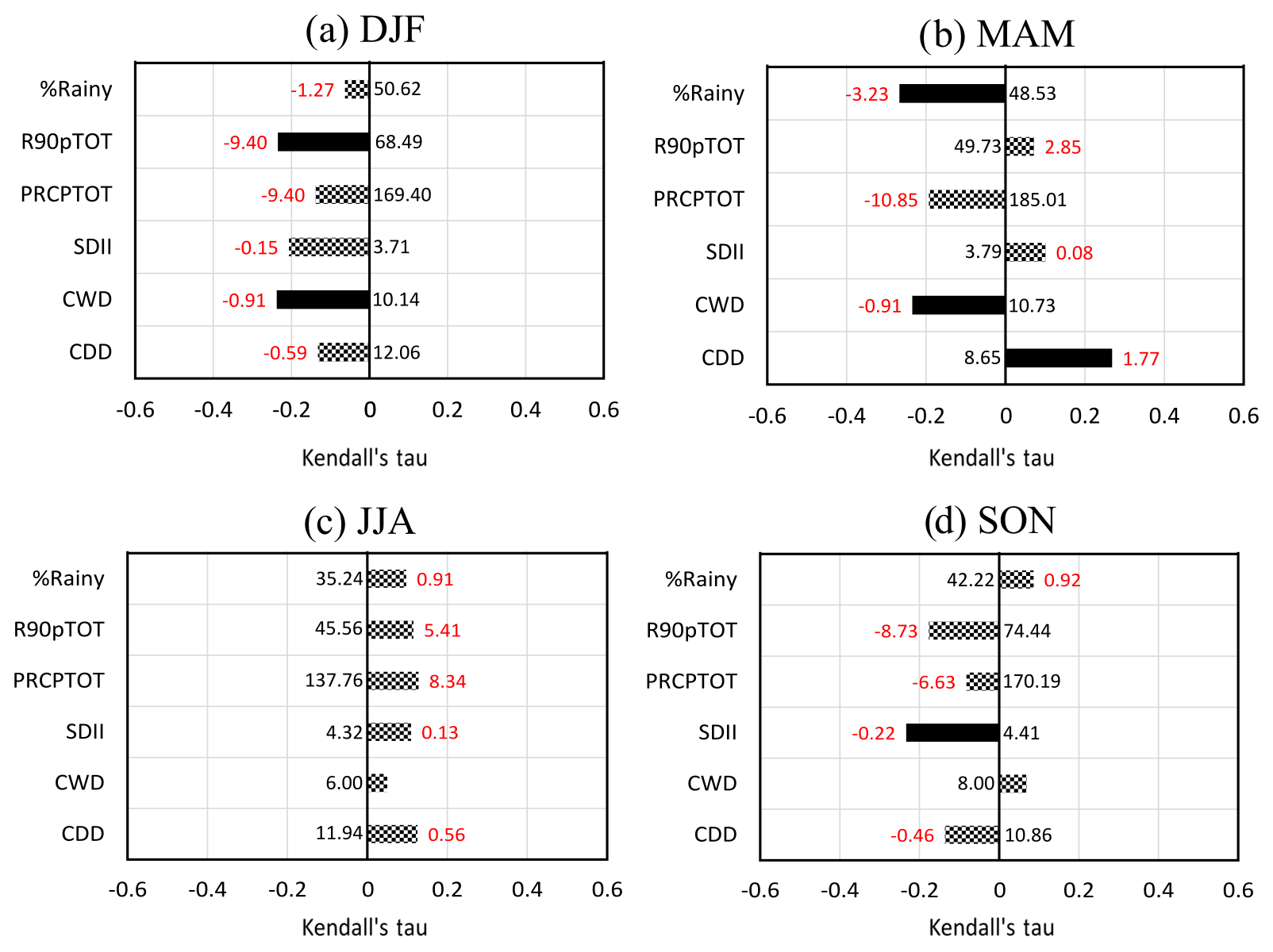
In summary, the high variability of precipitation does not allow the detection of significant trends for most climate indices. Nevertheless, the indices emphasize some results: extremes of precipitation occur less frequently in DJF, MAM becomes drier but heavy precipitation is stronger, JJA shows no significant trends and SON is marked by a decrease of the mean daily intensity.
The analysis shows that unexpected changes are occurring in summer at first order: precipitation exhibits an increasing trend (not significant), while it is the only season for which the specific humidity does not increase. To further study this season, it is necessary to understand what happens for each of the main atmospheric circulations. In the following section of this study, we focus on the summer season and we perform our trend analyses independent of large-scale circulations in order to characterize the changes coming only from thermodynamical processes.
Changes in temperature, relative humidity and precipitation, both in trends and distribution patterns, are more pronounced in spring and summer. The intraseasonal changes are identified based on a classification of each summer day based on weather regimes, which allows characterizing both the changes associated with large-scale circulation (in frequency) and the changes within each weather regime. Van Oldenborgh et al. (2009) and Vautard and Yiou (2009) found that changes in atmospheric circulation are not the main drivers of surface weather patterns in summer, unlike in winter. Indeed, local physical processes play a major role in summer variability. In the rest of this study, we focus on summer rather than spring because (i) the large-scale dynamics are more stable, which allows the definition of weather regimes and then the separation of the variability due to the large scale from that due to more local processes, (ii) the relative humidity decreases significantly in summer and spring, but the increase (non-significant) of specific humidity is particularly reduced in summer, and (iii) the evolution of precipitation indices in MAM is consistent with the decrease of relative humidity but not those in summer. For each regime, the percentages of frequency are computed for the past period (1979–2002) and the current period (2003–2017). The frequency of NAO- and Atlantic Low regimes increased by 9.1 % and 3 %, respectively; and the frequency of Atlantic Ridge and blocking regimes decreased by 5.9 % and 6.2 %, respectively. Using the weather regimes, we can write the temperature T2 m (or precipitation PRCP) as the sum, for the four regimes, of the occurrence of regime i* the mean value of temperature (or the daily mean intensity of precipitation – RR) in this regime. Then, between the two periods, we can calculate the dynamical and thermodynamical contributions of the change of the variable considered (ΔT for temperature or ΔPRCP for precipitation) adapted from Cassano et al. (2007) and Screen (2017) according to the following equations:
with
For example, with precipitation for a weather regime i, Δfi and are, respectively, the difference in the frequency of occurrence of the regime between the two periods and the mean value of frequency of occurrence in the past period; ΔRRi and are, respectively, the difference in the daily mean intensity of the precipitation between the two periods and the daily mean intensity of the precipitation in the past period. Then, is considered the dynamical term (change of precipitation due to dynamical change), the thermodynamical term (change of precipitation due to thermodynamical change) and (Δfi⋅ΔRRi) is the residue.
The partitioning method used in the paper to determine the dynamical and thermodynamical contributions of the trend is widely used (Cassano et al., 2007; Horton et al., 2015; Screen, 2017; Uotila et al., 2007). This method assumes that each weather regime is stationary in time. Hence, the dynamical contribution corresponds to the changes in the occurrence frequency of each circulation pattern, assuming that the circulation patterns are the same during the two periods (but they have been computed over all years covering at least the two periods so that the differences between the two periods are minimized). The thermodynamical contribution inside a weather regime is the result of influences unrelated to circulation, such as changes in long-wave radiation from increasing greenhouse gas concentrations or different cloud macro- and microphysical macro and microphysics properties, or changes in surface fluxes of moisture and/or radiation. The third component represents the interaction between dynamic and thermodynamic changes, and captures contributions that result from changes in the dynamical component acting on changes in the thermodynamical component.
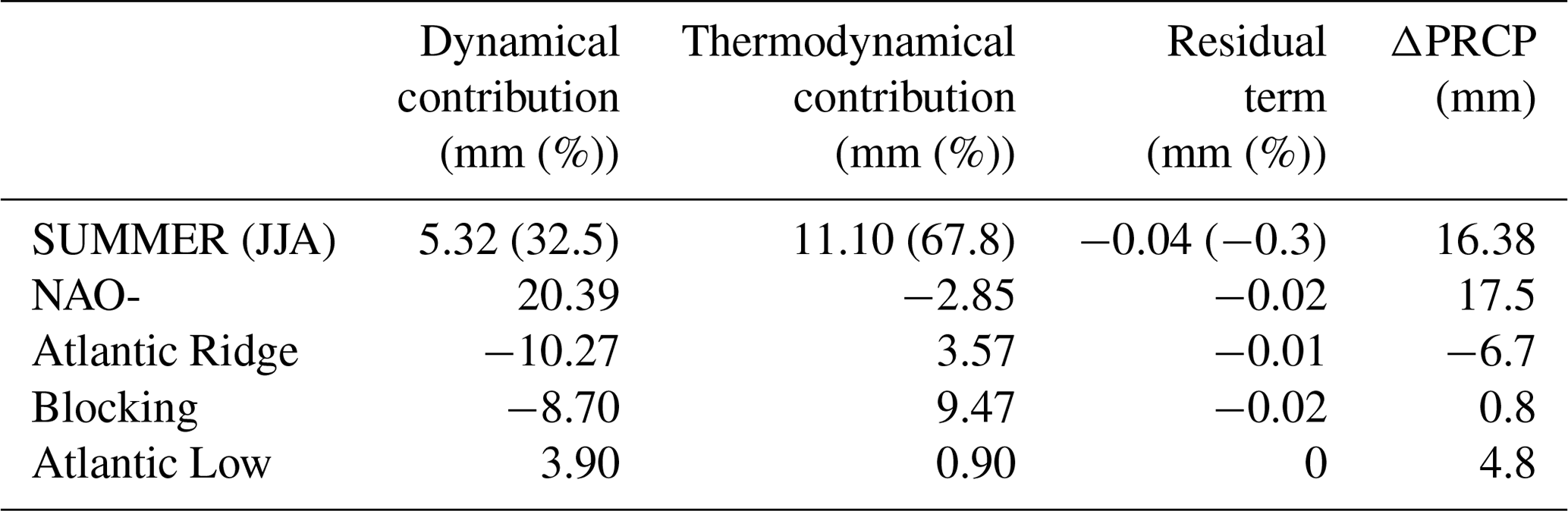
Using Eq. (7), in summer, the precipitation changes observed (Table 2) are explained at 67.8 % by the thermodynamical contribution and 32.5 % by the dynamics of occurrence, whereas at the weather regime timescale, the dynamics of occurrence are greater than the thermodynamics (i.e. contribution in millimetres).
Table 2Dynamical, thermodynamical and residual contributions of the precipitation change (ΔPRCP) in millimetres for summer (JJA) and for the four weather regimes in summer. Values in brackets give the ratio (in %) between the change components and the total change.
For climatic indices based on percentiles, we computed one value of the percentiles using the distribution of the entire summer season and the whole period but not a value for each weather regime. In this way, it is possible to characterize the evolution of each index inside a regime but also to compare the indices between regimes.
5.1 NAO-
The NAO- regime is characterized by a weakening of the Icelandic Low. Conditions are generally cooler over most of Europe. Since 1979, for NAO-, T2 m increases significantly by 1.9 ∘C (0.49 ∘C decade−1; Fig. 9), Tmax by 2 ∘C (0.52 ∘C decade−1; not shown) and Tmin by 1.8 ∘C (0.45 ∘C decade−1; not shown). This weather regime shows the largest increase in T2 m (and Tmin) compared to other summer regimes. Climatic indices' trends are not significant (Fig. 10a), but we observe fewer days below the 10th percentile for Tmin and Tmax and more hot days, while it is a weather regime associated with fresh conditions. Specific humidity (Fig. 9) shows little difference in the distribution, although most humidity is advected from the Atlantic Ocean during this regime. Such an evolution, associated with a temperature increase, is consistent with a decrease in the relative humidity (Fig. 9), but this decrease is weaker than for the other summer regimes. Rainfall increases but not significantly (Fig. 9 and PRCPTOT; Fig. 10a). NAO- is the only weather regime that shows an increase in PRCPTOT (Fig. 10); the intensity of this increase (∼8 mm decade−1) corresponds to the total increase observed in JJA (Fig. 8). Two reasons could explain this trend: precipitation increases during this regime (occurrence or intensity by event or both), or this trend is related to the increase in the number of days in NAO-. By applying Eq. (8) to determine the origin of change in precipitation between the two periods, the results presented in Table 2 show a contribution of the dynamical term, which is preponderant over the thermodynamical term, +20.39 and −2.85 mm, respectively, mainly explained by an increase in the frequency of occurrence of days in NAO- (+9.1 %, i.e. approximately 8 d). Furthermore, (1) the mean and median daily precipitation values are the same between the two periods (Fig. 9), and (2) the mean intensity of rainy days (SDII; Fig. 10a) and the percentage of rainy days (% rainy; Fig. 10a) show almost zero trends. All of these reasons confirm that the increase in PRCPTOT in NAO- (hence, in JJA) is more related to an increase in the occurrence of days in NAO-.
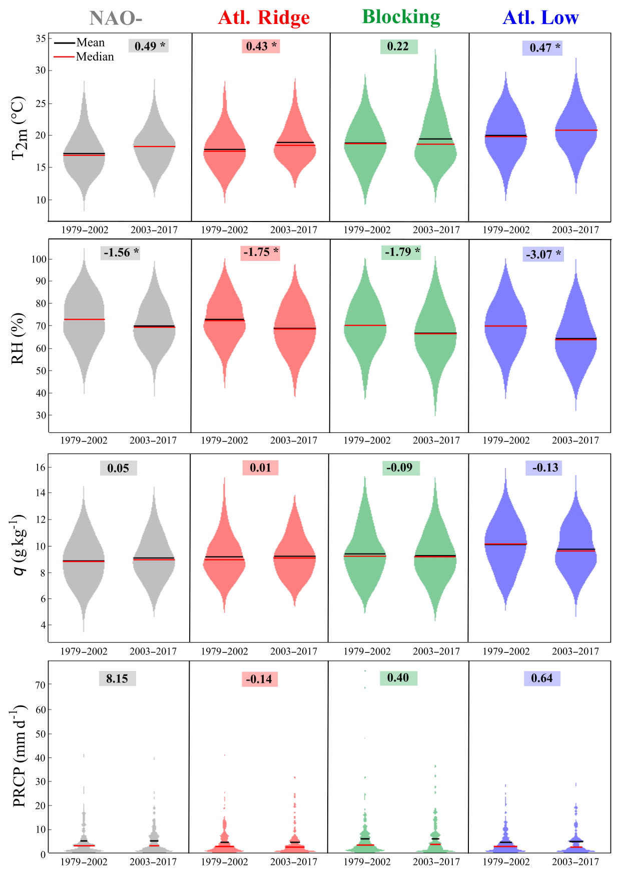
Figure 9Violin plot of daily T2 m (first line), RH (second line), q (third line) and PRCP (fourth line) for the four summer weather regimes between the periods 1979–2002 and 2003–2017 (one regime, one column). The black bar represents the mean, and the red bar represents the median. Boxed numbers represent trends in units per decade over the period 1979–2017. The asterisk represents a significant trend for a confidence interval of p=0.05.
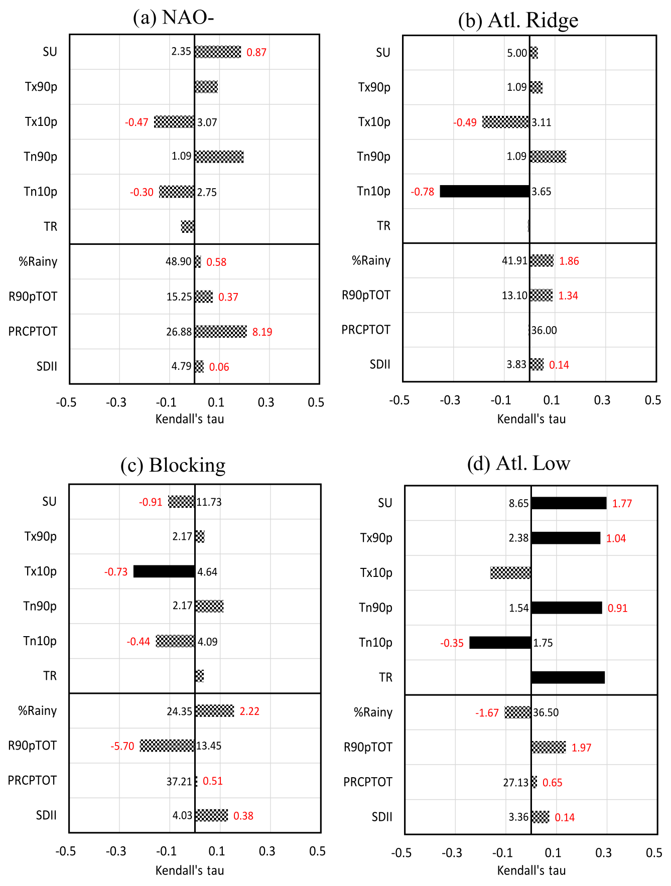
Figure 10Mann–Kendall trends in observational data for climate indices for the four summer weather regimes: (a) NAO-, (b) Atlantic Ridge, (c) blocking and (d) Atlantic Low. Figure characteristics are the same as for Fig. 7.
5.2 Atlantic Ridge
The Atlantic Ridge regime is characterized by high pressures over the Atlantic Ocean and low pressures over northwestern Europe, favouring cold conditions through the enhancement of polar flux towards western Europe. On the other hand, it inflates the Azores anticyclone in its subtropical part and thus warms the rest of Europe. Under this regime, the temperatures over the Paris area increase significantly for T2 m (1.7 ∘C, i.e. 0.43 ∘C decade−1; Fig. 9b) and especially for Tmin (1.8 ∘C, i.e. 0.45 ∘C decade−1; not shown). Warm and very warm anomalies are more frequent, but most striking is the change of shape of the violin, with a crushing of the bottom of the distribution and a stretching of its top. The number of days with a minimum temperature below the threshold of the 10th percentile (Tn10p; Fig. 10b) decreases in accordance with the consequent increase in Tmin. The relative humidity decreases (7 %, i.e. 1.75 % decade−1; Fig. 9), and this decline is completely driven by the temperature increase, as specific humidity shows no trend except a decrease in its variability during the current period (Fig. 9). Finally, there is no trend for precipitation (Fig. 9), which is linked to the fact that the thermodynamic tends to increase the precipitation (Table 2), while the atmospheric circulation tends to decrease the occurrence of this regime (Fig. 9).
5.3 Blocking
The blocking regime is defined by a strong anticyclone over the British Isles, which blocks the inflow of maritime air and allows warm conditions to develop, especially over western Europe. For this regime, the Paris area is isolated from the oceanic advection, and local processes become even more influent on the climate variability. On average under this regime, only Tmin warms up significantly (1.1 ∘C or 0.28 ∘C decade−1, not shown). The T2 m violin plots show the same median for the two periods (Fig. 9) but a warmer mean due to the upward distribution and more hot extremes for the current period. The stretching of this side of the distribution is also observed for Tmax and Tmin (not shown). The percentage of days with a maximum temperature below the 10th percentile (Tx10p; Fig. 10c) decreases from approximately 4.6 % in 1979 to 1.9 % in 2017. The relative humidity also decreases (7.2 %, i.e. 1.79 % decade−1; Fig. 9), marked by an increase in the occurrence of events with low relative humidity. Specific humidity does not change (Fig. 9). For precipitation, there is no significant trend (Fig. 9); however, there is an increase in the frequency of rainy days and a decrease in the contribution of very wet days (Fig. 10c), which is not a consistent result with Vautard and Yiou (2009) at the European scale. It is the only regime in which the thermodynamical contribution to the change of precipitation is greater than the dynamical contribution (Table 2). However, these two contributions compensate for each other, because the dynamical term explains the decrease in precipitation variation up to −8.7 mm (Table 2), whereas the thermodynamical term explains the increase in precipitation variation up to +9.47 mm. We observe a change of precipitation in blocking, which is not visible on the trends because this change is compensated by a decrease in the frequency of occurrence of the number of days in blocking (6.2 %, i.e. approximately 5.6 fewer days).
5.4 Atlantic Low
The Atlantic Low regime slows polar flow in favour of a southerly flow favourable to warm conditions throughout western Europe. This regime shows the greatest changes in terms of trends (Fig. 9) from the point of view of T2 m, Tmax and Tmin, and a strong significance of trends on temperature extremes (Fig. 10d). The T2 m increases by 1.9 ∘C (0.47 ∘C decade−1), the Tmax by 2.3 ∘C (0.58 ∘C decade−1) and the Tmin by 1.7 ∘C (0.42 ∘C decade−1). Warm and very warm anomalies increase, and cold anomalies decrease. The relative humidity decreases very strongly, by approximately 12.3 % (3.07 % decade−1; Fig. 9), from approximately 72 % to 60.3 % in 39 years, while there is no trend for specific humidity on average. However, the median and the mean of the current box plot are slightly lower, and the shape of the violin is strongly modified between the two periods, with the emergence of a bimodal distribution (Fig. 9). Precipitation and extreme rainfall indices show no trends (Figs. 9 and 10d), but once again some differences between the two distributions appear, with a bimodal shape and a small increase in the occurrence of the number of days in Atlantic Low (3 %, i.e. 2.7 d), accounting for only +3.9 mm of the precipitation change observed (Table 2).
5.5 The contribution of regimes to warm extremes
Blocking and Atlantic Low are the two regimes that favour hot conditions in summer. Most heat waves over Europe occur when the blocking or Atlantic Low regimes are installed (e.g. Cassou et al., 2005). We have seen previously that the largest trends are observed for the Atlantic Low and that blocking shows the weakest trends for temperature. If we focus on the SU (Table 1), i.e. the number of days with Tmax > 25 ∘C, the blocking (Fig. 11, green) and Atlantic Low (Fig. 11, blue) regimes are the two regimes showing the highest frequency of SU. Figure 12 shows the evolution of the SU (number of summer days per year) for the JJA season and for each regime. In this figure, we compute the trend for different segment sizes (minimum size of 5 years); the x axis indicates the first year and the y axis the final year. Red (blue) colour indicates an increasing (decreasing) trend. When considering the entire period (starting from 1979), SU increases, but this is not the case when reducing the period and starting from the middle end of the 1990s, reinforcing the idea of a temperature warming slowdown in the 2000s, although there is still no consensus on the existence of a hiatus at the global scale, with the slowdown being the result of internal climate variability (e.g. Dai et al., 2015). The increasing trend in SU over the season (Fig. 12a) is partly due to the increase of these events during the Atlantic Low weather type (Fig. 12e), as well as in the NAO- starting from the end of 1990 (Fig. 12b). The blocking regime, which is suitable for heat waves, shows a decrease of SU. This is associated with a decrease in the frequency of Tmax ranging from 25 and 30 ∘C, even if there are more events with an increase of Tmax above 30 ∘C (Fig. 13). There is therefore an increase in episodes of very intense heat in blocking, which is not detectable via the SU index (Fig. 12d). Similar analysis can be done for the warm Tmin (Tn90p; not shown), which is predominant in blocking and in the Atlantic Low, and which is an important factor in heat wave definition. In terms of trends, the occurrence of warm Tmin increases in summer over the entire period, which is linked to an increase of events during the Atlantic Low from 1980 to the 2000s, followed by an increase of events during NAO- starting from the 2000s.
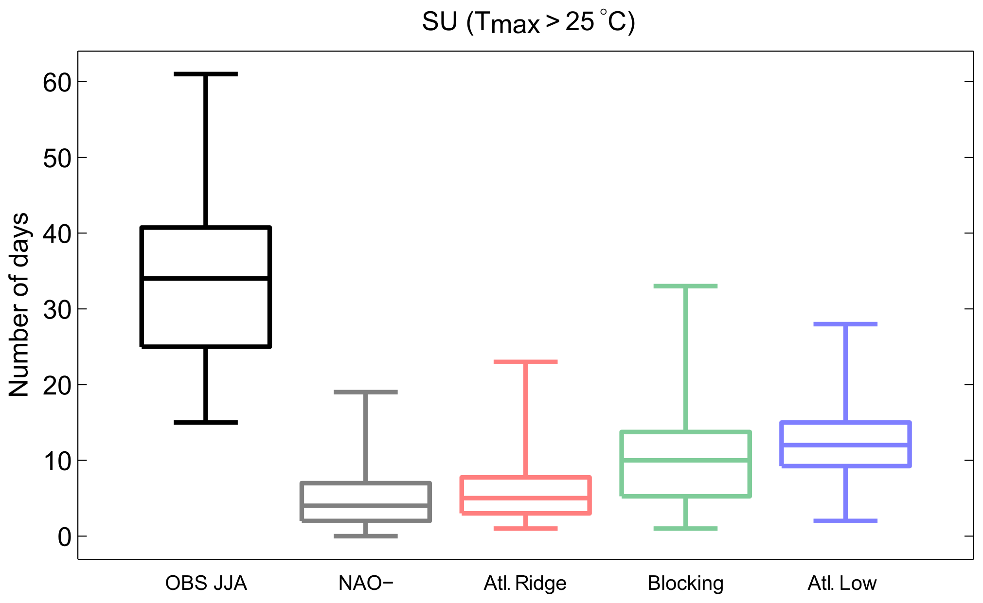
Figure 11SU frequency (Tmax > 25 ∘C) in number of days for the JJA season (black box plot) and for each summer weather regime calculated over the period 1979–2017. The bottom and top edges of the box indicate the 25th and 75th percentiles, respectively, and the central line is the median. The bottom and top lines outside the box indicate the minimal and maximal values, respectively.
In summary, the “hot” weather regimes (Atlantic Low and blocking) continue to contribute to extreme temperature events. However, the NAO- regime, with colder and wetter conditions compared to the first two regimes, shows strong warming trends, which leads to an increasing number of warm extremes starting from the 1990s, thus increasing the total probability of extreme events in summer in the Paris area.
On an annual scale, the climate of the Paris area has changed during the last four decades mainly due to warmer temperatures (average, maximum and minimum), with more warm extremes, fewer cold extremes and a strong decrease of the relative humidity. No significant changes are found for the specific humidity or precipitation. The rate of warming is similar to that observed in the rest of western Europe (Van Oldenborgh et al., 2009; Xoplaki, 2005). However, we observe a stronger increase in Tmax than in Tmin over the last 40 years, whereas Donat and Alexander (2012) observed the opposite across different regions of the globe starting from the middle of the 20th century. In addition, they concluded that daily temperatures have become “more extreme” and that these changes are related to changes in the mean but also in the extremes; this result is also observed in our trends. One issue is to determine if the changes we found can be attributed to dynamic, thermodynamic or local anthropogenic modifications.
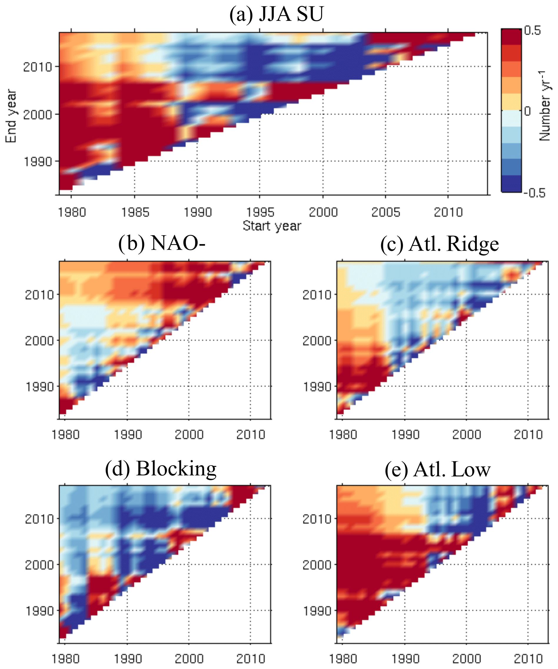
Figure 12Linear trends of SU (in number of d yr−1) as a function of length of segment (the y axis represents the end year of the segment, and the x axis represents the starting year of the segment) for (a) summer, (b) NAO-, (c) Atlantic Ridge, (d) blocking and (e) Atlantic Low. The minimum segment size is 5 years, and the trend is calculated by linear regression.
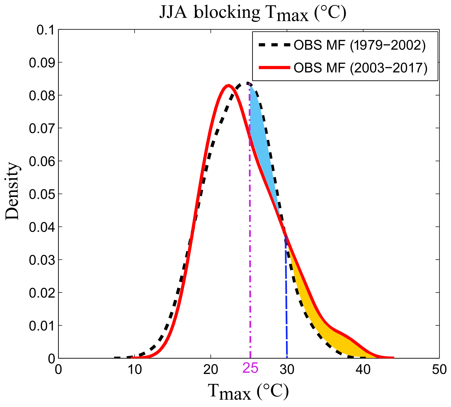
Figure 13PDF of the Tmax for the blocking regime. The dotted black line represents the past period from 1979 to 2002, and the solid red line reflects the current period from 2003 to 2017. The purple vertical segment represents the threshold of the SU, i.e. 25 ∘C. The blue vertical segment represents the temperature at which a frequency inversion occurs between the past period, with a higher frequency of temperatures between 25 and 30 ∘C (blue-coloured zone), and the current period, with a higher frequency of temperatures above 30 ∘C (orange-coloured zone).
6.1 Changes associated with large-scale dynamics
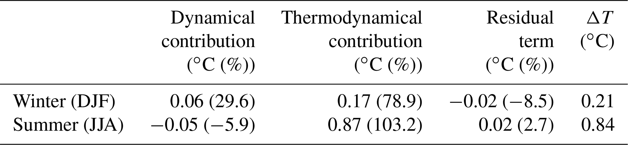
Dynamical changes are by definition related to large-scale atmospheric circulation changes. According to Vautard and Yiou (2009), changes in atmospheric circulation are the main drivers of surface weather patterns in winter. In the Paris area over the past 40 years, we have seen very few significant trends in temperature, relative humidity and precipitation during the winter season. Comparing the two periods, Table 3 shows that the temperature change is 4 times lower in winter (ΔT) than in summer. Changes in occurrence of winter regimes contribute to one-fourth of the observed change versus three-fourths for thermodynamic changes (Table 3). Indeed, in terms of dynamics, Yiou et al. (2018) detected significant trends in the stability of the circulation and the return period since the 1970s in winter; that is, winters tend to be similar to those already known, which increases the predictability of winter circulations. In Europe, Francis and Vavrus (2012) and Petoukhov et al. (2013) showed that the wave amplitude in winter is changing, particularly through a connection between the Arctic sea ice cover and the sinuosity of the jet stream which brings prolonged weather conditions enhances the probability for extreme weather as cold spells. These cold winters may be related to the acceleration of Arctic warming associated with ice retreat (Cohen et al., 2012, 2014; Tang et al., 2013; Vihma, 2014; Walsh, 2014; Zappa and Shepherd, 2017) by ice–albedo feedbacks (Screen and Simmonds, 2010). Recently, Kretschmer et al. (2018) showed that in recent decades, the stratospheric polar vortex has shifted to more frequent weak states, which may explain Eurasian cooling trends in northern winter. However, it remains controversial whether this European winter cooling could also be related to internal atmospheric variability (Sun et al., 2016), tropical trends (Palmer, 2014), Arctic trends (Cohen et al., 2014, 2012; Tang et al., 2013; Vihma, 2014; Walsh, 2014; Zappa and Shepherd, 2017) or a combination of all these variabilities. All of these processes appear to indicate that winter is marked by a stability of the circulation and that some observed trends, such as colder winters, appear to be related to modification of the atmospheric states themselves. This is why this study focuses on summer, when the changes are more significant and more related to thermodynamical processes (+103.2 %; Table 3).
Table 3Dynamical, thermodynamical and residual contributions of the temperature change (ΔT) in ∘C in winter (DJF) and in summer (JJA). Values in brackets give the ratio (in %) between the change components and the total change.
In spring, the T2 m and Tmax show the strongest increase compared to the other seasons, associated with a strong decrease in RH with punctually very cold Tmax and Tmin. According to Brunner et al. (2017), this increase in temperatures in spring associated with the presence of cold extremes is also related to the position of the blocking regime. The blocking regime induces cold conditions in winter but warm episodes in summer. In spring, the blocking position varies and impacts the distribution of extreme temperatures: cold waves in early spring are induced by a blocking position over the northeast Atlantic, while heat waves in late spring are associated with high-pressure centre over central Europe. Cassou and Cattiaux (2016) found a stretching of the summer period with an earlier onset of summer by ∼10 d between the 1960s and the 2000s. Moreover, Boé and Habets (2014) identified multidecadal variability with differences of river flow over France by up to 40 % in spring, which is linked with precipitation and temperature variabilities in France in spring by up to 30 % and 1 ∘C. Part of the increase in temperature observed in this study in the spring may therefore be associated with such multidecadal variability. Regarding precipitation in spring, the number of rainy days decreases, increasing (decreasing) dry (wet) periods but with more extremes of rainfall. This is consistent with the multidecadal variability of the precipitation described in Boé and Habets (2014) and Bonnet et al. (2017). These studies also suggest that these fluctuations are modulated by the Atlantic multidecadal variability (AMV) and that the North Pacific sea surface temperature, which exhibits variations in phase with the AMV, could also play a role in the multidecadal variability of the main French rivers, including the Seine river, which flows in Paris. As these strong multidecadal variations can seriously impact short-term trends, it is difficult to disentangle the trends we observed that are linked to natural variability from those associated with climate change.
Another aspect is that our study area is in a transition zone in terms of weather regimes. Summer regimes drive different climatic conditions at the European scale, but this distinction between regimes is not obvious when considering the Paris area, as already shown in Dione et al. (2017). For instance, the blocking regime is often considered as favouring heat waves, but in Paris it is characterized by cold extremes and mean values of T2 m, Tmax and Tmin closer to those of the regimes favouring colder conditions (Atlantic Ridge and NAO-). Such uncertainties are also found in precipitation, despite the use of different indices that allow the identification of the contribution of dynamics in the change of precipitation characteristics, as we did in Sect. 5.1. However, for more local studies, it would be interesting to carry out a sensitivity analysis on the size of the domain to be taken into account in the calculation of weather regimes, as was done by Jézéquel et al. (2018), to select the best analogues for studying specific events in western Europe. These results confirm that the dynamical component in climatic variability is very strong and must be taken into account, but that the thermodynamical component also plays a very important role.
6.2 Changes associated with thermodynamic and radiative processes
In summer, the temperature strongly interacts with the water cycle (Van Oldenborgh et al., 2009). Vautard and Yiou (2009) even show that in summer, atmospheric circulation changes are not the main factors of surface weather trends. Over Europe, Sousa et al. (2018) analysed different forcing mechanisms associated with blocking and Atlantic Ridge regimes, and they showed the importance of horizontal and vertical advection processes on summer temperature anomalies, especially diabatic heating processes. Although we found some changes in the occurrence of the four summer weather types, we also observed a strong evolution of the characteristics of each weather type. Table 3 shows that, in summer, the average temperature change is +0.84 ∘C between the two periods. If the thermodynamical component were the only contribution to change, this increase would have been 0.87 ∘C; conversely, if the dynamical component, i.e. the change in the occurrence, were the only contribution to the change, then we would observe a very slight decrease in temperature of approximately 0.05 ∘C.
In summer in the Paris area, T2 m, Tmax and Tmin increase strongly due to high changes in temperature extremes, while relative humidity decreases strongly with more dry anomalies. Vogel et al. (2017) show that the projected regional Tmax response in several midlatitude terrestrial regions can be divided into (i) the global mean warming trend and (ii) an additional temperature increase, strongly influenced by soil temperature feedbacks, linked to increasingly dry soil. They also show that this feedback is mostly related to multidecadal trends in soil moisture rather than its subseasonal or interannual variability and contributes to more than 70 % of the additional warming of regional hot extremes beyond global mean warming. At the Paris scale, surface layer drying is observed from spring to autumn, as shown in Fig. 14, by plotting the relationship between the seasonal surface temperature and specific humidity for each year; in this figure, colder colours are for older years and warmer colours for more recent years. In winter (Fig. 14a), there is a linear relationship between seasonal averaged T2 m and q2m, meaning that if the seasonal temperature of one winter is higher, there is also more humidity, and vice versa; we can even almost predict the value of seasonal humidity. It is not obvious that the more recent years have higher seasonal temperature for this season. For summer (Fig. 14c), as for winter, the temperature increase at the seasonal scale is not obvious. However, in recent years, from the end of 1990s, for a similar temperature as older years, the specific humidity shows lower average values. For spring (Fig. 14b), this lack of humidity starts slightly later, from 2000, but we can also see that more recent spring seasons present higher seasonal temperatures than older years, which amplifies the departure from the linear relationship. Theoretically, with global warming, the rise of temperature should be accompanied by an increase of the specific humidity for a given relative humidity. At Paris scale, the increase in the water retention capacity of the atmosphere (related to the increase in temperature) is not accompanied by an increase in the surface moisture (q), which leads to a decrease in surface relative humidity. There are several thermodynamical variables that take into account this co-dependence between temperature and relative humidity, which is often used to calculate heat stress (Buzan et al., 2015; Davies-Jones, 2008; Sherwood and Huber, 2010; Willett and Sherwood, 2012). We observed that the evolution on the specific humidity is similar to other coupled temperature and humidity variables, as the wet bulb temperature calculated via the formula of Davies-Jones (2008), meaning that the heat stress is constant (temperature increases but relative humidity decreases). In this paper, we use the specific humidity as one of these co-dependent variables. We then observe a surface drying, which can play a major role in the trend of other variables such as turbulent flows and thus can intensify or inhibit existing surface–atmosphere feedbacks. In Spain, Vicente-Serrano et al. (2014) observe the same trends with an increase in temperature leading to a decrease in relative humidity which is not accompanied by an increase in the surface water vapour content. They show that these trends are related to two constraints: (1) a terrestrial constraint related to a decrease of the precipitation and a decrease of soil moisture; and (2) an oceanic constraint related to a limitation in the advection of moisture from ocean surfaces.

Figure 14T2 m (∘C) – q (g kg−1) seasonal relationship in the Paris area from observations. Each point represents the seasonal average of 1 year.
Through the analysis of future projections, Cattiaux et al. (2015) show that the variation in diurnal temperatures increases in summer due to the decrease in surface evapotranspiration (linked to the European summer drying) and the reduction in cloud cover. This variation in diurnal temperatures is already observed in the Paris area, with an increase in Tmax above Tmin observed in spring and summer. In autumn (Fig. 14d), there are also lower humidity values for similar temperatures, but the signal is weaker than for summer. However, there is a striking increase in seasonal temperature for this season, associated with a nearly linear increase of humidity, unlike MAM. For the recent period, the warmer autumn seasonal averages associated with higher specific humidities are notably due to warmer and moister November months. At the seasonal timescale at the SIRTA supersite near Paris, Bastin et al. (2018) show that temperature variability is mainly controlled by surface fluxes.
At the Paris scale, in summer, the total rain amount increases but not significantly, and there is no change in specific humidity. The link between increasing temperatures (seen previously) and increasing precipitation has been highlighted by Rasmussen et al. (2017), who show, using a climatic simulation at convective-permitting resolution, the change in convective population in a warmer future climate, induced by both the increase of the CAPE but also of the CIN. Convection becomes more difficult to trigger, but once triggered, the energy available for convection is increased, favouring heavier precipitation. This means that weak to moderate convection will decrease and strong convection will increase in frequency in a future climate. This result therefore leads to a modification of the spatial and temporal occurrence of the precipitation. This may explain the bimodal structure displayed by the violin plot of humidity and precipitation in Fig. 9 for the Atlantic Low regime. The link between soil moisture and precipitation remains poorly understood. Indeed, Boé (2013) shows that in summer in France, previous soil moisture conditions could have a limited impact on precipitation through a modulation of large-scale circulation and the absolute effect of soil moisture on evapotranspiration is much larger than its effect on precipitation. Additionally, Vogel et al. (2017) show that changes in precipitation can also influence temperature and soil moisture variations.
Within the summer season, we observe very significant changes over 40 years independent of large-scale circulation, thus raising questions about the role played by local surface–atmosphere feedbacks in the context of warming. Temperatures in regimes favouring “cold conditions” warm up very clearly and even contribute for some years to very warm temperatures. Regimes favouring “hot conditions” continue to contribute very significantly to extreme heat events, such as heat waves. In particular, the Atlantic Low regime shows a very strong increase in the temperatures and a very strong decrease in the relative humidity, whereas precipitation and specific humidity show no trend but a change of their distribution. In a recent study, Bastin et al. (2019) analysed the spatial variability over Europe of the temperature thresholds over which the relative humidity starts to decrease using an integrated water vapour dataset from GPS stations. They suspect that the spatial variability of this threshold is strongly linked to local processes that drive moisture sources, in particular surface–atmosphere interactions and coastal/orographic circulations.
As shown by Zampieri et al. (2009) and Cattiaux et al. (2012), recent and future warming in Europe is incompatible with changes in atmospheric circulation alone, and surface–atmosphere processes are the mainly responsible for increasing temperature variability, especially summer temperatures. Furthermore, uncertainties in regional temperature projections can be linked to this long-term soil moisture–temperature feedback (Vogel et al., 2017).
6.3 Changes associated with local anthropogenic effects
Finally, some of the changes detected can be attributed to anthropogenic influence on land use, such as urbanization and irrigation. Changing a vegetated area to pavement strongly modifies the surface processes, with more runoff, less evapotranspiration and more heat. The enlargement of suburban areas affects the urban heat island processes. This is not the purpose of the paper, but it is an indispensable aspect to discuss in observed changes. Daniel (2017) compares different representations of urban areas within an atmospheric model with an explicit representation of the urban areas and concludes that cities can influence their environment on a regional scale. Thus, the largest French cities induce a warming trend of the temperature near the surface. This warming can reach up to 1.5 ∘C in summer Tmin in Paris. Thus, according to Wilcox et al. (2018), anthropogenic forcing may have slightly increased the risk of dry summers and greatly increased the risk of hot summers.
This study characterizes the main changes in trends and extremes of temperature, humidity and precipitation at the local scale in the Paris area, which is favoured by an urban heat island. The analysis was carried out annually and seasonally, including the effect of large-scale circulations in summer. The comparison of the observations with the ERA-I reanalysis shows that it strongly underestimates the temperatures (especially in summer) and overestimates the relative humidity. The local trends are not adequately characterized by ERA-I, especially for the climate extreme indices. This analysis thus confirms the importance of direct observation when dealing with the local scale. This study uses observation data from five stations in the Paris area starting from 1979 to characterize observed changes in temperatures, relative humidity and precipitation at different timescales. Although some trends are similar to the ones found at regional (Europe) or global scales, there are specific local patterns:
-
Tmax increases more strongly than Tmin at annual, seasonal (except SON) and summer scales.
-
There are few significant trends in winter, unlike in summer.
-
Summer temperatures increase due to a strong thermodynamical contribution.
-
In summer, the temperatures increase for the cooler weather regimes, especially NAO-, contributing to high temperatures. During this time, the hottest weather regimes keep warming even more. This is due to the advection of warming air masses from the ocean and a probable intensification of temperature in the air.
-
The relative humidity decreases considerably, especially in spring and summer. This is particularly true for the Atlantic Low weather regime in summer.
-
The specific humidity shows little or no trends, although it was expected to increase associated with warming and the proximity to the English Channel.
-
Rainfall has a high variability from one year to the next, but the trend, even if not truly significant, appears to be decreasing (except in summer). There appears to be a change in the precipitation regime with a less rainy winter, a generally drier spring with more intense rainfall and a wetter summer, one-third explained by a change in occurrence in summer weather regimes and two-thirds explained by a change in thermodynamic unrelated to circulation.
It is important to understand the physical processes behind these changes at the local scale and especially during the summer season, as they are likely to intensify or become inhibited with the current climate change. Some of these processes have been discussed in the previous section; however, there are several feedbacks that are still poorly understood in the context of global warming, particularly in such an urbanized area. As this very recent study by Schwingshackl et al. (2018) shows, it is crucial to take into account local and regional processes to properly assess interannual variability in temperature and future trends in temperature.
One of the perspectives of this study is to understand these current changes using the rather complete set of atmospheric observations from the supersite of Chiriaco et al. (2018), which has collected more than 50 meteorological and atmospheric parameters at hourly time steps since 2003 over the full boundary layer. The strong correlation between the stations as well as the average of the stations encourages us to use this dataset.
The meteorological station data used in this study are paid public data, but are accessible free of charge under a teaching-research license. The continuous time weather regimes data can be found via the A2C2 website at http://dods.lsce.ipsl.fr/dase/REGIMES/ (Yiou et al., 2008) last access: 15 January 2019. ERA-Interim data are available from the European Centre for Medium-Range Weather Forecasts (ECMWF). Finally, SAFRAN is available for research actions. You must make an access request here: http://mistrals.sedoo.fr/?editDatsId=47&datsId=47&project_name=HyMeX&q=safran (METEO-FRANCE, SIM reanalysis), last access: 15 January 2019.
A1 ERA-Interim
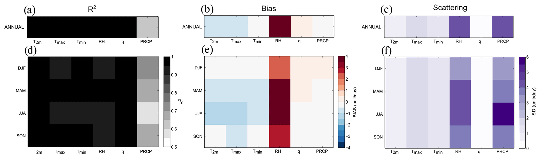
Figure A1Statistical comparison between daily ERA-I and daily MF observations for T2 m, Tmax, Tmin, RH and q (one column, one variable in each subfigure) and between daily SAFRAN and daily MF observations for PRCP (last column in each figure). (a–c) Annual statistical comparison and (d–f) seasonal statistical comparison. Panels (a) and (d) show R2, the correlation coefficient. Panels (b) and (e) show the bias (in units d−1). Panels (c) and (f) show scattering, the standard deviation from the diagonal.
The ERA-Interim (ERA-I) reanalysis developed by ECMWF is a global atmospheric reanalysis available from 1979 to today, every 6 h and at a spatial resolution of (Dee et al., 2011; Dee and Uppala, 2009; Simmons et al., 2014). The ERA-I dataset contains both analyses and forecasts. Unlike T2 m, which contains analyses four times per day (00:00, 06:00, 12:00 and 18:00 UTC), Tmax and Tmin series under ERA-I are built from daily forecasts. There are five time values per day: 00:00, 06:00, 12:00, 18:00, and 00:00 UTC, corresponding to the five forecasting steps (12, 18, 24, 30 and 36 h) starting at the reference time 12:00 UTC of the day before; thus, the daily value Tmax and Tmin of ERA-I are selected by selecting the maximum or minimum daily values from the five values available on the corresponding day. The configuration of the ERA-I grid imposes a grid point in the near centre of our study area, involving the presence of observation stations on four different ERA-I pixels (green square; Fig. 1). We performed a sensitivity analysis to compare each pixel to the average of the four pixels. The result shows that the differences between each pixel, as well as the average of the four pixels, are very weak for all considered variables. We only observed a slightly different variability for the northwestern pixel at the seasonal scale, with a slightly warmer and drier pixel for T2 m in winter and a little colder and slightly wetter pixel for T2 m and Tmax in the summer. This pixel is located closer to the English Channel (only 55 km), so it is more subject to oceanic conditions with milder winters and cooler summers. We chose to average the four pixels in order to obtain a spatial coverage including all the observation stations. The data of T2 m, Tmax, Tmin and RH are collected for the four ERA-I pixels (green square; Fig. 1) and then averaged to obtain a daily spatial average.
A2 SAFRAN
For precipitation, we use a meteorological analysis system called SAFRAN (Système d'Analyse Fournissant des Renseignements Adaptés à la Nivologie) (Durand et al., 1993) developed by the Centre National de Recherches Météorologiques et le Centre d'études de la Neige (CNRM/CEN). The main characteristic of SAFRAN is its treatment of a limited area divided into non-regular and climatologically homogeneous areas. As input, SAFRAN uses vertical profiles derived from the meteorological model as well as numerous sources of observations. The data are analysed by altitude range (300 m steps) via optimal interpolation (6 h time steps and 24 h time steps for precipitation). The analyses are then interpolated at the hourly time step; then, a spatial interpolation is performed to project the data on a regular grid. In output, the SAFRAN meteorological analysis system has a spatial resolution of 8 km × 8 km and an hourly temporal resolution. These data are available from 1958 to 2016. This study collects and averages 36 pixels, whose spatial coverage represents the “small Parisian crown” (orange in Fig. 1).
A3 Statistical comparisons
The daily average of the five Météo-France observation stations for T2 m, Tmax, Tmin, RH and q are compared to the daily average of the 4 pixels of ERA-I grid, which encompasses the MF stations (in green in Fig. 1). For precipitation, we compare the daily average of the four MF stations (without Trappes) with the daily average of the SAFRAN grid (in orange in Fig. 1). The statistical comparison uses the correlation coefficient, the bias and the standard deviation.
On an annual scale (Fig. A1a–c), all variables except precipitation show a very good correlation coefficient between observations and analysis (Fig. A1a). ERA-I underestimates T2 m, especially Tmax with −1 ∘C (Fig. A1b), and overestimates RH (about +4 %). The standard deviation from the diagonal is very small for temperatures and specific humidity but more significant for relative humidity (Fig. A1c). For precipitation, SAFRAN bias is very low (Fig. A1b) but probably due to compensatory errors, since the correlation coefficient is not very high and associated with a significant standard deviation (Fig. A1c).
At the seasonal scale (Fig. A2d–f), the correlation coefficient for temperatures and humidities is very good in all seasons but not for precipitation (Fig. A1d). This is certainly a signature of the very high variability of precipitation. The annual underestimate of temperature by ERA-I is the result of an underestimate of temperatures for all seasons. It is, however, more significant in summer, with −1.4 ∘C for Tmax and −1 ∘C for T2 m (Fig. A1e). This strong underestimation of ERA-I is also marked in spring and for Tmax in autumn (Fig. A1e). Several reasons explain this underestimation of ERA-I on the temperatures. First, the coverage taken into account of the ERA-I grid is greater than the “Parisian crown”. Second, for T2 m, the daily temperatures are averaged over the analyses performed every 6 h. Third, Tmax and Tmin are not analyses but daily forecasts. ERA-I overestimates relative humidity for all seasons, especially in MAM and JJA with values near 4 % (Fig. A1e). Moreover, the standard deviation from the diagonal is very strong (Fig. A1f). These are months with humidity coming from surface evaporation playing an important role in the total relative humidity amount. This overestimate by ERA-I suggests stronger latent heat flux in ERA-I than in observations. For rainfall, the SAFRAN bias is relatively low in all seasons (Fig. A1e), but summer has less correlation (Fig. A1d) and more scattering than other seasons (Fig. A1f). JJA corresponds to a period when precipitation is mostly convective and more locally and suddenly impacts the local measurements. The statistical evaluation at the daily timescale is thus very challenging. The statistical analysis of SAFRAN performed from the monthly accumulation gives better results, confirming that SAFRAN is an analysis module that represents the precipitation at the local scale rather well.
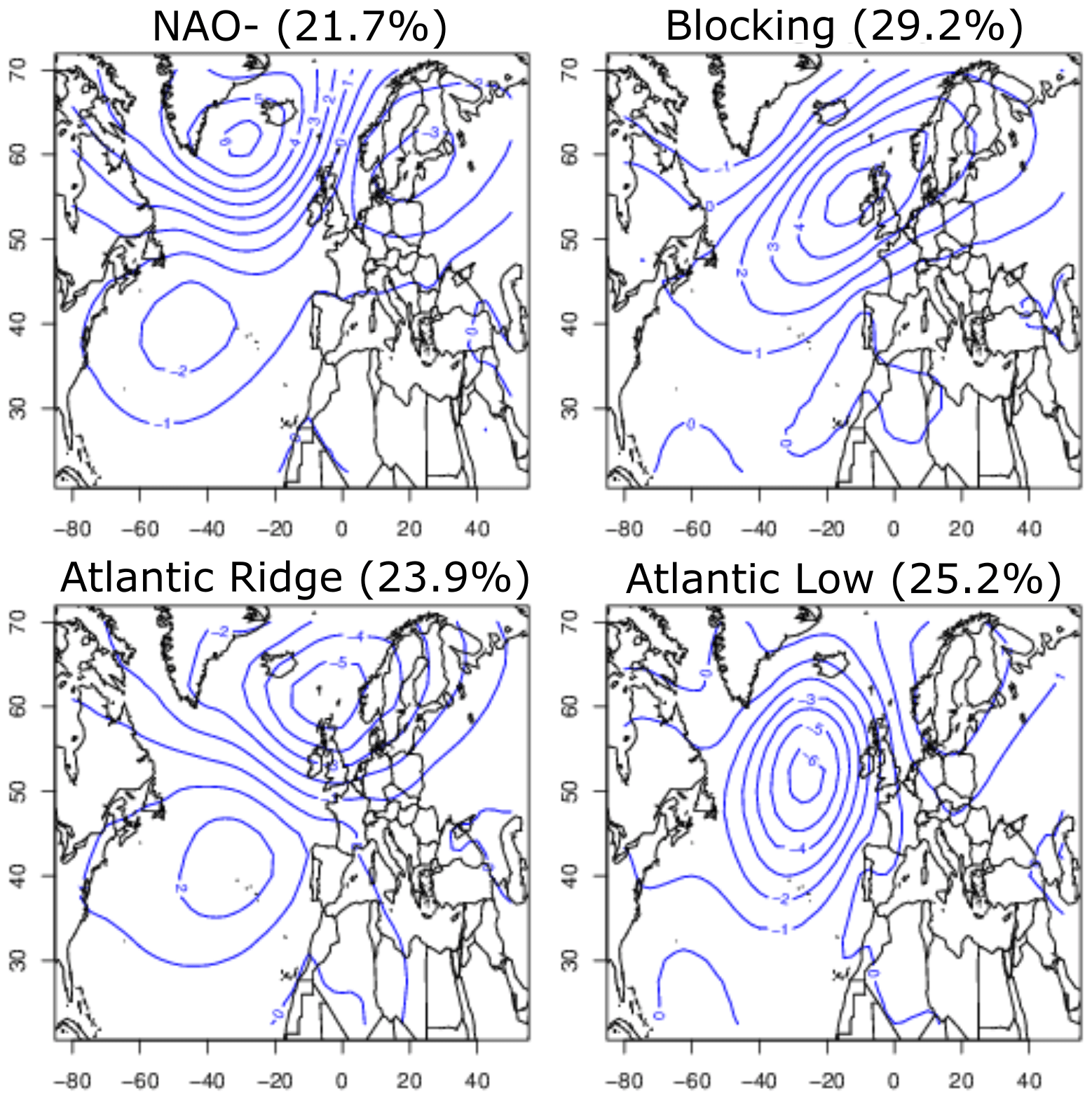
Figure B1North Atlantic summer weather regimes computed on the sea level pressure from National Centers for Environmental Prediction reanalysis based on reference periods from 1970 to 2010. The weather regimes were determined on seasonal anomalies of SLP. The isolines show SLP anomalies in hPa for NAO-, Atlantic Ridge, blocking and Atlantic Low. The average frequencies of the regimes over the 1979–2017 period are indicated by percent signs. The figure is from https://a2c2.lsce.ipsl.fr/index.php/deliverables, last access: 15 January 2019.
JR carried out the data analysis and prepared all the figures. JR, MC, SB and FH contributed to the data analysis and interpretation of results. JR wrote the manuscript with contributions from all co-authors.
The authors declare that they have no conflict of interest.
We would like to acknowledge Météo-France for the provision of observation measurements and the SAFRAN analysis. We also would like to acknowledge Pascal Yiou, who provided the weather regime classification via the project A2C2, supported by ERC grant 338965-A2C2. To process the data, this study benefited from the IPSL mesocenter ESPRI facility, which is supported by CNRS, UPMC, Labex L-IPSL, CNES and Ecole Polytechnique.
This research has been supported by the LABEX L-IPSL, funded by the French Agence Nationale de la Recherche, under the programme “Investissements d'Avenir” (grant no. ANR-10-LABX-18-01).
This paper was edited by Hang Su and reviewed by three anonymous referees.
Bastin, S., Chiriaco, M., and Drobinski, P.: Control of radiation and evaporation on temperature variability in a WRF regional climate simulation: comparison with colocated long term ground based observations near Paris, Clim. Dynam., 51, 985–1003, https://doi.org/10.1007/s00382-016-2974-1, 2018.
Bastin, S., Drobinski, P., Chiriaco, M., Bock, O., Roehrig, R., Gallardo, C., Conte, D., Dominguez-Alonso, M., Li, L., Lionello, P., and Parracho, A. C.: Impact of humidity biases on light precipitation occurrence: observations versus simulations, Atmos. Chem. Phys., 19, 1471–1490, https://doi.org/10.5194/acp-19-1471-2019, 2019.
Boé, J.: Modulation of soil moisture–precipitation interactions over France by large scale circulation, Clim. Dynam., 40, 875–892, https://doi.org/10.1007/s00382-012-1380-6, 2013.
Boé, J. and Habets, F.: Multi-decadal river flow variations in France, Hydrol. Earth Syst. Sci., 18, 691–708, https://doi.org/10.5194/hess-18-691-2014, 2014.
Bonnet, R., Boé, J., Dayon, G., and Martin, E.: Twentieth-Century Hydrometeorological Reconstructions to Study the Multidecadal Variations of the Water Cycle Over France, Water Resour. Res., 53, 8366–8382, https://doi.org/10.1002/2017WR020596, 2017.
Brunner, L., Hegerl, G. C., and Steiner, A. K.: Connecting Atmospheric Blocking to European Temperature Extremes in Spring, J. Clim., 30, 585–594, https://doi.org/10.1175/JCLI-D-16-0518.1, 2017.
Buzan, J. R., Oleson, K., and Huber, M.: Implementation and comparison of a suite of heat stress metrics within the Community Land Model version 4.5, Geosci. Model Dev., 8, 151–170, https://doi.org/10.5194/gmd-8-151-2015, 2015.
Cassano, J. J., Uotila, P., Lynch, A. H., and Cassano, E. N.: Predicted changes in synoptic forcing of net precipitation in large Arctic river basins during the 21st century, J. Geophys. Res.-Biogeo., 112, G04S49, https://doi.org/10.1029/2006JG000332, 2007.
Cassou, C. and Cattiaux, J.: Disruption of the European climate seasonal clock in a warming world, Nat. Clim. Change, 6, 589–594, https://doi.org/10.1038/nclimate2969, 2016.
Cassou, C., Terray, L., and Phillips, A. S.: Tropical Atlantic Influence on European Heat Waves, J. Clim., 18, 2805–2811, https://doi.org/10.1175/JCLI3506.1, 2005.
Cassou, C., Minvielle, M., Terray, L., and Périgaud, C.: A statistical–dynamical scheme for reconstructing ocean forcing in the Atlantic, Part I: weather regimes as predictors for ocean surface variables, Clim. Dynam., 36, 19–39, https://doi.org/10.1007/s00382-010-0781-7, 2011.
Cattiaux, J.: Extrêmes de température en Europe: mécanismes et réponses au changement climatique, Pd.D. thesis, Universite Pierre et Marie Curie (Paris 6), France, 244 pp., 2010.
Cattiaux, J., Yiou, P., and Vautard, R.: Dynamics of future seasonal temperature trends and extremes in Europe: a multi-model analysis from CMIP3, Clim. Dynam., 38, 1949–1964, https://doi.org/10.1007/s00382-011-1211-1, 2012.
Cattiaux, J., Douville, H., Schoetter, R., Parey, S., and Yiou, P.: Projected increase in diurnal and interdiurnal variations of European summer temperatures, Geophys. Res. Lett., 42, 899–907, https://doi.org/10.1002/2014GL062531, 2015.
Chiriaco, M., Bastin, S., Yiou, P., Haeffelin, M., Dupont, J.-C., and Stéfanon, M.: European heatwave in July 2006: Observations and modeling showing how local processes amplify conducive large-scale conditions, Geophys. Res. Lett., 41, 5644–5652, https://doi.org/10.1002/2014GL060205, 2014.
Chiriaco, M., Dupont, J.-C., Bastin, S., Badosa, J., Lopez, J., Haeffelin, M., Chepfer, H., and Guzman, R.: ReOBS: a new approach to synthesize long-term multi-variable dataset and application to the SIRTA supersite, Earth Syst. Sci. Data, 10, 919–940, https://doi.org/10.5194/essd-10-919-2018, 2018.
Cohen, J. L., Furtado, J. C., Barlow, M. A., Alexeev, V. A., and Cherry, J. E.: Arctic warming, increasing snow cover and widespread boreal winter cooling, Environ. Res. Lett., 7, 014007, https://doi.org/10.1088/1748-9326/7/1/014007, 2012.
Cohen, J. L., Screen, J. A., Furtado, J. C., Barlow, M., Whittleston, D., Coumou, D., Francis, J., Dethloff, K., Entekhabi, D., Overland, J., and Jones, J.: Recent Arctic amplification and extreme mid-latitude weather, Nat. Geosci., 7, 627–637, https://doi.org/10.1038/ngeo2234, 2014.
Dai, A., Fyfe, J. C., Xie, S.-P., and Dai, X.: Decadal modulation of global surface temperature by internal climate variability, Nat. Clim. Change, 5, 555–559, https://doi.org/10.1038/nclimate2605, 2015.
Daniel, M.: Villes, climat urbain et climat régional sur la France: étude par une approche de modélisation climatique couplée, Pd.D. thesis, Université Toulouse III-Paul Sabatier, France, 197 pp., 2017.
Davies-Jones, R.: An Efficient and Accurate Method for Computing the Wet-Bulb Temperature along Pseudoadiabats, Mon. Weather Rev., 136, 2764–2785, https://doi.org/10.1175/2007MWR2224.1, 2008.
Dee, D. P. and Uppala, S.: Variational bias correction of satellite radiance data in the ERA-Interim reanalysis, Q. J. R. Meteorol. Soc., 135, 1830–1841, https://doi.org/10.1002/qj.493, 2009.
Dee, D. P., Uppala, S. M., Simmons, A. J., Berrisford, P., Poli, P., Kobayashi, S., Andrae, U., Balmaseda, M. A., Balsamo, G., Bauer, P., Bechtold, P., Beljaars, A. C. M., van de Berg, L., Bidlot, J., Bormann, N., Delsol, C., Dragani, R., Fuentes, M., Geer, A. J., Haimberger, L., Healy, S. B., Hersbach, H., Hólm, E. V., Isaksen, L., Kållberg, P., Köhler, M., Matricardi, M., McNally, A. P., Monge-Sanz, B. M., Morcrette, J.-J., Park, B.-K., Peubey, C., de Rosnay, P., Tavolato, C., Thépaut, J.-N., and Vitart, F.: The ERA-Interim reanalysis: configuration and performance of the data assimilation system, Q. J. R. Meteorol. Soc., 137, 553–597, https://doi.org/10.1002/qj.828, 2011.
Dione, C., Lohou, F., Chiriaco, M., Lothon, M., Bastin, S., Baray, J.-L., Yiou, P., and Colomb, A.: The Influence of Synoptic Circulations and Local Processes on Temperature Anomalies at Three French Observatories, J. Appl. Meteorol. Climatol., 56, 141–158, https://doi.org/10.1175/JAMC-D-16-0113.1, 2017.
Donat, M. G. and Alexander, L. V.: The shifting probability distribution of global daytime and night-time temperatures, Geophys. Res. Lett., 39, L14707, https://doi.org/10.1029/2012GL052459, 2012.
Donat, M. G., Alexander, L. V., Yang, H., Durre, I., Vose, R., Dunn, R. J. H., Willett, K. M., Aguilar, E., Brunet, M., Caesar, J., Hewitson, B., Jack, C., Klein Tank, A. M. G., Kruger, A. C., Marengo, J., Peterson, T. C., Renom, M., Oria Rojas, C., Rusticucci, M., Salinger, J., Elrayah, A. S., Sekele, S. S., Srivastava, A. K., Trewin, B., Villarroel, C., Vincent, L. A., Zhai, P., Zhang, X., and Kitching, S.: Updated analyses of temperature and precipitation extreme indices since the beginning of the twentieth century: The HadEX2 dataset, J. Geophys. Res.-Atmos., 118, 2098–2118, https://doi.org/10.1002/jgrd.50150, 2013.
Dong, B., Sutton, R. T., and Shaffrey, L.: Understanding the rapid summer warming and changes in temperature extremes since the mid-1990s over Western Europe, Clim. Dynam., 48, 1537–1554, https://doi.org/10.1007/s00382-016-3158-8, 2017.
Durand, Y., Brun, E., Merindol, L., Guyomarc'h, G., Lesaffre, B., and Martin, E.: A meteorological estimation of relevant parameters for snow models, Ann. Glaciol., 18, 65–71, https://doi.org/10.3189/S0260305500011277, 1993.
Fischer, E. M., Rajczak, J., and Schär, C.: Changes in European summer temperature variability revisited, Geophys. Res. Lett., 39, L19702, https://doi.org/10.1029/2012GL052730, 2012.
Francis, J. A. and Vavrus, S. J.: Evidence linking Arctic amplification to extreme weather in mid-latitudes, Geophys. Res. Lett., 39, L06801, https://doi.org/10.1029/2012GL051000, 2012.
Haeffelin, M., Barthès, L., Bock, O., Boitel, C., Sony, S., Bouniol, D., Chepfer, H., Chiriaco, M., Cuesta, J., Delanoë, J., Drobinski, P., Dufresne, J.-L., Flamant, C., Grall, M., Hodzic, A., Hourdin, F., Lapouge, F., Lemaître, Y., Mathieu, A., Morille, Y., Naud, C., Noël, V., O'Hirok, W., Pelon, J., Pietras, C., Protat, A., Romand, B., Scialom, G., and Vautard, R.: SIRTA, a ground-based atmospheric observatory for cloud and aerosol research, Ann. Geophys., 23, 253–275, https://doi.org/10.5194/angeo-23-253-2005, 2005.
Horton, D. E., Johnson, N. C., Singh, D., Swain, D. L., Rajaratnam, B., and Diffenbaugh, N. S.: Contribution of changes in atmospheric circulation patterns to extreme temperature trends, Nature, 522, 465–469, https://doi.org/10.1038/nature14550, 2015.
Huntingford, C., Jones, P. D., Livina, V. N., Lenton, T. M., and Cox, P. M.: No increase in global temperature variability despite changing regional patterns, Nature, 500, 327–330, https://doi.org/10.1038/nature12310, 2013.
IPCC: Climate Change 2014: Synthesis Report, Contribution of Working Groups I, II and III to the Fifth Assessment Report of the Intergovernmental Panel on Climate Change, edited by: Core Writing Team, Pachauri, R. K., and Meyer, L. A., IPCC, Geneva, Switzerland, 151 pp., 2014.
Jézéquel, A., Yiou, P., and Radanovics, S.: Role of circulation in European heatwaves using flow analogues, Clim. Dynam., 50, 1145–1159, https://doi.org/10.1007/s00382-017-3667-0, 2018.
Karl, T. R., Nicholls, N., and Ghazi, A.: CLIVAR/GCOS/WMO Workshop on indices and indicators for climate extreme: Workshop Summary, in: Weather and Climate Extremes, edited by: Karl, T. R., Nicholls, N., and Ghazi, A., Springer, Dordrecht, 3–7, https://doi.org/10.1007/978-94-015-9265-9_2, 1999.
Kendall, M. G.: Rank correlation methods, Hafner Publishing Co., Oxford, England, 196 pp., 1955.
Kodra, E. and Ganguly, A. R.: Asymmetry of projected increases in extreme temperature distributions, Sci. Rep., 4, 5884, https://doi.org/10.1038/srep05884, 2014.
Kretschmer, M., Coumou, D., Agel, L., Barlow, M., Tziperman, E., and Cohen, J.: More-Persistent Weak Stratospheric Polar Vortex States Linked to Cold Extremes, B. Am. Meteorol. Soc., 99, 49–60, https://doi.org/10.1175/BAMS-D-16-0259.1, 2018.
Legras, B. and Ghil, M.: Persistent Anomalies, Blocking and Variations in Atmospheric Predictability, J. Atmos. Sci., 42, 433–471, 1985.
Lewis, S. C. and King, A. D.: Evolution of mean, variance and extremes in 21st century temperatures, Weather Clim. Extrem., 15, 1–10, https://doi.org/10.1016/j.wace.2016.11.002, 2017.
Mann, H. B.: Nonparametric Tests Against Trend, Econometrica, 13, 245–259, https://doi.org/10.2307/1907187, 1945.
McKinnon, K. A., Rhines, A., Tingley, M. P., and Huybers, P.: The changing shape of Northern Hemisphere summer temperature distributions, J. Geophys. Res.-Atmos., 121, 8849–8868, https://doi.org/10.1002/2016JD025292, 2016.
METEO-FRANCE: SIM reanalysis – SAFRAN (over FRANCE), available at: http://http://mistrals.sedoo.fr/?editDatsId=47&datsId=47&project_name=HyMeX&q=safran, last access: 23 October 2019.
Michelangeli, P.-A., Vautard, R., and Legras, B.: Weather Regimes: Recurrence and Quasi Stationarity, J. Atmos. Sci., 52, 1237–1256, 1995.
Miralles, D. G., Teuling, A. J., van Heerwaarden, C. C., and Vilà-Guerau de Arellano, J.: Mega-heatwave temperatures due to combined soil desiccation and atmospheric heat accumulation, Nat. Geosci., 7, 345–349, https://doi.org/10.1038/ngeo2141, 2014.
Palmer, T.: Record-breaking winters and global climate change, Science, 344, 803–804, https://doi.org/10.1126/science.1255147, 2014.
Peterson, T. C., Folland, C. K., Gruza, G., Hogg, W., and Mokssit, A.: Report on the Activities of the Working Group on Climate Change Detection and Related Rapporteurs, World Meteorological Organization, Geneve, Switzerland, 2001.
Petoukhov, V., Rahmstorf, S., Petri, S., and Schellnhuber, H. J.: Quasiresonant amplification of planetary waves and recent Northern Hemisphere weather extremes, P. Natl. Acad. Sci. USA, 110, 5336–5341, https://doi.org/10.1073/pnas.1222000110, 2013.
Quintana-Seguí, P., Le Moigne, P., Durand, Y., Martin, E., Habets, F., Baillon, M., Canellas, C., Franchisteguy, L., and Morel, S.: Analysis of Near-Surface Atmospheric Variables: Validation of the SAFRAN Analysis over France, J. Appl. Meteorol. Climatol., 47, 92–107, https://doi.org/10.1175/2007JAMC1636.1, 2008.
Rasmussen, K. L., Prein, A. F., Rasmussen, R. M., Ikeda, K., and Liu, C.: Changes in the convective population and thermodynamic environments in convection-permitting regional climate simulations over the United States, Clim. Dynam., 1–26 https://doi.org/10.1007/s00382-017-4000-7, 2017.
Reinhold, B. B. and Pierrehumbert, R. T.: Dynamics of Weather Regimes: Quasi-Stationary Waves and Blocking, Mon. Weather Rev., 110, 1105–1145, 1982.
Rhines, A. and Huybers, P.: Frequent summer temperature extremes reflect changes in the mean, not the variance, P. Natl. Acad. Sci. USA, 110, E546, https://doi.org/10.1073/pnas.1218748110, 2013.
Schwingshackl, C., Hirschi, M., and Seneviratne, S. I.: Global Contributions of Incoming Radiation and Land Surface Conditions to Maximum Near-Surface Air Temperature Variability and Trend, Geophys. Res. Lett., 45, 5034–5044, https://doi.org/10.1029/2018GL077794, 2018.
Screen, J. A.: The missing Northern European winter cooling response to Arctic sea ice loss, Nat. Commun., 8, 14603, https://doi.org/10.1038/ncomms14603, 2017.
Screen, J. A. and Simmonds, I.: The central role of diminishing sea ice in recent Arctic temperature amplification, Nature, 464, 1334–1337, https://doi.org/10.1038/nature09051, 2010.
Seneviratne, S. I., Corti, T., Davin, E. L., Hirschi, M., Jaeger, E. B., Lehner, I., Orlowsky, B., and Teuling, A. J.: Investigating soil moisture–climate interactions in a changing climate: A review, Earth-Sci. Rev., 99, 125–161, https://doi.org/10.1016/j.earscirev.2010.02.004, 2010.
Shepherd, T. G.: Atmospheric circulation as a source of uncertainty in climate change projections, Nat. Geosci., 7, 703–708, https://doi.org/10.1038/ngeo2253, 2014.
Sherwood, S. C. and Huber, M.: An adaptability limit to climate change due to heat stress, P. Natl. Acad. Sci. USA, 107, 9552–9555, https://doi.org/10.1073/pnas.0913352107, 2010.
Simmons, A. J., Poli, P., Dee, D. P., Berrisford, P., Hersbach, H., Kobayashi, S., and Peubey, C.: Estimating low-frequency variability and trends in atmospheric temperature using ERA-Interim: Atmospheric Temperature Variability and Trends using ERA-Interim, Q. J. R. Meteorol. Soc., 140, 329–353, https://doi.org/10.1002/qj.2317, 2014.
Sippel, S., Zscheischler, J., Heimann, M., Otto, F. E. L., Peters, J., and Mahecha, M. D.: Quantifying changes in climate variability and extremes: Pitfalls and their overcoming, Geophys. Res. Lett., 42, 9990–9998, https://doi.org/10.1002/2015GL066307, 2015.
Sousa, P. M., Trigo, R. M., Barriopedro, D., Soares, P. M. M., and Santos, J. A.: European temperature responses to blocking and ridge regional patterns, Clim. Dynam., 50, 457–477, https://doi.org/10.1007/s00382-017-3620-2, 2018.
Sun, L., Perlwitz, J., and Hoerling, M.: What caused the recent “Warm Arctic, Cold Continents” trend pattern in winter temperatures?, Geophys. Res. Lett., 43, 5345–5352, https://doi.org/10.1002/2016GL069024, 2016.
Tang, Q., Zhang, X., Yang, X., and Francis, J. A.: Cold winter extremes in northern continents linked to Arctic sea ice loss, Environ. Res. Lett., 8, 014036, https://doi.org/10.1088/1748-9326/8/1/014036, 2013.
Tingley, M. P. and Huybers, P.: Recent temperature extremes at high northern latitudes unprecedented in the past 600 years, Nature, 496, 201–205, https://doi.org/10.1038/nature11969, 2013.
Uotila, P., Lynch, A. H., Cassano, J. J., and Cullather, R. I.: Changes in Antarctic net precipitation in the 21st century based on Intergovernmental Panel on Climate Change (IPCC) model scenarios, J. Geophys. Res.-Atmos., 112, D10107, https://doi.org/10.1029/2006JD007482, 2007.
Van Oldenborgh, G. J., Drijfhout, S., van Ulde, A., Haarsma, R., Sterl, A., Severijns, C., Hazeleger, W., and Dijkstra, H.: Western Europe is warming much faster than expected, Clim. Past, 5, 1–12, https://doi.org/10.5194/cp-5-1-2009, 2009.
Vautard, R.: Multiple Weather Regimes over the North Atlantic: Analysis of Precursors and Successors, Mon. Weather Rev., 118, 2056–2081, 1990.
Vautard, R. and Yiou, P.: Control of recent European surface climate change by atmospheric flow, Geophys. Res. Lett., 36, L22702, https://doi.org/10.1029/2009GL040480, 2009.
Vautard, R., Christidis, N., Ciavarella, A. et al.: Evaluation of the HadGEM3-A simulations in view of detection and attribution of human influence on extreme events in Europe, Clim. Dynam., 52, 1187–1210, https://doi.org/10.1007/s00382-018-4183-6, 2019.
Vicente-Serrano, S. M., Azorin-Molina, C., Sanchez-Lorenzo, A., Morán-Tejeda, E., Lorenzo-Lacruz, J., Revuelto, J., López-Moreno, J. I., and Espejo, F.: Temporal evolution of surface humidity in Spain: recent trends and possible physical mechanisms, Clim. Dynam., 42, 2655–2674, https://doi.org/10.1007/s00382-013-1885-7, 2014.
Vihma, T.: Effects of Arctic Sea Ice Decline on Weather and Climate: A Review, Surv. Geophys., 35, 1175–1214, https://doi.org/10.1007/s10712-014-9284-0, 2014.
Vogel, M. M., Orth, R., Cheruy, F., Hagemann, S., Lorenz, R., van den Hurk, B. J. J. M., and Seneviratne, S. I.: Regional amplification of projected changes in extreme temperatures strongly controlled by soil moisture-temperature feedbacks, Geophys. Res. Lett., 44, 1511–1519, https://doi.org/10.1002/2016GL071235, 2017.
Walsh, J. E.: Intensified warming of the Arctic: Causes and impacts on middle latitudes, Glob. Planet. Change, 117, 52–63, https://doi.org/10.1016/j.gloplacha.2014.03.003, 2014.
Wilcox, L. J., Yiou, P., Hauser, M., Lott, F. C., van Oldenborgh, G. J., Colfescu, I., Dong, B., Hegerl, G., Shaffrey, L., and Sutton, R.: Multiple perspectives on the attribution of the extreme European summer of 2012 to climate change, Clim. Dynam., 50, 3537–3555, https://doi.org/10.1007/s00382-017-3822-7, 2018.
Willett, K. M. and Sherwood, S.: Exceedance of heat index thresholds for 15 regions under a warming climate using the wet-bulb globe temperature, Int. J. Climatol., 32, 161–177, https://doi.org/10.1002/joc.2257, 2012.
WMO: World Meteorological Organization: Measurement of precipitation, in: Guide to Meteorological Instruments and Methods of Observation, World Meteorological Organization, Geneva, chapt. 6, Switzerland, 186–219, 2014.
Xoplaki, E., Luterbacher, J., Paeth, H., Dietrich, D., Steiner, N., Grosjean, M., and Wanner, H.: European spring and autumn temperature variability and change of extremes over the last half millennium, Geophys. Res. Lett., 32, L15713, https://doi.org/10.1029/2005GL023424, 2005.
Yiou, P., Goubanova, K., Li, Z. X., and Nogaj, M.: Weather regime dependence of extreme value statistics for summer temperature and precipitation, Onlinear Process. Geophys. Eur. Geosci. Union EGU, 3, 365–378, https://doi.org/10.5194/npg-15-365-2008, 2008.
Yiou, P., Malamud, B. D., and Rust, H. W.: Preface “Extreme Events: Nonlinear Dynamics and Time Series Analysis”, Nonlin. Process. Geophys., 18, 895–897, https://doi.org/10.5194/npg-18-895-2011, 2011.
Yiou, P., Cattiaux, J., Ribes, A., Vautard, R., and Vrac, M.: Recent Trends in the Recurrence of North Atlantic Atmospheric Circulation Patterns, Complexity, 2018, 1–8, https://doi.org/10.1155/2018/3140915, 2018.
Zampieri, M., D'Andrea, F., Vautard, R., Ciais, P., de Noblet-Ducoudré, N., and Yiou, P.: Hot European Summers and the Role of Soil Moisture in the Propagation of Mediterranean Drought, J. Clim., 22, 4747–4758, https://doi.org/10.1175/2009JCLI2568.1, 2009.
Zappa, G. and Shepherd, T. G.: Storylines of Atmospheric Circulation Change for European Regional Climate Impact Assessment, J. Clim., 30, 6561–6577, https://doi.org/10.1175/JCLI-D-16-0807.1, 2017.
Zhang, X., Alexander, L., Hegerl, G. C., Jones, P., Tank, A. K., Peterson, T. C., Trewin, B., and Zwiers, F. W.: Indices for monitoring changes in extremes based on daily temperature and precipitation data: Indices for monitoring changes in extremes, Wiley Interdiscip, Rev. Clim. Change, 2, 851–870, https://doi.org/10.1002/wcc.147, 2011.
Zolina, O., Simmer, C., Gulev, S. K., and Kollet, S.: Changing structure of European precipitation: Longer wet periods leading to more abundant rainfalls, Geophys. Res. Lett., 37, L06704, https://doi.org/10.1029/2010GL042468, 2010.
- Abstract
- Introduction
- Data
- Methodology
- General results
- Focus on the summer season
- Discussion
- Conclusions
- Data availability
- Appendix A: Comparison of the local observation with the ERA-Interim reanalyses and SAFRAN analysis
- Appendix B: North Atlantic weather regimes in summer
- Author contributions
- Competing interests
- Acknowledgements
- Financial support
- Review statement
- References