How waviness in the circulation changes surface ozone: a viewpoint using local finite-amplitude wave activity

Local finite-amplitude wave activity (LWA) measures the waviness of the local flow. In this work we relate the anticyclonic part of LWA, AWA (anticyclonic wave activity), to surface ozone in summertime over the US on interannual to decadal timescales. Interannual covariance between AWA diagnosed from the European Centre for Medium-Range Weather Forecast Era-Interim reanalysis and ozone measured at EPA Clean Air Status and Trends Network (CASTNET) stations is analyzed using maximum covariance analysis (MCA). The first two modes in the MCA analysis explain 84 % of the covariance between the AWA and MDA8 (maximum daily 8 h average ozone), explaining 29 % and 14 % of the MDA8 ozone variance, respectively. Over most of the US we find a significant relationship between ozone at most locations and AWA over the analysis domain (24–53^∘ N and 130–65^∘ W) using a linear regression model. This relationship is diagnosed (i) using reanalysis meteorology and measured ozone from CASTNET, or (ii) using meteorology and ozone simulated by the Community Atmospheric Model version 4 with chemistry (CAM4-chem) within the Community Earth System Model (CESM1). Using the linear regression model we find that meteorological biases in AWA in CAM4-chem, as compared to the reanalysis meteorology, induce ozone changes between −4 and +8 ppb in CAM4-chem. Future changes (ca. 2100) in AWA are diagnosed in different climate change simulations in CAM4-chem, simulations which differ in their initial conditions and in one case differ in their reactive species emissions. All future simulations have enhanced AWA over the US, with the maximum enhancement in the southwest. As diagnosed using the linear regression model, the future change in AWA is predicted to cause a corresponding change in ozone ranging between −6 and 6 ppb. The location of this change depends on subtle features of the change in AWA. In a number of locations this change is consistent with the magnitude and the sign of the overall simulated future ozone change.

1 Introduction

Tropospheric ozone impacts human health (McKee, 1993), the environment (e.g., Arneth et al., 2010), and climate (IPCC, 2013). The purpose of this study is to examine whether local wave activity (LWA hereafter), a newly developed diagnostic of the waviness of the atmospheric flow, can be used over the continental US to (i) quantify present-day surface ozone variability and (ii) predict the extent that future (ca. 2100) changes in atmospheric circulation will impact the surface ozone concentration.

Previous studies have shown that surface ozone is correlated with local meteorological factors such as surface temperature (e.g., Brown-Steiner et al., 2015), frontal passages (e.g., Ordónez et al., 2005), and stagnation (e.g., Jacob and Winner, 2009; Sun et al., 2017), although Kerr and Waugh (2018) show only a weak relationship on daily timescales between ozone and stagnation. In many regions, surface temperature is the largest covariate of surface ozone (Porter et al., 2015; Oswald et al., 2015). However, in the northeast US extended stagnation episodes predict high-ozone events better than temperature alone (Sun et al., 2017). Shen et al. (2015) note the importance of both the local and regional meteorological scales (e.g., synoptic-scale circulations) in determining ozone variability. On the larger scales jet position (Barnes and Fiore, 2013), the 500 hPa geopotential height (Lin et al., 2014; Shen et al., 2015), the Bermuda high location (Shen et al., 2015), and the frequency of cyclone passages (e.g., Leibensperger et al., 2008) all have been shown to impact local meteorological conditions and ozone. Less is known about the relation between ozone and features of the general circulation (but see Young et al., 2017), although ozone has been related to various indexes of the circulation including the Pacific Decadal Oscillation (Oswald et al., 2015), the Quasi-Biennial Oscillation (Oswald et al., 2015), El Niño and Southern Oscillation (e.g., Shen and Mickley, 2017a; Xu et al., 2017), the Arctic Oscillation (e.g., Oswald et al., 2015; Hess and Lamarque, 2007), and variations in stratosphere–troposphere exchange (e.g., Hess and Zbinden, 2013; Hess et al., 2015). While large-scale variables do not outperform the local variables in terms of their predictive power for ozone (Oswald et al., 2015), the impact of climate change on large-scale features of the circulation is likely more robust than that on smaller scales, and in some cases large-scale changes in circulation can be inferred from general theoretical arguments.

In this study we explore a general way to explain ozone's variability in terms of large-scale synoptic conditions through the LWA of the mid-tropospheric flow. Derived from the divergence theorem, finite-amplitude wave activity (Nakamura and Zhu, 2010) mathematically relates large-scale wave dynamics to the atmospheric circulation (Nakamura and Solomon, 2011; Methven, 2013; Chen and Plumb, 2014; Lu et al., 2015). LWA generalizes the zonally averaged finite-amplitude wave activity to local longitudinally dependent scales. It can be used to differentiate longitudinally isolated events and to characterize local and regional weather (Huang and Nakamura, 2016). Shen and Mickley (2017b) note the connection between the eastward-propagating flux in wave activity associated with the Pacific extreme pattern and increased surface pressure, reduced precipitation, warmer temperatures, more frequent heat waves, and enhanced ozone over the eastern US. A diagnosis of LWA also provides a metric for the occurrence of blocking events, events associated with anomalous or extreme mid-latitude weather such as heat waves (Chen et al., 2015; Martineau et al., 2017), which have been associated with surface ozone extremes (e.g., Sun et al., 2017; Meehl et al., 2018; Phalitnonkiat et al., 2018). Since blocking events are related to the flux and convergence of LWA, the processes that control LWA may provide clues to how blocking will change in the future (Nakamura and Huang, 2018). Thus LWA potentially makes a good candidate for relating surface ozone to characteristics of the general circulation.

Climate change causes notable and well-documented changes in surface ozone through changes in chemistry and changes in circulation. Changes in atmospheric chemistry from increased temperature and water vapor can either increase or decrease surface ozone, depending on surface emissions. An increase in the strength of the Brewer–Dobson circulation is a robust feature of future simulations (Garcia and Randel, 2008), although it is unclear as to the extent to which the associated increase in the stratosphere–troposphere exchange of ozone extends to the surface (Collins et al., 2003). Evidence of zonally symmetric changes in the future mid-latitude circulation (e.g., the increase in the strength of the Brewer–Dobson circulation) is more robust than that of regional changes. However, the use of LWA to diagnose circulation changes emphasizes zonally asymmetric changes with associated regional impacts.

There is some evidence for a zonally asymmetric climate-induced shift in storm tracks. The CMIP5 models predict a poleward shift in the jet position in the North Atlantic (Barnes and Polvani, 2013) although the Pacific storm track shows little movement with climate change (Shaw et al., 2016). The northward shift in the North Atlantic jet will likely decrease ozone variability over the northeast US and change the relationship between temperature and ozone (Barnes and Fiore, 2013). These changes in the storm track may also be related to changes in summertime cyclone frequency, reported in some (e.g., Leibensperger et al., 2008; Turner et al., 2013) but not all studies (Lang and Waugh, 2011) over the US. Over Europe notable future changes are predicted (Masato et al., 2013) in summertime blocking events. These events with their accompanying atmospheric persistence and temperature extremes are also associated with pollution extremes. However, blocking events are rare over the US during the summer months. The North Atlantic subtropical anticyclone (commonly referred to as the Bermuda High, Davis et al., 1997) has shown a consistent tendency in future model simulations to intensify and move to the west (e.g., Li et al., 2012; Shaw and Voigt, 2015). Ozone over the eastern part of the US is sensitive to the position and the variability of the Atlantic subtropical anticyclone (Shen et al., 2015). Horton et al. (2014) predict an increase in air stagnation over the southwestern US in the future, consistent with an increase in the future anticyclonic circulation in the southwestern part of the country (Shaw and Voigt, 2015). However, on the whole relatively little is known about how future zonally asymmetric circulation changes will impact surface ozone on a regional scale.

Here we focus on the extent that LWA is related to surface ozone and use this to predict the impact of circulation changes on ozone in the present and future climates. The advantages of using LWA are that it (i) provides a concise metric of regional circulation and its changes, (ii) provides a metric for anomalous mid-latitude weather events which have been associated with high surface ozone concentrations, and (iii) is fundamentally related to the large-scale flow field through finite-amplitude wave activity. Our emphasis on LWA does not preclude the importance of local meteorological effects on ozone such as the impact of local cloudiness, temperature, boundary layer ventilation, and wind direction. Indeed, as discussed below, local temperature has generally more predictive power than LWA on ozone. However, while local changes in temperature, for example, are important and are indeed related to the circulation changes characterized by LWA, it is difficult to diagnose changes in circulation from local temperature alone. Moreover, the predictions of future regional changes in circulation, as characterized, by LWA are likely more robust than future predictions of more local changes in temperature. Section 2 introduces data and methods. In Sect. 3 we (i) explore the relationship between ozone and LWA in the present climate in model simulations and observations and (ii) apply a simple univariate linear regression model to predict the ozone change in the future due to the change in LWA. Discussion and conclusions are given in Sect. 4.

2 Data and methods

2.1 Local wave activity calculation

The wave activity is calculated following Chen et al. (2015). To calculate LWA, for a quantity q (in this study we use geopotential height at 500 hPa, Z₅₀₀) decreasing with latitude in the Northern Hemisphere, we first define the equivalent latitude ϕ_e(Q) (Eq. 1), in which S(Q) is the area bounded by the q=Q contour towards the north pole (see Fig. 1):

$$\begin{array}{}\text{(1)}& {\mathit{\varphi }}_{\mathrm{e}}\left(Q\right)=\arcsin \left[\mathrm{1}-{\displaystyle \frac{S\left(Q\right)}{\mathrm{2}\mathit{\pi }{a}^{\mathrm{2}}}}\right].\end{array}$$

Figure 1 Anticyclonic local finite-amplitude wave activity (red) and cyclonic local finite-amplitude wave activity (blue) for the GCM2000 simulation based on the 25-year GCM2000 JJA average 5850 m geopotential height at 500 hPa (black contour). The dashed contour represents the equivalent latitude for this contour. At the equivalent latitude the magnitude of the local wave activity varies with longitude in proportion to the displacement of the black contour from the dashed contour. The total LWA(λ, ϕ_e) is equal to the cyclonic wave activity minus the anticyclonic wave activity.

The area within the equivalent latitude circle is equal to the area within the q=Q contour. The cyclonic (southern) and anticyclonic (northern) LWA at longitude λ and latitude ϕ_e can be defined as

$$\begin{array}{}\text{(2)}& \begin{array}{rl}& A_{\mathrm{C}}\left(\mathit{\lambda },{\mathit{\varphi }}_{\mathrm{e}}\right)={\displaystyle \frac{a}{\cos {\mathit{\varphi }}_{\mathrm{e}}}}{\int }_{\widehat{q}\le \mathrm{0},\mathit{\varphi }\le {\mathit{\varphi }}_{\mathrm{e}}\left(Q\right),\mathit{\lambda }=\mathrm{const}}\widehat{q}\cos \mathit{\varphi }\mathrm{d}\mathit{\varphi }\\ & A_{\mathrm{A}}\left(\mathit{\lambda },{\mathit{\varphi }}_{\mathrm{e}}\right)={\displaystyle \frac{a}{\cos {\mathit{\varphi }}_{\mathrm{e}}}}{\int }_{\widehat{q}\ge \mathrm{0},\mathit{\varphi }\ge {\mathit{\varphi }}_{\mathrm{e}}\left(Q\right),\mathit{\lambda }=\mathrm{const}}\widehat{q}\cos \mathit{\varphi }\mathrm{d}\mathit{\varphi },\end{array}\end{array}$$

where $\widehat{q}=q-Q$ (see Fig. 1). Thus, the cyclonic and anticyclonic LWA is defined by integrating the eddy term ($\widehat{q}$) southward and northward, respectively. The total LWA (A_T) is defined as in Huang and Nakamura (2016):

$$\begin{array}{}\text{(3)}& A_{\mathrm{T}}\left(\mathit{\lambda },{\mathit{\varphi }}_{\mathrm{e}}\right)=A_{\mathrm{C}}-A_{\mathrm{A}}.\end{array}$$

As defined in Eq. (2), A_C≤0 in the Northern Hemisphere, representing the cyclonic wave activity to the south of the equivalent latitude ϕ_e, and A_A≥0, representing the anticyclonic wave activity to the north. This formulation can be used to quantify the waviness in the time mean field as in Fig. 1 as well as in the synoptically varying daily field. More details on LWA theory and derivation can be found in Chen et al. (2015) and Huang and Nakamura (2016). Because the anticyclonic wave activity contributes to most of the total LWA over the continental US (Fig. 2) for simplicity and significance we relate the ozone concentration to anticyclonic wave activity (AWA) in the results below (the use of AWA gives similar results to using LWA). In addition, AWA is associated with high-pressure systems which oftentimes relate to high-ozone events.

Figure 2 JJA climatology of daily averaged wave activity in color shades (10⁸ m²). Anticyclonic local wave activity (a), cyclonic local wave activity (c), and the magnitude of total local wave activity (e) with 500 hPa geopotential height (contour, in m) for JJA 1979–2014 over the study region calculated from ERA-Interim reanalysis data. Climatology of anticyclonic local wave activity (b), cyclonic local wave activity (d), and the magnitude of total local wave activity (f) with 500 hPa geopotential height (contour, in m) for JJA 2006–2025 over the study region calculated from the GCM2000 simulation.

2.2 Measured and simulated data

The extent to which AWA can explain surface ozone variations is examined during the present day in both measured and simulated data during the summer months. We analyze the measured and simulated relationship between AWA and surface ozone concentrations in a study region defined as the region between 24–53^∘ N and 130–65^∘ W (see Fig. 2). This region, covering the continental US, is large enough to quantify the impact of non-local changes in AWA on surface ozone over the US, but not so large as to measure the impact of more distant teleconnection patterns. For the measured relationship we relate surface ozone concentrations measured at EPA Clean Air Status and Trends Network (CASTNET) sites to the AWA derived from meteorological reanalysis. The simulated relationship between AWA and ozone is derived using the Community Atmospheric Model version 4 with chemistry (CAM4-chem) in the Community Earth System Model (CESM1). The simulated future changes in AWA (ca. 2100) are then used to predict future changes in ozone due to future circulation change.

The measured relationship between AWA and ozone is analyzed for the summer months (June, July, August: JJA hereafter) for the period of 1994–2013. The measured surface ozone is taken from 49 CASTNET sites (see Fig. 3). At many measurement sites a decreasing trend is found in ozone during this time period (e.g., Cooper et al., 2014). Therefore, we split the study period into two equal length periods and remove the 21 d smoothed JJA seasonal cycle for each sub-period. The procedure produces a quasi-stationary time series for ozone at each site. In all cases we relate the maximum daily 8 h average ozone (MDA8 hereafter) to the wave activity. When analyzing the measured relationship between ozone and AWA, 500 hPa geopotential height from the European Centre for Medium-Range Weather Forecasts Era-Interim dataset (Dee et al., 2011) is used to compute AWA over the study region for the period of 1994–2013.

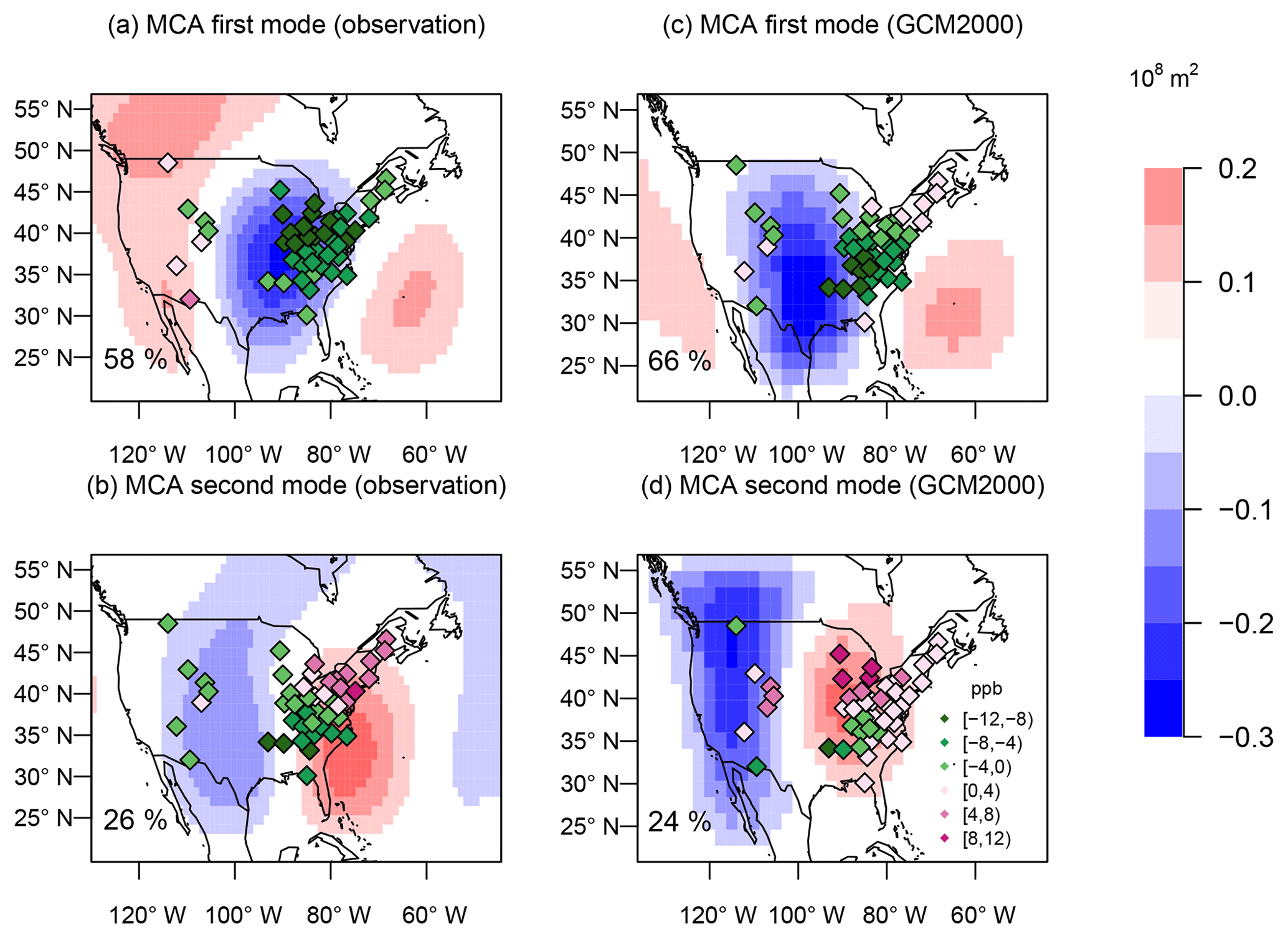
Figure 3 Spatial patterns of JJA AWA (color shades; in 10⁸ m²) and MDA8 ozone (colored diamonds; in ppb) from the maximum covariance analysis of AWA within the analysis domain and ozone at the CASTNET stations. The first mode (a) and the second mode (b) are from ERA-Interim meteorology and measured ozone at the CASTNET sites. Panels (c, d) are as in panels (a, b), except from the GCM2000 simulation of AWA and ozone at grid points closest to the CASTNET sites. The percent variance explained by each mode is given in the lower-left corner of each panel.

The Community Atmospheric Model version 4 (CAM4-chem) of the Community Earth System Model (CESM1) is used to simulate the relationship between ozone and AWA over the study region. CAM4-chem is described in Lamarque et al. (2012). CAM4-chem includes an extensive tropospheric chemistry scheme based on Emmons et al. (2010), with an extension to include stratospheric chemistry (see Tilmes et al., 2016). Reactions include gas phase, photolysis, and heterogenous reactions in both the stratosphere and troposphere. The simulated trend and magnitude of surface ozone in CAM4-chem has been largely improved compared to the earlier versions of the model because of the updates in the chemistry scheme, dry deposition rates, and radiation and optics due to a new treatment of aerosols (Tilmes et al., 2016). The resolution in the simulations analyzed below is 1.9^∘ latitude × 2.5^∘ longitude, with a model top of approximately ∼40 km.

Three ensemble members (different in their initial conditions) of the CESM1 CAM4-chem (REFC2) were run from 1960 to 2100 using the Climate Chemistry-Climate Model Initiative (CCMI) protocol. This protocol follows the RCP6 (Representative Concentration Pathway 6) scenario (Tilmes et al., 2016) for ozone and aerosol precursor emissions and mixing ratios for carbon dioxide, methane, and nitrous oxide (Table 1). CCMI is coordinated by the International Global Atmospheric Chemistry and Stratospheric Processes for the evaluation and intercomparison of chemistry–climate models, with the participation of many fully coupled chemistry–climate models (Eyring et al., 2013).

Table 1 CAM4-chem simulations used in this study.

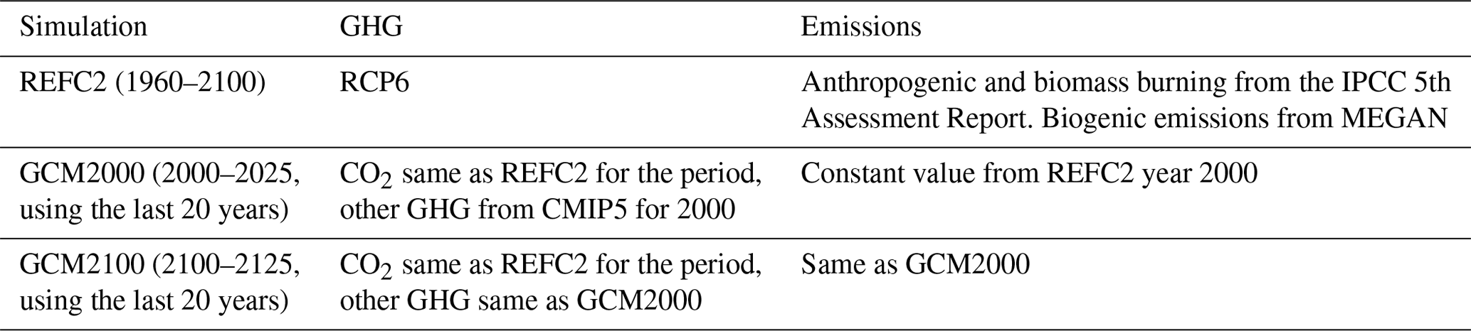
In addition to these three ensemble simulations we perform two climate-change-only simulations in order to isolate the impact of climate change on ozone (see Table 1): a present-day (the GCM2000 simulation) and a future simulation (the GCM2100 simulation). These simulations are branched off of the first ensemble member of the CESM1 CAM4-chem REFC2 simulation, one in 2000 and one in 2100, respectively. In both the GCM2000 and GCM2100 simulations, the emissions of all species including biogenic emissions and the concentrations of long-lived species (including CH₄) are kept constant at the 2000 level. In the present-day simulation, the atmospheric CO₂ was set at 369 ppm, representative of conditions ca. 2000, while in the future simulation CO₂ was set at 669 ppm, representative of conditions in 2100 following the RCP6 scenario. In the GCM2000 and GCM2100 simulations the simulation period is 26 years, with the last 20 years (2006–2025 or 2106–2125) used for the analysis. The average temperature change over the continental US between the GCM2100 simulation and the GCM2000 simulation is 2.1 ^∘C, smaller than the 2.8 ^∘C computed using the parent CCMI REFC2 simulations. This is likely due to the fact that the aerosol emissions are held constant at the 2000 levels in both the GCM2100 and GCM2000 simulations. The simulations are summarized in Table 1. Further analysis of these simulations is given in Phalitnonkiat et al. (2018). In this analysis both the MDA8 ozone and AWA time series are detrended by removing the 21 d smoothed JJA seasonal cycle.

2.3 Maximum covariance analysis

Maximum covariance analysis (MCA) (Wilks, 2011) finds the patterns in two spatially and temporally varying fields that explain the maximum fraction of covariance between them. We use MCA to find the overall relationship between ozone and AWA over the study region. Explicitly, the steps of calculating the MCA are as follows: (i) compute the covariance matrix for ozone and AWA over the considered domain and (ii) perform singular value decomposition (SVD) on the covariance matrix and obtain the modes that both dominate the ozone and AWA time series and strongly correlate with one another (resulting in the maximum covariance between the two time series).

2.4 The univariate linear regression model

A univariate linear regression model is used to quantify the relationship between ozone at individual points and AWA within the study region. The linear relationship between changes (in time) of deseasonalized ozone at a point (i₀, j₀) and changes in deseasonalized wave activity at another point (i, j) can be simply expressed as the slope of ozone with respect to wave activity (ppb m⁻²)($S_{i_{\mathrm{0}},j_{\mathrm{0}}(i,j)}$).

Summing over all points within the study region gives the projection (denoted by $p_{i_{\mathrm{0}},j_{\mathrm{0}}}$ (ppb)) of AWA on S. Thus $p_{i_{\mathrm{0}},j_{\mathrm{0}}}$ is calculated as follows:

$$\begin{array}{}\text{(4)}& p_{i_{\mathrm{0}},j_{\mathrm{0}}}=\mathbf{AWA}\cdot {\mathbf{S}}_{i_{\mathrm{0}},j_{\mathrm{0}}}=\sum _j\sum _i\mathbf{AWA}(i,j)\times {\mathbf{S}}_{i_{\mathrm{0}},j_{\mathrm{0}}}(i,j).\end{array}$$

The advantage of calculating the projection value p is that it measures in a single variable the similarity between the AWA and the ozone sensitivity to AWA, incorporating the regional impact of AWA on ozone. However, the projection in Eq. (4) can result in an overprediction of the contribution of AWA to ozone as the summation in Eq. (4) is not over statistically independent points. Therefore, to correct for this we build a linear regression model where we relate ${{\mathrm{O}}_{\mathrm{3}}}_{i_{\mathrm{0}},j_{\mathrm{0}}}$(t) to $p_{i_{\mathrm{0}},j_{\mathrm{0}}}$(t) through the linear regression coefficients ${\mathit{\alpha }}_{i_{\mathrm{0}},j_{\mathrm{0}}}$ and ${\mathit{\beta }}_{i_{\mathrm{0}},j_{\mathrm{0}}}$, where β is a measure of the overall sensitivity of ozone to AWA, and α gives the ozone background concentration:

$$\begin{array}{}\text{(5)}& {O_{\mathrm{3}}}_{i_{\mathrm{0}},j_{\mathrm{0}}}={\mathit{\beta }}_{i_{\mathrm{0}},j_{\mathrm{0}}}\times p_{i_{\mathrm{0}},j_{\mathrm{0}}}+{\mathit{\alpha }}_{i_{\mathrm{0}},j_{\mathrm{0}}}.\end{array}$$

On the daily timescale the relation between ozone and the projection value is quite noisy. Therefore, to reduce the noise we only apply Eq. (5) on an interannual timescale. Specifically we relate the interannual changes in ozone averaged over JJA to interannual changes in the JJA projection value. In turn the JJA averaged projection value (p) is calculated from the JJA averaged AWA multiplied by the slope (S) (Eq. 4). However, the slope (S) is noisy when calculated from interannual variations as we only have 20 years of data at our disposal. Thus we calculate S using daily variations of ozone and wave activity. In summary, the projection value for each year (Eq. 4) is calculated using the JJA averaged wave activity for each year but with S determined from daily variations.

In our analysis below we ascribe the change in ozone due to the change in AWA as

$$\begin{array}{}\text{(6)}& \mathrm{\Delta }{O}_{\mathrm{3}}=\mathit{\beta }\left[\left(\mathrm{\Delta }\mathbf{AWA}\right)\cdot \mathbf{S}\right].\end{array}$$

We apply this equation to (i) calculate the ozone bias that can be traced to differences in the AWA between the GCM2000 simulation and the ERA-Interim reanalysis and to (ii) calculate the ozone change that can be traced to future changes in the AWA. In both these cases we compute the climatological change in AWA, project it onto S, and multiply it by the slope β. In both cases we assume that S and β remain constant. For example, in the future we assume ozone responds to changes in the future AWA as it would respond to those same AWA changes in the present climate. The fact that β does not significantly change in the future is confirmed by an analysis of the GCM2100 simulation (see Sect. 3.3.2). Note that β (and S) can be derived from the GCM2000 simulation at all points or from the measurements at CASTNET sites. We will refer to these different estimates of ΔO₃ as the simulation-derived or measurement-derived ΔO₃.

3 Results

The climatological wave activity over the study region in the ERA-Interim reanalysis and in the GCM2000 simulation is given in Sect. 3.1, while the relation between variability in AWA and ozone is given in Sect. 3.2 using MCA. Section 3.3 analyzes the extent to which we can explain interannual changes in ozone from changes in AWA using the univariate linear regression model. This model is then used to explain the extent to which AWA differences between the GCM2000 simulation and the ERA-Interim reanalysis result in differences in the ozone distribution, and it explains the extent to which AWA differences between the GCM2100 simulation and the GCM2000 simulation result in ozone differences.

3.1 Climatological mean wave activity

Positive AWA anomalies are associated with 500 hPa ridges and cyclonic wave activity (CWA hereafter) anomalies with 500 hPa troughs (Fig. 2). The mean JJA LWA over the US in both the ERA-Interim reanalysis and the GCM2000 simulation is dominated by the anticyclonic component. In both datasets AWA anomalies are centered over the southwestern US with cyclonic wave activity mostly confined to the northeast and northwest of the study region. In each dataset, LWA (Fig. 2e,f) and AWA (Fig. 2a,b) are similar over the domain. While the GCM2000 simulation has a very dominant AWA maximum centered over the southwestern US, the ERA-Interim reanalysis has two maxima of approximately equal strength: one centered over the southwestern US and the other centered near 30–35^∘ N on the eastern border of the domain. The southwestern AWA maxima in the ERA-Interim reanalysis are much weaker than in the GCM2000 analysis. The simulated and reanalyzed LWA differences could be due to model bias or due to long timescale internal variability (e.g., Deser et al., 2012).

3.2 Maximum covariance analysis

MCA is used to examine the overall pattern of covariance between ozone and AWA (Fig. 3) as derived from measurements and from the GCM2000 simulation. In one case ozone is taken from the measurements at CASTNET sites while AWA is calculated from ERA-Interim reanalysis; in the other case both ozone and AWA are taken from the GCM2000 simulation, where ozone is sampled at the CASTNET sites. This analysis emphasizes the eastern US due to the high density of CASTNET stations there.

The first two modes identified in the MCA analysis derived from measurements (Fig. 3a, b) explain 84 % of their covariance, with the first mode explaining 58 % of the covariance followed by 26 % explained by the second mode (Fig. 3). The first mode consists of a positive anomaly of AWA off the eastern coast of the US and Canada, a negative AWA anomaly centered southwest of the Great Lakes, and a positive AWA anomaly in the western portion of the US. In the eastern third of the country the ozone anomaly is negative (up to −12 ppb). In the second mode a strong positive AWA anomaly is located on the eastern coast of the US, with a negative AWA anomaly over the center of the country. In the second mode the ozone anomalies range from strongly positive over the northeast US (up to 9 ppb) to negative over the southeast US (up to −10 ppb). If one uses the 500 hPa (Z₅₀₀) geopotential heights instead of AWA in this analysis (Fig. S1 in the Supplement) one obtains very similar results with small displacements in the Z₅₀₀ anomaly compared with the AWA anomaly.

The ozone anomalies identified here in the first two MCA modes are consistent with the leading two empirical orthogonal functions (EOFs) of ozone over the eastern US identified in Shen et al. (2015). Similar to our results, the first ozone EOF identified in Shen et al. (2015) has a negative ozone anomaly throughout the eastern US with the largest negative anomalies near 45^∘ N, while the second EOF has a positive ozone anomaly over the northeast US with negative anomalies over the southeast US and the Gulf Coast. Moreover, the correlation between the first two ozone EOFs and geopotential height in Shen et al. (2015) is consistent with the wave activity (or geopotential height) identified here in the first two modes of the MCA analysis. It is worth stressing that while the results in Shen et al. (2015) were obtained by first finding the leading EOFs of ozone, then correlating these EOFs with the geopotential height, the MCA methodology picks out the ozone and AWA (or geopotential height) anomalies in one procedure, with the first mode explaining 29 % of the total MDA8 ozone variance and the second mode explaining 14 % of the total ozone variance. Shen et al. (2015) attribute the first mode of the MCA to the impact of low-pressure systems crossing the eastern US and associate the second with the westward expansion of the North Atlantic subtropical anticyclone. A westward expansion of this anticyclone results in a negative ozone anomaly in the US Gulf states as ozone depleted air is advected inland from the Gulf Coast, but it results in a positive ozone anomaly in the northeastern US due to the advection of polluted mid-western air around the anticyclone to the northeast.

Similar to the results derived from measurements, the first simulated MCA mode explains 66 % of the total covariance, with the second mode explaining 24 % (Fig. 3c, d). For the total ozone variance, the first MCA mode explains 26 %, and the second MCA mode explains 18 %. The AWA in the first simulated mode differs only slightly from that in the reanalysis. The simulated AWA negative anomaly over the continental US is displaced slightly to the west of that from the ERA-Interim reanalysis. As a result, in the simulation the northeastern US is not subject to the cyclonic flow associated with the first observed mode, and consequently the simulated ozone anomalies over the very northeastern US are positive, not negative as in the observations. The second simulated mode differs more substantially from that observed with both the positive and negative AWA anomalies displaced substantially to the west (Fig. 3b, d) and with weak positive ozone anomalies extending from the northeast US south to Florida along the Atlantic seaboard. In contrast to the observations, the positive AWA anomaly in the second simulated mode is not correctly placed to advect high pollutant concentrations into the northeast US from the Ohio valley. In addition, the simulated negative ozone anomalies in the southeastern US attributed to transport of low-ozone air from the Gulf of Mexico are less extensive than measured.

The discrepancy between the observationally based and simulated MCA modes may, at least in part, stem from the simulation of the North Atlantic subtropical anticyclone (Fig. 4). In the ERA-Interim reanalysis the center of this anticyclone is located to the southeast of the simulated position, and the simulated low-pressure trough along the southeastern coast is not evident (Fig. 4). On the other hand, the western extension of the Atlantic anticyclone into the southeastern US in the reanalysis and the simulation are similar. The longitudinal variability of the position of this anticyclone is greater in the reanalysis than in the simulation, most likely leading to a larger range of impacts on continental ozone. Consistent with these differences, the MCA modes derived from the observations have rather strong associated ozone anomalies in the northeast US (strongly negative in the first mode and strongly positive in the second mode) while in the simulation these ozone variations are notably weaker. Phalitnonkiat et al. (2018) attribute the rather poor simulation of the temperature–ozone correlation in the northeastern US to the poor simulation of the Atlantic anticyclone while Zhu and Liang (2013) note deficiencies, in general, in the ability of general circulation models to simulate this subtropical high.

Figure 4 JJA 20-year average streamfunction (10⁶ m² s⁻¹) at 850 hPa for ERA-Interim reanalysis (shade), GCM2000 simulation (black contour), and GCM2100 simulation (gray contour).

3.3 Univariate regression analysis

At any point, the overall change in ozone attributed to changes in AWA is proportional to the change in AWA projected onto the regression coefficients (ppb m⁻²) calculated for that point (Eq. 6). The regression coefficients (ppb m⁻²) obtained between the ERA-Interim reanalysis (GCM2000 simulation) and measured ozone (simulated ozone) show strong, non-local, and significant relationships between AWA and ozone at all sites examined. For all sites the regression coefficient is positive at the site itself. The measurement-derived and simulation-derived regression coefficients are in general agreement, although some differences in magnitude and location do occur. We return to these regression coefficients when we examine future ozone changes in Sect. 3.3.2.

At most CASTNET sites, and throughout most of the simulated domain, interannual changes in AWA explain a statistically significant fraction of the interannual MDA8 ozone variability as determined by the linear regression equation (Eq. 5) (Fig. 5). Changes in AWA explain very little of the simulated ozone variability along the West Coast of the US and over the northeast US. In the western US it is possible that including changes in AWA outside the study region would hold more explanatory power. Note that in contrast to the simulation, the measurement-derived regression analysis explains a considerable fraction of the measured ozone variability over the northeastern US. A likely explanation is that over the northeast US the simulated variability (e.g., as captured by the MCA modes) is smaller than that measured and thus likely harder to capture.

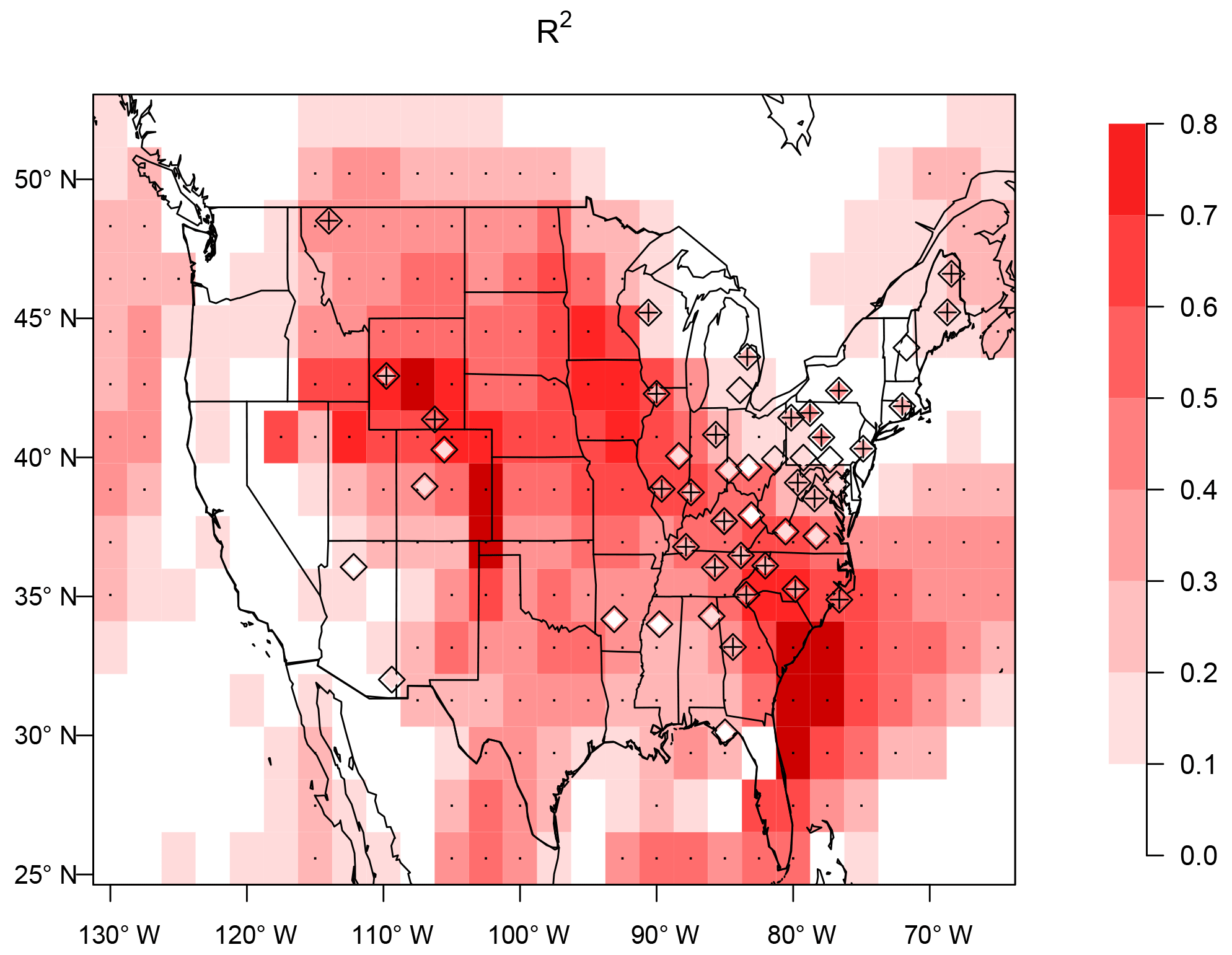
Figure 5 Interannual variance of MDA8 ozone explained (R²) by the linear regression model (Eq. 5) using the AWA projection value (Eq. 4) as the explanatory variable. Simulated variance is represented in shades (as derived from simulated ozone and AWA in the GCM2000 simulation) and measured variance is shown in diamonds (as derived from measured ozone at CASTNET sites and the ERA-Interim meteorology). Plus signs and stippling represent where R² is significant (at the 5 % significance level) at CASTNET sites and model grids, respectively.

It is equally possible to build a regression equation based simply on geopotential heights instead of wave activity. The variance of surface ozone explained within the study area tends to be somewhat higher than the variance explained using AWA (Fig. S3a), notably in the northeast US. However, it is important to note that wave activity is reflective of asymmetric regional circulation changes with respect to the zonal mean. In contrast, the index based solely on geopotential height is also sensitive to zonally symmetric changes and so is sensitive to a general northward or southward displacement of the jet. In addition, geopotential height can be affected by a uniform change in temperature (equivalently geopotential thickness) that may be unrelated to regional circulation changes. We return to this point in Sect. 3.3.2.

3.3.1 AWA differences between GCM2000 and ERA-Interim reanalysis: ozone impacts

Differences in the simulation of AWA between the GCM2000 and the ERA-Interim reanalysis are substantial (Fig. 6a). Over the southwestern US the GCM2000 simulation substantially overpredicts the AWA compared to the ERA-Interim reanalysis, and over the East Coast the GCM2000 simulation underestimates the AWA due to the anomalous cyclonic flow over the coast. These simulation differences in AWA result in approximately a 5–10 ppb ozone increase in the interior southeastern US and a decrease of up to 5 ppb in the northeast. Similar to many GCMs ozone is biased high in the GCM2000 with positive biases in all regions of the country including the northeastern US (∼21 ppb), southeastern US (∼20 ppb), and the midwestern regions (∼23 ppb) (Phalitnonkiat et al., 2018). Differences in the climatological wave activity between the GCM2000 simulation and the ERA-Interim reanalysis act to decrease the ozone bias over the northeastern states. If the wave activity was unbiased ozone would even be higher in the northeastern US in the GCM2000 simulation. The difference in climatological wave activity between the GCM2000 simulation and the ERA-Interim reanalysis increases ozone in the mid-Atlantic and southeastern states and thus contributes to the ozone bias in these regions (Fig. 6b).

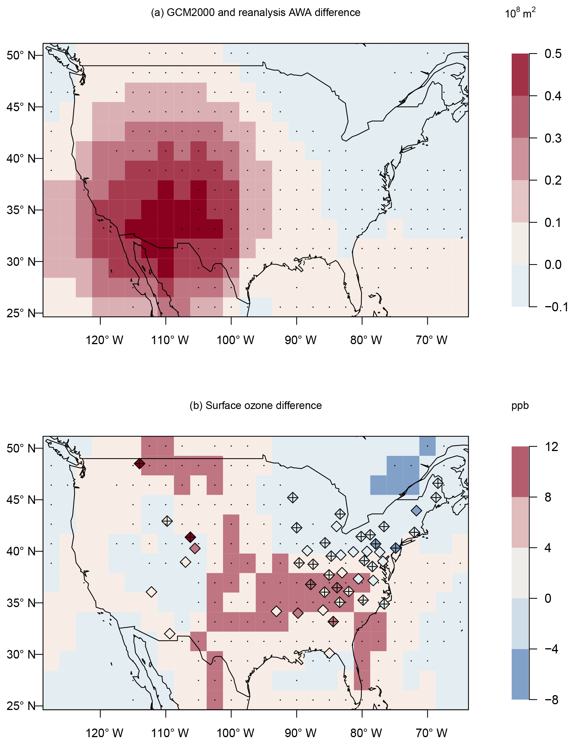
Figure 6 (a) JJA difference in AWA between the GCM2000 simulation (2006–2025) and the ERA-Interim reanalysis (1995–2014) (10⁸ m²). (b) Change in MDA8 ozone from the linear regression model derived from the GCM2000 simulation (shaded) or the measurements (diamonds) using the AWA difference (calculated from GCM2000 simulation and ERA-Interim reanalysis) projection as the explanatory variable. Plus signs and stippling represent where the ozone difference is significant (at the 5 % significance level) at CASTNET sites and model grids, respectively.

Ozone in the northeastern US is particularly sensitive to AWA over the East Coast (see Sect. 3.3.2). The ozone decrease over the northeast US in Fig. 6 can be attributed to decreased anticyclonic activity over the East Coast in the GCM2000 simulation, which acts to decrease the advection of pollutant into the northeast. From the mid-Atlantic states to the southeastern states, ozone is particularly sensitive to AWA to the west and southwest of a particular site (Sect. 3.3.2). Ozone differences in these regions are impacted by the stronger ridging in the southwest US in the GCM2000 simulation relative to the ERA-Interim reanalysis. The positive ozone anomaly in the southeastern US in Fig. 6 can thus be attributed to the relatively large anticyclonic activity in the GCM2000 simulation in the southwestern US, which acts to advect continental air with relatively high pollutants concentrations into the southeastern US.

3.3.2 Future AWA changes: ozone impacts

Future changes in JJA 500 hPa geopotential height and wave activity between the GCM2100 simulation and the GCM2000 simulation are given in Fig. 7. Significant increases in geopotential height occur everywhere, with increases of approximately 30–60 m over most of the US. These increases can be attributed to mid-to-high latitude warming in the future climate. The geopotential height increase tends to be larger at higher latitudes consistent with other model projections (e.g., Yue et al., 2015; Vavrus et al., 2017). By definition the zonally symmetric change in geopotential height has no equivalent change in AWA, but regional changes in AWA reflect future changes in the waviness of the flow. The most pronounced future change is the large anticyclonic wave activity enhancement over the southwestern US (Fig. 7b), also seen in the total wave activity (Fig. 7d), in response to increased ridging in this region. Using a different metric to characterize the waviness of the circulation, Vavrus et al. (2017) found a large increase in the waviness of the flow (measured as sinuosity) over the US centered at 42^∘ N. In contrast the CWA shows relatively small changes in the future (Fig. 7c).

Figure 7 JJA-simulated difference between the GCM2100 and the GCM2000 for 500 hPa geopotential height (m) (a), anticyclonic wave activity (10⁸ m²) (b), cyclonic wave activity (10⁸ m²) (c), and total wave activity (10⁸ m²) (d) between 24 and 53^∘ N. Note that in the Northern Hemisphere the cyclonic wave activity and total wave activity are negative. Here the change in magnitude is presented. Stippling represents where the change is significant at the 5 % level using a Student t test.

All future ensembles examined show a similar pattern in the future change in AWA (Fig. 8) with large increases in AWA in the western and southwestern US. Here we examine both the AWA change in the climate-change-only simulations (GCM2100 minus GCM2000), where forcing from short-lived constituents and methane remains constant over the twenty-first century, and we examine the AWA change from each of the three ensemble members of the REFC2 simulation, where the forcing from the short-lived constituents and methane follows the RCP6 scenario. Note that these future changes in AWA are similar to present-day differences between the GCM2000 simulation and the ERA-Interim reanalysis (Fig. 6). Despite the similar pattern in future AWA change in all simulations, there are also some significant differences in the strength, position and, orientation of the AWA anomaly in the western US among simulations. These variations are evident even in a 10-year average variability and can be attributed to the substantial internal variability of long-term tropospheric flow (e.g., Deser et al., 2012). As we show below, these differences result in substantial uncertainty as to the future ozone change due to changes in regional circulation.

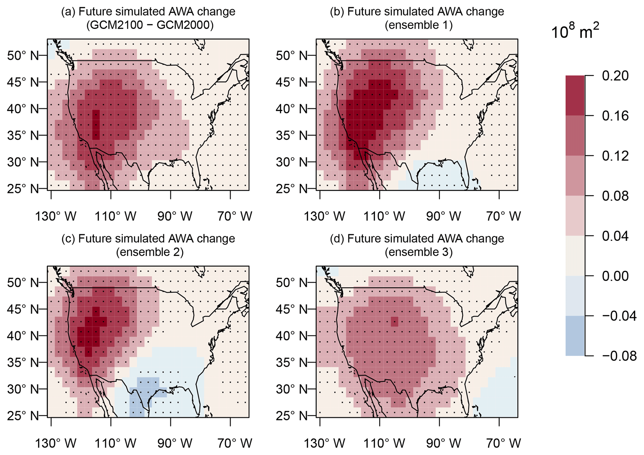
Figure 8 JJA difference in AWA (10⁸ m²) between the GCM2100 and the GCM2000 simulation (a) and from the three ensemble members of the REFC2 simulation between 2090 and 2099 and 2000 and 2009 (b–d). Stippling represents where the change is significant at the 5 % level using a Student t test.

To predict the future change in ozone due to AWA changes we use the regression between ozone and AWA determined in the present climate. To check that this relationship does not change in the future we calculate the slopes of the linear regression model using AWA and ozone from the present climate (GCM2000) and the future climate (GCM2100), and then we construct the 95 % confidence intervals for the two slopes. For all the grid points, the 95 % confidence intervals of the two slopes overlap. Therefore, we assume the regression between AWA and ozone does not substantially change in the future.

Regional ozone changes attributed to the future changes in AWA range from approximately −2.5 to 2.5 ppb (Fig. 9). The predicted future changes are smaller than those derived from present-day differences between the GCM2000 simulation and the measurement-derived ERA-Interim reanalysis (Fig. 6) but show an overall similar pattern. All future simulations show an increase in ozone over a portion of the southeastern US, although the amplitude and extent of the increase vary from simulation to simulation. The ozone change over the northeast US is inconsistent among the different simulations with slight ozone increases or decreases simulated. Over the Rocky Mountains ozone decreases are predicted when future changes are calculated with the simulated regression coefficients, but ozone increases are predicted when calculated with measurement-derived coefficients. The variation in ozone change among the different ensembles is consistent with the unforced, low-frequency climate-induced variability in ozone as analyzed in Barnes et al. (2016).

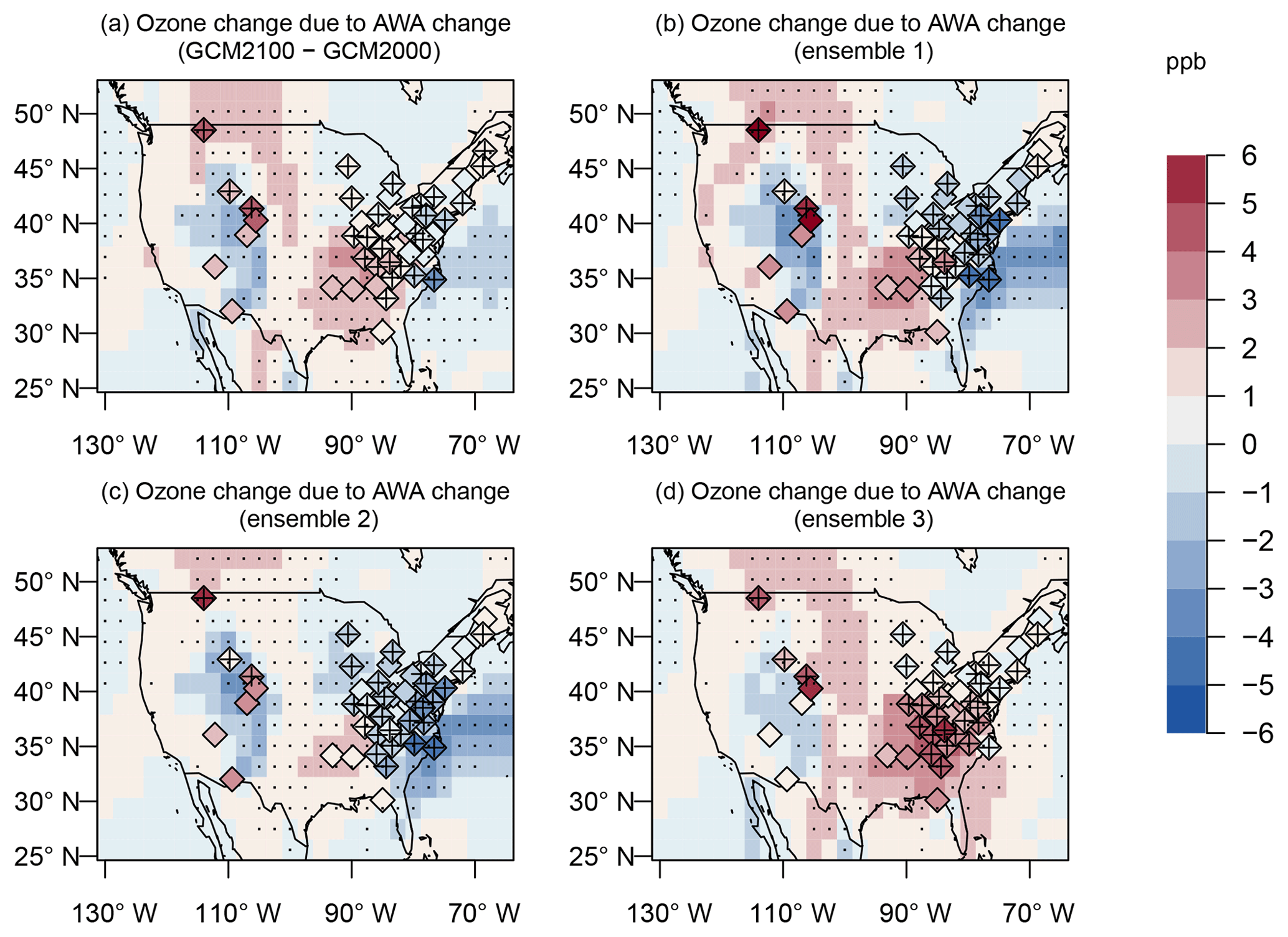
Figure 9 Change in MDA8 ozone from the linear regression model derived from the GCM2000 simulation (shaded) or the measurements (diamonds) using the AWA difference projection as the explanatory variable. Differences in AWA are calculated between the GCM2100 simulation and GCM2000 simulation (a) from the three ensemble members of the REFC2 simulation between 2090 and 2099 and 2000 and 2009 (b–d). Plus signs and stippling represent where the future change of AWA is significant (at the 5 % significance level) at CASTNET sites and model grids, respectively.

Comparing the GCM2100 and the GCM2000 simulations (Fig. 10), future changes in ozone over land range from approximately −1 to 5 ppb. It is clear that overall, changes in circulation, as defined through changes in AWA, cannot explain future ozone changes. However, in many locations the change in ozone predicted from the change in wave activity between the GCM2100 and GCM2000 simulations is consistent with the actual GCM-simulated ozone change. The ozone increase in the southeastern US through the Pacific Northwest and the ozone decrease in the interior southwest predicted by the linear regression model (in particular the regression based on the GCM2000 simulation) (see Fig. 9) largely agrees in sign with the ozone difference between the GCM2100 simulation and the GCM2000 simulation (Fig. 10). In many of these locations the linear regression prediction is consistent with the magnitude of the simulated ozone change. Overall, the RMSE of the linear regression model ozone change compared with the GCM-simulated ozone change is ∼2 ppb. In the northeastern US, the predicted ozone change from the AWA analysis is negative, the opposite of the GCM-simulated difference. It is likely that in this region of high-ozone precursor emissions chemical considerations dictate the ozone change and that changes in circulation play a minor role.

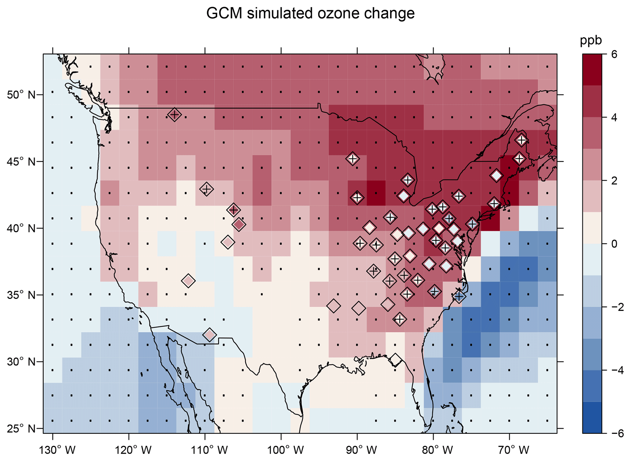
Figure 10 JJA change in MDA8 ozone between the GCM2100 simulation and the GCM2000 simulation (ppb, shaded). Diamonds give the change in MDA8 ozone in the linear regression model derived from the measurements using the AWA difference (between GCM2100 and GCM2000) projection as the explanatory variable.

Applying the linear regression model based on geopotential height to a future climate gives a completely different picture from the one based on AWA (Fig. S3b). The model based on geopotential height predicts much larger future ozone changes, up to 10 ppb, over the southeastern US and ozone increases over southeastern Canada of up to 5 ppb. In the present climate, the linear regression model based on geopotential height is at least as good as that based on AWA. The difference in future projections can be explained by the fact that changes in AWA represent changes in the waviness of the circulation, but they do not reflect changes in the mean circulation. In contrast, the metric based on the geopotential height includes changes in the zonal mean and thus reflects the change caused by warming in general, including a general northward movement in the zonally averaged jet stream.

The sensitivity to changes in the AWA pattern (ppb m⁻²) in the GCM2000 simulation and the sensitivity multiplied by the future change in AWA (GCM2100 minus GCM2000) is given in Fig. 11. Note that the overall predicted ozone change is proportional to the sum of the latter metric over the study region (Fig. 11b, d, f). The CASTNET site HOW132 in the northeast US is positively sensitive to AWA changes over the East Coast, but negatively sensitive to changes further inland over the Midwest, particularly in the upper Midwest. As a result of these competing influences the overall future change due to regional circulation changes is small (Fig. 11b). The effects of future AWA increases over both the East Coast and over the Midwest largely cancel each other out. The sensitivity to changes in AWA in the mid-Atlantic region (e.g., at station PAR107) and in the southeast (e.g., at station GAS153) are opposite to the above. For these sites, increases in the AWA in the central US increase the ozone anomaly (i.e., the sensitivity is positive), while AWA increases off the East Coast act to decrease the ozone anomaly (i.e., the sensitivity is negative). At these sites the large positive change in AWA over the Midwest tends to dominate the future signal as the increased anticyclonic circulation over the Midwest results in more offshore flow.

Figure 11 Regression coefficients between MDA8 ozone during JJA at representative sites (star sign) and AWA in the study region (a, c, e). Regression coefficients multiplied by the change in AWA between the GCM2100 simulation and the GCM2000 simulation (b, d, f). The predicted change in ozone from the linear regression model is proportional to the sum of all points (in b, d, f) over the domain (Eq. 6). Stippling represents where the regression coefficient is significant at the 5 % significance level.

4 Discussion and conclusions

We use wave activity in a univariate linear regression model to quantitatively relate interannual variations in the large-scale flow over the US to interannual variations in ozone. At any point, the impact of AWA on ozone is measured through a projection of AWA onto the spatial structure of the sensitivity of ozone to AWA. Throughout much of the US variations in wave activity explain 30 %–40 % of the simulated and measured ozone variance (Fig. 5). While the explanatory value of AWA is not exceptionally high, in general the correlation between individual meteorological variables and ozone is not high (e.g., Sun et al., 2017; Kerr and Waugh, 2018). The interannual correlation between ozone and temperature is somewhat stronger than the relationship between AWA and ozone over the study region (mean of the former is 0.48 and mean of the latter is 0.24). Nevertheless, as a metric of changes in the regional circulation, AWA explains a significant fraction of interannual ozone change. Changes in AWA, of course, impact local variables that directly control ozone (e.g., temperature and boundary layer venting).

The variance explained by using geopotential height as the explanatory variable instead of AWA (Fig. S3a) in the linear regression is roughly equivalent or somewhat more than that using wave activity. The advantage of using wave activity is its theoretical relationship to the large-scale wave dynamics of the atmospheric circulation and its utility as a metric for blocking (Martineau et al., 2017). In addition, AWA is not explicitly sensitive to changes in zonal mean circulation characteristics, for example a general northward movement of the jet stream or a uniform increase in temperature (or equivalently geopotential thickness). Thus future changes in AWA give a fundamentally different picture of future ozone changes from changes in the geopotential height (Fig. 9 versus Fig. S3b). In particular, changes in AWA are related to changes in the local waviness of the flow.

As determined through the regression coefficients, there are two main centers of sensitivity for ozone variability over the eastern US: one in the Midwest and one along the East Coast (Fig. 11). The center along the East Coast is likely controlled by the strength and position of the Atlantic anticyclone; the center over the Midwest is controlled by the strength and position of the AWA center over the western US. These centers control the flow of air from Gulf of Mexico into the eastern US and the transport of high-ozone air under anticyclonic conditions into the northeastern US. In most of the simulations analyzed here increased future AWA tends to increase ozone in the interior southeast and decrease it over the northeastern states.

The regression coefficients determining the ozone sensitivity to AWA within the study region are remarkably similar in the model simulations and in the measurement-derived analysis, at least for the three representative points examined (Fig. S2). Additionally, the ozone change due to changes in AWA in the model and measurements has usually the same sign everywhere with the same approximate magnitude (Fig. 9) suggesting that the agreement in the model-derived and measurement-derived sensitivities is widespread. The exception to this agreement occurs at some of the CASTNET sites in the interior western US, where the measurements and model predict a future ozone change of opposite sign. It is possible that local topographical features in this part of the US, not captured by the model, are important. The similarity between modeled and measured sensitivities suggests that at most grid points the simulations do capture the conditions under which high (or low) ozone occurs. Thus it is likely that model-measurement discrepancies in the ozone change due to changes in AWA are due to differences in the AWA and not in the relation between AWA and ozone at a point.

Deficiencies in the simulation of the Atlantic anticyclone have been related to deficiencies in the simulation of ozone variability in the northeastern US. In the measurement-derived analysis, the ozone variability associated with the MCA is large in the northeastern US; in the measurements the relation between AWA and ozone is strong, and changes in AWA can explain a significant fraction of the ozone variability (Fig. 5). In contrast, in the simulated MCA the relationship between ozone variability and AWA is weak in the northeastern US. Consistent with this, the changes in AWA are not significantly related to changes in ozone in the northeastern US (Fig. 5). We attribute these differences between the simulation and the measurements to differences in the simulation of the Atlantic anticyclone.

This has implications for future ozone extremes over the northeastern US. A rather robust feature of future climate change is the westward movement of the Atlantic anticyclone from its current position (Shaw and Voigt, 2015). In the GCM2000 simulation the Atlantic anticyclone is already situated considerably west of its climatological position. If the Atlantic anticyclone indeed moves westward in the future, the MCA analysis of the GCM2000 simulation (Fig. 3d) (with its westward shift of the Atlantic anticyclone) might be a good representation of future ozone variability. If so we might expect that future high-ozone pollution episodes associated with the Atlantic anticyclone over the northeastern US will shift westward with a consequent decrease in the variability of ozone over the northeast US.

The future simulations show considerable variability in their change in wave activity compared to present day. This longer-timescale variability has been pointed out with regards to climate (e.g., Deser et al., 2012) and with regards to changes in ozone (Hess and Zbinden, 2013; Lin et al., 2014; Hess et al., 2015; Barnes et al., 2016). Even on these fairly long timescales the future change in ozone due to circulation variability is on the order of 2 ppb. Nevertheless, while some of the details differ, all future simulations examined with the CESM show a large enhancement in anticyclonic wave activity and geopotential height in the southwestern US. This enhancement of wave activity drives a significant fraction of the predicted future ozone change due to changes in wave activity. In all simulations this causes ozone increases through parts of the southeast US (Fig. 9). In the northeastern US future ozone change due to changes in AWA is generally small, ranging from about +1 to −1 ppb depending on the simulation (Fig. 9). Changes in AWA explain aspects of the future ozone change (GCM2100 minus GCM2000) outside the northeast US.

The difference in AWA between the GCM2000 simulation and the ERA-Interim reanalysis is large (Fig. 6). The present-day differences in AWA might be due to meteorological variability, or perhaps more likely due to model bias. This implies that in many locations ozone changes due to model bias (or variability) in AWA lead to ozone changes larger than those projected by future changes, with ozone increases of approximately 4–8 ppb in the southeastern US. The difference in AWA between the GCM2100 simulation and the GCM2000 simulation is similar to that between the GCM2000 simulation and the ERA-Interim reanalysis. Thus in many ways compared to the ERA-Interim reanalysis the GCM2000 simulation looks like what one would expect in a future climate. Over the western US the AWA anomaly gets larger as one goes from the ERA-Interim reanalysis to the GCM2000 simulation to the GCM2100 simulation. Similarly, off the East Coast of the US the Atlantic anticyclone moves northwestward as one goes from the ERA-Interim reanalysis to the GCM2000 simulation to the GCM2100 simulation (Fig. 4).

The GCM2000 simulation is similar to the future simulations in the westward placement of the Atlantic anticyclone and the strength of the anticyclone over the western US. Given the fact that AWA in the GCM2000 simulation is in many ways more similar to that of the GCM2100 simulation than the ERA-Interim reanalysis, one might question whether the difference between the GCM2100 and GCM2000 simulations provides an accurate metric for future change. The difference between the GCM2100 and GCM2000 simulations is also consistent with the difference between the twenty-first century REFC2 ensemble members. The GCM2100 minus GCM2000 difference does not stand out compared to the REFC2 ensemble members (Fig. 8). Thus the difference in AWA between the GCM2000 simulation and the ERA-Interim reanalysis (Fig. 6), or between the GCM2100 simulation and the ERA-Interim reanalysis (Fig. S4), might be a better estimator of what to expect in the future. If the latter is the case, increases in ozone of up to 15 ppb or decreases of up to 8 ppb might be expected due to changes in future AWA (Fig. S4).

In conclusion, we show that wave activity, as a metric of large-scale mid-latitude flow, provides a powerful tool to relate the larger-scale tropospheric circulation to local surface ozone. In particular, we use changes in wave activity to better understand the impact of model biases and future circulation changes on simulated surface ozone concentrations. A similar methodology could be expanded to other climate variables (e.g., temperature) or applied as a means of relating the larger-scale flow field to surface ozone or temperature extremes. In all future simulations we find regionally robust summertime changes in wave activity over the western and southwestern US. It would be interesting to see if these future changes are robust across different models and to further quantify their impact on predicted summertime climate change.