the Creative Commons Attribution 4.0 License.
the Creative Commons Attribution 4.0 License.
 | 08 Oct 2019
Common volume satellite studies of polar mesospheric clouds with Odin/OSIRIS tomography and AIM/CIPS nadir imaging
Susanne Benze
Jörg Gumbel
Ole Martin Christensen
Cora E. Randall
Two important approaches for satellite studies of polar mesospheric clouds (PMCs) are nadir measurements adapting phase function analysis and limb measurements adapting spectroscopic analysis. Combining both approaches enables new studies of cloud structures and microphysical processes but is complicated by differences in scattering conditions, observation geometry and sensitivity. In this study, we compare common volume PMC observations from the nadir-viewing Cloud Imaging and Particle Size (CIPS) instrument on the Aeronomy of Ice in the Mesosphere (AIM) satellite and a special set of tomographic limb observations from the Optical Spectrograph and InfraRed Imager System (OSIRIS) on the Odin satellite performed over 18 d for the years 2010 and 2011 and the latitude range 78 to 80∘ N. While CIPS provides preeminent horizontal resolution, the OSIRIS tomographic analysis provides combined horizontal and vertical PMC information. This first direct comparison is an important step towards co-analysing CIPS and OSIRIS data, aiming at unprecedented insights into horizontal and vertical cloud processes. Important scientific questions on how the PMC life cycle is affected by changes in humidity and temperature due to atmospheric gravity waves, planetary waves and tides can be addressed by combining PMC observations in multiple dimensions. Two- and three-dimensional cloud structures simultaneously observed by CIPS and tomographic OSIRIS provide a useful tool for studies of cloud growth and sublimation. Moreover, the combined CIPS/tomographic OSIRIS dataset can be used for studies of even more fundamental character, such as the question of the assumption of the PMC particle size distribution.
We perform the first thorough error characterization of OSIRIS tomographic cloud brightness and cloud ice water content (IWC). We establish a consistent method for comparing cloud properties from limb tomography and nadir observations, accounting for differences in scattering conditions, resolution and sensitivity. Based on an extensive common volume and a temporal coincidence criterion of only 5 min, our method enables a detailed comparison of PMC regions of varying brightness and IWC. However, since the dataset is limited to 18 d of observations this study does not include a comparison of cloud frequency. The cloud properties of the OSIRIS tomographic dataset are vertically resolved, while the cloud properties of the CIPS dataset is vertically integrated. To make these different quantities comparable, the OSIRIS tomographic cloud properties cloud scattering coefficient and ice mass density (IMD) have been integrated over the vertical extent of the cloud to form cloud albedo and IWC of the same quantity as CIPS cloud products. We find that the OSIRIS albedo (obtained from the vertical integration of the primary OSIRIS tomography product, cloud scattering coefficient) shows very good agreement with the primary CIPS product, cloud albedo, with a correlation coefficient of 0.96. However, OSIRIS systematically reports brighter clouds than CIPS and the bias between the instruments (OSIRIS – CIPS) is sr−1 ( sr−1) on average. The OSIRIS tomography IWC (obtained from the vertical integration of IMD) agrees well with the CIPS IWC, with a correlation coefficient of 0.91. However, the IWC reported by OSIRIS is lower than CIPS, and we quantify the bias to −22 g km−2 (±14 g km−2) on average.
- Article
(4943 KB) - Full-text XML
- BibTeX
- EndNote


Polar mesospheric clouds (PMCs) are the highest and coldest clouds of the Earth's atmosphere. During daylight conditions, PMCs are too faint to be observed by the naked eye, but during twilight, when the lower atmosphere lies in Earth's shadow, PMCs become visible against the dark sky when they efficiently scatter light from the sun under the horizon. The striking appearance of a silvery shining veil against the darker summer night sky has also given them the name noctilucent clouds (NLCs). Despite the remarkably dry environment of the summer polar mesosphere of only a few parts per million of water, PMCs can form because the wave-driven residual meridional inter-hemispheric circulation (Lindzen, 1981; Garcia et al., 1985) causes upwelling of air from the stratosphere, and the rising motion over the summer pole leads to strong adiabatic cooling of the summer polar mesospheric region (Fritts and Alexander, 2003). Resulting mesopause temperatures of typically 130–150 K (Lübken, 1999) make it possible for water vapour to condense on cloud nuclei, forming visible PMCs. During the last two decades, extensive research has contributed to knowledge about PMC formation and composition. It is now well established that the clouds consist of water ice that has nucleated onto meteoric smoke material (Hervig et al., 2001, 2009), and that nucleation occurs in bursts at the mesopause (Megner, 2011; Kiliani et al., 2013). The ice particles grow in size by condensation of the surrounding water vapour and sediment when they grow large enough and typically become visible when they reach sizes above 20–30 nm (Rapp et al., 2002; Rapp and Thomas, 2006). Eventually, they descend into a sub-saturated air mass and sublimate.
Ever since the first observations of these night-shining clouds over 130 years ago (Backhouse, 1895; Jesse, 1885; Leslie, 1985 ), the clouds have been studied extensively and continue to be a major subject of middle atmospheric research. This is related to the fact that PMCs are very sensitive to changes in temperature and water vapour and therefore serve both as tracers for long-term changes of the middle atmosphere where direct observations are limited (DeLand et al., 2006; DeLand and Thomas, 2015) and tracers for the dynamics of the polar summer mesosphere (e.g. Fritts et al., 1993). PMCs are frequently used as a tool to study wave activity in the mesosphere (Witt, 1962). Gravity waves excited at lower altitudes that propagate through the PMC layer alter the cloud microphysics and leave behind a detectable footprint, which manifests as a variation in cloud brightness or cloud height that can be observed both using ground-based instruments and satellites. Propagating gravity waves create a downward and upward motion of the PMC layer, and the adiabatic heating and cooling associated with regions of downward and upward motion will cause sublimation and growth of the cloud ice. The resulting structures in the cloud layer can be used to detect and quantify gravity waves that are present in the mesopause region (Thurairajah et al., 2017; Hart et al., 2018). Gravity wave signatures from PMC albedo variations observed by the nadir Cloud Imaging and Particle Size (CIPS) experiment on the Aeronomy of Ice in the Mesosphere (AIM) satellite (Russel et al., 2009) have for example been used to investigate both small-scale gravity waves (Chandran et al., 2009; Taylor et al., 2011) and large-scale gravity waves (Chandran et al., 2010; Zhao et al., 2015). Additionally, CIPS has proven an excellent tool to study various types of cloud structures, such as voids, bands, ice rings and fronts, that are connected to the complex small-scale dynamics present in the summer mesopause region (Thurairajah et al., 2013).
Extensive research has led to an increased knowledge on the climatology of PMCs. A number of recent studies suggest that PMC occurrence frequency has increased in recent decades (e.g. Hervig et al., 2016; Lübken et al., 2018; and references therein).
DeLand and Thomas (2015) show an increase in PMC ice water content (IWC) at latitudes between 50 and 82∘ both in the Northern Hemisphere and the Southern Hemisphere. Fiedler et al. (2016) report on similar PMC trends from lidar observations at 69∘ N. In their study, they analyse a 22-year PMC dataset and confirm that PMCs are becoming brighter and occur more often. Suggestions that observed changes in PMC properties over time are connected to the increase in methane and carbon dioxide in the troposphere (Thomas et al., 1989; Thomas and Oliviero, 2001) are still under debate. Recently, Lübken et al. (2018) presented model studies of the anthropogenic effect on PMCs at mid-latitudes by simulating the increased amounts of carbon dioxide and water vapour in the mesosphere since the beginning of industrialization. Their study suggests that increased amounts of water vapour (due to increased methane) is the main reason for the increasing visibility of PMCs at mid-latitudes in the modern era, and that a cooling of the mesosphere is only of secondary importance.
The geographical extent and variation of the PMC layer are monitored continuously by both ground-based instruments and satellites, which each possess their advantages and disadvantages. For example, NLC camera networks and ground-based lidars possess the advantage of being able to observe the clouds with very high temporal resolution. NLC camera networks can capture the horizontal evolution of a geographically limited region of the PMC layer. Numerous ground-based studies from NLC camera networks have led to remarkable insight into the complexity of spatial structures of the clouds, planetary wave influence on NLC occurrence frequency, gravity wave effects on the NLC layer and cloud height measurement (e.g. Dalin et al., 2016, 2015; Kirkwood and Stebel, 2003; Witt, 1962). Ground-based lidar systems on the other hand possess the unique capacity to monitor the vertical structure of the cloud with resolutions as fine as 30 s and 50 m (Baumgarten et al., 2012) and give detailed insight into the microphysical processes of a cloud as well as climatology and long-term changes of PMCs (Baumgarten et al., 2012; Fiedler et al., 2016; Kaifler et al., 2013; Ridder et al., 2017; Shibuya et al., 2017; Suzuki et al., 2013). Ground-based instruments alone, however, lack the ability to monitor the longitudinal and latitudinal variations. Polar-orbiting satellites, on the other hand, are able to provide information about the climatology and global distribution of PMCs (e.g. Bailey et al., 2015; Hervig et al., 2016, Liu et al., 2016) as well as detailed information about horizontal variations of cloud parameters and wave effects on cloud microphysics (e.g. Rusch et al., 2016; Hart et al., 2018). Each satellite geometry has its limitations: nadir-pointing instruments observe horizontal cloud structures but can provide no or limited information about vertical structures (Hart et al., 2018). Limb-scanning instruments provide information on vertical cloud structures but have only coarse horizontal resolution with gaps between observations. Due to instrument design, limb-viewing instruments observe PMC as a function of tangent altitude, not the real altitude. As a consequence, the PMC retrieval cannot separate low-lying clouds from clouds in the foreground or in the background. The PMC retrieval for the limb-viewing Optical Spectrograph and Infrared Imager System (OSIRIS) (Llewellyn et al., 2004) on the Odin satellite (Murtagh et al., 2002) assumes that the PMC layer is spatially homogeneous along the instrument line of sight (LOS) for the normal limb scans. This assumption is clearly a simplification, and numerous observations from nadir-viewing satellites, lidar and ground-based cameras (e.g. Baumgarten et al., 2012; Dalin et al., 2016; Thurairajah et al., 2013; Witt, 1962) have shown that the PMC cloud layer is highly structured both in horizontal and vertical extent.
To overcome the limitation from the assumption of a spatially homogeneous cloud layer and to enable the retrieval of clouds as a function of actual height instead of tangent height, the application of a two-dimensional tomographic retrieval for OSIRIS has been presented by Hultgren et al. (2013). The tomographic approach for OSIRIS retrievals (described in Sect. 2) provides a tool to study both vertical and horizontal variations of cloud microphysical properties on a local scale, which is useful for detailed studies of cloud growth and destruction (Christensen et al., 2016; Megner et al., 2016). An early attempt to apply a direct (tomographic) retrieval for a limb-viewing instrument was investigated almost two decades ago. The first approach was carried out by Livesey and Read (2000), who developed a tomographic 2-D retrieval for the Microwave Limb Sounder (MLS) instrument on the Aura satellite. A tomographic reconstruction of atmospheric constituents and gases can be performed using multiple exposures from multiple viewing angles. The tomographic technique has previously been used to study middle atmospheric phenomena other than PMCs, for example gravity wave activity in airglow in the mesopause region (e.g. Nygren et al., 2000; Song et al., 2017), and stratospheric mesoscale gravity waves (Krisch et al., 2017; 2018). More recently, Hart et al. (2018) successfully demonstrated the first application of a tomographic technique to CIPS on AIM. They were able to project a novel 2-D PMC surface map with gravity wave signatures, providing valuable information on wave characteristics such as wave amplitude and dominant horizontal wavelengths. For the OSIRIS instrument, Degenstein et al. (2003, 2004) first showed the possibility to retrieve both vertical and horizontal structures from a series of limb images taken from the OSIRIS infrared imager and were able to map volume emission rates of the oxygen infrared atmospheric band.
In this paper, we perform a detailed common volume (CV) study of PMC cloud brightness and ice mass density (IMD) from the Odin OSIRIS tomographic retrievals and coincident PMC observations from CIPS on AIM. The occasions for Odin's special tomographic scans were chosen to coincide both in time and space with the CIPS instrument. A comparison of the two instruments is therefore ideally suited for instrument validation and the combination of the two datasets will be valuable in future studies of cloud–wave interaction, studies on particle sizes and studies on how the retrieved cloud properties are affected by cloud inhomogeneities. Many scientific questions about the PMC life cycle are connected to the two- or three-dimensional structure of the clouds. Important questions concern, for example, the effect of gravity waves or dynamical instabilities on the growth, sublimation or appearance of the clouds. Combined observations by (horizontally resolved) nadir instruments and (vertically resolved) limb instruments have large potential to address such multi-dimensional questions. This is true in particular if the datasets involve tomographic analysis, as in the case of the OSIRIS data utilized here.
Taking into account that the satellites have different viewing geometry, resolution and sensitivity, we analyse cloud brightness and the cloud ice in the CV and perform a detailed error analysis. One advantage of comparing tomographic OSIRIS observations to CIPS observations is that both instruments measure scattered radiance, although OSIRIS measures with limb-viewing geometry and CIPS uses nadir-viewing geometry. Another advantage is that the same assumption regarding the mathematical shape of the particle size distribution, namely a Gaussian distribution, is used in both the OSIRIS and the operational CIPS v4.2 retrieval.
The specific aims of this satellite comparison study are as follows:
- 1.
Perform the first thorough error characterization of the Odin OSIRIS tomographic dataset.
- 2.
Validate the tomographic retrieval and error characterization by comparing PMC albedo and IWC from the Odin/OSIRIS retrievals and AIM/CIPS retrievals.
- 3.
Establish a consistent method for comparing cloud properties from a limb sounding tomographic dataset to a nadir-viewing instrument.
- 4.
Produce a combined dataset of Albedo and IWC that will facilitate future studies of the PMC life cycle and PMC particle sizes.
This study focuses on comparing the albedo and IWC between the instruments. A future goal is to produce a combined dataset that can be used to study for example more fundamental issues such as the assumptions of PMC the size distribution of PMCs, an assumption that has been questioned in the past. Each instrument used alone can only provide either very fine horizontal resolution (CIPS) or vertical/coarse horizontal resolution (tomographic OSIRIS). However, when combined in an efficient way, OSIRIS can provide vertical information on cloud structures such as double cloud layers or voids, ice distribution at different altitude levels, and information about the existence of particles of different sizes on different altitude levels that can complement the high horizontal resolution of the clouds from CIPS. Additionally, the combined dataset can be used to investigate how waves (inferred from albedo variations in CIPS) affect the cloud lifetime and how nucleation–sublimation processes affect the vertical distribution of cloud properties (inferred from a vertical cross section from OSIRIS).
The paper is structured as follows. First, in Sect. 2, the OSIRIS tomographic technique is introduced together with a thorough error characterization of the OSIRIS tomography PMC scatter coefficient and IMD. Additionally, this section describes the CIPS PMC dataset and known uncertainties of cloud albedo and IWC. In Sect. 3, the method used for the instrument comparison is described, including a discussion of the challenges in making tomographic limb and nadir observations consistent. In Sect. 4, the results of the comparison are presented and discussed. Section 5 provides the conclusions.
2.1 Odin OSIRIS
The Swedish-led Odin satellite (Murtagh et al., 2002) was launched on 20 February 2001, into an almost Sun-synchronous polar orbit at 600 km with ascending node near 18:00 local solar time. The Odin mission began as a joint project between aeronomy and astronomy, with the primary focus of the aeronomic part of the mission on coupling processes in the atmosphere, better understanding of ozone variation and processes in the middle atmosphere, and processes that govern PMC formation and mesospheric variability. Odin carries two instruments, the Sub-Millimeter Radiometer (SMR) (Urban et al., 2007) and OSIRIS (Llewellyn et al., 2004). OSIRIS consists of an atmospheric limb-scanning spectrometer and an infrared imager with the ability to measure vertical profiles of atmospheric trace gases and ice layers in the middle atmosphere (Karlsson and Gumbel, 2005). The Odin instruments scan the limb of the atmosphere in the forward direction as the satellite nods up and down while moving in its polar orbit. The OSIRIS spectrometer observes scattered sunlight as limb radiance in the wavelength range from 275 to 810 nm with a spectral resolution of about 1 nm. Odin can be operated in different modes that regulate the vertical resolution and altitude region depending on the species of interest. In a standard stratospheric–mesospheric mode, the satellite typically scans the atmosphere from 7 to 107 km. In 2010, a so-called tomographic mode was developed, scanning only PMC altitudes between typically 70 and 90 km. Since 2010, Odin has continued to perform regular observations in this tomographic mode for selected orbits both in the Northern Hemisphere and in the Southern Hemisphere up until the present. In the tomographic mode, the distance between subsequent scans is shorter, which increases the horizontal sampling compared to the normal mode. The extended number of lines of sight through a cloud volume produces sufficient information to tomographically retrieve two-dimensional distributions of the cloud scattering coefficient as a function of height and horizontal distance. The tomographic algorithm inverts the observed limb radiance into an estimate of the retrieved local scattering coefficient, a measure of the cloud brightness. The tomographic retrieval is based on the multiplicative algebraic reconstruction technique (MART) developed by Lloyd and Llewellyn (1989) and further developed and adapted to OSIRIS data by Degenstein (1999) and Degenstein et al. (2003, 2004). It was described in detail by Hultgren et al. (2013) and Hultgren and Gumbel (2014). MART is based on maximum probability theory that solves the problem on a ray-by-ray basis until the retrieval converges.
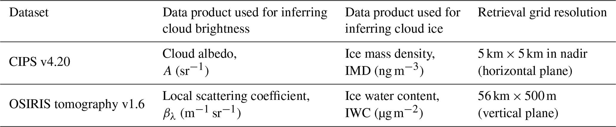
The limb radiance is measured by Odin as a function of tangent altitude, while the tomography retrieves the local scattering coefficient as a function of actual altitude and angle along orbit (AAO). AAO runs from 0 to 360∘ and simply denotes the position of the tangent point along the satellite orbit, starting from 0∘ when the satellite is crossing the Equator, increasing to 90∘ at the northernmost position, etc. One important advantage of the tomographic retrieval is that cloud brightness can be expressed as a local feature. This solves the problem of ordinary limb retrievals that clouds in the fore- and background cannot be distinguished from low-altitude clouds (Karlsson and Gumbel, 2005). The OSIRIS across-track field of view (FOV) through the PMC layer is not constant since it depends on the satellite altitude and the distance from the satellite to the limb, which varies with tangent altitude. The viewing angle of OSIRIS is 35.8 arcmin across the track, which yields a value close to 30 km for the FOV width at the tangent altitude in the PMC region for 2010 and 2011, and this is the value that will be used in this study. Over the length of one common volume element (the reader is referred to Fig. 3 for a schematic of the common volume element), the across-track width of the FOV changes by 2 %, or 600 m. This is largely negligible in comparison with the spatial extent of one CIPS pixel and therefore not taken into account in this study.
The tomographic retrieval uses a grid of m (AAO × altitude), which corresponds to 56 km×500 m in the horizontal and vertical direction. In the following we refer to this OSIRIS tomographic retrieval grid as the OSIRIS “pixel” to be consistent with the terminology used for CIPS. The actual horizontal resolution of the retrieval is coarser than this grid and is defined by the retrieval's averaging kernel. To retrieve cloud information at a given point, the tomographic algorithm combines information from a large number of nearby lines of sight, each covering several hundred kilometres of path through the PMC layer. In order to characterize the ability of the algorithm to resolve cloud structures, measurement simulations have been performed on a cloud filling a single OSIRIS pixel. These result in averaging kernels that are typically described by a Gaussian shape with a full width at half maximum (FWHM) of 280 km. In the case of the OSIRIS tomography, the resolution is limited by the relatively sparse distribution of measurements. Limb radiances from individual lines of sight are recorded once per second, while the satellite scans the tangent altitudes with a speed of about 0.75 km s−1, and moves along its orbit at about 7 km s−1. As a result, the ability to resolve a given cloud structure varies stochastically depending on how the nearest lines of sight happen to be distributed relative to the cloud structure. Applying an averaging kernel of 280 km to the data will thus account for lowest possible resolution, although if a cloud structure is in a more favourable position to the closest lines of sights, the ability to resolve this structure increases. To account for this, horizontal resolutions of both 280 km (typical averaging kernel) and 56 km (length of OSIRIS retrieval pixel) will be considered as limiting cases when comparing individual OSIRIS and CIPS measurements in Sect. 4.2.
The measured PMC limb radiance contains contributions from molecular Rayleigh scattering from the background atmosphere as well as instrumental effects, e.g. baffle scattering and offset due to dark current. Therefore, a separation of the pure cloud signal from the background is needed before the tomographic retrieval can be performed. As the short limb scans in tomographic mode do not cover tangent altitudes outside the PMC regions, these background signals cannot be measured independently. Rather, the molecular scattering background is estimated by calculations of Rayleigh scattering based on an atmospheric density profile taken from MSIS (Hedin, 1991). The contribution to the signal from the instrumental effects is calculated as the mean value of the background taken during the ordinary limb scans measured the days before and after the tomographic scans.
Spectral analysis of OSIRIS PMC data enables the retrieval of cloud microphysical properties such as mode radius, number density and IMD (Karlsson and Gumbel, 2005). Here we provide a brief description of the spectral analysis on tomographic data. For a detailed description, together with a discussion about uncertainties, the reader is referred to Hultgren and Gumbel (2014). The spectral analysis of the microphysical properties mode radius rm (nm), particle number density N (cm−3) and IMD (ng m−3) is based on the local scattering coefficient βλ (m−1 sr−1) from the tomographic retrieval in seven different wavelength bands between 277.3 and 304.3 nm (see Table 1 in Karlsson and Gumbel, 2005). The local scattering coefficient is related to the local PMC particle population by Eq. (1):
where f(r, rm) is the normalized particle size distribution and is the differential scattering cross section for the direction in question. It is calculated using theoretical scattering spectra from numerical T-matrix simulations (Mishchenko and Travis, 1998; Baumgarten et al., 2008). The scattering cross section is dependent on the material of the particles as well as their shape and size, so assumptions of these properties are needed for retrieving the mode radius. The particles are assumed to consist of water ice and have the shape of oblate spheroids with an axial ratio of 2. The particle size distribution f(r,rm) is assumed to be a normal distribution with a width that varies depending on mode radius as up to rm=40 nm and are constant at 15.8 nm for larger particles. These assumptions are based on the findings of previous studies (Hervig et al., 2009; Baumgarten et al., 2010) and are the same as the assumptions used in the CIPS PMC retrievals (Lumpe et al., 2013). β is fitted using an Ångström exponent, i.e. assuming an exponential dependence on wavelength (von Savigny et al., 2004). Given the above assumptions, comparing the observed spectral dependence to theoretical calculations yields the mode radius. Once β(λ) and rm have been retrieved and has been calculated with the T-matrix simulations, N can be determined from Eq. (1). Finally, combining the number density, size distribution and particle shapes yields the total ice volume and IMD (Hultgren and Gumbel, 2014).
Discussion of OSIRIS tomography uncertainties
It is important to assess the uncertainty of OSIRIS tomography PMC data products. Here we refine the uncertainty discussion provided by Hultgren and Gumbel (2014). The starting point is the uncertainty of the limb radiances measured by OSIRIS. These uncertainties propagate through the tomographic retrieval of the local scattering coefficients, and then through the subsequent spectral analysis of the microphysical cloud properties. As for the accuracy of the OSIRIS limb radiances, there is an absolute error of about 10 %, which is a combination of the uncertainties due to instrument calibration and due to the influence of ozone absorption on the limb radiances in the ultraviolet (Benze et al., 2018). As for the estimated random error of the OSIRIS limb radiances, Hultgren and Gumbel (2014) list as error sources the instrument noise as well as uncertainties in the subtraction of the molecular and instrumental background. For faint PMCs, the random error is directly related to the need to discriminate the cloud signal from the molecular background (and its random error). Another random error is introduced by mesospheric ozone: absorption by ozone along the LOS has a significant effect on limb measurements of PMCs in the ultraviolet. This is a particular concern for tomographic retrievals as these include lines of sight with tangent altitudes well below 80 km, where ozone absorption increases substantially. Lacking direct ozone measurements in conjunction with the PMC measurements, we treat the natural variability of ozone in the upper mesosphere as a contribution to the random error of the PMC limb radiance.
The propagation of these limb radiance uncertainties through the tomographic retrieval is investigated by a Monte Carlo approach, i.e. by running the retrieval with limb radiances randomly perturbed within the uncertainty limits (Hultgren and Gumbel, 2014). The resulting relative error of the PMC volume scattering coefficient β approaches 100 % at the PMC detection limit ( m−1 sr−1) and is about 10 % for cloud volumes with m−1 sr−1, which corresponds to a typical cloud brightness above which the OSIRIS spectroscopic size retrieval is meaningful. For the brightest PMC volumes, the estimated random error is a few percent, mainly determined by the influence of ozone absorption. When comparing the OSIRIS tomographic results to PMC measurements with a higher spatial resolution like CIPS or lidar, it is important to note that it is not necessarily the above errors that limit the comparison. As stated by Hultgren et al. (2013), measurement and retrieval errors are sufficiently small not to limit the sharpness of retrieved PMC structures. Rather, knowledge about local PMC properties is limited by the retrieval resolution of the OSIRIS tomography, i.e. the averaging kernels.
As described above, the tomographic retrieval of the scattering coefficient at several wavelengths is the basis for the subsequent spectral analysis of PMC microphysical properties like mode radius, number density or IMD. Hultgren and Gumbel (2014) have discussed the corresponding error propagation. In particular they point out that the IMD is rather independent of the uncertainties in the retrieval of particle size and particle number density, and rather independent of the assumptions on the size distribution. This is due to the fact that the radius dependences of particle volume and of particle scattering cross section to a large extent cancel each other when inferring the ice mass. As a result, the local PMC IMD is to a large extent, albeit not completely, proportional to the local PMC scattering coefficient. The uncertainty of IMD is subject to the same absolute error of ∼10 % as the scattering coefficient (due to instrument calibration and influence of ozone absorption on the limb radiances). Additionally, propagating the error in the local scattering coefficient in the seven different wavelength regions through the spectral analysis provides the random error of OSIRIS IMD. OSIRIS PMC uncertainties are summarized in Table 1. In Sect. 4, the PMC properties inferred from OSIRIS will be compared to CIPS. To this end, the local cloud properties from the tomographic retrieval will be vertically integrated to cloud column properties like directional albedo or IWC. Accordingly, the above errors of the local PMC properties will be propagated to an error of the vertical column properties.
Given the above uncertainties, it is of importance to assess the accuracy of tomographic OSIRIS cloud retrievals by comparison with cloud properties derived from independent measurements and model simulations. As for the latter, Megner et al. (2016) compared the OSIRIS tomographic retrieval of cloud properties to the Community Aerosol and Radiation Model for Atmospheres (CARMA) (Toon et al., 1979; Turco et al., 1979). They investigated which part of the ice particle size distribution OSIRIS captures and evaluated how this affects the retrieved cloud properties. They concluded that the OSIRIS tomographic IWC is within approximately 20 % of the simulated IWC; however, that mean radius and number density are less accurate. Specifically, the tomographic retrieval performs well for retrieving mode radius in the range 50–70 nm, but overestimates mode radius (up to a factor of 3) for small mode radii and underestimates it for large mode radii (80 nm and above). Moreover, the study by Megner et al. (2016) suggested that the tomographic algorithm performs well for retrieving number density for small number densities (which usually occur lower in the cloud) but greatly underestimates it for high number densities (which usually occur higher up in the clouds, where the retrieval misses the smaller particles).
2.2 AIM CIPS
The AIM satellite, launched in 2007, was the first satellite mission fully dedicated to the study of PMCs, with an overall goal to resolve how PMCs form and vary (Russell et al., 2009). AIM is moving in a circular, sun-synchronous orbit near 600 km altitude. AIM currently has two operating instruments, the Solar Occultation for Ice Experiment (SOFIE) (Gordley et al., 2009) and the high-resolution UV panoramic imager CIPS. CIPS consists of four nadir-pointing wide-angle cameras with a combined FOV of 120∘ by 80∘ and operates in the UV with a spectral band centred at 265 nm with a width of 15 nm (McClintock et al., 2009). In contrast to the majority of the previous satellites and in situ measurements of PMCs that apply the wavelength dependence of the scattering or extinction derive cloud properties, CIPS utilizes the angular dependence of PMC scattering. By observing the clouds and the background atmosphere from a range of scattering angles, the clouds can be separated from the bright Rayleigh scattering background by taking advantage of the fact that the anisotropy of light scattering depends on the size of the scatterer. For background subtraction, the detection algorithm uses the well-established assumption that a PMC particle is a strong forward-scatter and highly asymmetric, whereas the background Rayleigh signal is symmetric about 90∘. When the cloud particle scattering phase function has been distinguished from the Rayleigh background, the particle radius can be characterized by matching the retrieved phase function to a set of phase functions derived from T-matrix calculations (Bailey et al., 2009).
Discussion of CIPS PMC uncertainties
The CIPS retrieval algorithms and data products with error analysis and cloud detection sensitivity have been described in detail by Lumpe et al. (2013). For this study, we utilize CIPS level 2 data, which is the primary CIPS PMC data product consisting of cloud presence, cloud albedo normalized to 90∘ scattering angle and 0∘ view angle (10−6 sr−1), mean particle radius (nm), column ice reported as ice water content (g km−2), and ice column density (cm−2), derived phase function and geolocation. We use CIPS data version 4.20, which has a horizontal resolution of 25 km2 at latitudes between 55 and 84∘ (Lumpe et al., 2013). CIPS cloud detections and albedo values were previously compared to the solar backscatter ultraviolet (SBUV/2) instruments (Benze et al., 2009, 2011). This was accomplished by applying a “SBUV-type” algorithm to the CIPS level 1A data to make the two datasets comparable. Cloud frequency and brightness from CIPS were shown to be in good agreement with SBUV/2 retrievals. By downgrading CIPS data to the SBUV resolution, it was shown that CIPS cloud frequency and albedo were in good agreement with the SBUV data. CIPS albedo has a bias (estimated albedo uncertainty) that varies depending on solar zenith angle (SZA), radius and albedo (Fig. 21 in Lumpe et al., 2013). For the range of SZA used in this study (59 to 71∘), the albedo is biased low by sr−1. In this study, we correct for this in every CIPS pixel by manually adding sr−1 to all finite non-zero pixels, in line with Benze et al. (2018). However, it should be noted that this correction is not done in the operational CIPS product.
The data contain quality flags that indicate the number of scattering angles that were used to determine the scattering phase function. An observation is most robust when at least six scattering angles are used (marked with quality flag 0), and more uncertain when fewer angles are used (marked with quality flag 1 for four or five angles and quality flag 2 for fewer than four angles). In line with the recommendation for satellite comparisons of microphysical properties, we use data flagged with 0 or 1 in this work.
The random albedo uncertainty in each CIPS pixel is given as sr−1. Caution is warranted if investigating albedo or IWC for cloud pixels with albedo <1– sr−1, but the results might still be valid. Specifically, for qualitative comparison of horizontal structures in albedo and retrieved cloud parameters, the recommendation from the CIPS team is to use a detection threshold of sr−1 to screen out false detections, and for quantitative comparisons of albedo and retrieved cloud parameters, a detection threshold of sr−1 should be applied. In the level 2 data, all dim pixels with albedo sr−1 are set to NaN by the CIPS team. Following the above ideas, for the quantitative comparisons of albedo, we apply a detection threshold of sr−1 and choose to manually set to zero any pixels with a retrieved albedo of less than sr−1. The uncertainty connected to the handling of the dim CIPS pixels will be discussed in Sect. 4.1. On the other hand, for qualitative comparisons of horizontal structures along individual orbits, we use a detection threshold of sr−1. We note that for CV regions that contain many CIPS pixels with albedo less than sr−1, setting all of these pixels to NaN could result in a positive bias of CIPS compared to OSIRIS, since only the higher-albedo CIPS pixels would be included in the analysis. In addition, we restrict our albedo comparison to CIPS pixels that have a valid retrieved mode radius of >20 nm, since we need to correct CIPS albedo due to the differences in scattering conditions, and this transformation is dependent on mode radius (described in detail in Sect. 3.3).
CIPS IWC is completely determined by albedo and radius. As discussed in Lumpe et al. (2013), the information content of scattering angle variation of the albedo observed by CIPS decreases for decreasing particle sizes. By comparing PMC retrievals to simulated data (their Fig. 21), systematic error and random error were estimated. For IWC, it was shown that the systematic error is highly dependent on mode radius. For large particles (>40 nm), the systematic error shows only a little dependence on IWC itself or on mode radius and is generally <10 g km−2. For smaller particles (between 20–40 nm), and especially for low SZA, the systematic error is estimated to be −20 to −40 g km−2. For the range of SZA used in the current study and for mode radius of 30 nm, the systematic error is −10 g km−2 for IWC of 100 g km−2 and −20 g km−2 for IWC of 250 g km−2. More recently, Bailey et al. (2015) compared CIPS IWC to SOFIE IWC by a common volume comparison of data from 2007–2009 and noted that for mean particle radii <20 nm most PMCs are not detectable for CIPS, although for mean particle radii >30 nm, CIPS is able to detect most PMCs. In the current study, we limit our comparison of IWC between CIPS and OSIRIS tomography to CIPS pixels where a mode radius >20 nm is retrieved. To be comparable to OSIRIS, the cloud properties in each pixel are horizontally averaged over the CIPS CV, and to be consistent with the way OSIRIS errors are treated above, CIPS pixel-by-pixel albedo errors and IWC errors are propagated to a horizontally averaged error for the respective properties in the CV.
In the present study, we use the Odin OSIRIS dataset from two northern hemispheric seasons, 2010 and 2011. During these seasons, the tomographic orbits were scheduled to coincide in both time and space with CIPS. To date, Odin has continued to be run in the tomographic mode for specific orbits every PMC season for both the Northern Hemisphere and the Southern Hemisphere. The 2010–2011 dataset consists of a total of 180 orbits that have been performed over 12 d in the two mentioned northern hemispheric PMC seasons. In 2010, the Odin/OSIRIS tomographic scans covered tangent altitudes around 74–88 km; in 2011 this range was adjusted to about 76–87 km.
3.1 Coincidence criteria
Temporal and spatial coincidence criteria can vary broadly for validation studies of satellite instruments depending on measuring technique and comparison quantity. The fact that PMCs are small-scale and variable phenomena places high demands on the spatial and temporal coincidence criteria. The time period for this study extends from June to August in 2010 and 2011 (see also Table 1 in Hultgren et al., 2013). CIPS–OSIRIS coincidences occur between 78∘ and 80∘ N where the orbits of both satellites cross and produce common volume PMC observations at local time (LT). We have chosen a criterion to ensure a sufficient number of observations to make a statistically significant comparison and to minimize the error due to the time difference between coincident measurements. The time it takes the OSIRIS instrument to obtain a sufficient number of lines of sight through a given cloud volume for the tomographic retrieval is about 1 min. As CIPS needs to take observations under different scattering angles to perform its phase function analysis, it takes about 6 min to carry out the necessary observations of the cloud common volume. In this study, we chose a time-constraint of 5 min as the temporal coincidence criteria to prevent the time constraint from causing a larger error in the comparison than what is introduced by the CIPS retrieval itself. To test the sensitivity of the comparison results to our requirements in time, we performed comparisons with shorter time constraints. These analyses did not show any systematic difference due to the time difference between the observations within the range of 5 min. The spatial coincidence is limited by the width of the CIPS pixels, which is 5 km in the nadir.
3.2 CIPS and OSIRIS common volume
The common volume observations occur between 78∘ and 80∘ N. In this latitude band, the satellite orbits of OSIRIS and CIPS coincide both in space and in time during 14–15 overpasses each day when the satellites are in ascending node. As the orbit periods are slightly different, ∼96 min for Odin and ∼95 min for AIM, these coincidences occur approximately every 30 d. The tomographic orbits were scheduled to be performed so that common volume observations with CIPS would be possible. We define the CIPS/OSIRIS CV as the observations in the CIPS measurement footprint that overlap the OSIRIS tomographic observations. The height of the CV is defined by the vertical extent of the tomographic data, which ranges from 76 to 90 km. Furthermore, we introduce a CIPS/OSIRIS CV “element” as a subset of the larger CIPS/OSIRIS CV. Figure 1 provides an example of a CIPS/OSIRIS coincidence in which CIPS albedo is plotted on a lambert conformal conic projection. The white line in Fig. 1a indicates those ∼660 CIPS pixels that are included in the CV, and the marked pixels in Fig. 1b indicate the horizontal extent of those 66 CIPS pixels that are included in a single CV element. Each CV is comprised of ∼10 CV elements. From an OSIRIS perspective, the length of each CV element is defined by the length of one OSIRIS tomographic retrieval pixel, which is 56 km in the direction along the satellite orbit. The width of each CV element is defined by the OSIRIS FOV at the tangent point, perpendicular to the LOS, which is 30 km. Thus each CV element measures 56 km along the track by 30 km across the track. From a CIPS perspective, the CV element is defined as the set of CIPS pixels that overlap the horizontal extent of one OSIRIS tomographic retrieval pixel. Since v4.20 CIPS level 2 data have a resolution of 5×5 km in the nadir, the overlapping region contains ∼66 CIPS pixels. Note that even though the CV element is fairly limited in horizontal extent, it is evident from Fig. 1b that the cloud albedo therein can be quite variable. Figure 2 shows the distribution of CIPS CV elements that are filled with cloudy pixels. The total number of CV elements used to produce this figure is 1513. The CIPS CV element is completely filled with cloudy pixels for a large part of the coincidences (>500), but for ∼300 coincidences, the CV element does not contain any cloud data. Figure 2 shows an apparent dominance of CV that is either almost cloud-free (0 %) or cloud-filled (100 %). This is related to the choice of the size of the CV. If a larger CV would have been used, the distribution would not show such high numbers of detections for 0 % and 100 % clouds fraction. The CIPS CV element consisting of 66 CIPS retrieval pixels with an area of 25 km2 each has a total horizontal extent of 1650 km2, while the horizontal extent of each OSIRIS CV element is km2. The difference in horizontal extent between one CIPS CV element and one OSIRIS CV element is smaller than 2 % and is considered negligible in our study.

Figure 1Example orbit showing a CIPS/OSIRIS coincidence on a polar map plot for CIPS orbit 50777 and OSIRIS orbit 17098. Panel (a) shows the CIPS orbit strip. The white line on top of the CIPS orbit strip indicates the overlapping ∼660 CIPS pixels in the CV. Each CV is composed of ∼10 CV elements. Panel (b) shows an example of only those 66 pixels contained within one CV element.
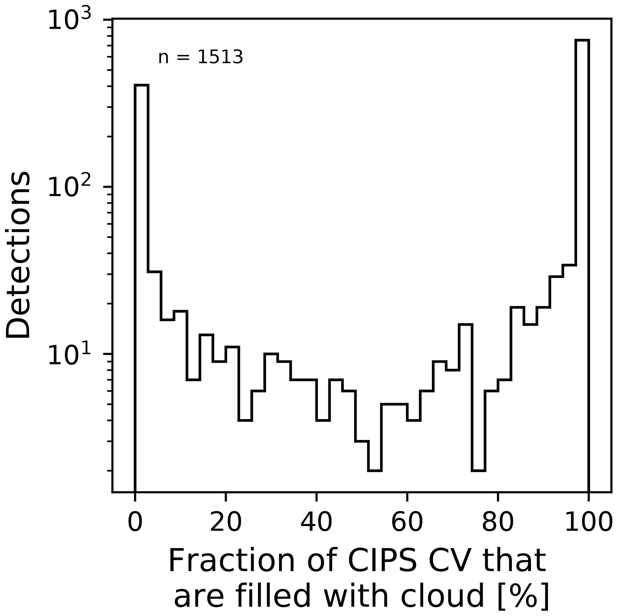
Figure 2AIM CIPS occurrence of PMCs in the common volume with OSIRIS during the observations in 2010–2011. The plot shows the number of CVs containing a certain fraction of CIPS pixels with identified PMCs. Average latitude is 80∘ N, local time . The mean cloud fraction is 62 %.
3.3 Method to make limb and nadir observations comparable in the common volume
Recently, Benze et al. (2018) demonstrated a method for comparing PMC observations from the normal (non-tomographic) OSIRIS limb scans to CIPS. This method took into account the measurement geometry and instrument sensitivity. By performing a detailed common volume comparison, their study showed that the PMC brightness from the normal OSIRIS scans agrees well on average ( %) with the CIPS brightness. The method for the PMC satellite comparison described in their study provides the basis for the comparison method in the current study. However, some important modifications are necessary for the more detailed tomography comparison.
When comparing observations from two instruments with different viewing geometry and resolution it is necessary to both define the appropriate common volume and make the observational quantities comparable. The signal from each satellite needs to be integrated to fill the common volume. The primary PMC product of OSIRIS is the volume scattering coefficient (m−1 sr−1), while the primary PMC product of CIPS is directional albedo at 90∘ scattering angle (sr−1). The OSIRIS volume scattering coefficient has a coarse horizontal resolution, but a high vertical resolution, while the CIPS albedo has a high horizontal resolution but no vertical resolution (Table 2). To make these two quantities of PMC cloud brightness comparable, one needs to define a common quantity in the common volume that accounts for the difference in vertical and horizontal resolution.
Since the OSIRIS tomographic PMC products are reported on a vertical–horizontal plane with the vertical axis as altitude (rather than tangent altitude as for the normal OSIRIS PMC retrievals), βλ can be converted into albedo (A) and measured per steradian (sr−1) by integrating over the vertical column, assuming optically thin clouds. To clarify, we integrate the OSIRIS scattering coefficient vertically to answer the question of what albedo would CIPS retrieve from the same PMC volume? The resulting albedo from OSIRIS can be expressed as Eq. (2):
where the vertical integration limits of 76 and 90 km are given by the vertical extent of the tomographic dataset, and β277 nm is the retrieved volume scattering coefficient at the wavelength 277 nm.
Albedo at a scattering angle of 90∘ for CIPS in the common volume element (x, y) is defined as Eq. (3):
where 90∘ refers to the scattering angle that CIPS albedo observations are normalized to, and 265 nm refers to the region of the spectrum where CIPS operates.
The two quantities, AOSIRIS and ACIPS, cannot be compared directly since the satellites observe the PMCs in different parts of the UV range and observe the clouds under different scattering conditions. The next section describes how this is handled to make the observations comparable in the common volume elements.
As mentioned earlier, OSIRIS observes PMCs and the background atmosphere at wavelengths between 275 and 810 nm with a resolution of about 1 nm, while CIPS observes PMCs in a wavelength region centred at 265 nm with a width of 15 nm. The tomographic retrieval provides the local scattering coefficient for seven wavelength intervals in the UV (centred at 277.3, 283.5, 287.8, 291.2, 294.4, 300.2 and 304.3 nm; also see Table 1 in Karlsson and Gumbel, 2005) and uses these to retrieve the microphysical properties. The reported CIPS albedo is normalized to a solar scattering angle of 90∘, while the OSIRIS local scattering coefficient in the overlapping volume is measured at solar scattering angles between 75 and 78∘. To make the two quantities comparable, a correction for the differences in scattering conditions and wavelengths is necessary. In this study, we convert CIPS albedo into the conditions used for OSIRIS. The conversion factors depend on the PMC scattering properties and thus on the size and shape of the PMC particles. In this study, we base our conversion factors on the particle sizes retrieved from CIPS, using the same assumptions as in the operational CIPS retrievals, namely that the particles consist of water ice, that the particle shape is oblate spheroids with axial ratio 2 and that the particle size distribution is a normal distribution with width varying as a function of mode radius as up to rm=40 nm and approximately constant above (Baumgarten et al., 2010; Lumpe et al., 2013). The conversion factors are obtained from numerical T-matrix simulations (Mishchenko and Travis, 1998). The conversion factor that corrects for solar scattering angle (SSA) differences Cphase ranges between 0.39 and 5.57 for particles between 1 and 100 nm. Cphase increases with increasing particle size. For particles in the range 1–20 nm Cphase varies between 1.0 and 1.5, for 21–50 nm Cphase varies between 0.6 and 2.7 and for particles in the range 51–100 nm Cphase varies between 0.4 and 5.6. The spectral conversion factor Cspectral range between 0.8 and 1.0.
Each CIPS pixel is transformed into scattering conditions of OSIRIS by multiplication of the conversion factors Cspectral and Cphase corresponding to the retrieved CIPS radius in the same pixel and subsequently averaged over the CV element to generate a mean albedo comparable to OSIRIS. The mean CIPS albedo in the CIPS CV element can be expressed as Eq. (4):
When comparing OSIRIS and CIPS data, these conversion factors introduce an additional uncertainty, beyond the specific uncertainties of the OSIRIS and CIPS datasets. These uncertainties will be discussed in Sect. 4.1. As noted in Sect. 2.2.1, we manually set all dim CIPS pixels sr−1 to zero in the qualitative comparison. These zero pixels have been included in the average of CIPS mean albedo.
Besides comparing the cloud albedo between the instruments, we also extend our study by comparing the cloud ice. While OSIRIS tomography reports cloud ice as ice mass density (IMD) in units of (ng m−3), CIPS reports the column-integrated quantity ice water content in units of (µg m−2). To make these two quantities comparable in the common volume element, we adopt the same integration method as for comparing albedo described in the section above. The OSIRIS IWC can be calculated from a vertical integration of OSIRIS IMD following Eq. (5):
The appropriate CIPS value of IWC is the mean value of IWC in all pixels in the CV element, including all the ice-free pixels following Eq. (6):
The microphysical properties IWCOSIRIS and IWCCIPS are directly comparable – in contrast to albedo, no transformation factors are necessary for the comparison.
3.4 Subset selection
The statistical analysis of albedo is based on 180 coinciding satellite orbits from NH 2010 and NH 2011. Out of these 180 orbits, 2 OSIRIS orbits from NH 2010 had to be discarded due to geolocation errors. For each common volume observation, approximately 14 CV element observations with CIPS are performed, making a total of approximately 2492 possible CV element observations available for the statistical analysis for the 2010 and 2011 seasons. The coarser horizontal resolution of OSIRIS requires the application of appropriate averaging to the CIPS data before a comparison of retrieved cloud properties is feasible. As discussed in Sect. 2.1, the OSIRIS averaging kernel can be represented by a Gaussian distribution with FWHM of 280 km. As a consequence, each comparison between CIPS and OSIRIS requires the CIPS data to be averaged over several of the common volume elements of size 55 km × 30 km. On the edges of the CIPS orbit strip, this demand puts restrictions on the number of CIPS common volume elements that can be included in the comparison, reducing the available number of common volume elements per OSIRIS orbit from 14 to approximately 10 and the total number of common volume elements from 2492 to ∼1500. Limiting the statistical analysis to common volume elements containing only good quality pixels based on CIPS quality flags (discussed in the section “Discussion of CIPS PMC uncertainties”) further reduces the number of common volumes to 1292.
We have performed a statistical analysis of albedo and IWC between OSIRIS and CIPS in the common volume. To gain deeper insight into the relationship between both datasets, we have also compared albedo and IWC along single orbits. The previous section described the coincidence criteria and the method for making the PMC data from OSIRIS and CIPS comparable in the common volume. The cloud properties from each instrument are made comparable in the common volume by integrating the OSIRIS local scattering coefficient and IMD vertically and taking the horizontal mean of the CIPS albedo and IWC. In addition, as described in the previous section, the CIPS albedo is transformed into the scattering conditions of OSIRIS. A coincidence criterion of 5 min has been applied, and a preliminary selection based on the quality flag has been performed to eliminate questionable data pixels. This section is divided into two different parts, starting with the statistical comparison of albedo and IWC and the uncertainties related to the choice of comparison method used in this study in Sect. 4.1. In Sect. 4.2 we present the results from the individual orbits.
4.1 Quantitative comparison of OSIRIS albedo with CIPS
Figure 4 shows a scatter plot comparing the OSIRIS albedo and CIPS albedo in the common volume for the total set of 1292 observations. Each dot represents the albedo inferred from OSIRIS and the corresponding albedo inferred from CIPS in the common volume element, and the grey dashed line denotes the one-to-one line. Figure 4 shows that OSIRIS albedo and CIPS albedo generally agree well both for faint clouds and bright clouds, although for most cases, OSIRIS albedo is higher than CIPS. We determine the offset between the OSIRIS and CIPS albedo results as sr−1 ( sr−1). The uncertainty of this offset has been estimated based on the errors of the individual OSIRIS and CIPS albedos in Fig. 4. As a limb-viewing instrument, OSIRIS observes PMCs as enhancements in the limb radiance and integrates the signal over a long distance, while CIPS as a nadir instrument observes PMCs as enhancements in the brighter Rayleigh background and integrates the signal over a much shorter distance. OSIRIS can, therefore, observe fainter clouds than CIPS. To quantify the agreement between the instruments for various cloud regions, we sort the observations into three regions based on OSIRIS albedo: faint clouds (0– sr−1), medium bright clouds (10– sr−1) and bright clouds (30– sr−1), and we calculate the Pearson correlation coefficient for each region. For faint clouds the correlation is 0.81, for medium bright clouds the correlation is 0.85, and for bright clouds the correlation is 0.92. The correlation coefficient for the total set of observations is calculated to be 0.97. The small systematic bias of sr−1 ( sr−1) between CIPS and OSIRIS together with an overall correlation coefficient of 0.97 for the 1292 CV elements shows a very good agreement between the instruments and analysis methods.
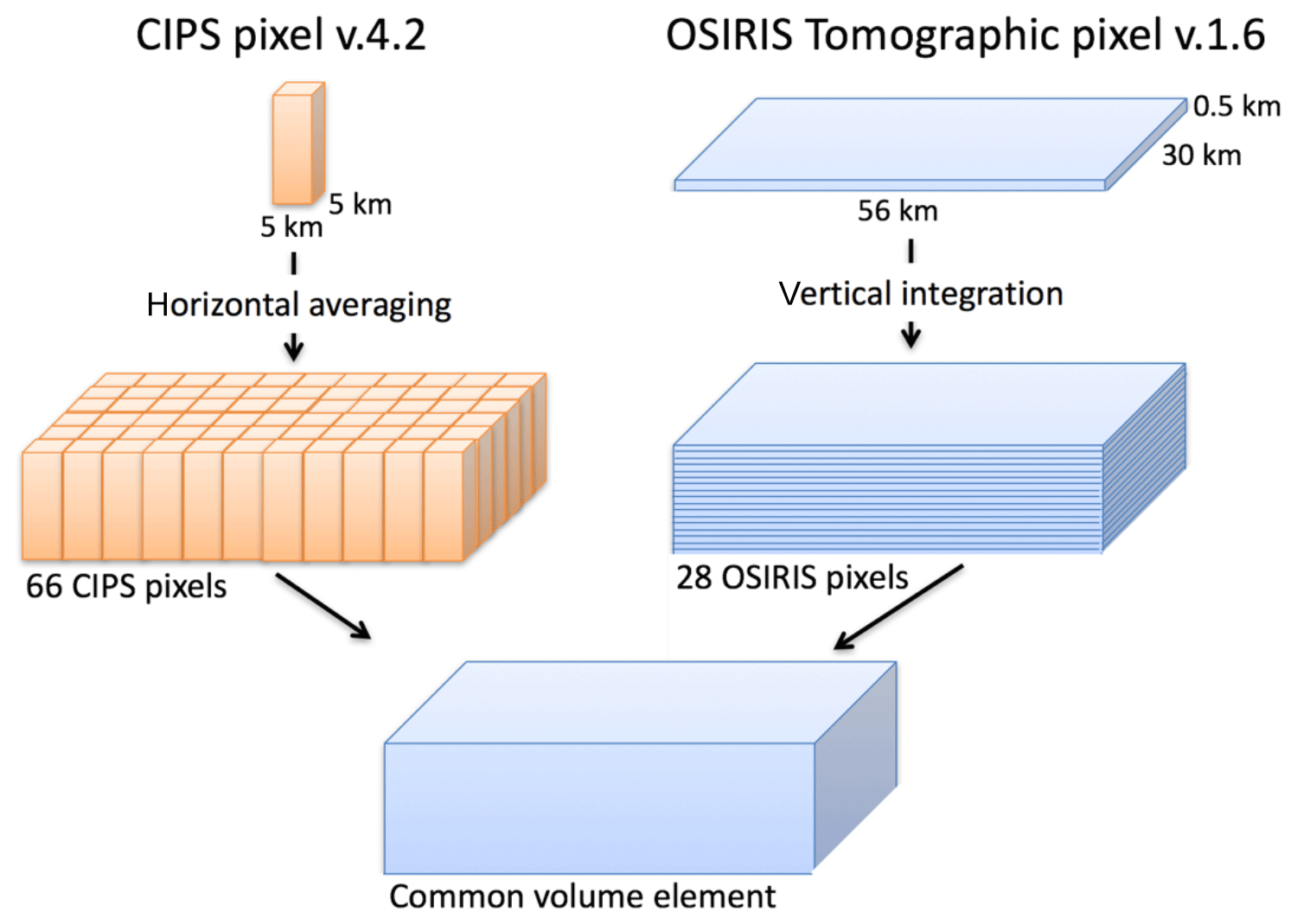
Figure 3The 3-D common volume is defined by the horizontal extent of one OSIRIS tomographic pixel (56 km×30 km) and the vertical range (76 to 90 km) of the OSIRIS tomography observations. CIPS pixels have a size of 25 km2 with each side 5 km in the nadir. In order to make CIPS comparable to OSIRIS in the CV, 66 CIPS pixels (11×6) are averaged over the CV. The tomographic OSIRIS pixels need to be integrated over the column of 28 levels to be comparable to CIPS.
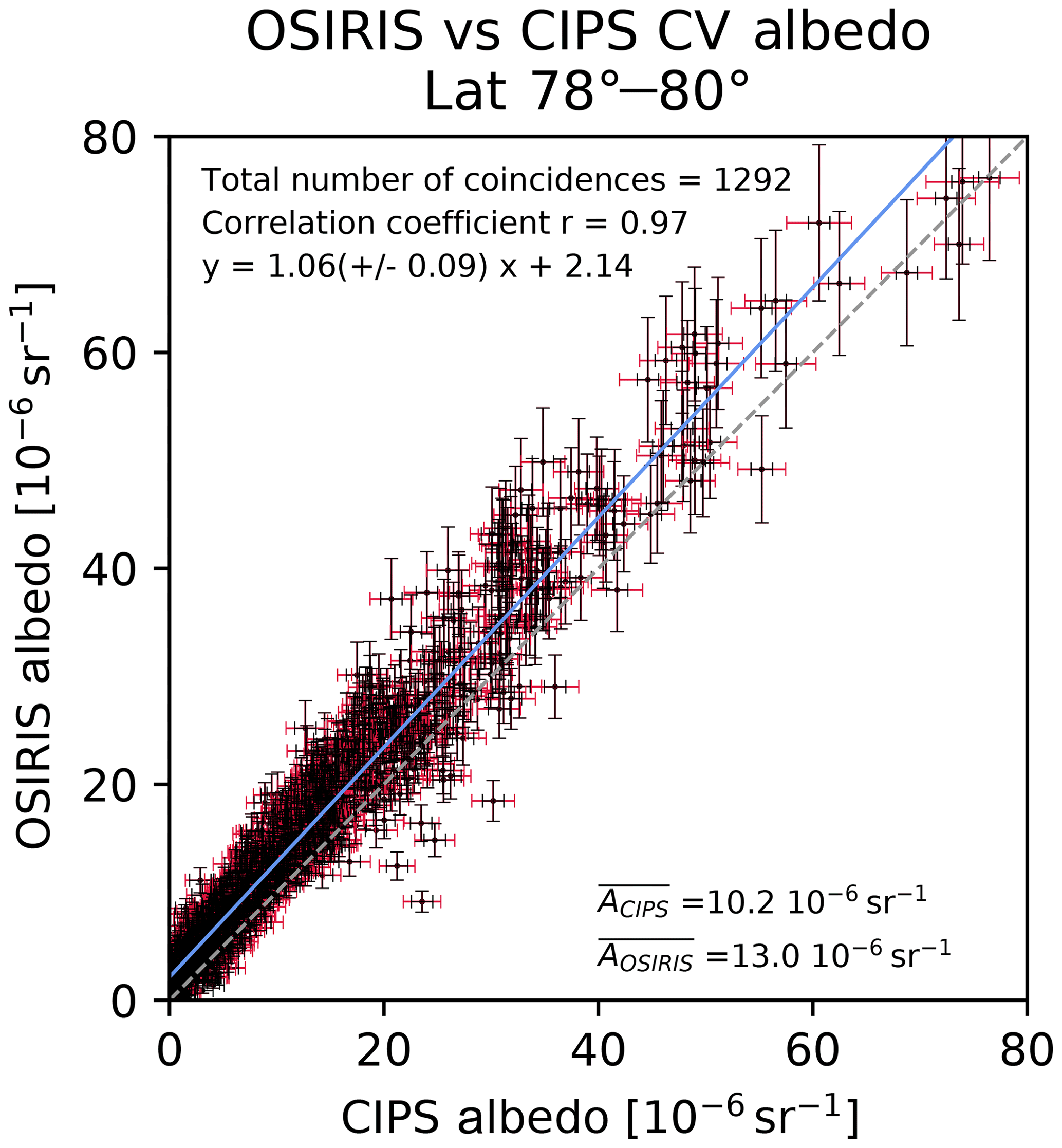
Figure 4Scatterplot of OSIRIS and CIPS observations of albedo in the common volume. The grey dashed line denotes the one-to-one line. The blue line is the regression line. The average albedo for CIPS and OSIRIS for all the CV in the figure is indicated in the bottom right of the figure. OSIRIS error bars are a combination of systematic and statistical uncertainty. CIPS error bars are a combination of statistical uncertainty and uncertainty due to handling of dim cloud pixels (black), while the extended error bars (red) denote the uncertainty that is introduced by conversion factors that accounts for the difference in wavelength and scattering angle between the instruments. The reader is referred to the error discussion in the text for a more detailed description of CIPS and OSIRIS errors.
The error bars in Fig. 4 represent the error from the basic uncertainty discussed in detail in section “Discussion of OSIRIS tomography uncertainties” (OSIRIS) and section “Discussion of CIPS PMC uncertainties” (CIPS), combined with the error that is introduced by transforming the data into a comparable property in the CV. For OSIRIS, the directional albedo is, as previously mentioned, obtained as the vertical column integral over the scattering coefficients. In order to represent the uncertainty of the column albedo caused by this integration, the error bars of the albedo include the root of the sum of the squares of both the systematic error (10 % due to calibration) and the estimated random error of the scattering coefficient described in Sect. 2. The resulting error of the OSIRIS albedo is dominated by the uncertainty of the brightest PMC pixels in the column. For dim or PMC-free areas, the albedo error is essentially determined by the PMC retrieval threshold at each altitude, which sums up vertically to about sr−1. This number can be interpreted as a PMC detection threshold of OSIRIS expressed in terms of directional albedo.
For CIPS, the directional albedo is obtained as the horizontal average of the pixels contained in the CV element. The corresponding uncertainty is a combination of the uncertainty due to the conversion factors, a statistical uncertainty (of sr−1) and an uncertainty due to the handling of dim cloud pixels. The following text describes how these CIPS uncertainties are handled in our study. As described in Sect. 3.3, conversion factors must be applied in order to make the observation conditions of OSIRIS and CIPS comparable. Cspectral accounts for the difference in wavelengths, Cphase accounts for the difference in scattering angle. These factors depend on the particle size and are calculated based on the CIPS size retrievals. They introduce an additional uncertainty to the OSIRIS/CIPS albedo comparison, beyond the specific uncertainties of both datasets. This uncertainty can be assessed based on the uncertainty of the CIPS particle size retrieval. Lumpe et al. (2013, Fig. 21) discuss the CIPS radius uncertainty as a function of PMC albedo and solar zenith angle. We thus obtain an uncertainty of the conversion factors by applying these radius uncertainty ranges when calculating the conversion factors from our T-matrix approach. The resulting uncertainties of the conversion factors are included as additional error bars in the CIPS data, marked in red in Figs. 4 and 6. Note that these red error bars do not denote uncertainties inherent to CIPS but uncertainties of our OSIRIS/CIPS comparison method. In order to represent the uncertainty of the mean CIPS albedo caused by the horizontal averaging over all the CIPS pixels in the common volume element, it is necessary to consider the handling of CIPS dim pixels in the current study. By manually setting all CIPS pixels where albedo sr−1 to 0, an additional statistical uncertainty is introduced to the mean CIPS albedo. This uncertainty can be easily tested by setting the albedo in these CIPS pixels to either 0 (lower limit) or sr−1 (upper limit). It turns out that the resulting uncertainty range of the mean CIPS albedo varies linearly with albedo for the dim clouds. A linear fit then provides an expression of this “dim cloud” uncertainty as a function of albedo. In the albedo range of 0– sr−1, the resulting error due to “dim clouds” can be represented as CIPS mean albedo +2.5, and 0 for CIPS mean albedo sr−1. The slope is −0.2 and the intercept is +2.5. The black error bars in Figs. 4 and 6 represent the square sum of the statistical uncertainty and the uncertainty due to the dim clouds while the red error bars represent the uncertainty that is caused by the conversion factors.
4.1.1 Accounting for differences in sensitivity
To further analyse the albedo bias between the instruments and to quantify the contribution from different sources it is useful to again consider how the dim pixels are treated in the CIPS retrieval. The CIPS sensitivity to faint clouds has been quantified by Lumpe et al. (2013) and is shown in their Fig. 18. The sensitivity to faint clouds is strongly dependent on solar zenith angle and the detection rate is highest for high SZA and declines for lower SZA, especially for the faint clouds. The SZA during the date and time for the tomographic scans in 2010 and 2011 is around 60∘. For this SZA, the detection rate for sr−1 clouds is 40 %, for sr−1 clouds 70 % and for sr−1 clouds 90 % (Lumpe et al., 2013). Since it is likely that CIPS reports zero cloud in the pixels where it is not able to detect clouds, the fraction of pixels in the CV element that is filled with non-zero albedo (fill factor) will inevitably affect the albedo comparison between the instruments for the faint clouds. Figure 5 compares the relative disagreement in cloud albedo between the instruments. Each dot represents the relative difference vs. CIPS albedo and is colour-coded by the percentage of non-zero pixels in the CIPS CV element. As can be seen from this figure, the instruments tend to disagree when the percentage of non-zero pixels decreases. For the CV elements that have a large number of dim CIPS pixels, the mean albedo for this CV element will be underestimated. The instruments agree best for bright clouds, but for faint clouds, especially where CIPS reports a mean albedo sr−1, the agreement is worse. It is also clear from Fig. 5 that for dim CIPS clouds that have a large disagreement with OSIRIS, the fill factor is small (purple colour). Benze et al. (2018) evaluated the dependence of the percentage filling of the CIPS CV and showed that the sensitivity issue could be avoided using a threshold on the fill factor of 95 %. It is thus appropriate to apply a threshold on the CIPS CV fill factor in the current study, and for consistency with Benze et al. (2018) we use the value of 95 %. To summarize, the following two sensitivity adjustments are applied to CIPS pixels: (1) all pixels with an albedo sr−1 are set to zero; (2) a filling factor of 95 % is required, meaning that only CIPS CVs with at least 95 % cloud pixels are included in the comparison. This also includes those faint pixels that were set to zero in the previous step. The few remaining non-cloud pixels are included in the horizontal average.
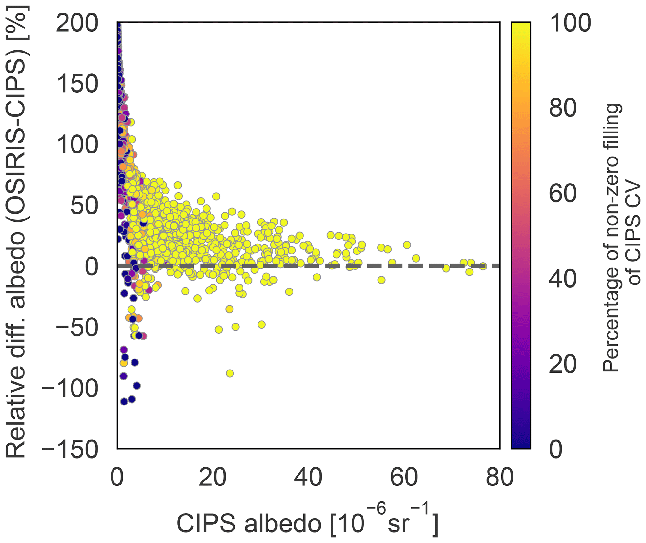
Figure 5Relative difference in cloud albedo in CV elements (2× (OSIRIS-CIPS)∕(CIPS + OSIRIS)) vs. CIPS albedo. The points are colour-coded by the percentage of filling of non-zero pixels in a CIPS CV element.
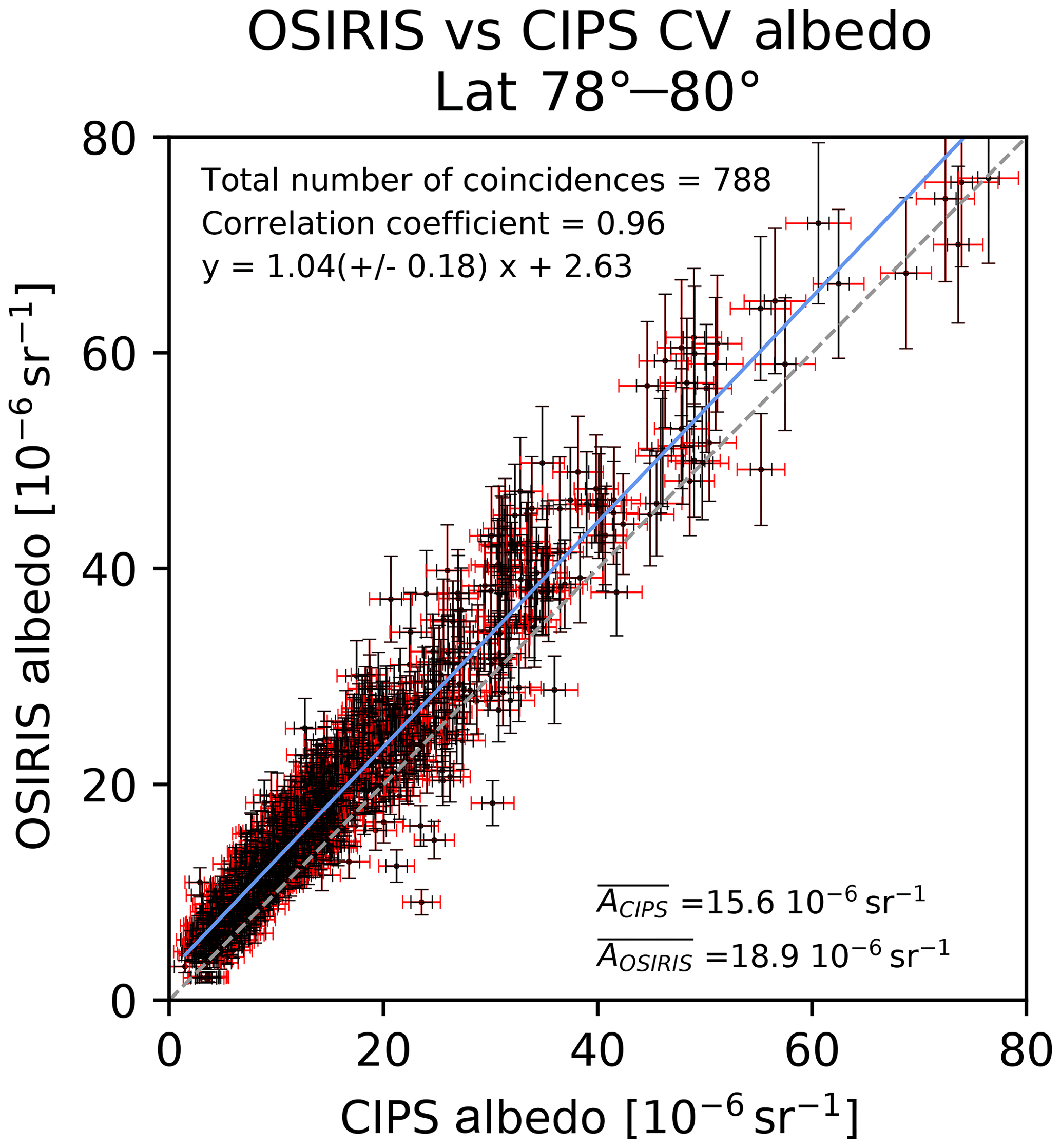
Figure 6Scatterplot of OSIRIS and CIPS mean albedo in the CV. Same as Fig. 4, but using thresholds on CIPS fill factor of 95 % and an OSIRIS scatter coefficient threshold of 10−10 m−1 sr−1 as discussed in the text. The average albedo for CIPS and OSIRIS for all the CV in the figure is indicated in the bottom right of the figure. The grey dashed line denotes the one-to-one line. The blue line is the regression line.
To account for the differences in sensitivity, we additionally apply a retrieval threshold on the OSIRIS cloud scattering coefficient of 10−10 m−1 sr−1 (as discussed in Sect. 2) when vertically integrating the cloud scattering coefficient to retrieve mean albedo in the CV. All vertical levels that have a cloud scattering coefficient below the retrieval threshold will not be included in the vertical integral. Figure 6 shows a scatterplot comparing OSIRIS albedo and CIPS albedo in the common volume if we apply a fill factor threshold of 95 % to CIPS CV elements and apply a retrieval threshold of 10−10 m−1 sr−1 to the OSIRIS scattering coefficient (figure layout is the same as Fig. 4). The total number of observations decreases from 1292 to 788 due to the restriction of the filling of the CIPS CV element. Accounting for the differences in sensitivity and adding a threshold on CIPS fill factor of 95 % improves the agreement between the instruments for the faint clouds. However, OSIRIS is more sensitive to smaller ice particles than CIPS, and it is possible that some of the ice that is detected by OSIRIS as faint clouds comes from clouds with small ice particles that are below the CIPS detection threshold. Some difference in the observed albedo quantities is therefore expected. With the discussed changes the observed discrepancy between the instruments increases from sr−1 ( sr−1) (Fig. 4) to sr−1 ( sr−1) (Fig. 6) and the correlation coefficient decreases from 0.97 to 0.96.
4.1.2 Quantitative comparison of OSIRIS IWC with CIPS
Figure 7 shows a scatterplot comparing OSIRIS and CIPS IWC in the common volume for a total set of 788 common volume element observations. Each dot represents the IWC inferred from OSIRIS and the corresponding IWC from CIPS in the CV element. The systematic uncertainty of CIPS IWC strongly increases with decreasing particle size. As described in Sect. 2.2.1, we take this into account by screening out the suspicious IWC detections, only including CIPS pixels that report a particle radius >20 nm when we calculate the mean IWC in each CV element. For consistency with the albedo comparison, we have applied a CV fill threshold of 95 %. For OSIRIS, the retrieval threshold (10−10 m−1 sr−1) is applied in the vertical integration to form IWC in the common volume by vertically integrating the IMD at each level. We find an offset between OSIRIS and CIPS IWC, and we quantify this offset (OSIRIS - CIPS) to g km−2.
The error bars in Fig. 7 represent a total error that is relevant for the comparison between the instruments by combining systematic and statistical error from each dataset. Based on the discussion in the section “Discussion of OSIRIS tomography uncertainties”, the OSIRIS error bars combine the absolute uncertainty of IMD due to the 10 % measurement accuracy and a statistical uncertainty that is obtained by propagating the uncertainty of the scattering coefficient through the derivation of the IMD at each level. The resulting error in IWC in the common volume element is calculated in the column integration as the combined error of IMD from all vertical levels. Similarly, the CIPS error bars (in grey) represent the systematic and statistical uncertainty propagated from all individual CIPS pixels in the CV element. The individual uncertainty for each pixel is taken from Fig. 21 in Lumpe et al. (2013), where both the estimated systematic uncertainty and the statistical uncertainty of CIPS IWC are given as a function of IWC and particle radius for different ranges of solar zenith angles. For the range of solar zenith angles in our study (59 to 71∘), the systematic uncertainty for medium (40–60 nm) and large (60–80 nm) particles is between −5 and −10 g km−2, while for smaller particles (20–40 nm) the systematic uncertainty is between −5 and −35 g km−2. In addition to the systematic uncertainty, the statistical uncertainty (standard deviation) for medium (40–60 nm) and large particles (60–80 nm) is between 5 and 10 g km−2 and for smaller particles (20–40 nm) the statistical uncertainty is between 15 to 40 g km−2. Especially for small particles, the statistical uncertainty is highly dependent on IWC.
Unlike for the albedo comparison (Figs. 5 and 6), where correction factors for phase and wavelength are applied, no corrections are needed for the comparison of IWC in the CV element, and hence no additional error bars for this conversion are needed. Generally, CIPS and OSIRIS IWC observations agree well within the common volume. The relative difference is large for the dimmest clouds and decreases for stronger clouds. The correlation coefficient is calculated to be 0.91 between the instruments.
4.2 Orbit-wise comparison of OSIRIS albedo with CIPS
The results from the above statistical comparison show that the instruments agree very well on average, that the choice of method used for the instrument comparison is valid, and that the time constraint and size of the common volume are suitable. In this section, we continue to compare the instruments using the individual strengths of each instrument, i.e. the horizontally resolved CIPS data and the vertically resolved OSIRIS data. As described in Sect. 2.1, the ability of OSIRIS to resolve individual cloud structures varies stochastically. As the number of measurements along the orbit is sparse, the resolution depends on the placement of lines of sight relative to the actual cloud structure. Therefore, when comparing CIPS data to the OSIRIS tomography in this section, we apply a horizontal integration of the CIPS data of both 56 km (size of OSIRIS retrieval pixel) and 280 km (typical OSIRIS averaging kernel) as limiting cases.
We present the observations of cloud brightness from three individual OSIRIS orbits and the coinciding CIPS orbits in Figs. 8, 9 and 10. These particular orbits were chosen to illustrate some examples of when the cloud in the CV show good agreement, and point out one example when the cloud observations in the CV disagree and thus illustrate for the reader the range of cloud observations available for this study. Figs. 8a, 9a and 10a show the vertically and horizontally resolved OSIRIS scattering coefficient for the subset of the orbit that overlaps the coinciding CIPS orbit strip. The abscissa is given in OSIRIS AAO and the vertical axis covers the subrange 78–88 km. Figs. 8b, 9b and 10b show CIPS albedo for the subset of pixels that overlap the OSIRIS field of view along the OSIRIS line of sight. The horizontal pink lines mark the width of the OSIRIS field of view, and the CIPS pixels within these lines denote the pixels within the CV. Note that this plot is not the normal CIPS orbit strip image that uses polar projection map, but only the subset of pixels in the CIPS CV level 2 geolocated data that we have plotted on a new grid to facilitate a comparison using the same abscissa. The region in close proximity (±30 km, i.e. ±6 CIPS pixels) to the CIPS common volume is included in this figure for illustrative purposes. The abscissa in panel (b) is given in CIPS pixels along OSIRIS LOS and is hence identical to the abscissa in panel (a). Panel (c) shows the resulting albedo in the CV for each instrument given in the unit G and along the abscissa AAO. The black line shows the mean OSIRIS albedo in the common volume corresponding to the scattering coefficient in the first panels. The green line shows the mean CIPS albedo in the common volume when a horizontal integration of 56 km is applied (high-resolution limit) and the turquoise line shows the mean CIPS albedo in the common volume when a horizontal integration of 280 km is applied (low-resolution limit).
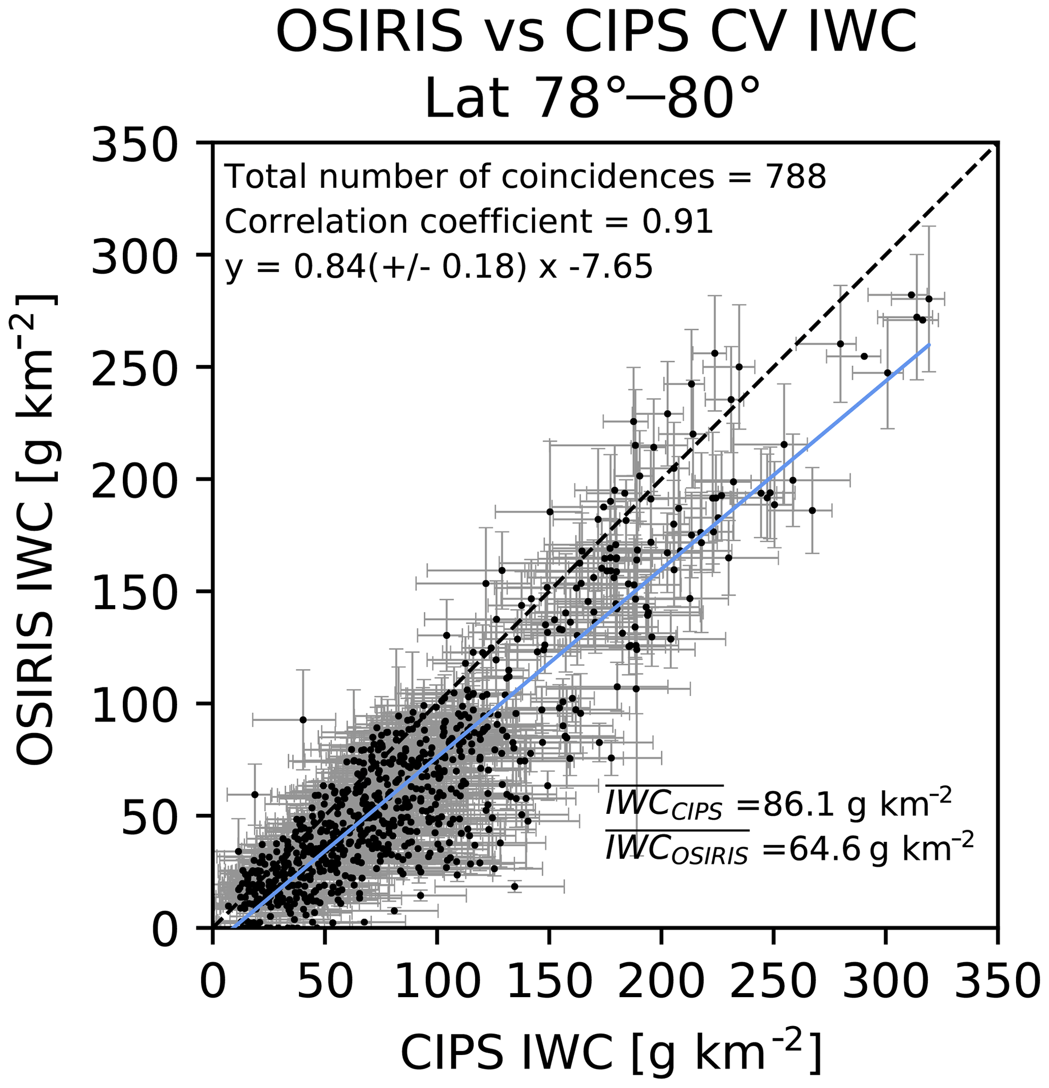
Figure 7Scatterplot of OSIRIS and CIPS common volume ice water content. The average IWC for CIPS and OSIRIS is indicated in the bottom right of the figure. The error bars are a combination of the systematic and statistical uncertainty from each instrument, thus representing a total uncertainty that is relevant when comparing the datasets. The grey dashed line denotes the one-to-one line. The blue line is the regression line.
For OSIRIS orbit 51236 (Fig. 8) observed during 16 July 2010, a bright continuous cloud layer is visible between approximately 82.5 and 85 AAO, with the brightest region of the cloud at 84–84.5 AAO and at altitude ∼83.5 km. Simultaneously, the coinciding CIPS orbit 17556 observes the same bright cloud layer, although the higher horizontal resolution of CIPS makes it possible to detect the bright cloud region at 83.5 AAO. The higher horizontal resolution of CIPS makes it possible for this instrument to clearly distinguish this bright cloud region even when averaged over the horizontal extent of one CV, which can be seen by the peak of sr−1 at 83.5 AAO in panel (c). Applying the averaging kernel to CIPS (and thus “smoothing” the data to OSIRIS resolution) produces a mean albedo of sr−1 in the same cloud region, very close to the OSIRIS albedo of sr−1. Comparing the mean albedo from CIPS and OSIRIS in this orbit confirms the good agreement concerning both the absolute value of the peak albedo and the spatial variations of the albedo throughout the extent of the overlapping cloud volumes.
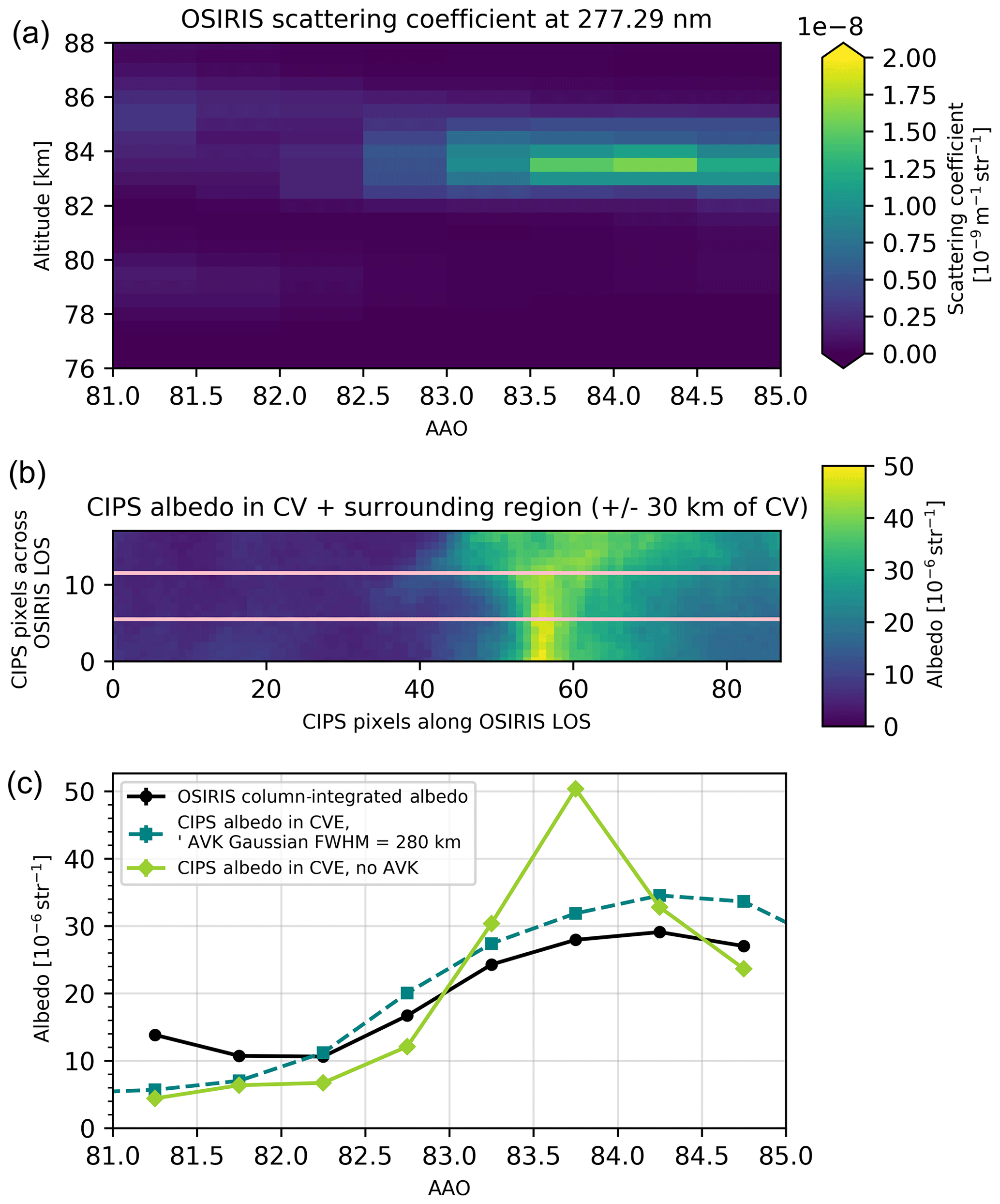
Figure 8Common volume observations of cloud albedo for OSIRIS orbit 51236 and CIPS orbit 17556. The coincidence occurs at latitude 78∘ N and longitude 150∘ at 15:45 LT. Panel (a) shows the OSIRIS cloud scattering coefficient (vertical plane) for the subset of the orbit that overlaps CIPS orbit strip. Panel (b) shows CIPS albedo (horizontal plane) for the subset of pixels that overlap the OSIRIS field of view along OSIRIS LOS. The pink lines denote the width of OSIRIS LOS, and consequently the CIPS pixels within the pink lines that are contained in the CV. The region ±30 km outside the CV is included only for illustrative purposes. The abscissa in (b) is given in CIPS pixels along OSIRIS LOS and is hence identical to the abscissa in (a). Panel (c) shows the resulting albedo in the CV for the integrated signal from each instrument along the abscissa AAO.
For OSIRIS orbit 50796 (Fig. 9) observed on 17 June 2010, a cloud layer is visible between 81 and 83 AAO, with the brightest cloud layer at an altitude of 85 km at 81.5 AAO. Coinciding CIPS orbit 17117 shows a cloud in the same region that is highly structured in the CV. By comparing the mean albedo in the CV, we note that OSIRIS albedo is 2– sr−1 higher than CIPS (before applying the averaging kernel) throughout the whole CV. The observed differences for this orbit are larger than the estimated error bars.
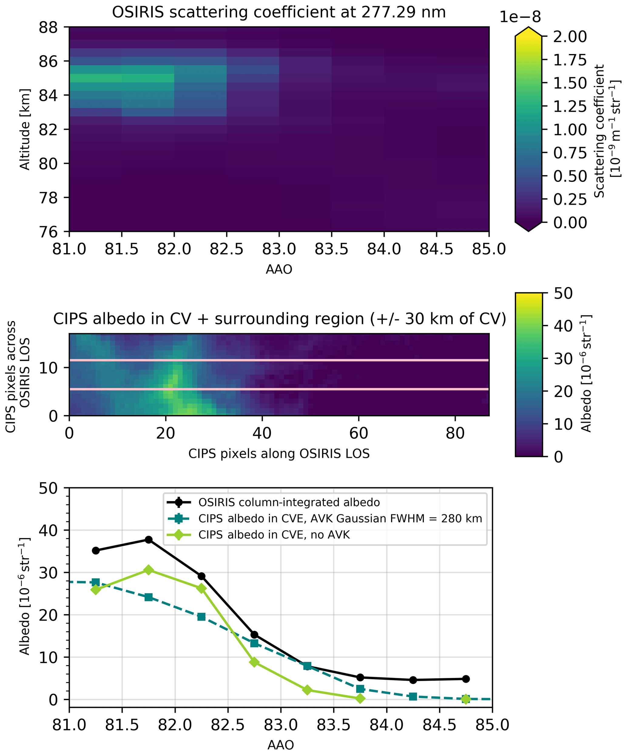
Figure 9As in Fig. 8, but for OSIRIS orbit 50796 and CIPS orbit 17117. The coincidence occurs at latitude 79∘ N and longitude 305∘ at 15:45 LT.
For OSIRIS orbit 51646 (Fig. 10) taken during 16 July 2010, a bright cloud layer with a vertical extent of ∼4 km encompasses the whole CV from AAO 81 to 85. The brightest cloud region is found at an altitude of 84.5 km at AAO 82.5. Simultaneously, the coinciding CIPS orbit 17965 observes the same bright cloud layer, but additionally reveals that this cloud layer is highly structured. The brightest cloud layer observed by CIPS is located at 83–83.5 AAO. In this orbit, the resulting mean albedos do not show good agreement, and an apparent horizontal shift between OSIRIS and CIPS is noteworthy. In cases like this, with a sharp gradient across the OSIRIS LOS, a possible explanation for the discrepancy is the action of horizontal wind transporting clouds out of or into the CV. At PMC altitude the horizontal wind is mainly modulated by atmospheric tidal waves and gravity waves. Horizontal wind velocities of ∼50 m s−1 have been observed by The Middle Atmosphere Alomar Radar System (MAARSY) in northern Norway (Stober et al., 2013). In this CV, the time difference between CIPS-OSIRIS observations is ∼5 min. During this time, a wind speed of 50 m s−1 would transport a cloud 15 km, which corresponds to half the width of OSIRIS LOS. It is likely that the cloud region outside the CIPS-OSIRIS CV (as indicated by the pink lines in the third panels) could have been transported into the CV by wind directed across the OSIRIS LOS.
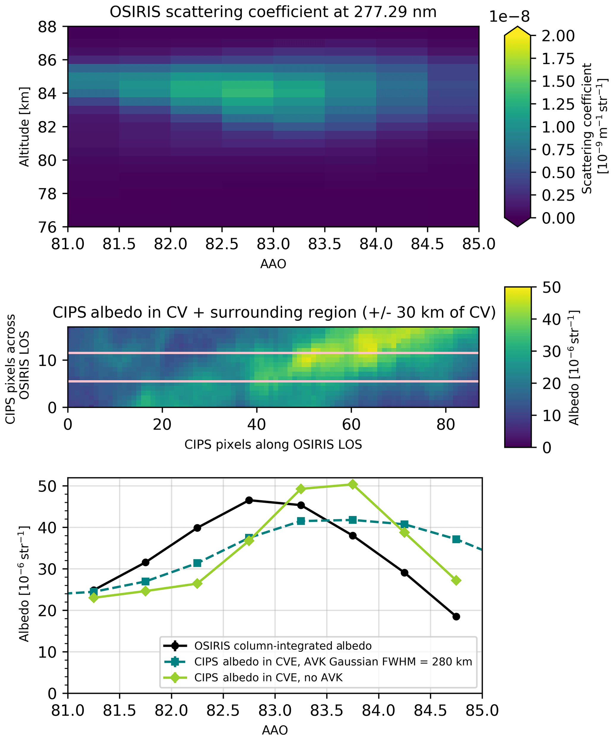
Figure 10As in Fig. 8, but for OSIRIS orbit 51646 and CIPS orbit 17965. The coincidence occurs at latitude 79∘ N and longitude 357∘ at 15:45 LT.
In this study, we have compared the PMC cloud properties cloud albedo and IWC from Odin OSIRIS limb tomography to the nadir-viewing AIM CIPS. The analysis is performed for 2010 and 2011 in the Northern Hemisphere for a total set or 180 coinciding orbits at latitudes from 78 to 80∘ N for local time. The OSIRIS tomographic PMC dataset provides combined coarse horizontal and high vertical information, while CIPS provides preeminent horizontal PMC information. When combined in a common volume study, OSIRIS can provide vertical information of structures such as double cloud layers and ice voids as well as detailed particle size and number concentration information at various height levels to the detailed horizontal PMC information from CIPS. This information can be used to study how atmospheric waves of different scales (inferred from albedo variations in CIPS) alter the vertical distribution of cloud properties (inferred from OSIRIS). Additionally to such studies, the combined CIPS/tomographic dataset OSIRIS provides useful insight into more detailed studies of the PMC particle size distribution.
First, we have extended the previous OSIRIS error description by Hultgren et al. (2013) by performing a detailed error characterization for the local cloud scattering coefficient and IMD that takes into account absorption of mesospheric ozone along the LOS. Second, we have compared these cloud properties to common volume observations from CIPS. To be able to compare the common volume cloud properties from two different satellite instruments (OSIRIS using limb geometry and adapting spectroscopy to retrieve cloud properties, and CIPS using nadir geometry and adapting multi-angle phase function observations of PMC to retrieve cloud properties), it is necessary to account for the differences in scattering conditions, observational volume and sensitivity. In this study, we have averaged the high horizontal resolution CIPS albedo and IWC to the coarser horizontal resolution of OSIRIS tomography. Additionally, we have a vertically integrated OSIRIS scatter coefficient and IMD to obtain albedo and IWC comparable to CIPS. We have accounted for the differences in scattering conditions by transforming CIPS albedo into the SSA and wavelengths used by OSIRIS. By adopting a very narrow spatial and temporal coincidence criterion, we have been able to capture a large variety of albedo and IWC in the common volume. We have shown that the OSIRIS error characterization of the volume scattering coefficient and IMD is valid by demonstrating that the cloud properties within the common volume largely agree within the specified error for each instrument analysis. We find that the OSIRIS cloud scattering coefficient shows excellent agreement with CIPS cloud albedo with a correlation coefficient of 0.96, although in the common volume OSIRIS observes brighter clouds than CIPS. The bias between the instruments is found to be sr−1 ( sr−1). The correlation is higher for bright clouds than for faint clouds. Owing to differences in instrumental design and geometry, the instruments have different sensitivity. We account for these differences by adding a threshold on CIPS CV fill factor of 95 % and a scatter coefficient threshold to OSIRIS of 10−10 m−1 sr−1 and find that this leads to a better agreement for faint cloud volumes. Additionally, we find good agreement between OSIRIS IMD and CIPS IWC, with a correlation coefficient of 0.91. However, CIPS observes more ice than OSIRIS in the common volume, and the bias (OSIRIS-CIPS) is found to be −22 g km−2 (±14 g km−2).
A reason for why OSIRIS IWC is biased low to CIPS IWC is considered to arise from how IMD is calculated in OSIRIS PMC retrieval. When calculating IWC from the vertical integration of OSIRIS IMD data, we currently only take into account retrieval pixels that are bright enough for a spectroscopic size retrieval to be feasible. It is possible that the OSIRIS analysis misses ice from weak pixels where mean radii smaller than 20 nm are reported. Such weak cloud pixels typically cover an altitude range of 1 km in the upper part of the cloud. A rough estimate of how much ice OSIRIS misses by ignoring such pixels can be given by considering how much ice can be produced when converting a typical concentration of water vapour at 86 km (e.g. 3 ppm water vapour in 2×1014 cm−3 air) into ice. Calculating this, a 1 km thick layer contributes to the overall IWC with 18 g km−2. This is more or less the difference that we see in Fig. 7 between OSIRIS and CIPS IWC. Bailey et al. (2015) compare albedo, radius and IWC in a CIPS-SOFIE CV that is located at high SZAs. These clouds occur right at the terminator, where the Rayleigh background is small and has a large slope vs. SZA. This is a difficult region to observe PMCs, as even a small error in the CIPS Rayleigh background is expected to have a large impact on the retrieved cloud products. Bailey et al. (2015) apply a justifiable correction to the CIPS background removal which brings the SOFIE and CIPS observations, specifically albedo and IWC, into better agreement than without (their Fig. 11). The present study uses cloud observations at a much more favourable SZA range (59–71∘). Here, CIPS background changes such as those found by Bailey et al. (2015) are negligible, and no CIPS background correction is necessary.
Bailey et al. (2015) show that the reported v4.2 CIPS IWC is 50 % smaller than SOFIE IWC in the common volume, but only ∼30 % smaller when correcting the CIPS background removal (their Fig. 11). In the present study, we find that CIPS IWC is 33 % (±22 %) greater than that of OSIRIS in the common volume (Fig. 7). This difference between the two studies is important because IMD is the native measurement quantity for SOFIE, which can thus be seen as a reference measurement. SOFIE uses the technique of satellite solar occultation to measure vertical profiles of limb path atmospheric transmission, and as such it is much more sensitive to small ice particles than OSIRIS. The two studies use different methods: Bailey et al. (2015) model what CIPS should observe based on SOFIE observations, whereas this study corrects for sensitivity differences and compares the horizontally and vertically averaged quantities. Another difference is that this study uses observations at more favourable SZAs and higher latitudes, therefore avoiding uncertainties of the CIPS background and containing generally brighter clouds with more ice.
We have also performed a more detailed comparison of cloud properties in individual orbits. The sample of orbits used in this study illustrates the strength of this dataset. The vertically resolved OSIRIS tomography in combination with the horizontally high resolved CIPS data provides tools to study cloud structures and how these, in turn, affect the observed cloud properties in the CV.
This study has validated the OSIRIS tomographic PMC cloud brightness and ice content against nadir-viewing CIPS observations. It has addressed the potential errors from the dataset itself, as well as errors inherent to the comparison of limb tomography and nadir PMC retrievals. Due to the limitation of a total of 18 d of observations during the seasons of the Northern Hemisphere in 2010 and 2011, we have not performed a detailed comparison of cloud frequency. A follow-up paper is planned to discuss how to best compare OSIRIS limb tomography and CIPS column-integrated data when it comes to PMC particle size retrievals.
The Odin OSIRIS tomography PMC dataset used in this article, as well as codes used for the analysis, is available upon request to Lina Broman. AIM CIPS data are available for download from the Laboratory for Atmospheric and Space Physics web page: http://lasp.colorado.edu/aim/download-data.php (AIM science team, 2018).
JG and SB presented the original idea of this study. LB designed the study, carried out the analysis and wrote the majority of the paper. SB and OMC were responsible for processing the tomographic OSIRIS data. OMC and JG performed tests of the resolution of the OSIRIS tomography. All co-authors contributed to the interpretation of the results, provided feedback and contributed equally to the improvement of the paper.
The authors declare that they have no conflict of interest.
This article is part of the special issue “Layered phenomena in the mesopause region (ACP/AMT inter-journal SI)”. It is a result of the LPMR workshop 2017 (LPMR-2017), Kühlungsborn, Germany, 18–22 September 2017.
We thank Jerry Lumpe for valuable discussion related to the CIPS retrievals. We thank Gerd Baumgarten for providing scattering data from T-Matrix calculations. We thank Matthew DeLand for the helpful discussions regarding Sect. 5. We are grateful to the two anonymous reviewers whose comments have greatly improved this paper. Odin is a Swedish-led satellite funded jointly by Sweden (SNSB), Canada (CSA), France (CNES) and Finland (TEKES). Since 2007, Odin is a third-party mission of the European Space Agency. AIM is supported by NASA Small Explorers contract NAS5-03132. We gratefully acknowledge the efforts of the entire Odin and AIM development, science, and operations teams.
The article processing charges for this open-access publication were covered by Stockholm University.
This paper was edited by Andreas Engel and reviewed by two anonymous referees.
AIM science team: AIM CIPS PMC Level 2 Data v4.20r06, available at: http://lasp.colorado.edu/aim/download-data.php, last access: 18 August 2018.
Backhouse, T. W.: The luminous cirrus clouds of June and July, Meteorol. Mag. 20, 133 pp., 1885.
Bailey, S. M., Thomas, G. E., Rusch, D. W., Merkel, A. W., Jeppesen, C. D., Carstens, J. N., ... Russell, J. M. III.: Phase functions of polar mesospheric cloud ice as observed by the CIPS instrument on the AIM satellite, J. Atmos. Sol.-Terr. Phy., 71(3-4), 373–380, https://doi.org/10.1016/j.jastp.2008.09.039, 2009.
Bailey, S. M., Thomas, G. E., Hervig, M. E., Lumpe, J. D., Randall, C. E., Carstens, J. N., Thurairajah, B., Rusch, D. W., Russell III, J. M., and Gordley, L. L.: Comparing nadir and limb observations of polar mesospheric clouds: the effect of the assumed particle size distribution, J. Atmos. Sol.-Terr. Phy. 127, 51–65, https://doi.org/10.1016/j.jastp.2015.02.007, 2015
Baumgarten, G., Fiedler, J., Lübken, F.-J., and von Cossart, G.: Particle properties and water content of noctilucent clouds and their interannual variation, J. Geophys. Res., 113, D06203, https://doi.org/10.1029/2007JD008884, 2008.
Baumgarten, G., Fiedler, J., and Rapp, M.: On microphysical processes of noctilucent clouds (NLC): observations and modeling of mean and width of the particle size-distribution, Atmos. Chem. Phys., 10, 6661–6668, https://doi.org/10.5194/acp-10-6661-2010, 2010.
Baumgarten, G., Chandran, A., Fiedler, J., Hoffmann, P., Kaifler, N., Lumpe, J., Merkel, A., Randall, C., Rusch, D., and Thomas, G.: On the horizontal and temporal structure of noctilucent clouds as observed by satellite and lidar at ALOMAR (69N), Geophys. Res. Lett., 39, L01803, https://doi.org/10.1029/2011GL049935, 2012.
Benze, S., Randall, C. E., DeLand, M. T., Thomas, G. E., Rusch, D. W., Bailey, S. M., Russell III, J. M., McClintock, W. E., Merkel, A. W., and Jeppesen, C. D.: Comparison of polar mesospheric cloud measurements from the cloud imaging and particle size experiment and the solar backscatter ultraviolet instrument in 2007, J. Atmos. Sol.-Terr. Phy., 71, 365–372, https://doi.org/10.1016/j.jastp.2008.07.014, 2009.
Benze, S., Randall, C., DeLand, M., Thomas, G., Bailey, Russell, J., and Merkel, A.: Evaluation of AIM CIPS measurements of Polar Mesospheric Clouds by comparison with SBUV data, J. Atmos. Sol.-Terr. Phy., 73, 2065–2072, https://doi.org/10.1016/j.jastp.2011.02.003, 2011.
Benze, S., Gumbel, J., Randall, C., Karlsson, B., Hultgren, K., Lumpe, J., and Baumgarten, G.: Making limb and nadir measurements comparable: A common volume study of PMC brightness observed by Odin OSIRIS and AIM CIPS, J. Atmos. Sol.-Terr. Phy., 167, 66–73, https://doi.org/10.1016/j.jastp.2017.11.007, 2018.
Chandran, A., Rusch, D. W., Palo, S. E., Thomas, G. E., and Taylor, M. J.: Gravity wave observations in the summertime polar mesosphere from the Cloud Imaging and Particle Size (CIPS) experiment on the AIM spacecraft, J. Atmos. Sol.-Terr. Phy., 71, 392–400, https://doi.org/10.1016/j.jastp.2008.09.041, 2009.
Chandran, A., Rusch, D., Merkel, A., Palo, S., Thomas, G., Taylor, M., Bailey, S., and Russell, J.: Polar mesospheric cloud structures observed from the cloud imaging and particle size experiment on the Aeronomy of Ice in the Mesosphere spacecraft: Atmospheric gravity waves as drivers for longitudinal variability in polar mesospheric cloud occurrence, J. Geophys. Res., 115, D13102, https://doi.org/10.1029/2009JD013185, 2010.
Christensen, O. M., Benze, S., Eriksson, P., Gumbel, J., Megner, L., and Murtagh, D. P.: The relationship between polar mesospheric clouds and their background atmosphere as observed by Odin-SMR and Odin-OSIRIS, Atmos. Chem. Phys., 16, 12587–12600, https://doi.org/10.5194/acp-16-12587-2016, 2016.
Dalin, P., Pogoreltsev, A., Pertsev, N., Perminov, V., Shevchuk, N., Dubietis, A., Zalcik, M., Kulikov, S., Zadorozhny, A., Kudabayeva, D., Solodovnik, A., Salakhutdinov, G., and Grigoryeva, I.: Evidence of the formation of noctilucent clouds due to propagation of an isolated gravity wave caused by a tropospheric occluded front, Geophys. Res. Lett., 42, 2037–2046, https://doi.org/10.1002/2014GL062776, 2015.
Dalin, P., Gavrilov, N., Pertsev, N., Perminov, V., Pogoreltsev, A., Shevchuk, N., Dubietis, A., Völger, P., Zalcik, M., Ling, A., Kulikov, S., Zadorozhny, A., Salakhutdinov, G., and Grigoryeva, I.: A case study of long gravity wave crests in noctilucent clouds and their origin in the upper tropospheric jet stream, J. Geophys. Res.-Atmos., 121, 14102–14116, https://doi.org/10.1002/2016jd025422, 2016.
Degenstein, D. A.: Atmospheric volume emission tomography from a satellite platform, PhD thesis, University of Saskatchewan, Saskatoon, available at: http://www.collectionscanada.gc.ca/obj/s4/f2/dsk1/tape9/PQDD_0020/NQ43510.pdf (last access: 20 September 2019), 1999.
Degenstein, D. A., Llewellyn, E. J., and Lloyd, N. D.: Volume emission rate tomography from a satellite platform, Appl. Optics, 42, 1441–1450, 2003.
Degenstein, D. A., Llewellyn, E. J., and Lloyd, N. D.: Tomographic retrieval of the oxygen infrared atmospheric band with the OSIRIS infrared imager, Can. J. Phys., 82, 501–515, 2004.
DeLand, M. T. and Thomas, G. E.: Updated PMC trends derived from SBUV data, J. Geophys. Res.-Atmos, 120, 2140–2166, https://doi.org/10.1002/2014JD022253, 2015.
DeLand, M. T., Shettle, E. P., Thomas, G. E., and Olivero, J. J.: A quarter-century of satellite polar mesospheric cloud observations, J. Atmos. Sol.-Terr. Phy., 68, 9–29, https://doi.org/10.1016/j.jastp.2005.08.003, 2006.
Fiedler, J., Baumgarten, G., Berger, U., and Lübken, F.-J.: Long-Term Variations of Noctilucent Clouds at ALOMAR, J. Atmos. Sol.-Terr. Phy., 162, 79–89, https://doi.org/10.1016/j.jastp.2016.08.006, 2016.
Fritts, D. C. and Alexander, M. J.: Gravity wave dynamics and effects in the middle atmosphere, Rev. Geophys., 41, 1003, https://doi.org/10.1029/2001RG000106, 2003.
Fritts, D. C., Isler, J. R., Thomas, G. E., and Andreassen, O.: Wave breaking signatures in noctilucent clouds, Geophys. Res. Lett., 20, 2039–2042, https://doi.org/10.1029/93GL01982, 1993.
Garcia, R. R. and Solomon, S.: The effect of breaking gravity waves on the dynamics and chemical composition of the mesosphere and lower thermosphere, J. Geophys. Res, 90, 3850–3868, https://doi.org/10.1029/JD090iD02p03850, 1985.
Gordley, L., Hervig, M., Fish, C., Russell, J. M., Bailey, S., Cook, J., Hansen, S., Shumway, A., Paxton, G., Deaver, L., Marshall, T., Burton, J., Magill, B., Brown, C., Thompson, E., and Kemp, J.: The solar occultation for ice experiment, J. Atmos. Sol.-Terr. Phy., 71, 300–315, https://doi.org/10.1016/j.jastp.2008.07.012, 2009.
Hart, V. P., Taylor, M. J., Doyle, T. E., Zhao, Y., Pautet, P.-D., Carruth, B. L., Rusch, D. W., and Russell, J. M.: Investigating Gravity Waves in Polar Mesospheric Clouds Using Tomographic Reconstructions of AIM Satellite Imagery, J. Geophys. Res.-Space, 123, 955–973, https://doi.org/10.1002/2017JA024481, 2018.
Hedin, A.: Extension of the MSIS Thermosphere Model into the middle and lower atmosphere, J Geophys. Res., 96, 1159–1172, https://doi.org/10.1029/90JA02125, 1991.
Hervig, M., Thompson, R. E., McHugh, M., Gordley, L. L., Russell, J. M., and Summers, M. E.: First confirmation that water ice is the primary component of polar mesospheric clouds, Geophys. Res. Lett., 28, 971–974, https://doi.org/10.1029/2000GL012104, 2001.
Hervig, M., Gordley, L., Russell, J., and Bailey: SOFIE PMC observations during the northern summer of 2007, J. Atmos. Sol.-Terr. Phy., 71, 331–339, https://doi.org/10.1016/j.jastp.2008.08.010, 2009.
Hervig, M. E., Berger, U., and Siskind, D. E.: Decadal variability in PMCs and implications for changing temperature and water vapor in the upper mesosphere, J. Geophys. Res.-Atmos., 121, 2383–2392, https://doi.org/10.1002/2015JD024439, 2016.
Hultgren, K. and Gumbel, J.: Tomographic and spectral views on the lifecycle of polar mesospheric clouds from Odin/OSIRIS, J. Geophys. Res., 119, 14129–14143, https://doi.org/10.1002/2014JD022435, 2014.
Hultgren, K., Gumbel, J., Degenstein, D., Bourassa, A., Lloyd, N., and Stegman, J.: First simultaneous retrievals of horizontal and vertical structures of Polar Mesospheric Clouds from Odin/OSIRIS tomography, J. Atmos. Sol.-Terr. Phy., 104, 213–223, https://doi.org/10.1016/j.jastp.2013.06.013, 2013.
Jesse, O.: Auffallende Erscheinungen am Abendhimmel, Met. Zeit., 2, 311–312, 1885.
Kaifler, N., Baumgarten, G., Klekociuk, A. R., Alexander, S. P., Fiedler, J., and Lübken, F.-J.: Small scale structures of NLC observed by lidar at 69∘ N/69∘ S and their possible relation to gravity waves, J. Atmos. Sol.-Terr. Phy., 104, 244–252, https://doi.org/10.1016/j.jastp.2013.01.004, 2013.
Karlsson, B. and Gumbel, J.: Challenges in the limb retrieval of noctilucent cloud properties from Odin/OSIRIS, Adv. Space Res., 36, 935–942, https://doi.org/10.1016/j.asr.2005.04.074, 2005.
Kiliani, J., Baumgarten, G., Lübken, F-J., Berger U., and Hoffmann, P.: Temporal and spatial characteristics of the formation of strong noctilucent clouds, J. Atmos. Sol.-Terr. Phys., 104, 151–166, https://doi.org/10.1016/j.jastp.2013.01.005, 2013.
Kirkwood, S. and Stebel, K.: Influence of planetary waves on noctilucent cloud occurrence over NW Europe, J. Geophys. Res., 108, 8440, https://doi.org/10.1029/2002JD002356, 2003.
Krisch, I., Preusse, P., Ungermann, J., Dörnbrack, A., Eckermann, S. D., Ern, M., Friedl-Vallon, F., Kaufmann, M., Oelhaf, H., Rapp, M., Strube, C., and Riese, M.: First tomographic observations of gravity waves by the infrared limb imager GLORIA, Atmos. Chem. Phys., 17, 14937–14953, https://doi.org/10.5194/acp-17-14937-2017, 2017.
Krisch, I., Ungermann, J., Preusse, P., Kretschmer, E., and Riese, M.: Limited angle tomography of mesoscale gravity waves by the infrared limb-sounder GLORIA, Atmos. Meas. Tech., 11, 4327–4344, https://doi.org/10.5194/amt-11-4327-2018, 2018.
Leslie, R. C.: Sky glows, Nature, 32, 245, https://doi.org/10.1038/032245a0, 1885.
Lindzen, R. S.: Turbulence stress owing to gravity wave and tidal breakdown, J. Geophys. Res., 86, 9707–9714, https://doi.org/10.1029/JC086iC10p09707, 1981.
Liu, X., Yue, J., Xu, J., Yuan, W., Russell III, J. M., Hervig, M. E., and Nakamura, T.: Persistent longitudinal variations in 8 years of CIPS/AIM polar mesospheric clouds, J. Geophys. Res.-Atmos., 121, 8390–8409, https://doi.org/10.1002/2015JD024624, 2016.
Livesey, N. J. and Read, W. G.: Direct retrieval of line-of-sight at mespheric structure from limb sounding observations, Geophys. Res. Lett., 27, 891–894, https://doi.org/10.1029/1999GL010964, 2000.
Llewellyn, E., Lloyd, N., Degenstein, D., Gattinger, R., Petelina, S., Bourassa, A., Wiensz, J., Ivanov, E., de, I., Solheim, B., McConnell, J., Haley, C., Savigny, C., Sioris, C., McLinden, C., Griffioen, E., Kaminski, J., Evans, W., Puckrin, E., Strong, K., Wehrle, V., Hum, R., Kendall, D., Matsushita, J., Murtagh, D., Brohede, S., Stegman, J., Witt, G., Barnes, G., Payne, W., Piché, L., Smith, K., Warshaw, G., -D, D., Marchand, P., Richardson, E., King, R., Wevers, I., McCreath, W., Kyrölä, E., Oikarinen, L., Leppelmeier, G., Auvinen, H., Mégie, G., Hauchecorne, A., Lefèvre, F., LJD, N., Ricaud, P., Frisk, U., Sjoberg, F., Schéele, F. and Nordh, L.: The OSIRIS instrument on the Odin spacecraft, Can. J. Phys., 82, 411–422, https://doi.org/10.1139/P04-005, 2004.
Lloyd, N. and Llewellyn, E. J.: Deconvolution of blurred images using photon counting statistics and maximum probability, Can. J. Phys., 67, 89–94, 1989.
Lübken, F.-J.: Thermal structure of the Arctic summer mesosphere, J. Geophys. Res., 104, 9135–9149, 1999.
Lübken, F.-J., Berger, U., and Baumgarten, G.: On the anthropogenic impact on long-term evolution of noctilucent clouds, Geophys. Res. Lett., 45, 6681–6689, https://doi.org/10.1029/2018GL077719, 2018.
Lumpe, J., Bailey, S., Carstens, J., Randall, C., Rusch, D., Thomas, G., Nielsen, K., Jeppesen, C., McClintock, W., Merkel, A., Riesberg, L., Templeman, B., Baumgarten, G., and Russell, J.: Retrieval of polar mesospheric cloud properties from CIPS: Algorithm description, error analysis and cloud detection sensitivity, J. Atmos. Sol.-Terr. Phy., 104, 167–196, https://doi.org/10.1016/j.jastp.2013.06.007, 2013.
McClintock, W., Rusch, D., Thomas, G., Merkel, A., Lankton, M., Drake, V., Bailey, S., and Russell, J.: The cloud imaging and particle size experiment on the Aeronomy of Ice in the mesosphere mission: Instrument concept, design, calibration, and on-orbit performance, J. Atmos. Sol.-Terr. Phy., 71, 340–355, https://doi.org/10.1016/j.jastp.2008.10.011, 2009.
Mishchenko, M. I. and Travis, L. D.: Capabilities and limitations of a current FORTRAN implementation of the T-matrix method for randomly oriented, rotationally symmetric scatterers, J. Quant. Spectrosc. Ra., 60, 309–324, https://doi.org/10.1016/S0022-4073(98)00008-9, 1998.
Megner, L.: Minimal impact of condensation nuclei characteristics on observable mesospheric ice properties, J. Atmos. Sol.-Terr. Phys., 73, 2184–2191, https://doi.org/10.1016/j.jastp.2010.08.006, 2011.
Megner, L., Christensen, O. M., Karlsson, B., Benze, S., and Fomichev, V. I.: Comparison of retrieved noctilucent cloud particle properties from Odin tomography scans and model simulations, Atmos. Chem. Phys., 16, 15135–15146, https://doi.org/10.5194/acp-16-15135-2016, 2016.
Murtagh, D., Frisk, U., Merino, F., Ridal, M., Jonsson, A., Stegman, J., Witt, G., Eriksson, P., Jiménez, C., Megie, G., JDL, N., Ricaud, P., Baron, P., Pardo, J., Hauchcorne, A., Llewellyn, E., Degenstein, D., Gattinger, R., Lloyd, N., Evans, W., de, I., Haley, C., Sioris, C., Savigny, C., Solheim, B., McConnell, J., Strong, K., Richardson, E., Leppelmeier, G., Kyrölä, E., Auvinen, H., and Oikarinen, L.: An overview of the Odin atmospheric mission, Can. J. Phys., 80, 309–319, https://doi.org/10.1139/p01-157, 2002.
Nygren, T., Taylor, M. J., Swenson, G. R., and Lehtinen, M. S.: Observing gravity wave activity in the mesopause region by means of airglow tomography, Adv. Space Res., 26, 903–906, 2000.
Rapp, M. and Thomas, G. E.: Modeling the microphysics of mesospheric ice particles: Assessment of current capabilities and basic sensitivities, J. Atmos. Sol.-Terr. Phy., 68, 715–744, https://doi.org/10.1016/j.jastp.2005.10.015, 2006.
Rapp, M., Lübken, F.-J., Müllemann, A., Thomas, G., and Jensen, E.: Small-scale temperature variations in the vicinity of NLC: Experimental and model results, J. Geophys. Res., 107, 4392, https://doi.org/10.1029/2001JD001241, 2002.
Ridder, C., Baumgarten, G., Fiedler, J., Lübken, F.-J., and Stober, G.: Analysis of small-scale structures in lidar observations of noctilucent clouds using a pattern recognition method, J. Atmos. Sol.-Terr. Phy., 162, 48–56, https://doi.org/10.1016/j.jastp.2017.04.005, 2017.
Rusch, D., Thomas, G., Merkel, A., Olivero, J., Chandran, A., Lumpe, J., Carstans, J., Randall, C., Bailey, S., and Russell, J.: Large ice particles associated with small ice water content observed by AIM CIPS imagery of polar mesospheric clouds: Evidence for microphysical coupling with small-scale dynamics, J. Atmos. Sol.-Terr. Phy., 162, 97–105, https://doi.org/10.1016/j.jastp.2016.04.018, 2016.
Russell, J., Bailey, S., Gordley, L., Rusch, D., Horányi, M., Hervig, M., Thomas, G., Randall, C., Siskind, D., Stevens, M., Summers, M., Taylor, M., Englert, C., Espy, P., McClintock, W., and Merkel, A.: The Aeronomy of Ice in the Mesosphere (AIM) mission: Overview and early science results, J. Atmos. Sol.-Terr. Phy., 71, 289–299, https://doi.org/10.1016/j.jastp.2008.08.011, 2009.
Shibuya, R., Sato, K., Tsutsumi, M., Sato, T., Tomikawa, Y., Nishimura, K., and Kohma, M.: Quasi-12 h inertia–gravity waves in the lower mesosphere observed by the PANSY radar at Syowa Station (39.6∘ E, 69.0∘ S), Atmos. Chem. Phys., 17, 6455–6476, https://doi.org/10.5194/acp-17-6455-2017, 2017.
Song, R., Kaufmann, M., Ungermann, J., Ern, M., Liu, G., and Riese, M.: Tomographic reconstruction of atmospheric gravity wave parameters from airglow observations, Atmos. Meas. Tech., 10, 4601–4612, https://doi.org/10.5194/amt-10-4601-2017, 2017.
Suzuki, S., Lübken, F.-J., Baumgarten, G., Kaifler, N., Eixmann, R., Williams, B. P., and Nakamura, T.: Vertical propagation of a mesoscale gravity wave from the lower to the upper atmosphere, J. Atmos. Sol.-Terr. Phy., 97, 29–36, https://doi.org/10.1016/j.jastp.2013.01.012, 2013.
Stober, G., Sommer, S., Rapp, M., and Latteck, R.: Investigation of gravity waves using horizontally resolved radial velocity measurements, Atmos. Meas. Tech., 6, 2893–2905, https://doi.org/10.5194/amt-6-2893-2013, 2013.
Taylor, M. J., Pautet, P.-D., Zhao, Y., Randall, C. E., Lumpe, J., Bailey, S. M., Carstens, J., Nielsen, K., Russel III, J. M., and Stegman, J.: High-Latitude Gravity Wave Measurements in Noctilucent Clouds and Polar Mesospheric Clouds, in: Aeronomy of the Earth's Atmosphere and Ionosphere, edited by: Abdu, M. and Pancheva, D., IAGA Special Sopron Book Series, vol 2, Springer, Dordrecht, 2011.
Thomas, G. E. and Oliviero, J.: Noctilucent clouds as possible indicators of global change in the mesosphere, Adv. Space Res., 28, 937–946, 2001.
Thomas, G. E., Olivero, J. J., Jensen, E. J., Schröder, W., and Toon, O. B.: Relation between increasing methane and the presence of ice clouds at the mesopause, Nature, 338, 490–492, 1989.
Thurairajah, B., Bailey, S. M., Nielsen, K., Randall, C. E., Lumpe, J. D., Taylor, M. J., and Russell, J. M.: Morphology of polar mesospheric clouds as seen from space, J. Atmos. Sol.-Terr. Phy., 104, 234–243, https://doi.org/10.1016/j.jastp.2012.09.009, 2013.
Thurairajah, B., Sato, K., Yue, J., Nakamura, T., Kohma, M., Bailey, S. M., and Russell, J. M.: Simultaneous observation of gravity waves at PMC altitude from AIM/CIPS experiment and PANSY radar over Syowa (69∘ S, 39∘ E), J. Atmos. Sol.-Terr. Phy., 164, 324–331, https://doi.org/10.1016/j.jastp.2017.10.006, 2017.
Toon, O. B., Turco, R. P., Hamill, P., Kiang, C. S., and Whitten, R. C.: A One-Dimensional Model Describing Aerosol Formation and Evolution in the Stratosphere: II. Sensitivity Studies and Comparison with Observations, J. Atmos. Sci., 36, 718–736, https://doi.org/10.1175/1520-0469(1979)036<0699:AODMDA>2.0.CO;2, 1979.
Turco, R. P., Hamill, P., Toon, O. B., Whitten, R. C., and Kiang, C. S.: A One-Dimensional Model Describing Aerosol Formation and Evolution in the Stratosphere: I. Physical Processes and Mathematical Analogs, J. Atmos. Sci., 36, 699–717, https://doi.org/10.1175/1520-0469(1979)036<0699:AODMDA>2.0.CO;2, 1979.
Urban, J., Lautié, N., Murtagh, D. P., Eriksson, P., Kasai, Y., Lossow, S., Dupuy, E., Noë, J. D. L., Frisk, U., Olberg, M., Flochmoën, E. L., and Ricaud, P.: Global observations of middle atmospheric water vapour by the Odin satellite: an overview, Planet. Space Sci., 55, 1093–1102, 2007.
von Savigny, C., Kokhanovsky, A., Bovensmann, H., Eichmann, K.-U., Kaiser, J., Noël, S., Rozanov, A., V., Skupin, J., and Burrows, J. P.: NLC detection and particle size determination: First results from SCIAMACHY on ENVISAT, Adv. Space Res., 34, 851–856, https://doi.org/10.1016/j.asr.2003.05.050, 2004.
Witt, G.: Height, structure and displacements of noctilucent clouds, Tellus, 14, 1–18, https://doi.org/10.3402/tellusa.v14i1.9524, 1962.
Zhao, Y., Taylor, M. J., Randall, C. E., Lumpe, J. D., Siskind, D. E., Bailey, S. M., and Russell, J. M.: Investigating seasonal gravity wave activity in the summer polar mesosphere, J. Atmos. Sol.-Terr. Phy., 127, 8–20, https://doi.org/10.1016/j.jastp.2015.03.008, 2015.