the Creative Commons Attribution 4.0 License.
the Creative Commons Attribution 4.0 License.
 | 30 Sep 2019
Assessment of the theoretical limit in instrumental detectability of northern high-latitude methane sources using δ13CCH4 atmospheric signals
Thibaud Thonat
Marielle Saunois
Isabelle Pison
Antoine Berchet
Thomas Hocking
Brett F. Thornton
Patrick M. Crill
Philippe Bousquet
Recent efforts have brought together bottom-up quantification approaches (inventories and process-based models) and top-down approaches using regional observations of methane atmospheric concentrations through inverse modelling to better estimate the northern high-latitude methane sources. Nevertheless, for both approaches, the relatively small number of available observations in northern high-latitude regions leaves gaps in our understanding of the drivers and distributions of the different types of regional methane sources. Observations of methane isotope ratios, performed with instruments that are becoming increasingly affordable and accurate, could bring new insights on the contributions of methane sources and sinks. Here, we present the source signal that could be observed from methane isotopic 13CH4 measurements if high-resolution observations were available and thus what requirements should be fulfilled in future instrument deployments in terms of accuracy in order to constrain different emission categories. This theoretical study uses the regional chemistry-transport model CHIMERE driven by different scenarios of isotopic signatures for each regional methane source mix. It is found that if the current network of methane monitoring sites were equipped with instruments measuring the isotopic signal continuously, only sites that are significantly influenced by emission sources could differentiate regional emissions with a reasonable level of confidence. For example, wetland emissions require daily accuracies lower than 0.2 ‰ for most of the sites. Detecting East Siberian Arctic Shelf (ESAS) emissions requires accuracies lower than 0.05 ‰ at coastal Russian sites (even lower for other sites). Freshwater emissions would be detectable with an uncertainty lower than 0.1 ‰ for most continental sites. Except Yakutsk, Siberian sites require stringent uncertainty (lower than 0.05 ‰) to detect anthropogenic emissions from oil and gas or coal production. Remote sites such as Zeppelin, Summit, or Alert require a daily uncertainty below 0.05 ‰ to detect any regional sources. These limits vary with the hypothesis on isotopic signatures assigned to the different sources.
- Article
(3803 KB) - Full-text XML
-
Supplement
(33071 KB) - BibTeX
- EndNote


Atmospheric methane (CH4) is a potent climate forcing gas, responsible for more than 20 % of the direct additional radiative forcing caused by human activities since pre-industrial times (Ciais et al., 2013; Etminan et al., 2016). After staying nearly constant between 1999 and 2006, methane concentrations have been increasing again (Dlugokencky et al., 2011; Saunois et al., 2016). The explanations of this renewed accumulation are still widely debated. Recent studies, however, stress the major role played by microbial sources, particularly in the tropics (Schaefer et al., 2016; Nisbet et al., 2016; McNorton et al., 2016; Saunois et al., 2017), together with uncertain contributions of fossil-fuel-related emissions (Schwietzke et al., 2016; Saunois et al., 2016) associated with a probable decrease in biomass burning emissions (Worden et al., 2017). Decreases in atmospheric sinks (Naus et al., 2019; Rigby et al., 2017; Turner et al., 2017) have also been postulated to contribute to the rise, though changes in methane sinks cannot explain this rise by themselves.
Although the northern high latitudes (> 60∘ N) represent only about 4 % of global methane emissions (Saunois et al., 2016) and do not seem to be a main contributor to the increasing trend of the past decade (e.g. Nisbet et al., 2016), it is a region of major interest in the context of climate change and the associated risks. The Arctic is particularly sensitive to climate-driven feedbacks. For instance, higher temperatures may favour methane production from wetlands and methane release from thawing permafrost, as protected carbon becomes available to remineralization. This could drive a sustained carbon feedback to climate change (Schuur et al., 2015). Most major source types for methane are present in the northern high latitudes: natural wetlands, oil and gas industry, and peat and forest burnings. There are also other sources that have received increasing attention over the past decade: freshwater systems (Walter et al., 2007; Bastviken et al., 2011; Tan and Zhuang, 2015; Wik et al., 2016), subsea permafrost and hydrates in the East Siberian Arctic Shelf (ESAS, in the Laptev and East Siberian seas; Shakhova et al., 2010; Berchet et al., 2016; Thornton et al., 2016a), and terrestrial thermokarst (Wik et al., 2016).
Methane sources and sinks can be estimated by a variety of approaches generally classified as either top-down (driven by atmospheric transport and concentration data) or bottom-up (driven by inventories and process-based models; e.g. Saunois et al., 2016). Our understanding of the methane global budget and its evolution is limited by the uncertainties about sources (their location, intensity, seasonality, and proper classification) and sinks, by the representative coverage of the current observational surface network, by the biases of satellite-based data (e.g. Bousquet et al., 2018), and by the quality of atmospheric transport models (e.g. Patra et al., 2018). In particular, the discrepancies between bottom-up and top-down estimates remain a major concern both globally (Saunois et al., 2016) and in the Arctic (Thornton et al., 2016b; Thompson et al., 2017). Methane sources are particularly numerous and are temporally and spatially variable, especially when compared to carbon dioxide (Saunois et al., 2016). This makes it challenging to allocate emissions to each particular source as illustrated in Berchet et al. (2015), who studied overlapping wetland and anthropogenic emissions in Siberian lowlands with a top-down approach. Improving the attribution of methane emissions to specific processes in top-down approaches can benefit from the additional information (on top of the total concentrations) provided by the ratios of stable isotopes in atmospheric methane concentrations.
There are three main stable isotopologues of methane that are commonly measured: 12CH4, 13CH4, and 12CH3D. Their respective abundances in the atmosphere are approximately 98.8 %, 1.1 %, and 0.06 % (Bernard, 2004). An isotopic signature characterizes each source and sink. The fractionation between the different isotopes is driven by source and sink processes that vary in space and time (Schwietzke et al., 2016). Microbial sources produce methane depleted in heavy isotopes. The isotopic signatures of biological sources vary depending on the metabolic pathway of formation, on the nature of the degraded organic matter, on its stage of degradation, and on temperature (Whiticar, 1999). Thermogenic sources related to fossil fuels emit methane that tends to be not as depleted in heavy isotopes as microbial sources. Pyrogenic sources related to incomplete biomass combustion are even less depleted, with combustion of C3 plants contributing lighter signatures than C4 plants. Sink processes also influence methane's isotopic composition. The isotopic fractionations associated with the reaction with OH and the uptake by soils enrich atmospheric methane in heavier isotopes comparison to the mean source signature. Atmospheric methane carries the isotopic signature resulting from the summed value of all of its sources and sinks. Though measurements of 12CH3D exist, only 12CH4 and 13CH4 are considered in this study because they are the most abundant methane isotopologues in the atmosphere and as such are easier to measure than 12CH3D. Regular measurements using flask samples have existed since the early 2000s for δ3CCH4. Unfortunately 12CH3D flask measurement series are scarce, with no published Arctic series in recent years. Laser spectrometer-based instruments for δ3CCH4 continuous measurements are currently being, or have been, settled at different locations (e.g. Zeppelin mountain, Svalbard, since 2018), while this is less the case for 12CH3D, most likely because only one instrument is commercially available.
The isotopic variations are small: the ratio of 13C∕12C in methane is expressed in conventional delta notation as δ13CCH4, which is the part per thousand deviation of the ratio in a sample to that in an international standard:
where R is 13C∕12C of either the sample or of a community-determined standard (currently Vienna Pee Dee Belemnite, VPDB; Craig, 1957).
The use of stable isotopes for discriminating methane sources is not new (Schoell, 1980). Isotope data can bring a valuable constraint on the methane budget (Mikaloff Fletcher et al., 2004) and can be relevant in the elimination of some emission scenarios used to explain methane evolutions globally (Monteil et al., 2011; Saunois et al., 2017) or regionally, for example in the Arctic (Warwick et al., 2016). Since 2007, globally averaged atmospheric methane concentrations have been steadily increasing and at the same time atmospheric methane has become more depleted in 13C. Nisbet et al. (2016) found the post-2007 shift in the δ13CCH4 value of the global atmospheric mean concentration to be −0.17 ‰. This shift signifies major ongoing changes in the methane budget and can be used to bring additional constraints on the source partitioning (Saunois et al., 2017). Using a box model, Schaefer et al. (2016) estimated the δ13CCH4 value of the post-2007 globally averaged source needed to match the observed δ13CCH4 evolution to be −59 ‰. They concluded that the post-2007 rise was driven by microbial emissions, in particular from agricultural sources. The Schaefer et al. (2016) estimate was used to validate the sectorial partition of the emission changes for the period 2000–2012 retrieved by Saunois et al. (2017). However, large uncertainties and overlaps remain for source signatures, implying that δ13CCH4 cannot point towards a unique solution.
Three main limitations remain in the use of isotopic data to improve our knowledge of methane sources and sinks: the wide ranges of isotopic signatures, the lack of information to estimate these signatures, and the lack of atmospheric isotopic data to assimilate in top-down approaches (Tans, 1997).
Isotopic signatures span large ranges of values, with typical ranges being −70 ‰ to −55 ‰ for microbial, −55 ‰ to −25 ‰ for thermogenic, and −25 ‰ to −13 ‰ for pyrogenic sources (Kirschke et al., 2013). Actually, significant overlap occurs (see Thornton et al., 2016b and Sect. 2.4: e.g. −110 ‰ to −50 ‰ for microbial signatures and −80 ‰ to −17 ‰ for coalfields). Modelling studies do not always reflect these ranges because they choose only one or a few values for each source. McCalley et al. (2014) found that using the commonly used isotopic signature for wetlands for future emissions related to thawing permafrost could entail overestimations of a few teragrams CH4 and an erroneous source apportionment. Regarding coal emissions, Zazzeri et al. (2016) pointed out that global models usually use a signature of −35 ‰ for coal, while measured values are between −30 ‰ and −60 ‰ depending on the coal type and depth (from anthracite to bituminous). Recently, Sherwood et al. (2017) compiled a global comprehensive database of δ13CCH4 and other methane isotopic signatures for fossil fuel, microbial, and biomass burning sources. They pointed out that most modelling studies relied on a set of canonical isotopic signature values that circulated within the modelling community, which could have led to the use of erroneous values. For example, using a previous version of the Sherwood database, Schwietzke et al. (2016) revised the fossil fuel methane emissions upward by about 50 % for the past 3 decades.
The lack of information on δ13CCH4 signatures is also a limitation for identifying sources of distinctive methane plumes (France et al., 2016). However, several recent measurement campaigns showed the value of determining δ13CCH4 for source apportionment. For example, Röckmann et al. (2016) have deployed high-frequency isotopic measurements of both δ13CCH4 and δDCH4 at Cabauw in Europe and were able to identify specific events and to allocate them to specific anthropogenic sources (ruminants, natural gas, or landfills). Similarly, the isotopic analyses led by Cain et al. (2016) from aircraft data in the North Sea made it possible to identify a source in a plume downwind of gas fields, which would have been missed without the isotopic information. In the Arctic, the importance of wetland emissions has been highlighted with the analysis of isotopic data from aircraft, ships, and surface stations (Fisher et al., 2011; O'Shea et al., 2014; France et al., 2016). Field campaigns are also regularly organized to measure the isotopic signatures of various sources (Pisso et al., 2016; McCalley et al., 2014; Fisher et al., 2017).
The paucity of isotopic measurements to constrain top-down atmospheric inversions is another limitation. Inversions assimilating both total methane and isotope data are few; they use only flask sampling data and rely on a few sites around the world. This, together with the lack of information on isotopic signatures, can explain why such multi-constraint inversions have mostly been conducted with simple box models so far (e.g. Schaefer et al., 2016). However, laser spectrometers can now provide continuous observations of methane isotopes with satisfying performance (Santoni et al., 2012). Moreover, such high-frequency and high-precision isotope measurements were shown, if applied to the current observational network, to potentially reduce uncertainties to source inversion in all sectors, even at the national scale (Rigby et al., 2012).
Even though long-term continuous atmospheric 13CH4 time series are not yet available, it seems important to evaluate their potential to improve our knowledge on methane sources and sinks. A first step is the modelling of the isotopic signals to be expected at possible monitoring sites, taking into account the range of isotopic signatures of the different sources. The northern high-latitude region is chosen as a test region because of the significant potential of the climate–carbon feedback mentioned earlier and because methane emissions may overlap less (in time and space) than in the tropics for instance.
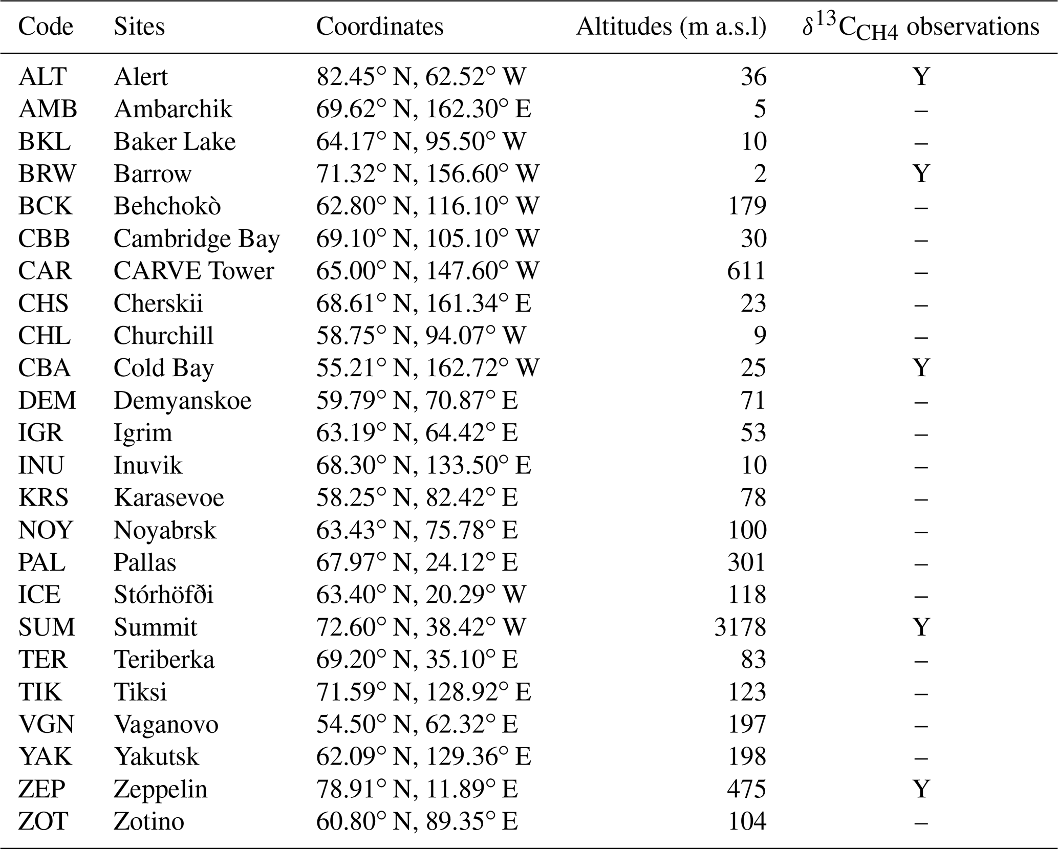
Table 1Description of the 24 sites measuring methane used in this study and included in our polar domain.
Following Thonat et al. (2017), who estimated the detectability of methane emissions at Arctic sites measuring total CH4, this paper aims at extending this approach to δ13CCH4 observations, even if they do not yet exist. After presenting the 24 existing monitoring sites in the northern high latitudes and the modelling framework (Sect. 2), we evaluate how well our model simulates δ13CCH4 at the five sites where it is already monitored (Sect. 3.1). Then, the atmospheric signals of the various northern high-latitude methane sources at these sites are estimated (Sect. 3.2) before determining their detectability based on instrumental constraints and on the uncertainties of the isotopic signatures (Sect. 3.3).
2.1 Measurements
Measurements of the isotopic ratio in atmospheric methane for 2012 come from five northern high-latitude surface sites (White et al., 2018). The locations of these sites are shown in Fig. 1, and their characteristics are given in Table 1. Most of them are considered to be sampling background air: Alert is located in northern Canada; Zeppelin (Ny-Ålesund) is on a mountaintop in the Svalbard archipelago; Cold Bay is in the Alaska Peninsula; and Summit is at the top of the Greenland Ice Sheet. The Barrow observatory (now known as Utqiaġvik), located in the North Slope of Alaska, is more affected by local wetland emissions. The NOAA Earth System Research Laboratory (NOAA ESRL) is responsible for the collection and analysis of the weekly flask samples. The isotopic composition is determined by INSTAAR (Institute of Arctic and Alpine Research) of the University of Colorado. All data are reported in conventional delta notation, in per mil (‰). The δ13CCH4 observations are given with a precision of better than 0.1 ‰ (White et al., 2018). All data without reported issues in collection or analyses are selected; outliers above 3σ of the variability at the station are discarded.
Other sites where atmospheric methane is measured are also included in this study. They do not provide δ13CCH4 observations, but we evaluate their potential in doing so. Their description is given in Table 1.
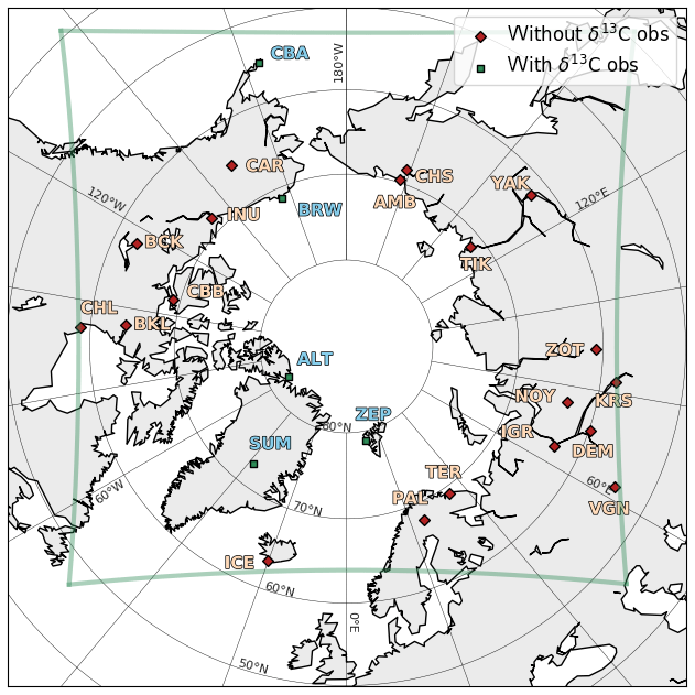
Figure 1Delimitation of the studied polar domain (green line), the location of the 24 measurement sites used in this study and measuring atmospheric methane. Five stations (blue squares) include flask measurements of δ13CCH4. The station name abbreviations are given in Table 1.
2.2 Model description
The Eulerian chemistry-transport model CHIMERE (Vautard et al., 2001; Menut et al., 2013) is used to simulate tropospheric 12CH4 and 13CH4 concentrations separately, with the isotope ratio being computed offline a posteriori. Following Thonat et al. (2017), the domain has a regular kilometric resolution of 35 km, which avoids numerical issues due to grid cells that are too small, close to the pole, and encountered in regular latitude–longitude grids. It covers all longitudes above 64∘ N but extend partially to 39∘ N, as illustrated in Fig. 1. The troposphere is divided into 29 vertical levels from the surface to 300 hPa (∼ 9000 m).
CHIMERE solves the advection–diffusion equation and is forced using meteorological fields from the ECMWF (European Centre for Medium Range Weather Forecasts, http://www.ecmwf.int/; last access: 18 September 2019) forecasts and reanalyses. Wind, temperature, water vapour, and other meteorological variables are given with a 3 h time resolution, at ∼ 0.5∘ spatial resolution, and 70 vertical levels in the troposphere. Initial and boundary concentrations of 12CH4 and 13CH4 come from a global simulation of the general circulation model LMDZ (Hourdin et al., 2006) for the year 2012. This global simulation used emission fluxes (including ORCHIDEE for wetland emissions, EDGARv4.2 for anthropogenic emissions other than biomass burning, and GFED4.1 for biomass burning emissions) that were adjusted in order to obtain a reasonable agreement at the global scale between the simulated isotopic signal and the flask measurements of the NOAA ESRL network (Dlugokencky et al., 1994). These global fields have a 3 h time resolution and spatial resolution. These meteorological and concentration fields are interpolated in time and space within the grid of the CHIMERE domain.
The model is run with various tracers, each one corresponding either to the 12CH4 or to the 13CH4 component of a methane source. Simulated 12CH4 and 13CH4 of all sources are then used in the calculation of δ13CCH4. This allows us to analyse the contribution of each source in δ13CCH4. Three pairs of tracers correspond to anthropogenic sources: emissions from oil and gas, emissions from solid fuels (coal), and other anthropogenic emissions (mostly from enteric fermentation and solid waste disposal). One pair of tracers corresponds to biomass burning. Two pairs correspond to geological sources: continental micro- and macroseepages; and marine seepages. Three pairs correspond to other natural sources: wetlands, freshwater systems, and emissions from the ESAS. Another pair of tracers corresponds to soil uptake and is considered as a negative surface source. Finally, one pair of tracers corresponds to the boundary conditions. No pair of tracers is implemented for the initial conditions: simulations in January are partly influenced by prescribed initial conditions from global fields during the spin-up period of 2–4 weeks (typical mixing time of air masses in the domain with the chosen model set-up spanning high northern-latitude regions), but this has little impact on our conclusions. No chemistry is included in the multi-tracers simulation, but another simulation including the reaction with OH is carried out in order to assess the contribution of this major sink. More details on the aforementioned emission categories are given below in Sect. 2.3.
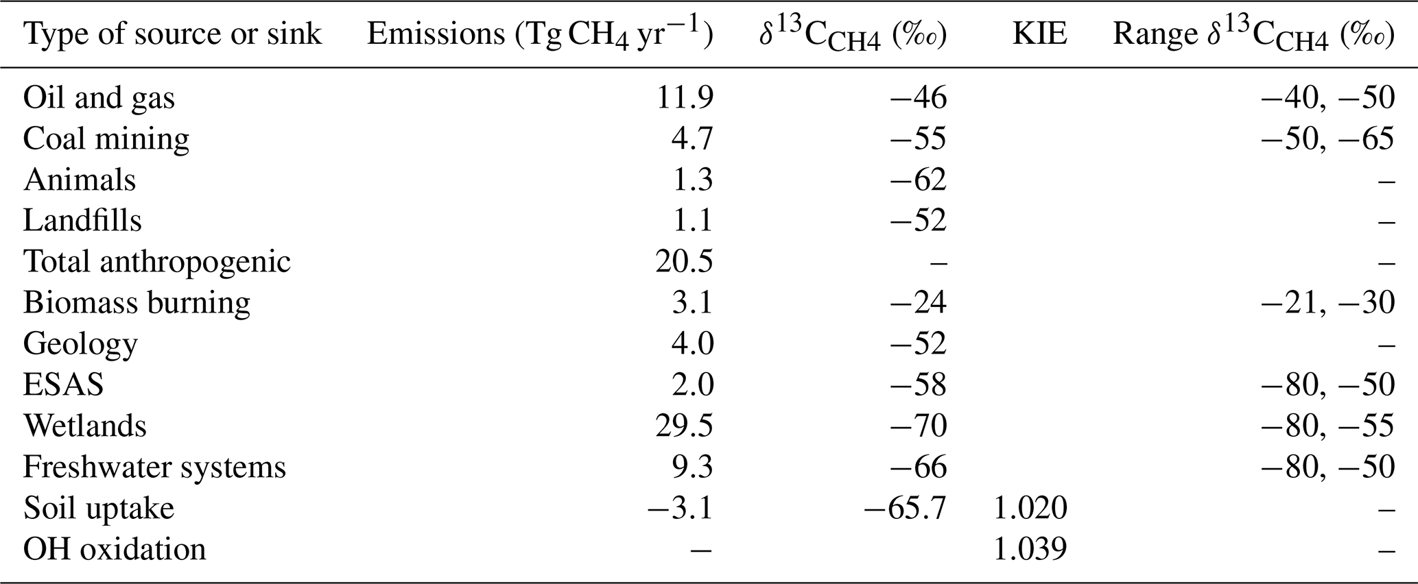
Table 2Methane emissions and isotopic signatures in the studied domain (see text within Sects. 2.3 and 2.4). Emission and sink fluxes used here are the same as in Thonat et al. (2017).
2.3 Input emission data
Surface emissions used as inputs in the model come from various inventories, models, and data-driven studies. The emissions used are the same as in Thonat et al. (2017), in which they are described and discussed in more detail; we provide a summary below and in Table 2.
All anthropogenic emissions are taken from the EDGARv4.2FT2010 yearly product (Olivier and Janssens-Maenhout, 2012). When possible, the 2010 data are updated using FAO (Food and Agriculture Organization, http://www.fao.org/faostat/en/\#data/, last access: 18 September 2019) and BP (http://www.bp.com/, last access: 18 September 2019) statistics (on enteric fermentation, and manure management, and on oil and gas production, fugitive from solid, respectively). For 2012, anthropogenic emissions amount to 20.5 Tg CH4 yr−1 in our domain, mostly from the fossil fuel industry. Biomass burning emissions come from the GFED4.1 (van der Werf et al., 2010; Giglio et al., 2013) daily product and represent 3.1 Tg CH4 yr−1 in our domain.
Wetland emissions are derived from the ORCHIDEE global vegetation model (Ringeval et al., 2010, 2011) on a monthly basis. Annual emissions from wetlands in our domain correspond to 29.5 Tg CH4 yr−1. A large uncertainty affects wetland emissions, which can vary widely depending on the chosen land vegetation model and wetland area dynamics (e.g. Bohn et al., 2015). Emissions from geological sources stem from the GLOGOS database (Etiope, 2015) and amount to 4.0 Tg CH4 yr−1 in our domain. ESAS emissions are prescribed to 2 Tg CH4 yr−1 in agreement with the estimate made by Thornton et al. (2016a) based on a ship measurement campaign and with the estimate made by Berchet et al. (2016) based on atmospheric observations at surface stations. The temporal and geographic variability of the ESAS emissions is based on the description by Shakhova et al. (2010), following the modelling framework of Berchet et al. (2016).
Following Thonat et al. (2017), we consider that 15 Tg CH4 yr−1 is emitted by all lakes and reservoirs located at latitudes above 50∘ N. The localization of these freshwater systems relies on the Global Lakes and Wetlands Database (GLWD) level 3 map (Lehner and Döll, 2004). Our inventory was built based on some simplifications: the emissions are uniformly distributed among lakes and reservoirs, no emissions occur when the lake is frozen, and emissions are constant otherwise. Freeze-up and ice-out dates are estimated based on surface temperature data from ECMWF ERA-Interim reanalyses. Freshwater emissions amount to 9.3 Tg CH4 yr−1 in our domain, which is consistent with recent pan-Arctic studies (e.g. Wik et al., 2016; Tan and Zhuang, 2015).
2.4 Source isotopic signatures
Source signatures are chosen constant in time and space in our modelling framework. Regional seasonal variations of microbial signatures are expected to be small (e.g. Sriskantharajah et al., 2012); some homogeneity can be assumed at the scale of our domain, which only comprises high northern latitudes, and possible heterogeneity is assumed to be smoothed out by the model 35 km horizontal resolution. Also, considering that most atmospheric sites are located far from large emission areas, the signals in the emissions are mixed by the atmospheric transport. Therefore, we have chosen to use only one value for each source but to test various scenarios with different isotopic signatures (see Sect. 3.2).
The Sherwood et al. (2017) data on fossil fuel emissions for countries within our domain show a wide range of measured isotopic signatures. For conventional gas and shale gas, data range between −76 ‰ and −24 ‰, with means for Russia (number of data, n=556), Canada (n=490), Norway (n=28), and the US (Alaska) (n=20), of −46 ‰, −51 ‰, −44 ‰, and −43 ‰, respectively. Heavier signatures (typically −40 ‰) are generally used for oil and gas related emissions in global studies (e.g. Houweling et al., 2006; Lassey et al., 2007) and also for Arctic studies (Warwick et al., 2016), but more depleted signatures have also been used for Russia (−50 ‰ in Levin et al., 1999). Given that Russia is by far the largest emitter of methane from natural gas production and distribution, we chose here a mean value of −46 ‰ for the whole domain, but test our results over a range spanning −40 ‰ to −50 ‰. As it is difficult to distinguish between methane associated with gas and oil exploitation, the same signature is used for both.
The range of isotopic values is also very large for emissions from coalfields: from −80 ‰ to −17 ‰ (Rice, 1993). In the Sherwood et al. (2017) database, isotopic signatures from coal exploitation are fewer than those from natural gas, with only one reference for Russia and 92 values reported for Canada, with a mean value of −55 ‰. Russia is again the top emitter in this category, but the paucity of the data prevents us from using the single value for the whole domain. Zazzeri et al. (2016) highlighted the dependence of the isotopic value on the coal rank and type of mining, although national and regional specificities remain. Basically, the higher the coal rank (i.e. the carbon content), the heavier the isotopic signature. The main Russian coal basins, the Kuznetsk and Kansk-Achinsk basins, located in southern Siberia, where low rank coal is extracted, are not part of our domain. The few major hotspots of emission associated with coal in our domain, according to EDGARv4.2FT2020, correspond to basins where hard coal is exploited, mainly bituminous coal (Podbaronova, 2010). According to the broad classification suggested by Zazzeri et al. (2016) for modellers, this means rather light isotopic signatures between −55 ‰ and −65 ‰. Consequently, we chose here a mean value of −55 ‰ for emissions associated with coal in our domain, which is lighter than the values usually used in global methane budgets (e.g. −37 ‰ in Bousquet et al., 2006, and Tyler et al., 2007; −35 ‰ in Monteil et al., 2011), but we test our results over the range of −50 ‰ to −65 ‰.
Other non-negligible anthropogenic sectors in our domain are enteric fermentation and waste disposal. For the former, the δ13C signature depends strongly on the ruminants' diets and on the species. Klevenhusen et al. (2010) found signatures from cows of −68 ‰ (C3 plants) or −57 ‰ (C4 plants), depending on the diet, in agreement with previous studies by Levin et al. (1999) and Bilek et al. (2001). Here, a value of −62 ‰ was used, as in other methane isotopic budgets (e.g. Tyler et al., 2007; Monteil et al., 2011). Methane emitted by organic waste is enriched as a result of methane oxidation after its production in the anoxic layer. Here, a value of −52 ‰ was used, in agreement with Chanton et al. (1999) (−58 ‰ to −49 ‰) and close to what was found by Bergamaschi et al. (1998) (−55 ‰). The emissions of those two sources are an order of magnitude lower than anthropogenic emissions from fossil fuel production; thus, their isotopic signature does not significantly impact the isotopic signal at observation sites.
Anthony et al. (2012) found natural seeps concentrated along the boundaries of permafrost thaw and retreating glaciers in Alaska and Greenland, with a wide range of isotopic signatures, originating from fossil and also younger methane. However, geological methane is mostly of thermogenic origin (Etiope, 2009), and this is also true for submarine seepage (e.g. Brunskill et al., 2011). In this region, geological manifestations occur through submarine seepages and microseepages with mean isotopic signatures of about −51.2 ‰ and −51.4 ‰ with uncertainty on the order of 7 ‰ and 2 ‰, respectively (Etiope et al., 2019). As a consequence, the isotopic signature used here for geological methane, both continental and submarine, is −52 ‰, following Etiope et al. (2019), associated with the range −50 ‰ to −55 ‰.
The values of isotopic signatures for biomass burning are found within a small range, despite their dependency on the fuel type (C3 vs. C4 plants) and combustion efficiency. For example, Chanton et al. (2000) reported values comprised between −30 ‰ and −21 ‰ for US forests. Yamada et al. (2006) estimated the global biomass burning δ13CCH4 at −24 ‰, while Whiticar and Schaefer (2007) suggested −25 ‰. Here, the value of −24 ‰ was used as a mean value, but signatures ranging from −30 ‰ to −21 ‰ have been tested (Table 3).
Table 3δ13CCH4 source signatures reported for wetlands at high northern latitudes.

Microbial methane from wetlands has a wide range of isotopic signatures, varying from −110 ‰ to −50 ‰ (Whiticar, 1999). Acetoclastic fermentation results in methane relatively less depleted in 13C (δ13CCH4 of −65 ‰ to −50 ‰), while CO2 reduction produces methane highly depleted in 13C (δ13CCH4 of −110 ‰ to −60 ‰) (Whiticar, 1999; McCalley et al., 2014). The partition between these two production pathways depends partly on the ecosystem type and season. The isotopic signature of the emitted methane also depends on other factors, such as the pathways of transport and oxidation (Chasar et al., 2000). Several studies on the isotopic signature of wetlands, focusing on high northern latitudes, are compiled in Table 3. All studies report values generally ranging between −75 ‰ and −60 ‰. Here again, the difficulty in dealing with these reported source signatures has to do with their representativity. Some observations are from chamber studies, which, by nature, focus on very local signals; others are given by ambient air samplings and can be representative of several hundred square kilometres, so possibly encompassing other source and sink determinants. The chamber studies present a wide variety of values for the same site. For example, Fisher et al. (2017) reported values at the Stordalen mire ranging from −112 ‰ to −48 ‰, and even in the same week, changes can be as large as 30 ‰. The signals can also vary significantly with the time of year and the kind of ecosystem (McCalley et al., 2014). For example, for three different peatland systems in Finland, Galand et al. (2010) report values that differed by 30 ‰. Consequently, values in Table 3 are mostly derived from ambient air samplings rather than chamber measurements, and we give means rather than the whole measured ranges. The value of −70 ‰ was used in our study and is close to the recommendation to modellers made by Fisher et al. (2017) () and France et al. (2016) for wetlands above 60∘ N. However we tested a wide range of signatures for wetland emissions between −80 ‰ and −50 ‰.
Most values labelled “Wetlands” in Table 3 encompass not only wetlands but also a mix of wetlands and other exposed freshwater systems. Shallow lakes, ponds, and pools, common in the Arctic, have not always been considered a distinct source (Bastviken et al., 2011). This is another limitation in estimating the global methane budget (Saunois et al., 2016). Signature estimates based on air sampling are representative of a wide area, where exposed freshwaters are undoubtedly present. Moreover, signature ranges reported specifically from Arctic lakes are not precise enough to distinguish between water body types and overlap those of wetlands (Wik, 2016). In the range of recent reported values (Walter et al., 2008; Brosius et al., 2012; Bouchard et al., 2015; Wik, 2016; Thompson et al., 2016), and close to the value used for Arctic wetlands, the value of −66 ‰ was used for the isotopic signature of freshwater system (here lakes and reservoirs) emissions in our domain. We also tested a wide range of signatures for freshwater emissions between −80 ‰ and −55 ‰.
Sources of methane in the ESAS are varied, and it is still a challenge to determine the origin of methane produced and emitted there (Ruppel, 2015). The shallow ESAS is underlain by formerly subaerial permafrost that has been flooded by sea level rise since the Pleistocene (Dmitrenko et al., 2011). Carbon can be released via the degradation of permafrost or decomposition of gas hydrates. Sapart et al. (2017) showed that sediments in ESAS have isotopic signatures ranging between the two main microbial methane formation pathways. In an earlier study, Cramer and Franke (2005) observed significantly heavier CH4 (δ13CCH4 ∼ −39.9 ‰) in the Laptev Sea near-surface sediments, which are attributed to a deep thermogenic source. A wider range, with much lighter CH4 was detected in the Laptev seawater column. Methane in the water is more enriched in 13C than in sediments, but the signature of methane emitted in the atmosphere is in the range of wetland emissions. Based on fewer data than Sapart et al. (2017), Overduin et al. (2015) reported more positive values, associated with strong 13C enrichment in the upper thawed permafrost layers. Oxidation in marine systems can be coupled to sulfate reduction as well in suboxic environments. This will not affect the atmospheric values directly but will shift the source signatures of the methane that is emitted from the surface to heavier values after having been diffusively advected from its sedimentary sites of production through the water column to the atmosphere. A mean signature of −58 ‰ (range −80 ‰ to −50 ‰) was used here for emissions from ESAS, in the range of the literature (Etiope et al., 2019).
2.5 Sinks: isotopic fractionation
The main sinks of methane in the troposphere are its oxidation by hydroxyl radicals (OH), which accounts for about 90 % of the total sinks (Saunois et al., 2016), its reaction with chlorine (Cl) in the marine boundary layer (about 3 %), and its uptake by soils (about 3 %, on a global scale; Kirshke et al., 2013).
Due to the difference in mass between the 12CH4 and 13CH4 isotopologues, chemical reactions in the atmosphere preferentially consume the lighter isotopologue, potentially causing significant fractionation. This is one of the reasons why the δ13C of methane in the atmosphere is not the same as that of the total source.
The chlorine sink is not included in our regional simulation. We have shown in Thonat et al. (2017) that this sink has a negligible impact of CH4 mixing ratio (below 1 ppb in our polar domain).
Methane uptake occurs in unsaturated oxic soils due to the presence of methanotrophic bacteria. This sink may be particularly important in high-latitude regions with wetlands. In our domain of simulation, its magnitude is equal to −3.1 Tg CH4 yr−1 (see Table 2).
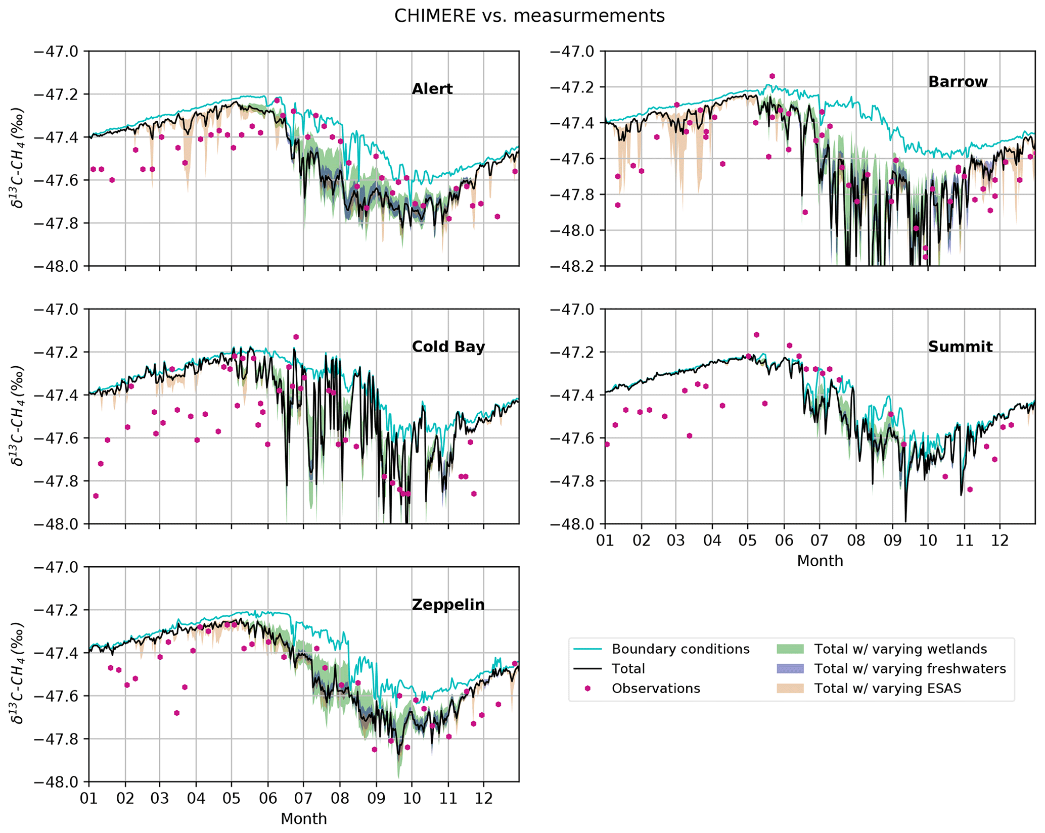
Figure 2Time series of simulated and observed δ13CCH4, at five sites, in 2012. The cyan line represents the contribution of the boundary conditions; and the black line represents the total simulated δ13CCH4 (boundary conditions + direct contribution of the sources located in the domain). The coloured shades represent total simulated δ13CCH4 with varying isotopic signatures (see Table 2) for wetlands (green), freshwater systems (blue), and ESAS (orange). The pink dots represent the flask observations. The hourly simulated values are averaged into daily values. (Note the different vertical scale for Barrow: the minimum for simulations at Barrow exceeds the chosen scale and reaches −49.3 ‰.)
Sinks can be characterized by their kinetic isotope effect (KIE). The ratio of the reaction rate coefficients (k) for two different isotopologues of the same molecule is klight∕kheavy. For the reaction with OH this value is 1.0039 (Saueressig et al., 2001). For the soil uptake, the KIE is 1.020, which is represented by a fixed δ13CCH4 source signature of −65.7 ‰ in our model set-up. Despite a high KIE, including the chlorine sink in the regional simulation will not change significantly our conclusions on the local source detectability.
Simulations of distinct tracers, each one corresponding to a different 12CH4 or 13CH4 source, are run with CHIMERE for the year 2012. Since isotopic signatures generally vary over a wide range for a given source (Sect. 2.3), we ran simulations using the mean value and the extreme values of the range given in Table 2 for oil and gas, coal, biomass burning, wetland, freshwater, and ESAS emissions.
3.1 Comparison between modelled and observed δ13CCH4
Most of the five sites, where weekly δ13CCH4 measurements are available, are remote from any emitting areas (Fig. 1) with the exception of Barrow, where significant methane enhancements from nearby wetlands can happen in summer (Sweeney et al., 2016). The boundary conditions are the dominant signal in our domain, especially in winter, both in terms of total methane mixing ratio (in ppb) and δ13CCH4 value (in ‰), as illustrated in Fig. 2. The boundary conditions represent methane coming from lower latitudes south of the polar domain (Fig. 1). However, they cannot be fully considered as a background level of methane given that (i) they may be due to emissions from the northern high latitudes that have left our domain and then re-entered it, and (ii) they may bring to the domain air masses that are particularly depleted or enriched in methane.
For most remote sites, the maximum δ13CCH4 is reached in May–June and ranges between −47.3 ‰ and −47.1 ‰ (Fig. 2). Then wetlands and freshwater systems start emitting 13C-depleted methane and the minimum is reached in September to early November, with values around −47.8 ‰. One exception is Cold Bay, where δ13CCH4 in January was much lower than other sites. In Barrow, the minimum reaches −48.2 ‰. The yearly mean is −47.6 ‰ at Barrow and −47.5 ‰ at the other sites. The seasonal amplitude is about 0.6 ‰. The variability of the measurements is higher in Barrow and Cold Bay compared to the three others, highlighting that these two sites are the most sensitive to northern high-latitude sources (mainly wetland emissions) at the synoptic scale.
The contribution of the boundary conditions to simulated δ13CCH4 is approximately between −47.2 ‰ and −47.6 ‰. The increment added by northern high-latitude sources lies between −0.1 ‰ and −0.2 ‰ in summer (June–October), except in Barrow where it is −0.4 ‰ and is close to zero in winter (November–May). Barrow is more sensitive to the regional sources (mainly wetland and freshwater emissions) compared to the four other sites (compare Fig. S4 to Figs. 4, S1, S10 and S18). On a yearly basis, our model overestimates δ13CCH4. The large overestimation in winter (∼ 0.2 ‰) is due to the boundary conditions that are too high in terms of total methane compared to continuous measurements (as shown in Thonat et al., 2017). Contributions of low-latitude fossil sources that are too large lead to δ13CCH4 values that are too high. Nevertheless, large spikes are simulated in winter at Barrow and Alert, some of which are attributed to ESAS emissions. Due to the low frequency of flask measurements, it is not possible to associate these simulated spikes to observed ones. Higher frequency measurements are needed to assess the reality of such spikes and their magnitudes and to allow discussion on both the magnitude of the source(s) and its/their isotopic signature(s). In summer, the model underestimates δ13CCH4 by less than 0.11 ‰ at all sites, which is in the range of the uncertainty of the measurements. However, the seasonality is only poorly captured by the model. The decrease in early summer comes too soon and so does the autumn minimum, as already noticed by Warwick et al. (2016). Thonat et al. (2017) demonstrated that this result is mostly emission driven: the seasonality of wetland emissions is not well reproduced by the various existing land surface models because wetland emissions derived from biogeochemical models occur too soon and cover too short a period during the year.
Despite their importance to assess the inter-annual variability and seasonality of δ13CCH4, the available flask measurements do not allow us to quantify the ability of the model to represent the synoptic variations. Continuous measurements of δ13CCH4, as well as δDCH4, would be necessary to evaluate the model in a more quantitative way. Even though further improvements will be necessary in the model, we assume in the following that the model performances associated with sensitivity tests using various isotopic signatures are sufficient for estimating the magnitude of the isotopic signals in δ13CCH4 originating from the various northern latitude sources.
3.2 Contributions of northern high-latitude sources in δ13CCH4 at northern latitude sites
In terms of total methane, our domain is dominated by anthropogenic sources in winter and by wetland emissions in summer. ESAS and geological sources can also have a relatively significant impact in winter in some areas, while freshwater systems are an important contributor to atmospheric methane in summer (Thonat et al., 2017). The spatial distribution of the source contribution to the δ13CCH4 value depends not only on the magnitude of the emission but also on the difference between the isotopic signature of the source and of the boundary conditions. The difference between total δ13CCH4 and the contribution of the boundary conditions (Fig. 2, black and cyan lines, respectively) represents the sum of the direct contribution from the various northern latitude sources at the measurement locations. The combination of the various signals due to northern latitude sources depends on the station, as shown in Fig. 2.
These five sites do not form a large enough sample to be representative of all northern latitude sites. Therefore, Fig. 3 shows the winter and summer means of the simulated direct contributions of the various sources to the δ13CCH4 value at the 24 sites of Fig. 1. For each site, the seasonal mean contribution of each source is plotted along a cumulative dotted line. The rightmost black point of each line represents the total contribution of all northern latitude sources, i.e. the difference between simulated total δ13CCH4 and δ13CCH4 from the boundary conditions alone. The frequency distribution of the contribution from all the Arctic sources to the signal is overplotted with an arbitrary unit, showing the range of isotopic signals covered over the season. For example, if we consider Tiksi (TIK) in winter, the direct contribution of all Arctic sources is −0.09 ‰ on average over the season. However, the frequency distribution shows that the isotopic contribution at Tiksi is mainly between 0 and −0.2 ‰ but can reach lower values up to −0.25 ‰.
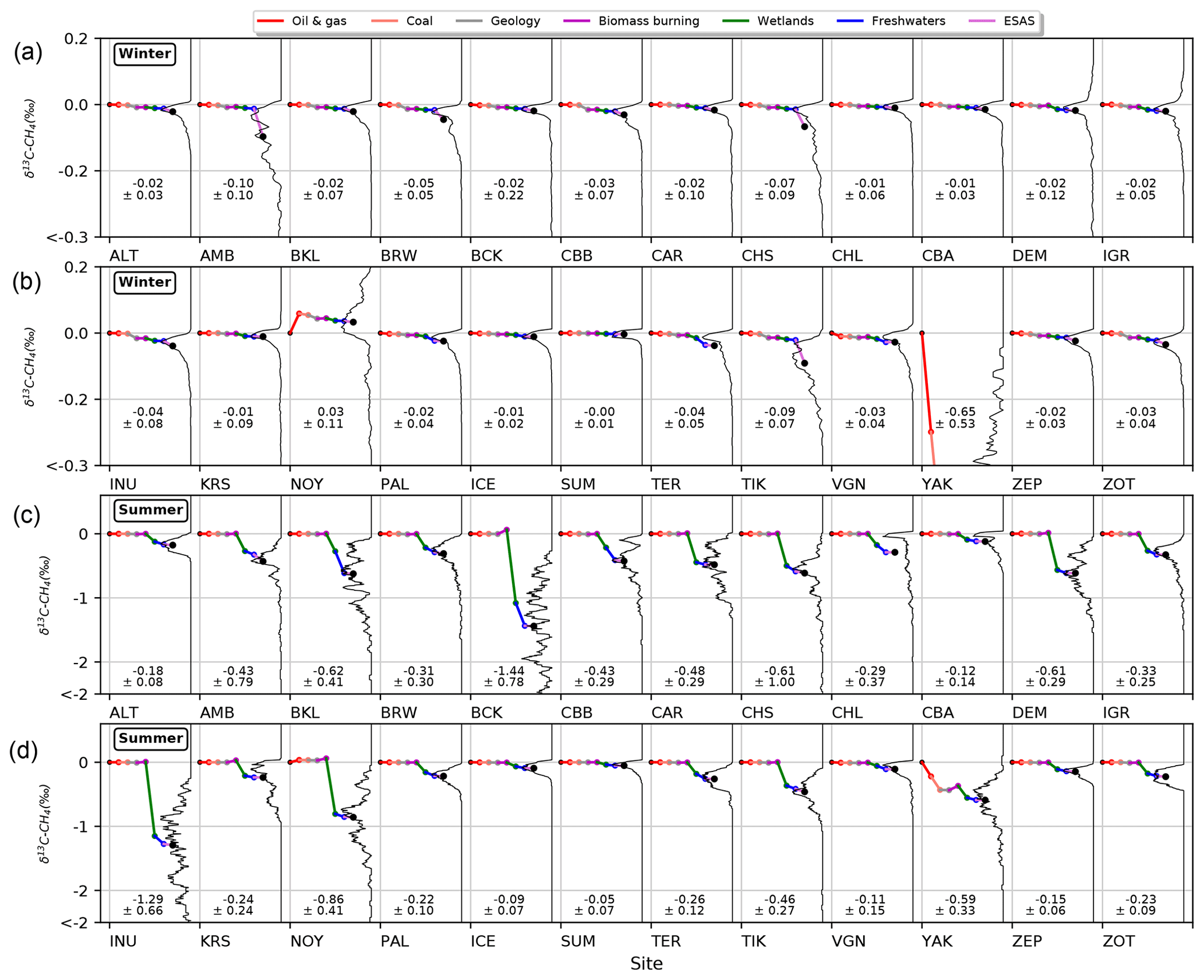
Figure 3Winter (a, b) and summer (c, d) means of the direct contributions of the various northern high-latitude sources to the δ13CCH4 value (in ‰) simulated by CHIMERE at 24 sites in 2012. The frequency distribution of daily signatures at each site is overplotted with an arbitrary unit on the x axis, showing the simulated spread of the signal over the season. For each station and season, the number indicates the mean δ13CCH4 value (in ‰) associated with its 1σ value. See Sect. 3.2 further details.
On average, the contributions of northern high-latitude sources to the isotope ratio are very low in winter at all sites, between −0.65 ‰ and +0.03 ‰. The isotope ratio signal is low in winter because the largest contribution of Arctic sources to atmospheric methane in this season is due to oil and gas emissions, whose signature (−46 ‰) is very close to that of boundary conditions. One exception is YAK (see Table 1 for the definition of site abbreviations here and hereafter), where the mean winter contribution to δ13CCH4 is −0.63 ‰. This is due to large simulated mixing ratios of methane from nearby coal emissions. The daily isotope ratio signal shift due to Arctic contributions there can reach −1.75 ‰. Geological emissions have a signature close to oil and gas in our modelling framework and do not show up in the simulated signal. On the contrary, ESAS emissions have an impact on δ13CCH4 at some sites at the synoptic scale: the maximum δ13CCH4 northern high-latitude contribution at AMB and CHS in winter is ∼ −0.5 ‰ and ∼ −0.4 ‰ at TIK, which are close to the shores of ESAS. NOY is the only site with a positive mean contribution to δ13CCH4 in winter. Large enhancements of 12CH4 from oil and gas, which in NOY regularly exceeds 100 ppb in winter, succeed in making a significant difference with the δ13CCH4 value of the boundary conditions. Apart from NOY, the northern high-latitude contribution to δ13CCH4 is very rarely positive among the sites and stays low when it is positive (maximum is 0.13 ‰ at DEM).
Compared to winter, higher contributions of northern high-latitude sources to the δ13CCH4 values are found in summer at most stations because of the large magnitude of natural emissions, especially from wetlands. Wetland emissions contribute to more than two-thirds of the signal at all sites, except at BKL and CBB where the contribution of freshwater systems is also important, and at YAK (again due to coal emissions). Wetlands keep the isotope ratio quite low, with two sites having a mean δ13CCH4 contribution more negative than −1.0 ‰ (BCK and INU). Values below −2.0 ‰ are even reached on a daily basis at 15 sites; it is frequent at BCK for example, where the influence of wetlands and freshwater systems are combined. On top of wetland and freshwater influences, ESAS explains more than 10 % of the signal at TIK and AMB.

Figure 4Time series of δ13CCH4 contributions of each source (in ‰), simulated by CHIMERE, in Zeppelin in 2012. The coloured shades represent the range of δ13CCH4 values when varying isotopic signatures (see Table 2). (Note the different scales.)
Figure 3 reveals what can be expected on a seasonal basis at the different sites, but it does not show how the various source contributions combine all along the year and how different source signatures can affect the total δ13CCH4 signal. Figures 4 and S1–S23 show the time series of the direct contribution of each source and sink to the total δ13CCH4 at the 24 northern latitude stations. A focus is put on Zeppelin station in Fig. 4 because a new Aerodyne instrument has been installed there during Summer 2018 in order to continuously measure δ13CCH4 for at least 1 year. Figure 4 illustrates the magnitude and timing of the maximum signal of each source during the year, the potential compensation between sources, and the seasonality of the various contributions.
Zeppelin is a typical example of a remote site. The δ13CCH4 values from anthropogenic emissions are very small (< 0.02 ‰, except for some particular events which concern the lightest isotopic signatures) because the source areas are far from the station and tend to be cancelled out because the signals from oil and gas, and from coal have approximately the same magnitude but opposite signs. The signal from geological sources remains negligible being 1 order of magnitude lower than anthropogenic sources. Only wetland emissions succeed to tear the signal away from the value of the boundary conditions, from June to October, with synoptic changes up to −0.2 ‰. Freshwater systems intensify the signal by 0.02 ‰ on average in summer, with maxima around 0.05 ‰ on a synoptic basis. These contributions are diminished by biomass burning (∼ +0.01 ‰) and also by the fractionating effects of the two major sinks (∼ +0.01 ‰). The simulated δ13CCH4 signal at the site is the result of these competing signals. Varying the isotopic signatures of natural sources does not change the conclusions with wetland, freshwater, and ESAS synoptic events reaching at maximum −0.3 ‰, −0.1 ‰, and −0.15 ‰, respectively . Therefore, in the case of a remote station such as ZEP, signals of individual sources remain below 0.3 ‰ at the synoptic scale, and partial compensation between sources determines the total δ13CCH4 anomaly.

Figure 5Number of days in 2012 when simulated daily direct contributions of northern high-latitude sources to the δ13CCH4 value are above given thresholds, for each of the 24 stations of Fig. 1. The numbers on the top left of each wind rose correspond to the threshold values. The coloured shades indicate the dominant northern high-latitude source in terms of δ13CCH4 contribution.
Analysing other stations (Figs. S1–S23) reveals that synoptic events larger than 2 ‰ due to summer wetland emissions could happen at AMB, BCK, CHS, DEM, IGR, INU, NOY, and TIK. For freshwater emissions, events larger than 0.5 ‰ are simulated at AMB, BKL, BRW, BCK, CBB, CHL and INU. For ESAS, varying the isotopic signature induces synoptic events larger than 0.3 ‰ at some sites (AMB, BRW, CHS, and TIK). When varying the isotopic signature of anthropogenic emissions, DEM, IGR, KRS, NOY, and VGN show synoptic events due to oil and gas that are larger than 0.15 ‰, and only YAK shows synoptic events due to fugitive emissions larger than 1 ‰; these events occur mainly in winter. Biomass burning synoptic events are the largest at BCK, DEM, KRS, NOY, and YAK with events larger than 0.2 ‰.
The influence of the sinks on synoptic variations remains smaller than 0.05 ‰ at most sites. Note that the sink constituted by the reaction with Cl radicals in the marine boundary layer is not taken into account here, given its very small impact on CH4-mixing ratios in our domain (less than 1 ppb, Thonat et al., 2017), although it is highly fractionating. As aforementioned, including this sink in the regional simulation will not change significantly our conclusions on the local source detectability.
3.3 Detectability of northern high-latitude sources using isotopic measurements
The magnitude of δ13CCH4 signals to be expected at present and potential measurement sites and the contributions of individual sources to these signals do not lead directly to quantifying the detectability of individual sources, as the latter also depends on the performances of the measuring instrument. Here we focus on a detectability definition taken from a regional inversion point of view: regional inversion systems analyse daily signals and optimize sources depending on synoptic deviations of the observed signals compared to the simulated ones. Therefore, a measuring instrument is considered to provide useful information to the inversion only if the synoptic variability of the atmospheric signal can be detected. To that end, we compute detectability capability in Fig. 5 and Table 4 as follows: (1) we compute the standard deviation over a 5 d running window of the simulated total isotopic signal; (2) for a set of instrument precision threshold (from 0.2 ‰ to 0.01 ‰, see Fig. 5 and Table 4), if the running standard deviation is higher than the corresponding threshold, the source with the higher running standard deviation for the same 5 d window is considered detected for that one day; (3) for each threshold, we count the number of days over the year that each source is detected. Although the total atmospheric signal integrates contributions from different sources with different isotopic signatures, we keep only the major source contributing to the signal as a 1st-order signal.
Table 4Minimum detectability threshold (in ‰) of high northern-latitude sources at all observation sites in 2012 considering the mean values of isotopic signature in Table 2. See Sect. 3.3 for the definition of the detectability threshold.
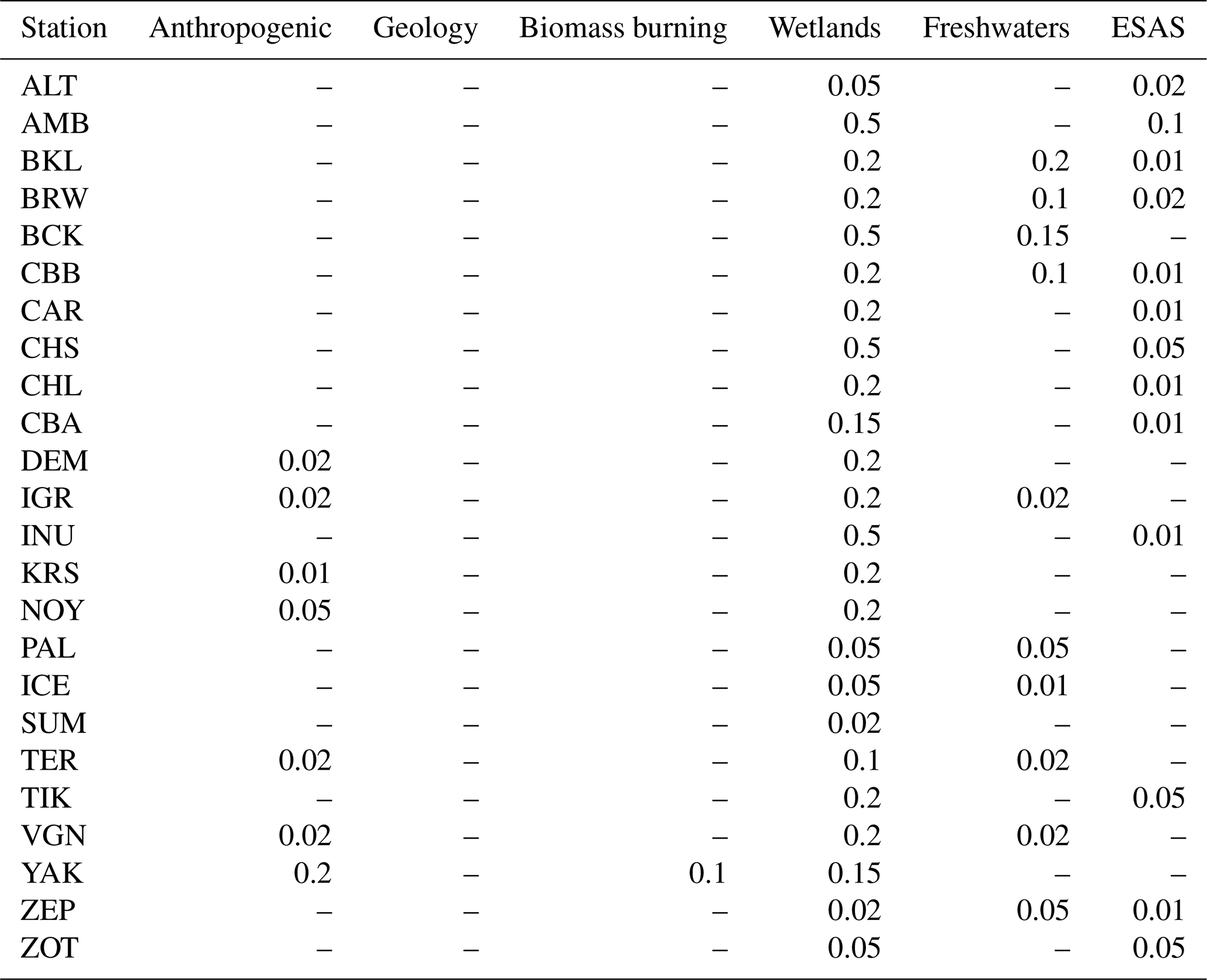
The range of instrument precision threshold was chosen according to present isotopic instrument systems. The flask measurements used in Sect. 3.1 (Table 1, Figs. 1 and 2) have an uncertainty of about 0.1 ‰. They were obtained using GC–IRMS (gas chromatography–isotope ratio mass spectrometry; White et al., 2018). Using continuous-flow isotope ratio mass spectrometry, Fisher et al. (2006) reached a precision of 0.05 ‰. Laser-based instruments, using cavity ring-down spectrometry or direct absorption spectrometry (Nelson et al., 2004), have been developed since 10 years for CO2 isotopes (McManus et al., 2010) and, more recently for methane (Santoni et al., 2012). The Aerodyne QCL instrument has proven to be capable of high-frequency (≥ 1 Hz) measurements of 12CH4 and 13CH4 isotopes of CH4 with in situ 1 s rms precision of 1.5 ‰ and an Allan minimum precision of 0.2 ‰ at 100 s (Santoni et al., 2012), recently improved to 0.1 ‰ through laser stability improvements. Such a small value (0.1 ‰) reaches the precisions reported for GC–IRMS (0.1 ‰). However, Aerodyne instruments face a strong drift that imposes a strict calibration protocol (every 2 h in the most recent set-ups), which dramatically reduces the daily number of available observations to typically a few tens. Depending on our capability to deploy stable and well-calibrated instruments in very remote high-latitude sites, state-of-the art isotopic instruments may provide from a few to hundreds of independent data points per day thus potentially improving the instrument precision of daily averaged observations to 0.01 ‰.
Detectability thresholds at the 24 sites of Table 1 are summarized in Table 4 and Fig. 5 when considering the mean values of the isotopic signatures of Table 2. Results for a 0.5 ‰ threshold are not shown in Fig. 5 because only the YAK station can detect sources (only the oil and gas sector) at this level of instrument precision. At ZEP, with an uncertainty higher than or equal to 0.1 ‰, no source is detected. Currently, daily flask measurements are operated at ZEP with an uncertainty of 0.05 ‰ but contamination problems occur. If such contaminations are avoided so that the measurement uncertainty reaches 0.05 ‰, some wetland events may be detected for about 10 individual days over the year. From 0.05 ‰ of measurement uncertainty, the number of events is larger and other sources (freshwater and ESAS emissions) might be detected. At only 0.01 ‰, there were about 20 d of possible detection for ESAS, a few days for freshwaters, and none for anthropogenic emissions. Looking at results for all stations, wetland emissions are the most easily detected with more than 50 d for a measurement uncertainty above 0.1 ‰ for most sites (with the exception of ALT, BKL, CHL, ICE, PAL, SUM, SUM, ZEP, and ZOT); the best scores of detection, with more than 150 d, are achieved at BCK, INU, DEM, and NOY. Freshwater emissions are easiest to detect at BKL and CBB with 100 d and 50 d above 0.1 ‰ respectively. Anthropogenic emissions are easily detected at YAK due to its close location to coal extraction sites. With a 0.05 ‰ uncertainty, most of the stations offer opportunities to detect regional sources, except remote stations and/or stations close to the boundaries of our domain (ALT, CHL, ICE, SUM, and ZEP). For ESAS emissions, the minimum detection ranges between 0.02 ‰ and 0.1 ‰ depending on stations. ESAS emissions are best detected at AMB, CHS, and TIK with more than 50 d above 0.05 ‰. A few other sites offer detectability if uncertainties are lower than 0.02 ‰ (ALT, BRW, BKL, CBB, CHL, INU, and ZOT). As already noticed, the effect of anthropogenic emissions dominates at YAK with about 100 d above 0.2 ‰ uncertainty. Other sites located in Russia are able to detect anthropogenic emissions with more than 50 d of events above 0.02 ‰ (DEM, IGR, NOY, and VGN). Excluding YAK, the minimum detection of anthropogenic emissions ranges between < 0.01 ‰ and 0.05 ‰ depending on stations. For the year 2012, YAK and KRS detected some biomass burning events with an uncertainty lower than 0.2 ‰ and 0.1 ‰ , respectively. Geological sources are detected at ZOT when the uncertainty is lower than 0.01 ‰.
Although no continuous δ13CCH4 observed time series are available yet, inverse modellers have been considering δ13CCH4 observations as a promising way to distinguish methane sources (e.g. Hein et al., 1997). The assimilation of δ13CCH4 flask data into 3-D chemistry-transport global models has shown small changes in the balance of sources, involving mostly biomass burning at the global scale (Bousquet et al., 2006, p. 7 in their Supplement). This modest impact was explained by the scarcity of δ13CCH4 observations (only 13 flask stations in Bousquet et al., 2006) and the uncertainties on isotopic signatures. Since then the former has slightly improved at the global scale (20 flask sites reported in the World Data Center for Greenhouse Gases database at present; http://gaw.kishou.go.jp/, last access: 18 September 2019) and continuous measurements are expected (e.g. Thornton et al., 2016b), but the latter is still an issue because it is necessary to obtain precise isotopic signatures at the regional scale for the various processes emitting methane. Three-dimensional atmospheric forward modelling has also been used to interpret methane changes over the past decades through scenarios of methane emissions, methane sinks, and isotopic signatures (Monteil et al., 2011; Warwick et al., 2016), demonstrating the added value of the global monitoring of methane isotopes, although the above limitations are still present. Taking into account these limitations, the most recent inverse studies integrating δ13CCH4 data have only used simple box models and, therefore, have assimilated hemispheric or global mean time series of 13C observations (e.g. Schaefer et al., 2016; Turner et al., 2017; Schwietzke et al., 2016). Such studies use strong simplifications in their set-up and can obviously only address hemispheric to global-scale emissions and trends.
Our work aims at preparing 3-D inversions assimilating future continuous δ13CCH4 time series to address the reduction of uncertainties on methane emissions at the regional scale. The northern high latitudes have been chosen to make this first analysis because it is a climate-sensitive region (with potentially larger methane sources than those of today in the context of a changing climate), and because the mix of methane sources is less complicated than in the tropics. Even in this apparently favourable context, the situation of the detectability of methane sources using δ13CCH4 observations is found challenging for at least three reasons. First, as already noted in Thonat et al. (2017), most of the methane signals received at northern latitude stations at the synoptic to seasonal scales come from lower latitudes, thus limiting the expected signal-to-noise ratio of the northern high-latitude sources. Second, the analysis presented in Sect. 3 reveals that, if isotopic signals from wetland emissions would be detectable at most existing sites with reasonable measurement uncertainties on a daily basis (∼ 0.15 ‰), detecting other sources would require more challenging measurement uncertainties: typically less than 0.05 ‰ for freshwaters, ESAS, and anthropogenic emissions (except at YAK); and less than 0.02 ‰ for other sources. Such ambitious values require solving or at least monitoring precisely the present drifts of existing instruments and stress the importance of having a precise scale for regular calibration. Third, the vision per source developed here is optimistic as total isotopic signals received at stations may cancel each other out for some events, thus reducing the number of useful events constraining individual sources. It should be noted that we provide here a 1st-order contribution in the signal, while air is mixed in the atmosphere and the total signal integrates contributions from different sources. As a result, the threshold and the main contributing source both depend on the isotopic signatures assigned to the different sources (Figs. S24–S27). For example, if the heaviest (−50 ‰) isotopic signature from Table 2 is assigned to wetland emissions, then this source is hardly detected for measurement uncertainties higher than 0.05 ‰, while the lightest signature allows a detection for a 0.2 ‰ measurement uncertainty at more than half the sites. Similarly, freshwater or ESAS emissions are considered detectable with a measurement uncertainty of 0.2 ‰ at Russian sites when applying the lightest isotopic signatures. This study has been carried out only for the year 2012 as a test case. However, not all emissions have a high interannual variability, as does biomass burning. As a result, our findings should be valid for the other sources for most of the years over some future decades.
The next steps of this work involve (i) the analysis of more than 1 year of continuous measurements of δ13CCH4 at ZEP, (ii) the refinement of isotopic signatures of the various emissions at the regional scale, (iii) the implementation of δ13CCH4 in inversion schemes in order to estimate the potential (if only pseudo-continuous data were available) or the actual impact of δ13CCH4 in improving the estimation of regional methane emissions by 3-D atmospheric inversions, and (iv) assessing the potential of δDCH4 in both global and regional modelling framework.
The data for δ13CCH4 observations were downloaded from the World Data Centre for Greenhouse Gases (WDCGG) at https://gaw.kishou.go.jp (last access: 18 September 2019; WDCGG, 2019). Datasets for the input emissions were downloaded from the EDGAR and GFED databases. The modelling output files are available upon request from the corresponding author.
The supplement related to this article is available online at: https://doi.org/10.5194/acp-19-12141-2019-supplement.
TT, MS, PB, and IP designed the study. BFT and PMC brought expertise on observation availability and instrument performance. TT performed the regional simulations. TH performed the global simulations used as boundary conditions. AB and TT produced the figures. TT and MS prepared the paper. All co-authors contributed to the analysis, the design of the figures, and the text.
The authors declare that they have no conflict of interest.
The authors acknowledge the principal investigators, Bruce Vaughn, James White, and Sylvia Michel, of the five observation sites measuring 13CH4 in the Arctic regions, whose data were used in this study, and we thank them for maintaining methane measurements at high latitudes and sharing their data through the World Data Centre for Greenhouse Gases (WDCGG). The study extensively relies on the meteorological data provided by the ECMWF. Calculations were performed using the computing resources of LSCE, maintained by François Marabelle and the LSCE IT team. The authors warmly acknowledge the two anonymous referees, whose help improved the paper and the conclusions of this study.
This research has been supported by the Swedish Research Council VR through a French-Swedish project named IZOMET (Distinguishing Arctic CH4 sources to the atmosphere using inverse analysis of high-frequency CH4, 13CH4 and CH3D measurements) (grant No. VR 2014-6584)
This paper was edited by Patrick Jöckel and reviewed by two anonymous referees.
Anthony, K. M. W., Anthony, P., Grosse, G., and Chanton, J. P.: Geologic methane seeps along boundaries of Arctic permafrost thaw and melting glaciers, Nat. Geosci., 5, 419–426, https://doi.org/10.1038/ngeo1480, 2012.
Bastviken, D., Tranvik, L. J., Downing, J. A., Crill, P. M., and Enrich-Prast, A.: Freshwater methane emissions offset the continental carbon sink, Science, 331, 50 pp., https://doi.org/10.1126/science.1196808, 2011.
Berchet, A., Pison, I., Chevallier, F., Paris, J.-D., Bousquet, P., Bonne, J.-L., Arshinov, M. Y., Belan, B. D., Cressot, C., Davydov, D. K., Dlugokencky, E. J., Fofonov, A. V., Galanin, A., Lavrič, J., Machida, T., Parker, R., Sasakawa, M., Spahni, R., Stocker, B. D., and Winderlich, J.: Natural and anthropogenic methane fluxes in Eurasia: a mesoscale quantification by generalized atmospheric inversion, Biogeosciences, 12, 5393–5414, https://doi.org/10.5194/bg-12-5393-2015, 2015.
Berchet, A., Bousquet, P., Pison, I., Locatelli, R., Chevallier, F., Paris, J.-D., Dlugokencky, E. J., Laurila, T., Hatakka, J., Viisanen, Y., Worthy, D. E. J., Nisbet, E., Fisher, R., France, J., Lowry, D., Ivakhov, V., and Hermansen, O.: Atmospheric constraints on the methane emissions from the East Siberian Shelf, Atmos. Chem. Phys., 16, 4147–4157, https://doi.org/10.5194/acp-16-4147-2016, 2016.
Bergamaschi, P., Lubina, C., Königstedt, R., Fischer, H., Veltkamp, A. C., and Zwaagstra, O.: Stable isotopic signatures (δ13C, δD) of methane from European landfill sites, J. Geophys. Res., 103, 8251–8265, https://doi.org/10.1029/98JD00105, 1998.
Bernard, S.: Evolution temporelle du méthane et du protoxyde d'azote dans l'atmosphère: contrainte par l'analyse de leurs isotopes stables dans le névé et la glace polaires, PhD dissertation, Univ. Grenoble 1, available at: https://tel.archives-ouvertes.fr/tel-00701325 (last access: 18 September 2019), 2004.
Bilek, R. S., Tyler, S. C., Kurihara, M., and Yagi, K.: Investigation of cattle methane production and emission over a 24-hour period using measurements of δ13C and δD of emitted CH4 and rumen water, J. Geophys. Res., 106, 15405–15413, https://doi.org/10.1029/2001JD900177, 2001.
Bohn, T. J., Melton, J. R., Ito, A., Kleinen, T., Spahni, R., Stocker, B. D., Zhang, B., Zhu, X., Schroeder, R., Glagolev, M. V., Maksyutov, S., Brovkin, V., Chen, G., Denisov, S. N., Eliseev, A. V., Gallego-Sala, A., McDonald, K. C., Rawlins, M. A., Riley, W. J., Subin, Z. M., Tian, H., Zhuang, Q., and Kaplan, J. O.: WETCHIMP-WSL: intercomparison of wetland methane emissions models over West Siberia, Biogeosciences, 12, 3321–3349, https://doi.org/10.5194/bg-12-3321-2015, 2015.
Bouchard, F., Laurion, I., Prėskienis, V., Fortier, D., Xu, X., and Whiticar, M. J.: Modern to millennium-old greenhouse gases emitted from ponds and lakes of the Eastern Canadian Arctic (Bylot Island, Nunavut), Biogeosciences, 12, 7279–7298, https://doi.org/10.5194/bg-12-7279-2015, 2015.
Bousquet, P., Ciais, P., Miller, J., Dlugokencky, E., Hauglustaine, D., Prigent, C., Van der Werf, G., Peylin, P., Brunke, E.-G., and Carouge, C.: Contribution of anthropogenic and natural sources to atmospheric methane variability, Nature, 443, 439–443, 2006.
Bousquet, P., Pierangelo, C., Bacour, C., Marshall, J., Peylin, P., Ayar, P. V., Ehret, G., Bréon, F.-M., Chevallier, F., Crevoisier, C., Gibert, F., Rairoux, P., Kiemle, C., Armante, R., Bès, C., Cassé, V., Chinaud, J., Chomette, O., Delahaye, T., Edouart, D., Estève, F., Fix, A., Friker, A., Klonecki, A., Wirth, M., alpers, M., and Millet, B.: Error budget of the MEthane Remote LIdar missioN and its impact on the uncertainties of the global methane budget, J. Geophys. Res.-Atmos., 123, 11766–11785, https://doi.org/10.1029/2018JD028907, 2018.
Brosius, L. S., Walter Anthony, K. M., Grosse, G., Chanton, J. P., Farquharson, L. M., Overduin, P. P., and Meyer, H.: Using the deuterium isotope composition of permafrost meltwater to constrain thermokarst lake contributions to atmospheric CH4 during the last deglaciation, J. Geophys. Res., 117, G01022, https://doi.org/10.1029/2011JG001810, 2012.
Brunskill, G. J., Burns, K. A., and Zagorskis, I.: Natural flux of greenhouse methane from the Timor Sea to the atmosphere, J. Geophys. Res., 116, G02024, https://doi.org/10.1029/2010JG001444, 2011.
Cain, M., Warwick, N. J., Fisher, R. E., Lowry, D., Lanoisellé, M., Nisbet, E. G., France, J., Pitt, J., O'Shea, S., Bower, K. N., Allen, G., Illingworth, S., Manning, A. J., Bauguitte, S., Pisso, I., and Pyle, J. A.: A cautionary tale: A study of a methane enhancement over the North Sea, J. Geophys. Res. Atmos., 122, 7630–7645, https://doi.org/10.1002/2017JD026626, 2017.
Chanton, J. P., Rutkowski, C. M., and Mosher, B.: Quantifying methane oxidation from landfills using stable isotope analysis of downwind plumes, Environ. Sci. Tech., 33, 3755–3760, https://doi.org/10.1021/es9904033, 1999.
Chanton, J. P., Rutkowski, C. M., Schwartz, C. C., Ward, D. E., and Boring, L.: Factors influencing the stable carbon isotopic signature of methane from combustion and biomass burning, J. Geophys. Res., 105, 1867–1877, https://doi.org/10.1029/1999JD900909, 2000.
Chasar, L. S., Chanton, J. P., Glaser, P. H., and Siegel, D. I.: Methane concentration and stable isotope distribution as evidence of rhizospheric processes: comparison of a fen and bog in the glacial lake Agassiz peatland complex, Ann. Bot., 86, 655–663, https://doi.org/10.1006/anbo.2000.1172, 2000.
Ciais, P., Sabine, C., Bala, G., Bopp, L., Brovkin, V., Canadell, J., Chhabra, A., DeFries, R., Galloway, J., Heimann, M., Jones, C., Le Quéré, C., Myneni, R. B., Piao, S., and Thornton, P.: Carbon and Other Biogeochemical Cycles, in: Climate Change 2013: The Physical Science Basis. Contribution of Working Group I to the Fifth Assessment Report of the Intergovernmental Panel on Climate Change, edited by: Stocker, T. F., Qin, D., Plattner, G.-K., Tignor, M., Allen, S. K., Boschung, J., Nauels, A., Xia, Y., Bex, V., and Midgley, P. M., Cambridge University Press, Cambridge, United Kingdom and New York, NY, USA, 2013.
Craig, H.: Isotopic standards for carbon and oxygen and correction factors for mass spectrometric analysis of carbon dioxide, Geochim. Cosmochim. Ac., 12, 133–149, 1957.
Cramer, B. and Franke, D.: Indications for an active petroleum system in the Laptev Sea, NE Siberia, J. Petrol. Geol., 28, 369–384, https://doi.org/10.1111/j.1747-5457.2005.tb00088.x, 2005.
Dlugokencky, E. J., Steele, L. P., Lang, P. M., and Masarie, K. A.: The growth rate and distribution of atmospheric methane, J. Geophys. Res., 99, 17021–17043, https://doi.org/10.1029/94JD01245, 1994.
Dlugokencky, E. J., Nisbet, E. G., Fisher, R., and Lowry, D.: Global atmospheric methane: budget, changes and dangers, Philos. T. Roy. Soc. A, 369, 2058–2072, https://doi.org/10.1098/rsta.2010.0341, 2011.
Dmitrenko, I. A., Kirillov, S. A., Tremblay, L. B., Kassens, H., Anisimov, O. A., Lavrov, S. A., Razumov, S. O., and Grigoriev, M. N.: Recent changes in shelf hydrography in the Siberian Arctic: Potential for subsea permafrost instability, J. Geophys. Res., 116, C10027, https://doi.org/10.1029/2011JC007218, 2011.
Etiope, G.: Natural emissions of geological methane in Europe, Atmos. Environ., 43, 1430–1443, https://doi.org/10.1016/j.atmosenv.2008.03.014, 2009
Etiope, G.: Natural gas seepage, The Earth's hydrocarbon degassing, Springer International Publishing, Switzerland, https://doi.org/10.1007/978-3-319-14601-0, 2015.
Etiope, G., Ciotoli, G., Schwietzke, S., and Schoell, M.: Gridded maps of geological methane emissions and their isotopic signature, Earth Syst. Sci. Data, 11, 1–22, https://doi.org/10.5194/essd-11-1-2019, 2019.
Etminan, M., Myhre, G., Highwood, E. J., and Shine, K. P. : Radiative forcing of carbon dioxide, methane, and nitrous oxide: A significant revision of the methane radiative forcing, Geophys. Res. Lett., 43, 12614–12623, https://doi.org/10.1002/2016GL071930, 2016.
Fisher, R. E., Sriskantharajah, S., Lowry, D., Lanoisellé, M., Fowler, C. M. R., James, R. H., Hermansen, O., Lund Myhre, C., Stohl, A., Greinert, J., Nisbet‐Jones, P. B. R., Mienert, J., and Nisbet, E. G.: Arctic methane sources: Isotopic evidence for atmospheric inputs, Geophys. Res. Lett., 38, L21803, https://doi.org/10.1029/2011GL049319, 2011.
Fisher, R., Lowry, D., Wilkin, O., Sriskantharajah, S., and Nisbet, E. G.: High‐precision, automated stable isotope analysis of atmospheric methane and carbon dioxide using continuous‐flow isotope‐ratio mass spectrometry, Rapid Commun. Mass Spectrom., 20, 200–208, https://doi.org/10.1002/rcm.2300, 2006.
Fisher, R. E., France, J. L., Lowry, D., Lanoisellé, M., Brownlow, R., Pyle, J. A., Cain, M., Warwick, N., Skiba, U. M., Drewer, J., Dinsmore, K. J., Leeson, S. R., Bauguitte, S. J.-B., Wellpott, A., O'Shea, S. J., Allen, G., Gallagher, M. W., Pitt, J., Percival, C. J., Bower, K., George, C., Hayman, G. D., Aalto, T., Lohila, A., Aurela, M., Laurila, T., Crill, P. M., McCalley, C. K., and Nisbet, E. G.: Measurements of the 13C isotopic signature of methane emissions from northern European wetlands, G. Biogeochem. Cy., 31, 605-623, https://doi.org/10.1002/2016GB005504, 2017.
France, J. L., Cain, M., Fisher, R. E., Lowry, D., Allen, G., O'Shea, S. J., Illingworth, S., Pyle, J., Warwick, N., Jones, B. T., Gallagher, M. W., Bower, K., Le Breton, M., Percival, C., Muller, J., Bauguitte, S., George, C., Hayman, G. D., Manning, A. J., Lund Myhre, C., Lanoisellé, M., and Nisbet, E. G.: Measurements of δ13C in CH4 and using particle dispersion modeling to characterize sources of Arctic methane within an air mass, J. Geophys. Res., 121, 14257–14270, https://doi.org/10.1002/2016JD026006, 2016.
Galand, P. E., Yrjälä, K., and Conrad, R.: Stable carbon isotope fractionation during methanogenesis in three boreal peatland ecosystems, Biogeosciences, 7, 3893–3900, https://doi.org/10.5194/bg-7-3893-2010, 2010.
Giglio, L., Randerson, J. T., and van der Werf, G.: Analysis of daily, monthly, and annual burned area using the fourth-generation global fire emissions database (GFED4), J. Geophys. Res., 118, 317–328, https://doi.org/10.1002/jgrg.20042, 2013.
Hein, R., Crutzen, P. J., and Heimann, M.: An inverse modeling approach to investigate the global atmospheric methane cycle, Global Biogeochem. Cy., 11, 43–76, https://doi.org/10.1029/96GB03043, 1997.
Hourdin, F., Musat, I., Bony, S., Braconnot, P., Codron, F., Dufresne, J.-L., Fairhead, L., Filiberti, M.-A., Friedlingstein, P., Grandpeix, J.-Y., Krinner, G., LeVan, P., Li, Z.-X., and Lott, F.: The LMDZ4 general circulation model: climate performance and sensitivity to parametrized physics with emphasis on tropical convection, Clim. Dynam., 27, 787–813, https://doi.org/10.1007/s00382-006-0158-0, 2006.
Houweling, S., Röckmann, T., Aben, I., Keppler, F., Krol, M., Meirink, J. F., Dlugokencky, E. J., and Frankenberg, C.: Atmospheric constraints on global emissions of methane from plants, Geophys. Res. Let., 33, L15821, https://doi.org/10.1029/2006GL026162, 2006.
Kirschke, S., Bousquet, P., Ciais, P., Saunois, M., Canadell, J. G., Dlugokencky, E. J., Bergamaschi, P., Bergmann, D., Blake, D. R., Bruhwiler, L., Cameron-Smith, P., Castaldi, S., Chevallier, F., Feng, L., Fraser, A., Heimann, M., Hodson, E. L., Houweling, S., Josse, B., Fraser, P. J., Krummel, P. B., Lamarque, J. F., Langenfelds, R. L., Le Quere, C., Naik, V., O'Doherty, S., Palmer, P. I., Pison, I., Plummer, D., Poulter, B., Prinn, R. G., Rigby, M., Ringeval, B., Santini, M., Schmidt, M., Shindell, D. T., Simpson, I. J., Spahni, R., Steele, L. P., Strode, S. A., Sudo, K., Szopa, S., van derWerf, G. R., Voulgarakis, A., vanWeele, M., Weiss, R. F., Williams, J. E., and Zeng, G.: Three decades of global methane sources and sinks, Nat. Geosci., 6, 813–823, 2013.
Klevenhusen, F., Bernasconi, S. M., Kreuzer, M., and Soliva, C.: Experimental validation of the Intergovernmental Panel on Climate Change default values for ruminant-derived methane and its carbon-isotope signature, Anim. Prod. Sci., 50, 159–167, https://doi/org/10.1071/AN09112, 2010.
Lassey, K. R., Etheridge, D. M., Lowe, D. C., Smith, A. M., and Ferretti, D. F.: Centennial evolution of the atmospheric methane budget: what do the carbon isotopes tell us?, Atmos. Chem. Phys., 7, 2119–2139, https://doi.org/10.5194/acp-7-2119-2007, 2007.
Lehner, B. and Döll, P.: Development and validation of a global database of lakes, reservoirs and wetlands, J. Hydrol., 296, 1–22, https://doi.org/10.1016/j.jhydrol.2004.03.028, 2004.
Levin, I., Glatzel-Mattheier, H., Marik, T., Cuntz, M., and Schmidt, M.: Verification of German methane emission inventories and their recent changes based on atmospheric observations, J. Geophys. Res., 104, 3447–3456, https://doi.org/10.1029/1998JD100064, 1999.
McCalley, C. K., Woodcroft, B. J., Hodgkins, S. B., Wehr, R. A., Kim, E.-H., Mondav, R., Crill, P. M., Chanton, J. P., Rich, V. I., Tyson, G. W., and Saleska, S. R.: Methane dynamics regulated by microbial community response to permafrost thaw, Nature, 514, 478–481, https://doi.org/10.1038/nature13798, 2014.
McManus, J. B., Nelson, D. D., and Zahniser, M. S.: Long-term continuous sampling of 12CO2, 13CO2 and 12C18O16O in ambient air with a quantum cascade laser spectrometer, Isotopes Environ. Health Stud., 46, 49–63, https://doi.org/10.1080/10256011003661326, 2010.
McNorton, J., Gloor, E., Wilson, C., Hayman, G. D., Gedney, N., Comyn-Platt, E., Marthews, T., Parker, R. J., Boesch, H., and Chipperfield, M. P.: Role of regional wetland emissions in atmospheric methane variability, Geophys. Res. Lett., 43, 11433–11444, https://doi.org/10.1002/2016GL070649, 2016.
Menut, L., Bessagnet, B., Khvorostyanov, D., Beekmann, M., Blond, N., Colette, A., Coll, I., Curci, G., Foret, G., Hodzic, A., Mailler, S., Meleux, F., Monge, J.-L., Pison, I., Siour, G., Turquety, S., Valari, M., Vautard, R., and Vivanco, M. G.: CHIMERE 2013: a model for regional atmospheric composition modelling, Geosci. Model Dev., 6, 981–1028, https://doi.org/10.5194/gmd-6-981-2013, 2013.
Mikaloff Fletcher, S. E. M., Tans, P. P. , Bruhwiler, L. M., Miller, J. B., and Heimann, M.: CH4 sources estimated from atmospheric observations of CH4 and its C-13/C-12 isotopic ratios: 1. Inverse modeling of source processes, Global Biogeochem. Cy., 18, GB4004, https://doi/org/4010.1029/2004GB002223, 2004.
Monteil, G., Houweling, S., Dlugockenky, E. J., Maenhout, G., Vaughn, B. H., White, J. W. C., and Rockmann, T.: Interpreting methane variations in the past two decades using measurements of CH4 mixing ratio and isotopic composition, Atmos. Chem. Phys., 11, 9141–9153, https://doi.org/10.5194/acp-11-9141-2011, 2011.
Naus, S., Montzka, S. A., Pandey, S., Basu, S., Dlugokencky, E. J., and Krol, M.: Constraints and biases in a tropospheric two-box model of OH, Atmos. Chem. Phys., 19, 407–424, https://doi.org/10.5194/acp-19-407-2019, 2019.
Nelson, D. D., McManus, B., Urbanski, S., Herndon, S., and Zahniser, M. S.: High precision measurements of atmospheric nitrous oxide and methane using thermoelectrically cooled mid-infrared quantum cascade lasers and detectors, Spectrochim. Acta A, 60, 3325–3335, https://doi.org/10.1016/j.saa.2004.01.033, 2004.
Nisbet, E. G., Dlugokencky, E. J., Manning, M. R., Lowry, D., Fisher, R. E., France, J. L., Michel, S. E., Miller, J. B., White, J. W. C., Vaughn, B., Bousquet, P., Pyle, J. A., Warwick, N. J., Cain, M., Brwnlow, R., Zazzeri, G., Lanoisellé, M., Manning, A. C., Gloor, E., Worthy, D. E. J., Brunke, E.-G., Labuschagne, C., Wolff, E. W., and Ganesan, A. L.: Rising atmospheric methane: 2007–2014 growth and isotopic shift, Global Biogeochem. Cy., 30, 1356–1370, https://doi.org/10.1002/2016GB005406, 2016.
Olivier, J. and Janssens-Maenhout, G.: Greenhouse gas emissions, Part III, in: CO2 emissions from fuel combustion, 2012 Edition, International Energy Agency (IEA), Paris, 2012.
O'Shea, S. J., Allen, G., Gallagher, M. W., Bower, K., Illingworth, S. M., Muller, J. B. A., Jones, B. T., Percival, C. J., Bauguitte, S. J.-B., Cain, M., Warwick, N., Quiquet, A., Skiba, U., Drewer, J., Dinsmore, K., Nisbet, E. G., Lowry, D., Fisher, R. E., France, J. L., Aurela, M., Lohila, A., Hayman, G., George, C., Clark, D. B., Manning, A. J., Friend, A. D., and Pyle, J.: Methane and carbon dioxide fluxes and their regional scalability for the European Arctic wetlands during the MAMM project in summer 2012, Atmos. Chem. Phys., 14, 13159–13174, https://doi.org/10.5194/acp-14-13159-2014, 2014.
Overduin, P. P., Liebner, S., Knoblauch, C., Günther, F., Wetterich, S., Schirrmeister, L., Hubberten, H.-W., and Grigoriev, M. N.: Methane oxidation following submarine permafrost degradation: Measurements from a central Laptev Sea shelf borehole, J. Geophys. Res., 120, 965–978, https://doi.org/10.1002/2014JG002862, 2015.
Patra, P. K., Takigawa, M., Watanabe, S., Chandra, N., Ishijima, K., and Yamashita, Y.: Improved Chemical Tracer Simulation by MIROC4.0-based Atmospheric Chemistry-Transport Model (MIROC4-ACTM), SOLA, 14, 91–96, https://doi.org/10.2151/sola.2018-016, 2018.
Pisso, I., Myhre, C. L., Platt, S. M., Eckhardt, S., Hermansen, O., Schmidbauer, N., Mienert, J., Vadakkepuliyambatta, S., Bauguitte, S., Pitt, J., Allen, G., Bower, K. N., O'Shea, S., Gallagher, M. W., Percival, C. J., Pyle, J., Cain, M., and Stohl, A.: Constraints on oceanic methane emissions west of Svalbard from atmospheric in situ measurements and Lagrangian transport modeling, J. Geophys. Res.-Atmos., 16, 121, 14188–14200, https://doi.org/10.1002/2016JD025590, 2016.
Podbaronova, J.: Assessment of coals fro Russia and countries of former Soviet Union for utility fluidized bed boilers, Master's thesis, Lappeenranta University of Technology, Faculty of Technology, Bioenergy Technology, 2010.
Rice, D. D.: Composition and origins of coalbed gas: Hydrocarbons from coal, AAPG Studies in Geology, 38, 159–184, 1993.
Rigby, M., Manning, A. J., and Prinn, R. G.: The value of high-frequency, high-precision methane isotopologue measurements for source and sink estimation, J. Geophys. Res.-Atmos., 117, D12312, https://doi.org/10.1029/2011JD017384, 2012.
Rigby, M., Montzka, S. A., Prinn, R. G., White, J. W. C., Young, D., O'Doherty, S., Lunt, M. F., Ganesan, A. L., Manning, A. J., Simmonds, P. G., Salameh, P. K., Harth, C. M., Mühle, J., Weiss, R. F., Fraser, P. J., Steele, L. P., Krummel, P. B., McCulloch, A., and Park, S.: Role of OH in recent methane growth, P. Natl. Acad. Sci. USA, 114, 5373–5377, https://doi.org/10.1073/pnas.1616426114, 2017.
Ringeval, B., de Noblet-Ducoudré, N., Ciais, P., Bousquet, P., Prigent, C., Papa, F., and Rossow, W. B.: An attempt to quantify the impact of changes in wetland extent on methane emissions on the seasonal and interannual time scales, Global Biogeochem. Cy., 24, 1–12, https://doi.org/10.1029/2008GB003354, 2010.
Ringeval, B., Friedlingstein, P., Koven, C., Ciais, P., de Noblet-Ducoudré, N., Decharme, B., and Cadule, P.: Climate-CH4 feedback from wetlands and its interaction with the climate-CO2 feedback, Biogeosciences, 8, 2137–2157, https://doi.org/10.5194/bg-8-2137-2011, 2011.
Röckmann, T., Eyer, S., van der Veen, C., Popa, M. E., Tuzson, B., Monteil, G., Houweling, S., Harris, E., Brunner, D., Fischer, H., Zazzeri, G., Lowry, D., Nisbet, E. G., Brand, W. A., Necki, J. M., Emmenegger, L., and Mohn, J.: In situ observations of the isotopic composition of methane at the Cabauw tall tower site, Atmos. Chem. Phys., 16, 10469–10487, https://doi.org/10.5194/acp-16-10469-2016, 2016.
Ruppel, C.: Permafrost-Associated Gas Hydrate: Is It Really Approximately 1 % of the Global System, or: Special Issue in honor of E. Dendy Sloan on the occasion of his 70th Birthday, J. Chem. Eng. Data, 60, 429–436, https://doi.org/10.1021/je500770m, 2015.
Santoni, G. W., Lee, B. H., Goodrich, J. P., Varner, R. K., Crill, P. M., McManus, J. B., Nelson, D. D., Zahniser, M. S., and Wofsy, S. C.: Mass fluxes and isofluxes of methane (CH4) at a New Hampshire fen measured by a continuous wave quantum cascade laser spectrometer, J. Geophys. Res., 117, D10301, https://doi.org/10.1029/2011JD016960, 2012.
Sapart, C. J., Shakhova, N., Semiletov, I., Jansen, J., Szidat, S., Kosmach, D., Dudarev, O., van der Veen, C., Egger, M., Sergienko, V., Salyuk, A., Tumskoy, V., Tison, J.-L., and Röckmann, T.: The origin of methane in the East Siberian Arctic Shelf unraveled with triple isotope analysis, Biogeosciences, 14, 2283–2292, https://doi.org/10.5194/bg-14-2283-2017, 2017.
Saueressig, G., Crowley, J. N., Bergamaschi, P., Brühl, C., Brenninkmeijer, C. A. M., and Fischer, H.: Carbon 13 and D kinetic isotope effects in the reactions of CH4 with O(1 D) and OH: New laboratory measurements and their implications for the isotopic composition of stratospheric methane, J. Geophys. Res., 106, 23127–23138, https://doi.org/10.1029/2000JD000120, 2001.
Saunois, M., Bousquet, P., Poulter, B., Peregon, A., Ciais, P., Canadell, J. G., Dlugokencky, E. J., Etiope, G., Bastviken, D., Houweling, S., Janssens-Maenhout, G., Tubiello, F. N., Castaldi, S., Jackson, R. B., Alexe, M., Arora, V. K., Beerling, D. J., Bergamaschi, P., Blake, D. R., Brailsford, G., Brovkin, V., Bruhwiler, L., Crevoisier, C., Crill, P., Covey, K., Curry, C., Frankenberg, C., Gedney, N., Höglund-Isaksson, L., Ishizawa, M., Ito, A., Joos, F., Kim, H.-S., Kleinen, T., Krummel, P., Lamarque, J.-F., Langenfelds, R., Locatelli, R., Machida, T., Maksyutov, S., McDonald, K. C., Marshall, J., Melton, J. R., Morino, I., Naik, V., O'Doherty, S., Parmentier, F.-J. W., Patra, P. K., Peng, C., Peng, S., Peters, G. P., Pison, I., Prigent, C., Prinn, R., Ramonet, M., Riley, W. J., Saito, M., Santini, M., Schroeder, R., Simpson, I. J., Spahni, R., Steele, P., Takizawa, A., Thornton, B. F., Tian, H., Tohjima, Y., Viovy, N., Voulgarakis, A., van Weele, M., van der Werf, G. R., Weiss, R., Wiedinmyer, C., Wilton, D. J., Wiltshire, A., Worthy, D., Wunch, D., Xu, X., Yoshida, Y., Zhang, B., Zhang, Z., and Zhu, Q.: The global methane budget 2000–2012, Earth Syst. Sci. Data, 8, 697–751, https://doi.org/10.5194/essd-8-697-2016, 2016.
Saunois, M., Bousquet, P., Poulter, B., Peregon, A., Ciais, P., Canadell, J. G., Dlugokencky, E. J., Etiope, G., Bastviken, D., Houweling, S., Janssens-Maenhout, G., Tubiello, F. N., Castaldi, S., Jackson, R. B., Alexe, M., Arora, V. K., Beerling, D. J., Bergamaschi, P., Blake, D. R., Brailsford, G., Bruhwiler, L., Crevoisier, C., Crill, P., Covey, K., Frankenberg, C., Gedney, N., Höglund-Isaksson, L., Ishizawa, M., Ito, A., Joos, F., Kim, H.-S., Kleinen, T., Krummel, P., Lamarque, J.-F., Langenfelds, R., Locatelli, R., Machida, T., Maksyutov, S., Melton, J. R., Morino, I., Naik, V., O'Doherty, S., Parmentier, F.-J. W., Patra, P. K., Peng, C., Peng, S., Peters, G. P., Pison, I., Prinn, R., Ramonet, M., Riley, W. J., Saito, M., Santini, M., Schroeder, R., Simpson, I. J., Spahni, R., Takizawa, A., Thornton, B. F., Tian, H., Tohjima, Y., Viovy, N., Voulgarakis, A., Weiss, R., Wilton, D. J., Wiltshire, A., Worthy, D., Wunch, D., Xu, X., Yoshida, Y., Zhang, B., Zhang, Z., and Zhu, Q.: Variability and quasi-decadal changes in the methane budget over the period 2000–2012, Atmos. Chem. Phys., 17, 11135–11161, https://doi.org/10.5194/acp-17-11135-2017, 2017.
Schaefer, H., Fletcher, S. E., Veidt, C., Lassey, K. R., Brailsford, G. W., Bromley, T. M., Dlugokencky, E. J., Michel, S. E., Miller, J. B., Levin, I., Lowe, D. C., Martin, R. J., Vaughn, B. H., and White, J. W.: A 21st century shift from fossil-fuel to biogenic methane emissions indicated by 13CH4, Science, 352, 80–84, https://doi.org/10.1126/science.aad2705, 2016.
Schoell, M.: The hydrogen and carbon isotopic composition of methane from natural gases of various origins, Geochim. Cosmochim. Ac., 44, 649–661, 1980.
Schuur, E. A. G., McGuire, A. D., Schädel, C., Grosse, G., Harden, J. W., Hayes, D. J., Hugelius, G., Koven, C. D., Kuhry, P., Lawrence, D. M., Natali, S. M., Olefeldt, D., Romanovsky, V. E., Schaefer, K., Turetsky, M. R., Treat, C. C., and Vonk, J. E.: Climate change and the permafrost carbon feedback, Nature, 520, 171–179, https://doi.org/10.1038/nature14338, 2015.
Schwietzke, S., Sherwood, O. A., Bruhwiler, L. M. P., Miller, J. B., Etiope, G., Dlugokencky, E. J., Michel, S. E., Arling, V. A., Vaughn, B. H., White, J. W. C., and Tans, P. P.: Upward revision of global fossil fuel methane emissions based on isotope database, Nature, 58, 88–91, https://doi.org/10.1038/nature19797, 2016.
Shakhova, N., Semiletov, I., Salyuk, A., Yusupov, V., Kosmach, D., and Gustafsson, O.: Extensive Methane Venting to the Atmosphere from Sediments of the East Siberian Arctic Shelf, Science, 327, 1246–1250, https://doi.org/10.1126/science.1182221, 2010.
Sherwood, O. A., Schwietzke, S., Arling, V. A., and Etiope, G.: Global Inventory of Gas Geochemistry Data from Fossil Fuel, Microbial and Burning Sources, version 2017, Earth Syst. Sci. Data, 9, 639–656, https://doi.org/10.5194/essd-9-639-2017, 2017.
Sriskantharajah, S., Fisher, R. E., Lowry, D., Aalto, T., Hatakka, J., Aurela, M., Laurila, T., Lohila, A., Kuitunen, E., and Nisbet, E. G.: Stable carbon isotope signatures of methane from a Finnish subarctic wetland, Tellus B, 64, 18818, https://doi.org/10.3402/tellusb.v64i0.18818, 2012.
Sweeney, C., Dlugokencky, E., Miller, C. E., Wofsy, S., Karion, A., Dinardo, S., Chang, R. Y.-W., Miller, J. B., Bruhwiler, L., Crotwell, A. M., Newberger, T., McKain, K., Stone, R. S., Wolter, S. E., Lang, P. E., and Tans, P.: No significant increase in long-term CH4 emissions on North Slope of Alaska despite significant increase in air temperature, Geophys. Res. Lett., 43, 6604–6611, https://doi.org/10.1002/2016GL069292, 2016.
Tan, Z. and Zhuang, Q.: Arctic lakes are continuous methane sources to the atmosphere under global warming, Environ. Res. Lett., 10, 054016, https://doi.org/10.1088/1748-9326/10/5/054016, 2015.
Tans, P. P.: A note on isotopic ratios and the global atmospheric methane budget, Global. Biogeochem. Cy., 11, 77–81, https://doi.org/10.1029/96GB03940, 1997.
Thompson, H. A, White, J. R., Pratt, L. M., and Sauer, P. E.: Spatial variation in flux, δ13C and δ2H of methane in a small Arctic lake with fringing wetland in western Greenland, Biogeochemistry, 131, 17–33, https://doi.org/10.1007/s10533-016-0261-1, 2016.
Thompson, R. L., Sasakawa, M., Machida, T., Aalto, T., Worthy, D., Lavric, J. V., Lund Myhre, C., and Stohl, A.: Methane fluxes in the high northern latitudes for 2005–2013 estimated using a Bayesian atmospheric inversion, Atmos. Chem. Phys., 17, 3553–3572, https://doi.org/10.5194/acp-17-3553-2017, 2017.
Thonat, T., Saunois, M., Bousquet, P., Pison, I., Tan, Z., Zhuang, Q., Crill, P. M., Thornton, B. F., Bastviken, D., Dlugokencky, E. J., Zimov, N., Laurila, T., Hatakka, J., Hermansen, O., and Worthy, D. E. J.: Detectability of Arctic methane sources at six sites performing continuous atmospheric measurements, Atmos. Chem. Phys., 17, 8371–8394, https://doi.org/10.5194/acp-17-8371-2017, 2017.
Thornton, B. F., Geibel, M. C., Crill, P. M., Humborg, C., and Mörth, C.-M.: Methane fluxes from the sea to the atmosphere across the Siberian shelf seas, Geophys. Res. Lett., 43, 5869–5877, https://doi.org/10.1002/2016GL068977, 2016a.
Thornton, B. F., Wik, M., and Crill, P. M.: Double-counting challenges the accuracy of high-latitude methane inventories, Geophys. Res. Lett., 43, 12569–12577, https://doi.org/10.1002/2016GL071772, 2016b.
Turner, A. J., Frankenberg, C., Wennberg, P. O., and Jacob, D. J.: Decadal trends in atmospheric methane and OH, P. Natl. Acad. Sci. USA, 114, 5367–5372, https://doi.org/10.1073/pnas.1616020114, 2017.
Tyler, S. C., Rice, A. L., and Ajie, H. O.: Stable isotope ratios in atmospheric CH4: Implications for seasonal sources and sinks, J. Geophys. Res.-Atmos., 112, D03303, https://doi.org/10.1029/2006JD007231, 2007.
van der Werf, G. R., Randerson, J. T., Giglio, L., Collatz, G. J., Mu, M., Kasibhatla, P. S., Morton, D. C., DeFries, R. S., Jin, Y., and van Leeuwen, T. T.: Global fire emissions and the contribution of deforestation, savanna, forest, agricultural, and peat fires (1997–2009), Atmos. Chem. Phys., 10, 11707–11735, https://doi.org/10.5194/acp-10-11707-2010, 2010.
Vautard, R., Beekmann, M., Roux, J., and Gombert, D.: Validation of a hybrid forecasting system for the ozone concentrations over the Paris area, Atmos. Environ., 35, 2449–2461, https://doi.org/10.1016/S1352-2310(00)00466-0, 2001.
Walter, K. M., Smith, L. C., and Chapin III, F. S.: Methane bubbling from northern lakes: present and future contributions to the global budget, Phil. Trans. R. Soc. A, 365, 1657–1676, https://doi.org/10.1098/rsta.2007.2036, 2007.
Walter, K. M., Chanton, J. P., Chapin, F. S., Schuur, E. A. G., and Zimov, S. A.: Methane production and bubble emissions from arctic lakes: Isotopic implications for source pathways and ages, J. Geophys. Res., 113, G00A8, https://doi.org/10.1029/2007JG000569, 2008.
Warwick, N. J., Cain, M. L., Fisher, R., France, J. L., Lowry, D., Michel, S. E., Nisbet, E. G., Vaughn, B. H., White, J. W. C., and Pyle, J. A.: Using δ13C-CH4 and δD-CH4 to constrain Arctic methane emissions, Atmos. Chem. Phys., 16, 14891–14908, https://doi.org/10.5194/acp-16-14891-2016, 2016.
WDCGG: World Data Centre Greenhouse Gases Data Center, operated by: JMA in collaboration with WMO under the Global Atmosphere Watch (GAW) Program, https://gaw/kishou.go.jp, last access: 18 September 2019.
White, J. W. C., Vaughn, B. H., and Michel, S. E.: University of Colorado, Institute of Arctic and Alpine Research (INSTAAR), Stable Isotopic Composition of Atmospheric Methane (13C) from the NOAA ESRL Carbon Cycle Cooperative Global Air Sampling Network, 1998–2017, Version: 2018-09-24, available at: ftp://aftp.cmdl.noaa.gov/data/trace_gases/ch4c13/flask/ (last access: 18 September 2019), 2018.
Whiticar, M. J.: Carbon and hydrogen isotope systematics of bacterial formation and oxidation of methane, Chem. Geol., 161, 291–314, 1999.
Whiticar, M. and Schaefer, H.: Constraining past global tropospheric methane budgets with carbon and hydrogen isotope ratios in ice, Philos. T. R. Soc. S.-A, 365, 1793–1828, 2007.
Wik, M.: Emission of methane from Northern lakes and ponds, PhD dissertation, Stockholm Univ., 2016.
Wik, M., Varner, R. K., Walter Anthony, K., MacIntyre, S., and Bastviken, D.: Climate-sensitive northern lakes and ponds are critical components of methane release, Nat. Geosci., 9, 99–105, https://doi.org/10.1038/ngeo2578, 2016.
Worden, J. R., Bloom, A. A., Pandey, S., Jiang, Z., Worden, H. M., Walker, T. W., Houweling, S., and Röckmann, T.: Reduced biomass burning emissions reconcile conflicting estimates of the post-2006 atmospheric methane budget, Nat. Commun., 8, 2227, 2017.
Yamada, K., Ozaki, Y., Nakagawa, F., Sudo, S., Tsuruta, H., and Yoshida, N.: Hydrogen and carbon isotopic measurements of methane from agricultural combustion: Implications for isotopic signatures of global biomass burning sources, J. Geophys. Res., 111, D16306, https://doi.org/10.1029/2005JD006750, 2006.
Zazzeri, G., Lowry, D., Fisher, R. E., France, J. L., Lanoisellé, M., Kelly, B. F. J., Necki, J. M., Iverach, C. P., Ginty, E., Zimnoch, M., Jasek, A., and Nisbet, E. G.: Carbon isotopic signature of coal-derived methane emissions to the atmosphere: from coalification to alteration, Atmos. Chem. Phys., 16, 13669–13680, https://doi.org/10.5194/acp-16-13669-2016, 2016.