the Creative Commons Attribution 4.0 License.
the Creative Commons Attribution 4.0 License.
 | 26 Sep 2019
Diagnosing spatial error structures in CO2 mole fractions and XCO2 column mole fractions from atmospheric transport
Thomas Lauvaux
Liza I. Díaz-Isaac
Marc Bocquet
Nicolas Bousserez
Atmospheric inversions inform us about the magnitude and variations of greenhouse gas (GHG) sources and sinks from global to local scales. Deployment of observing systems such as spaceborne sensors and ground-based instruments distributed around the globe has started to offer an unprecedented amount of information to estimate surface exchanges of GHG at finer spatial and temporal scales. However, all inversion methods still rely on imperfect atmospheric transport models whose error structures directly affect the inverse estimates of GHG fluxes. The impact of spatial error structures on the retrieved fluxes increase concurrently with the density of the available measurements. In this study, we diagnose the spatial structures due to transport model errors affecting modeled in situ carbon dioxide (CO2) mole fractions and total-column dry air mole fractions of CO2 (XCO2). We implement a cost-effective filtering technique recently developed in the meteorological data assimilation community to describe spatial error structures using a small-size ensemble. This technique can enable ensemble-based error analysis for multiyear inversions of sources and sinks. The removal of noisy structures due to sampling errors in our small-size ensembles is evaluated by comparison with larger-size ensembles. A second filtering approach for error covariances is proposed (Wiener filter), producing similar results over the 1-month simulation period compared to a Schur filter. Based on a comparison to a reference 25-member calibrated ensemble, we demonstrate that error variances and spatial error correlation structures are recoverable from small-size ensembles of about 8 to 10 members, improving the representation of transport errors in mesoscale inversions of CO2 fluxes. Moreover, error variances of in situ near-surface and free-tropospheric CO2 mole fractions differ significantly from total-column XCO2 error variances. We conclude that error variances for remote-sensing observations need to be quantified independently of in situ CO2 mole fractions due to the complexity of spatial error structures at different altitudes. However, we show the potential use of meteorological error structures such as the mean horizontal wind speed, directly available from ensemble prediction systems, to approximate spatial error correlations of in situ CO2 mole fractions, with similarities in seasonal variations and characteristic error length scales.
- Article
(15146 KB) - Full-text XML
- BibTeX
- EndNote


Atmospheric carbon dioxide (CO2) mole fraction has been increasing steadily since the first industrial revolution, primarily due to fossil fuel emissions and land use change (IPCC, 2015). Recent estimates of sources and sinks at the global scale suggest a coincidental reinforcement of natural sinks balancing the continuously increasing anthropogenic emissions (Le Quéré et al., 2016; Keenan et al., 2016). Therefore, the fraction of fossil fuel CO2 remaining in the atmosphere1 was kept constant at 2 ppm yr−1, excluding short-time anomalies such as El Niño events (Feely et al., 1999; Kim et al., 2016). In the objective of characterizing the natural sink mechanisms, atmospheric inversion methods have provided some evidence of a fertilization effect possibly increasing the effective absorption by plants of the exceeding CO2 in the atmosphere (Schimel et al., 2015). But large uncertainties still affect atmospheric inversions of CO2 fluxes and limit the interpretation of continental-scale CO2 budgets (Peylin et al., 2013). Therefore, more robustness in these findings first requires better characterization of the error affecting inverse estimates (Baker et al., 2007; Stephens et al., 2007; Díaz-Isaac et al., 2014).
Atmospheric inversions of greenhouse gases (GHG) are now widely used to infer surface fluxes from natural (e.g., Enting, 2002; Gurney et al., 2002; Lauvaux et al., 2012; Peylin et al., 2013) and anthropogenic (e.g., McKain et al., 2015; Lauvaux et al., 2016) sources at global, regional and local scales. However, key information in carbon cycle science lies in multiyear timescales, therefore confining the development of inverse methodologies to cost-effective approaches (e.g., Bruhwiler et al., 2005). Based on similar methodologies to those of meteorology or geophysics, atmospheric inversions have used primarily fast approaches to produce multi-decadal fluxes such as variational approaches (Baker et al., 2006; Chevallier et al., 2010), avoiding large ensembles of simulations based on Monte Carlo formulation (Evensen, 1994). In parallel, assumptions made in prior flux errors and transport errors impact the inverse solution in similar ways (Engelen et al., 2002). Concerning the prior flux errors, few studies have proposed to constrain the spatial and temporal structures more rigorously (Wu et al., 2013; Ganesan et al., 2014), some of them based on terrestrial biogeochemical models and eddy-covariance flux measurements to estimate the spatial structures in the prior flux errors of CO2 (e.g., Chevallier et al., 2006; Hilton et al., 2013). For transport errors, correlations remained small at the global scale, primarily due to sparse atmospheric GHG observation networks. However, denser tower networks (Andrews et al., 2014) and recent satellite missions have significantly increased the sampling density (e.g., the Greenhouse gases Observing SATellite (GOSAT; Yokota et al., 2009; Houweling et al., 2015) and the Orbital Carbon Observatory (OCO-2) missions; Crisp et al., 2004) requiring the characterization of their correlated errors in inversion systems.
The increased density in existing tower networks and the availability of fine-scale satellite retrievals raised concerns about spatial and temporal structures in transport model errors (Rayner and O'Brien, 2001; Lauvaux et al., 2009; Miller et al., 2015). The proximity of the measurements (e.g., a couple of kilometers between OCO-2 retrievals) means that spatial correlations in model errors are significant and can no longer be ignored (Chevallier, 2007). This issue becomes critical to greenhouse gas inversion problems when applied to urban scales (Lauvaux et al., 2016) but remains poorly studied to date. Recent deployment of path-integrated instruments also increased the complexity of the problem from the ground when trying to invert for emissions from single facilities such as a large dairy (Viatte et al., 2017).
Ensemble approaches are useful to describe flow-dependent errors (e.g., Anderson, 2001; Evensen, 2003) but remain computationally expensive due to the number of model simulations required to correctly represent model error statistics (Houtekamer and Mitchell, 1998). In general, a small number of members leads to incomplete descriptions of error structures which require the use of localization to avoid spurious correlations due to sampling errors (Houtekamer and Mitchell, 2001; Raynaud and Pannekoucke, 2013). But small-size ensembles are efficient computationally and able to provide information on flow-dependent error structures compared to prescribed static error structures (Brousseau et al., 2012). With the development of new perturbation methods, the number of members may decrease significantly thanks to optimal perturbations combining physics, parameter sensitivity and energy-based perturbations (Jankov et al., 2017). In any case, small-size ensembles remain affected by sampling noise, which has to be removed before extracting spatial structures, either by modeling (Pannekoucke et al., 2008; Lauvaux et al., 2009) or by filtering unphysical structures (Hamill et al., 2001; Houtekamer and Mitchell, 2001). Here, we apply a newly developed approach based on local filtering and a localization technique (Ménétrier et al., 2015a, b). There are only a few approaches for the optimal localization of covariance matrices in the field of data assimilation for the geosciences (Lei and Anderson, 2014; Flowerdew, 2015; De La Chevrotière and Harlim, 2017). To our knowledge, the method is the only one so far which is both (i) mathematically consistent and (ii) a priori, i.e., not based on learning on past or present datasets. Besides, in spite of its sophistication, the filtering approach is rather straightforward to implement.
In this study, we apply the filter of variances and the covariance localization developed in Ménétrier et al. (2015a) and propose an additional solution to using the optimality condition, both for Gaussian and non-Gaussian error statistics cases. The filter is applied to several calibrated ensembles of different sizes to evaluate the impact of our filter on small (5 members) to larger (25 members) to the full ensemble (45 members) based on multi-physics simulations (Díaz-Isaac et al., 2018a). Results are presented for in situ CO2 mole fractions, XCO2 dry air mole fractions, mean horizontal winds and planetary boundary layer height. We discuss the results in Sect. 4.
2.1 Calibration of WRF-CO2 ensembles
We generate an ensemble using the Weather Research and Forecasting (WRF) model version 3.5.1 (Skamarock et al., 2008), including the chemistry module modified in this study for CO2 (Lauvaux et al., 2012). The ensemble consists of 45 members that were generated by varying the different physics parameterization and meteorological data. The land surface models, surface layers, planetary boundary layer schemes, cumulus schemes, microphysics schemes and meteorological data (i.e., initial and boundary conditions) are alternated in the ensemble (Díaz-Isaac et al., 2018b). All the simulations use the same radiation schemes, both long- and shortwave. All simulations were run using the one-way nesting method, with two nested domains. The coarse domain uses a horizontal grid spacing of 30 km and covers most of the United States and part of Canada. The inner domain uses a 10 km grid spacing, is centered in Iowa and covers the Midwest region of the United States. The vertical resolution of the model is described with 59 vertical levels, with 40 of them within the first 2 km of the atmosphere. This work focuses on the WRF simulation with the higher resolution; therefore only the 10 km domain will be analyzed. Simulations were performed from 27 June to 21 July 2008, with a 10 d spin-up for initial conditions. The CO2 fluxes for summer 2008 were obtained from NOAA Global Monitoring Division's CarbonTracker version 2009 (CT2009) data assimilation system (Peters et al., 2007; with updates documented at http://carbontracker.noaa.gov, last access: 30 January 2019). The different fluxes that CT2009 propagates into the models are fossil fuel burning, terrestrial biosphere exchange and the exchange with oceans. The CO2 lateral boundary conditions were obtained from CT2009 mole fractions. Only the meteorological transport fields vary between each model configuration or ensemble member.
The ensemble was calibrated over the Midwest US using the available meteorological observations and the 10 km model simulation as described in Díaz-Isaac et al. (2018a). The measurements used included balloon soundings collected over the Midwest region (http://weather.uwyo.edu/upperair/sounding.html, last access: 20 April 2017) for 14 rawinsonde stations. The ensemble was calibrated for three different meteorological variables: wind speed, wind direction and planetary boundary layer height (PBLH) in the late afternoon data (i.e., 00:00 UTC) from the different rawinsondes. Daytime data were used to represent well-mixed conditions, at the selected time when CO2 mole fractions are assimilated into atmospheric inversions to avoid stable conditions near the surface. The calibration algorithm is described in Garaud and Mallet (2011), selecting optimal ensembles of different sizes using simulated annealing and genetic algorithm techniques. The metric used in Díaz-Isaac et al. (2018a) is the flatness of the rank histogram, which is a measure of the ensemble dispersion. By eliminating members with redundant information, smaller ensembles were able to better match the variability in the observations. We refer to Díaz-Isaac et al. (2018a) for a full description of the calibration process and the final selection of optimal ensembles.
Here, we will compare the different ensembles generated in Díaz-Isaac et al. (2018a) from 5 to 8 to 10 members. An additional ensemble was created for our study with a larger number of members in order to address the potential lack of representativeness of model errors with small-size ensembles. Therefore, we generated a 25-member ensemble and applied the same calibration process. This ensemble has not been documented in Díaz-Isaac et al. (2018a) but is described here in Appendix A. We compare the results of the filtering for small sizes to the 25-member calibrated ensemble instead of the original 45-member ensemble that was not calibrated.
2.2 Variance filtering and covariance localization
Ménétrier et al. (2015a, b) have proposed a new theory for the optimal filtering of sample variances and covariances. These are defined by the following empirical second-order moment statistics. Assume we have an ensemble of states xk∈ℝn for of mean , from which to infer the statistics. Define the associated anomalies , also called perturbations. Then, the sample covariance matrix is
which is an unbiased estimator of the true covariance matrix B⋆; i.e., where 𝔼 is the expectation operator over the reference distribution from which the xk are sampled. In the following, we denote by the entries of this covariance matrix.
Filtering of variances and covariances is made necessary because of the finite size of the sample ensembles, which can generate significant sampling errors. The sampling errors can be filtered out by applying a linear filter to the variances and covariances. The most general linear filter is of the form
where is the filtered error covariance matrix. Typical examples are the application of a convolution to the vector of variances to smooth them out or the application of a Schur product with a nondegenerate, short-range correlation matrix to the sample covariance matrix. The linear filter often requires parameters, a correlation length typically, that must be tuned for the filter to be optimal.
The theory proposed in Ménétrier et al. (2015a) to achieve optimality of the filter is based on three key ingredients.
-
The first one consists in requiring that the residual sampling error be minimal. Assume that we have an estimator of some statistics of a reference distribution with true statistics x⋆, obtained from sampling from this distribution. We regularize with a linear filter F (a matrix here) in order to minimize the sampling error: . A typical criterion to minimize is
The variation of this criterion with respect to a variation δF of F is , which implies, that, at the minimum, we have an optimality condition in the form of an orthogonality of random vectors:
This is a linear equation in F, whose solution is
If F is a Schur filter, i.e., , given by the Schur or Hadamart product (which is a subcase of the above problem) – hence F is now a vector f – then the solution has the form
where the division of vectors is component-wise. Eqs. (5) and (6) can be applied to the filtering of , storing the entries Bij in x. Hence, they provide optimality conditions for linear filtering of . They are known in the signal scientific community as Wiener filters. We note that F⋆, or f⋆, still depends on the unknown true statistics x⋆
-
The second ingredient is to exploit the structure relationships that bind the moments of sample estimators of the reference distribution. For any reference distribution (referred to as the non-Gaussian case in the following), the second-order moments of the sample covariances Bij are functions of the second-order and fourth-order moments of the reference distribution. If, in addition, one assumes this reference distribution to be a Gaussian one, then the covariances of the sample covariances are only functions of the second-order moments of the reference distribution. This will be naturally referred to later as the Gaussian case. For instance, in the Gaussian case, the relation has the well-known form:
-
In spite of the above key ideas, some local spatial averaging will additionally be needed to obtain robust estimators for the filters and their correlation lengths. Such averaging can be justified by ergodic assumptions regarding the statistics of the errors.
In the following, we make the difference between the cases where the true distribution is assumed to be Gaussian or not, since we saw it has an impact on the structure function such as Eq. (7) and could yield distinct optimal filtering results.
2.2.1 Gaussian case
It turns out that it is more convenient to filter the variance and the correlation independently, in particular using a general linear filter for the variances and a Schur filter for the correlation (Ménétrier et al., 2015a).
We denote v the vector of variances; i.e., vi≡Bii. Combining the optimality criterion (Eq. 4) with the structure relationship (Eq. 7), without reference to any explicit filter at this stage, the filtered and the sampled variances are related by (see Eq. 50 of Ménétrier et al., 2015a):
with the optimality criterion in Gaussian conditions. If we filter the covariances with a Schur filter, i.e., , then one obtains (see Eq. 64 of Ménétrier et al., 2015a):
2.2.2 Non-Gaussian case
In the non-Gaussian case, the structure relationship incorporates a term that depends on the fourth-order moments Ξijkl of the true error statistics. Using these relationships and the optimality criterion (Eq. 4), without reference at this stage to any particular filter, one obtains (see Eq. 48 of Ménétrier et al., 2015a):
Again, but in the non-Gaussian case, if we regularize the covariances with a Schur filter, i.e., , then ones obtains the optimal filter (see Eq. 62 of Ménétrier et al., 2015a):
For the localization of the covariances and hence the correlations, Eqs. (9) and (11) provide the optimal Schur localization. For the filtering of the variances, one uses Eqs. (8) and (10) but still needs to specify a filter, such as a convolution with a short-range kernel of correlation length l. Then Eqs. (8) and (10) are implicit equations for l, which can be solved iteratively using, for instance, a fixed-point method.
We note that all these formulae still depend on some statistical expectation, such as . To make those formulae practical, we identify these expectations as local, if not global, spatial averages.
2.2.3 Wiener filter
There is an alternative to using the optimality condition (Eq. 4) in conjunction with the structure relationships of the moments of . We propose to solely use the optimality condition (Eq. 4) and upon choosing the generic form of the filter use the optimal filters given by Eqs. (5) or (6). We will call them Wiener filters in the following.
For instance, assuming Schur regularization, we obtain the following Wiener filter:
Using the sample estimator , we obtain
Both Wiener and Schur filters will be applied to sub-domains defined around instrumented tower locations measuring continuously CO2 mole fractions in the US Upper Midwest (Miles et al., 2012). The sub-domains cover an area of 400 km × 400 km around each site (here seven sites across the domain), which also correspond to the spatial extent of the local spatial averaging (third item in Sect. 2.2). Due to computational limitations, we performed additional experiments with larger sub-domains for our 25-member ensemble, as shown in Sect. 3.5.
2.3 Meteorology and CO2 error structures
We want to explore the relationships between the different variables especially in situ mole fractions of CO2, total-column XCO2 and PBLH. We will compare both the error variances and covariances to identify possible links between error structures in PBLH and CO2∕XCO2 mole fractions. We will explore the spatial correlation lengths for CO2 mole fractions, mean horizontal wind (zonal and latitudinal components) and PBLH to quantify and possibly utilize error structures in meteorological fields to generate CO2 and XCO2 error structures. Most ensemble prediction systems (EPSs) provide spatial error correlations for meteorological variables which could be used to construct error covariances for CO2 and XCO2. Error covariances of CO2 mole fractions depend on the CO2 fluxes, but error structures in the atmospheric models should remain independent of the CO2 flux distribution. Díaz-Isaac et al. (2018a) show that first-order discrepancies in PBLH seem related to large errors in CO2. Here, we investigate further the links between errors across different variables. We present the results in Sect. 3.4 for the variances and in Sect. 4.3 for the error correlations.
3.1 Sampling noise due to ensemble size
We computed the sample variances over the domain from the 5-, 8-, 10- and 25-member ensembles as shown in Fig. 1. The increase in variances and the presence of additional fine-scale structures are visible in small-size ensembles (5 to 10 members) compared to the 25-member ensemble. Fine-scale structures reflect the sampling noise in the small-size ensembles, reaching a maximum in the five-member ensembles (see Fig. 1d). These spurious structures appear with small-size ensembles and are to be filtered later. The range of values for error variances increases for small-size ensembles, independently of the calibration process. In addition, the variances in calibrated ensembles with more members are smaller because the inflation of the variance is a direct consequence of removing members. Hence, the calibration process better inflates the deviation of members from the mean for small ensembles. Díaz-Isaac et al. (2018a) have shown that the calibration process yields smaller-size ensembles to better represent model errors. Here, the variance from the 25-member ensemble remains harder to inflate by the calibration process and also less affected by sampling noise, which is likely to be less representative of the actual transport model errors.
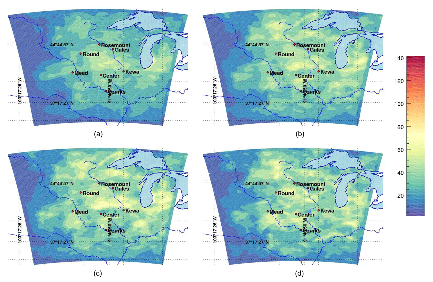
Figure 1Variances of CO2 in situ mole fractions (about 100 m a.g.l.) (in ppm2) using 25 members (a), 10 members (b), 8 members (c) and 5 members (d).
3.2 Filtering of sampling noise
We show here the values of the length scales in our filter resulting from the optimality criteria, applying both Gaussian (see Eq. 8) and non-Gaussian (see Eq. 10) filters to the raw variances. We implemented the dichotomy algorithm proposed in Ménétrier et al. (2015b) to obtain the optimal length scales of the filter, dividing (or multiplying) the length scale by a factor of 2 until convergence. The algorithm solves for the optimal length scale of the filter by scanning the space of solutions iteratively (applying a multiplicative factor at each time step to minimize the cost function). For all our cases, we defined the upper bound of the diagnosed length scale at 750 km, to represent about half the size of our simulation domain (square of 1600 km wide). This large value means that the extent of noisy structures would encompass the entire domain and therefore would not be recoverable. Here, the sampling noise is characterized by length scales of sizes ranging from a few kilometers to several hundred kilometers. In practice, the algorithm always converges but length scale might be larger than the domain size, meaning that all spatial structures in the variances are regarded as noise. This situation happens for two main reasons: spatial structures in the noise are similar to spatial gradients in the true variances, or the noise is larger than the true variances. Hence, the length scale falls beyond the limit of our simulation domain. In the method described by Ménétrier et al. (2015b), the ergodic assumption is necessary to diagnose robust estimators of the filter (see Sect. 2.2).
For CO2 mole fractions (see Fig. 2), the algorithm for the calibrated 25-member ensemble systematically converges to small length scales (<50 km), indicating that noise structures are very small in our optimal ensemble. When using the Gaussian filter, the algorithm systematically converges below our 750 km threshold for all cases except for 30 % of the days with the smallest ensemble (five members). In the non-Gaussian case, the filter converges to larger length scales beyond our threshold with the 5- and 10-member ensembles for less than 30 % of the days. Typically, length scales beyond our 750 km threshold are temporally coherent over periods of several days suggesting weather-related structures possibly inherited from synoptic-scale systems. These periods might be caused by high sampling noise compared to the true variances or by similar scales in spatial structures for both noise and true variances. Overall, the non-Gaussian filter shows a lower rate of convergence below 750 km compared to the Gaussian filter for CO2 mole fractions.
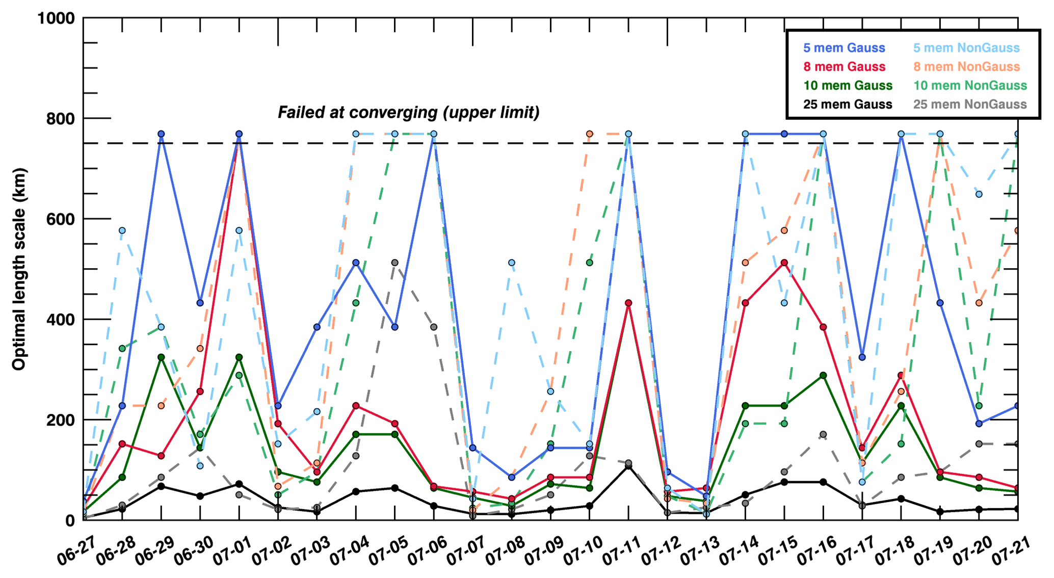
Figure 2Length scale (in km) of the variance filter for in situ CO2 mole fractions at about 100 m a.g.l. using Gaussian (solid lines) and non-Gaussian (dash lines) equations from 27 June to 21 July 2008.
For XCO2 column mole fractions (see Fig. 3), the optimal length scales are larger and the non-Gaussian filter converges beyond our threshold more frequently (about 50 % of the days for eight members or less). Even with the optimal 25-member ensembles, error structures of about 50 to 200 km are filtered out, significantly larger than for the CO2 mole fractions. We discuss in Sect. 4.2 the possible physical reasons behind these larger length scales, possibly due to large-scale structures in the free troposphere or to the complexity in noise structures as XCO2 data integrate noises from different altitudes. Figure 4 shows the results of the PBLH for which both filters converge beyond our threshold for half of the days in the Gaussian case. However, the filter converges more often below our threshold with the non-Gaussian filter applied to 10-member ensembles. Variance noise for PBLH present skewed distributions (not shown here) requiring the use of a non-Gaussian filter. We conclude here that 8- and 10-member ensembles are the minimum sizes with which sub-threshold convergence can be obtained on most days for most variables. Five-member ensembles will still be studied later on for covariances, as the localization of covariances does not depend on the filtered variances, but the low rate of convergence below 750 km might limit the use of the filtered variances.
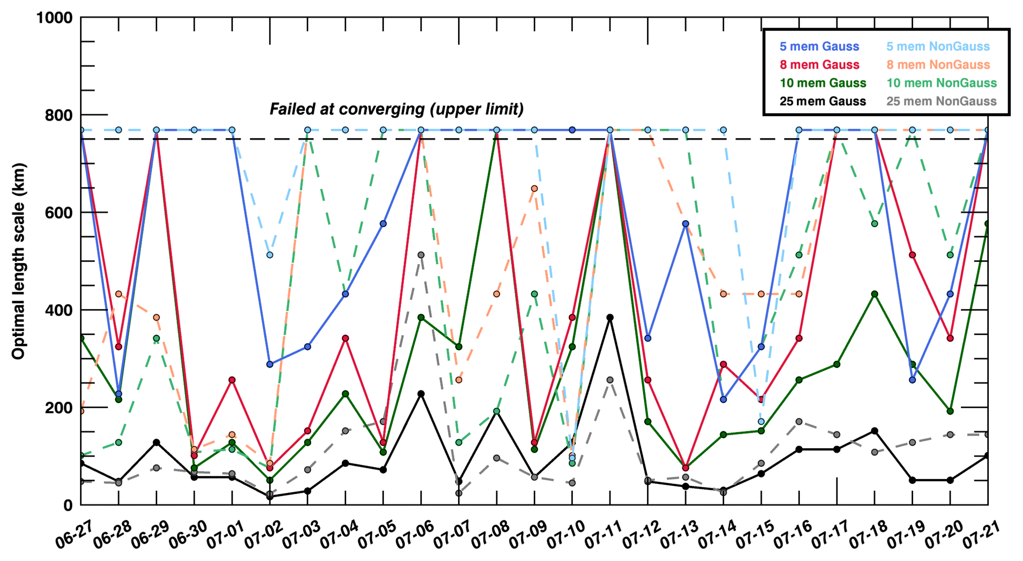
Figure 3Length scale (in km) of the variance filter for XCO2 total-column dry air mole fractions using Gaussian (solid lines) and non-Gaussian (dash lines) equations from 27 June to 21 July 2008.

Figure 4Length scale (in km) of the variance filter for planetary boundary layer heights using Gaussian (solid lines) and non-Gaussian (dash lines) equations from 27 June to 21 July 2008.
3.3 Variance filtering and ensemble sizes
The filtered variances shown in Fig. 5, here with the Gaussian filter, for the different ensemble sizes are in better agreement with the variances of the 25-member ensemble both in term of spatial patterns and magnitudes among the different ensembles. The filter successfully removed noisy structures, therefore decreasing the dependence on the number of members used in each case. Despite length scales beyond our threshold for 30 % of the days with the five-member ensemble, filtered variances at the monthly timescale show similar structures to 8- or 10-member ensembles, with nearly all of the noisy structures being removed by the filter. Compared to earlier results, the ensemble size does not seem to fundamentally limit the capacity of the filter to remove the noise, despite days with convergence beyond 750 km. The variance magnitude remains slightly larger for 10 members or less, with a relative overestimation of about 15 %. Our 5-member ensemble provided the best match with only 10 % higher than the 25-member filtered variances. The averaging over a whole month compensates for days with convergence beyond 750 km, producing reasonable estimates of the optimal variance even with five members. This result suggests that climatological error variances from small-size ensembles can be a good first approximation of the true variance when filtered correctly over most days.

Figure 5Monthly averages of the filtered variances of in situ CO2 mole fractions (about 100 m a.g.l.) (in ppm2) using 25 members (a), 10 members (b), 8 members (c) and 5 members (d).
3.4 Error variances in CO2, XCO2 and PBLH
We show in Fig. 6 the spatial distribution of error variances from the 25-member calibrated ensemble for in situ CO2 mole fractions in the planetary boundary layer (PBL; 100 m a.g.l.), in situ CO2 mole fractions in the free troposphere (about 5 km a.g.l.), total column of XCO2 dry air mole fractions and PBLH (in m a.g.l.). The four variables display very distinct spatial patterns. XCO2 variance spatial patterns (see Fig. 6c) exhibit distinct maximum values located in the eastern and southeastern part of the domain, whereas high CO2 variances are observed in the northeastern part of the domain for free-tropospheric CO2 (see Fig. 6b) or centrally located for CO2 variances in the PBL (see Fig. 6a). Finally, PBLH variances (see Fig. 6d) show no indication of direct relationship between large errors in the western part of the domain and the other three CO2 variables. We conclude here that no direct relationship can be utilized to construct CO2 variances based on PBLH. Similarly, maximum variances among the three CO2 variables are also significantly different in distribution and magnitudes.

Figure 6Filtered variances using the calibrated 25-member ensemble of in situ CO2 mole fractions at 100 m a.g.l. (in ppm2) (a), in situ CO2 mole fractions at 5 km a.g.l. (in ppm2) (b) XCO2 total dry air mole fractions (in ppm2) (c) and PBLH (in m2) (d).
3.5 Covariance localization: Schur and Wiener filters
Error covariances in CO2 mole fractions scale with the magnitude of the surface CO2 fluxes. They are therefore difficult to interpret. Instead, we present here the error correlations to highlight the spatial structures inherited from the transport models, independent of the magnitude of the underlying CO2 surface fluxes. We show in Fig. 7 the hourly correlation structures from the full 45-member ensemble (a–c) and our 25-member calibrated ensemble (d–f) at one of the instrumented towers in the US Midwest, i.e., Centerville, Iowa. We applied both Schur (see Fig. 7b, e) and Wiener (see Fig. 7c, f) filters to compare the impact of both filters on the raw correlations (see Fig. 7a, d). The Schur filter has less impact on the correlations compared to the Wiener filter which attenuates significantly the magnitude of the correlations for both ensembles. In Sect. 2.2, the local averaging of the optimal length scale assumes that the sampling noise is spatially homogeneous (third ingredient of the methods). This homogeneity assumption is required for the ergodicity assumption to apply, therefore yielding a domain-averaged filtering approach. The sub-domain used for the covariance filtering (here 400 km × 400 km) limits the spatial extent to 200 km around the observation location. The size of the domain was defined primarily for computational efficiency and based on the size of correlation structures, usually of about 100–200 km in length scale. To evaluate this assumption, we compared the size of the sub-domain to filter the covariances with a large area of 900 km × 900 km for the 45-member ensemble to a smaller area of 400 km × 400 km for the 25-member ensemble. Filtered correlations show similar results for Schur and slightly larger values for the smaller sub-domain when applying the Wiener filter. We conclude here that the spatial local averaging has a minor impact on the results and that our 25-member ensemble has similar spatial structures to the original 45-member ensemble, with larger correlations at short distances. We extend this analysis to the monthly timescale by showing monthly averaged error correlations, superimposed from different tower locations on the same map to aggregate the results at multiple locations (see Fig. 8). When averaged over longer timescales (see Fig. 8), the filtered correlations become isotropic, distributed around each location. The magnitudes remain larger with the Schur filter (see Fig. 8b) compared to the Wiener filter (see Fig. 8c) but the differences are noticeably smaller. The unfiltered correlations (see Fig. 8a) are noticeably larger due to noisy structures. After filtering, the spatial structures are distributed around the observation locations following a pseudo-Gaussian pattern. The magnitude of the error correlations, i.e., the length scale of the errors, is reduced in both cases compared to the raw correlations (see Fig. 8a). This result confirms that the sub-domain used here (400 km × 400 km) is sufficient to represent the error correlation structures around each measurement location and describes fully the error structures.
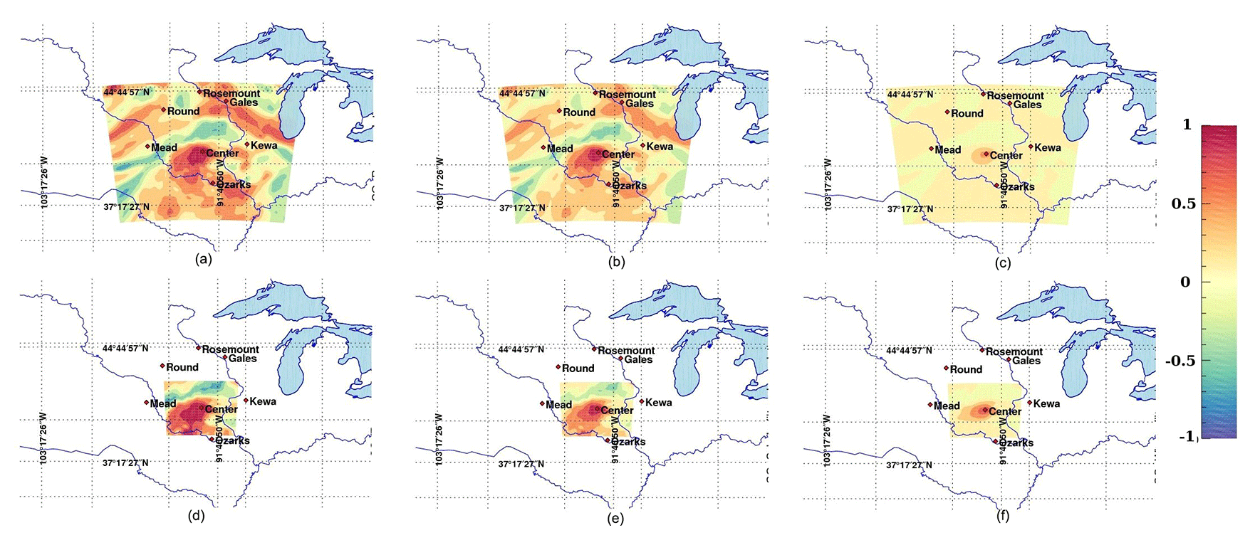
Figure 7Hourly raw (a, d) and filtered correlations using Schur (b, e) and Wiener (c, f) filtered correlations of in situ CO2 mole fractions at the Centerville tower (at about 100 m a.g.l.) on 26 June 2008. The correlations are based on the original 45-member ensemble (a, b, c) with a large subdomain (900 km × 900 km) and the 25-member ensemble (d, e, f) over the reference subdomain (400 km × 400 km). The highlighted domain also corresponds to the domain used for the spatial averaging of the correlations in the optimality conditions.
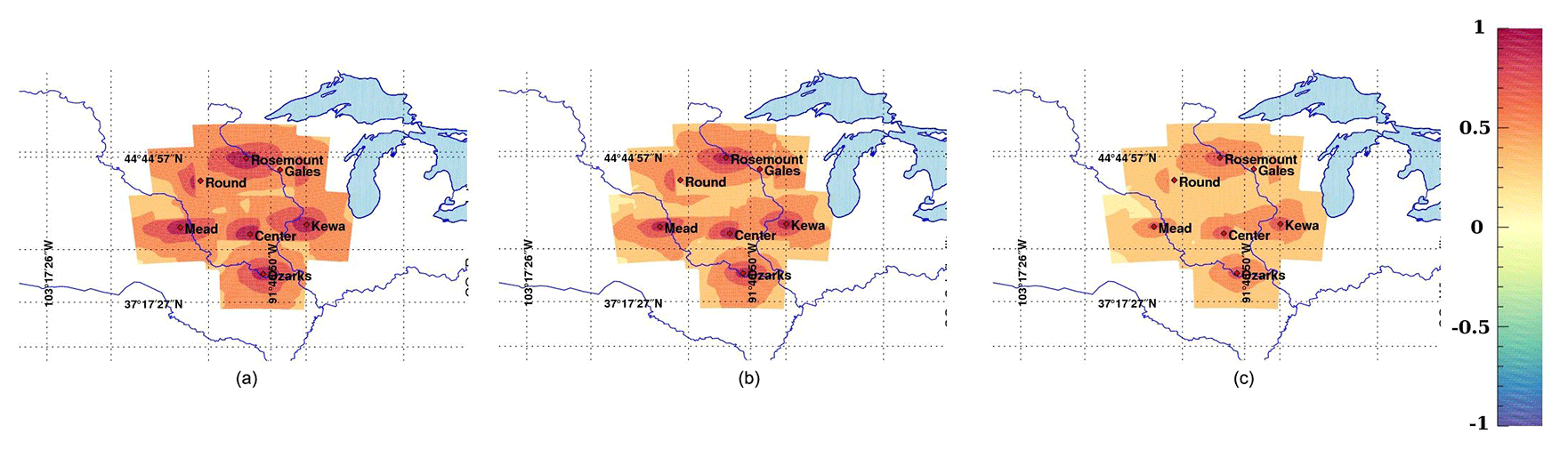
Figure 8Raw (a) and filtered correlations of CO2 in situ mole fractions at about 100 m a.g.l. based on 25 members using the Schur localization (b) and Wiener and Schur filter (c).
We show in Fig. 9 the results for the different ensemble sizes using the Schur filter. The 10- and 8-member ensembles show similar magnitude and patterns for the different sites, but the correlations are smaller than with the original ensemble. In comparison, the Wiener filter (see Fig. 10) generates consistent patterns with 25-, 10- and 8-member ensembles. In both cases, the filters decrease significantly the correlations in the five-member ensemble, revealing the inability of the filter to separate the noise from the actual error correlations. We present the localized correlation length scales for each tower and for each day in Fig. 12a. For both Center and Mead, length scales are noticeably larger than for the other towers and decrease rapidly until 2 July, before converging back to the same values diagnosed for other measurement sites. The differences across towers suggest local differences in error correlations, even across the same region for a single day (up to 70 km across our sites). These differences correspond to the beginning of summer, when both weather and ecosystem fluxes vary rapidly especially in agricultural areas. We discuss in Sect. 4.3 the relationship between meteorological and CO2 variables for both error variances and error correlations.
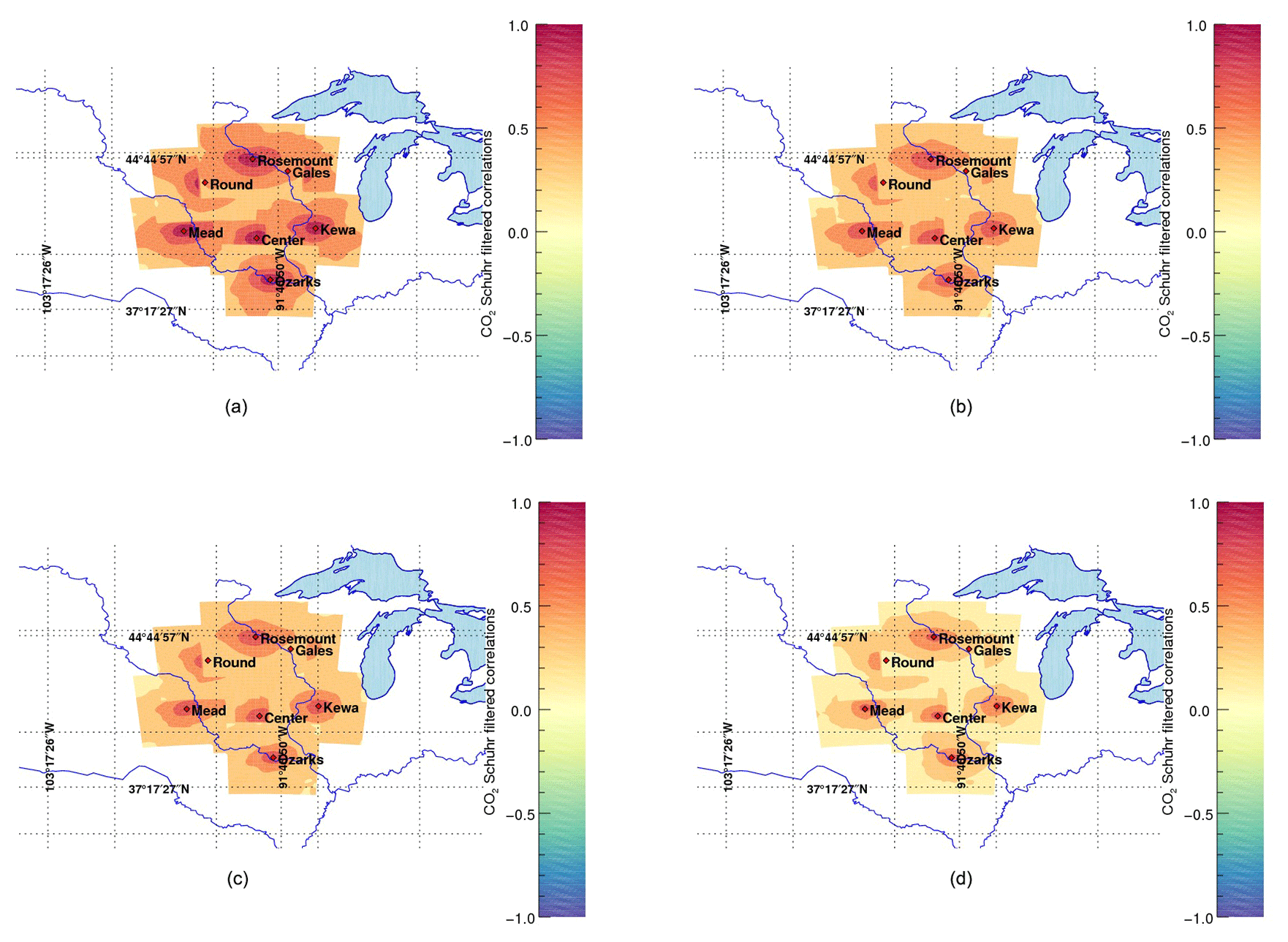
Figure 9Filtered correlations (using Schur product only) of CO2 in situ mole fractions (about 100 m a.g.l.) (in ppm2) (about 100 m a.g.l.) (in ppm2) using 25 members (a), 10 members (b), 8 members (c) and 5 members (d).

Figure 10Filtered correlations (using Wiener and Schur) of CO2 in situ mole fractions (about 100 m a.g.l.) (in ppm2) (about 100 m a.g.l.) (in ppm2) using 25 members (a), 10 members (b), 8 members (c) and 5 members (d).
4.1 Minimum size of calibrated ensembles
We discussed in Sect. 3.3 the dependence of the success of the variance filtering on the ensemble size. From these results, an ensemble of at least 8 to 10 members seems required to reach convergence below our 750 km convergence and hence filter the error variances. However, the spatial representation of the averaged filtered variances using a calibrated five-member ensemble (see Fig. 5) indicates a reasonable recovery of the error variances at the monthly timescale but not at the daily timescale. Theoretically, the minimum number of members for the covariance filtering is four, based on Eq. (11) with a factor (N−3) in the denominator, which shows that five-member ensembles are close to this limit and are not recommended in a more general context. The application here suggests 5-member ensembles are acceptable, but 8- to 10-member ensembles would be a minimum both in practice and in theory over different seasons and regions. Convergence beyond our threshold over single days has a limited impact on the monthly mean filtered variances. We conclude here that the filter produces satisfactory results to generate first-order estimates of the CO2 mole fraction errors. To achieve a systematic daily convergence below threshold, we recommend a larger number of members in the ensemble. One important point here is the calibration step performed before filtering, which optimizes the information content in each member relative to the other members. Therefore, a randomly generated ensemble may require additional members in order to represent the actual error variances. We tested the filtering technique on a random ensemble (i.e., uncalibrated) and found that beyond-threshold convergence is more frequent with 10 or less members (not shown here).
4.2 Impact of calibration on small-size ensembles
We have explored the impact of the calibration process on the error variances and covariances by filtering non-calibrated sub-ensembles of 8 and 10 members (see Fig. 11). These random ensembles have no member in common with their calibrated counterpart and are composed of simulations using various physics configuration randomly selected among the 45 original model configurations. The optimal length scale of the variance filter is systematically lower for non-calibrated ensembles (see Fig. 11, in gray and light blue) compared to calibrated ensembles (see Fig. 11, in black and royal blue), suggesting lower levels of noise with larger spatial structures, similar to larger ensemble sizes (25 members or more). Because members of the calibrated ensembles were selected to maximize the information content, calibrated-ensemble members differ more from each other than non-calibrated ensemble members. As shown in Díaz-Isaac et al. (2018a), one member with higher or lower PBLH statistics (usually the monthly mean model estimate) is systematically selected in order to generate calibrated ensembles with enough variance, and therefore capture the spatial and temporal variability in observed PBLH's from 14 radiosondes. Calibration might suggest different combinations of model physics for every single time period. In future studies, we recommend a combination of several preselected model physics with added perturbations to produce a sufficient ensemble spread but not perform the calibration for every time period. The calibration procedure might still be applied to existing ensembles but remain insufficient to sample the full spatial and temporal variability as discussed in Díaz-Isaac et al. (2018a). Some of these members introduce different spatial structures compared to the original ensemble, increasing the spread significantly. However, the small size of our ensembles with a larger variance may affect the sampling of these structures and hence our ability to differentiate noise from actual error structures. The approach proposed by Ménétrier et al. (2015a) was initially designed for ensembles with independently distributed members, which is not the case here. Some true correlation structures in the calibrated ensemble may be regarded as noise by the filter. Another approach would generate an ensemble based on the localized ensemble-based error covariance matrix. This approach will be developed further in future studies but is beyond the scope of this paper.
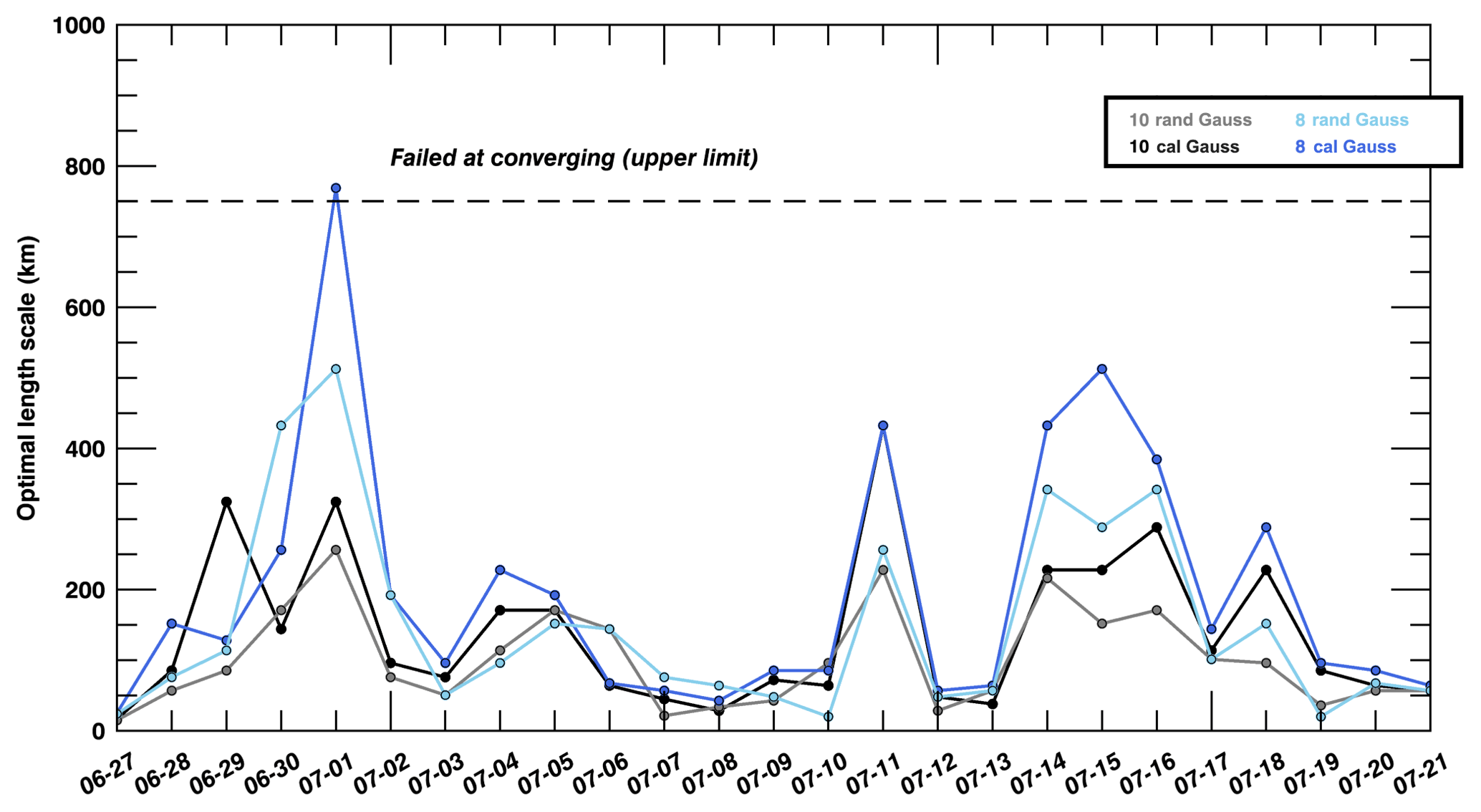
Figure 11Length scale (in km) of the Gaussian variance filter for 10-member random (in gray) and calibrated (in black) ensembles, and 8-member random (in light blue) and calibrated (royal blue) ensembles, for in situ CO2 mole fractions at about 100 m a.g.l. using Gaussian equations from 27 June to 21 July 2008.
4.3 Spatial structures in CO2 and meteorological errors
In Fig. 6, significant differences in filtered error variances were observed between in situ CO2 mole fractions (at different altitudes), XCO2 mole fractions and PBLH. Therefore, we conclude here that transport errors of meteorological variables are not transferable to CO2 and XCO2 error variances. This finding is in agreement with Miller et al. (2015), who found no direct relationship between errors in the meteorology and in situ CO2 mole fractions. However, considering the covariances, the spatial structures in CO2 mole fraction errors inherited from transport model errors exhibit well-defined patterns (e.g., Fig. 10). By fitting a simple Gaussian function in the form of to the filtered covariance fields, we diagnosed the characteristic length scale of the spatial error structures for the different variables, here CO2 100 m-high mole fractions, the mean horizontal zonal wind component and PBLH. Figure 12 shows the daily length scales at the seven measurement locations over the simulation period (i.e., 27 June to 21 July). The length scales L for the three variables increase rapidly between 27 June and 4 July from less than 100 to 150 km or higher. As there is no long-term spin-up (re-initialization of the perturbations every 5 d), the asymptotic behavior is most likely due to the seasonality of the errors from early to late summer. The seasonal changes in the atmospheric dynamics impact the spatial structures in the errors for the three variables. Across the seven sites, the characteristic length scale of spatial error structures also vary significantly, in particular for PBLH with large differences across sites. Both CO2 mole fractions and the mean zonal wind component reach a maximum value over July: respectively, 140 and 120 km. The comparison of the mean length scales (Fig. 12d) highlights the differences between the three variables. Both the CO2 100 m high mole fractions and the mean horizontal zonal wind component show similar variations and converge towards the same values but differ significantly from 29 June to 10 July. We conclude here that first-order estimates for CO2 spatial error correlations may be derived from meteorological error structures, in particular from the mean horizontal wind speed. But these approximations may be valid only for specific time periods. As presented in Sect. 3.4, error variances in CO2 and XCO2 mole fractions are decoupled from PBLH errors. Here, we suggest that error correlations may be derived from wind errors, but error variances should still be computed independently.
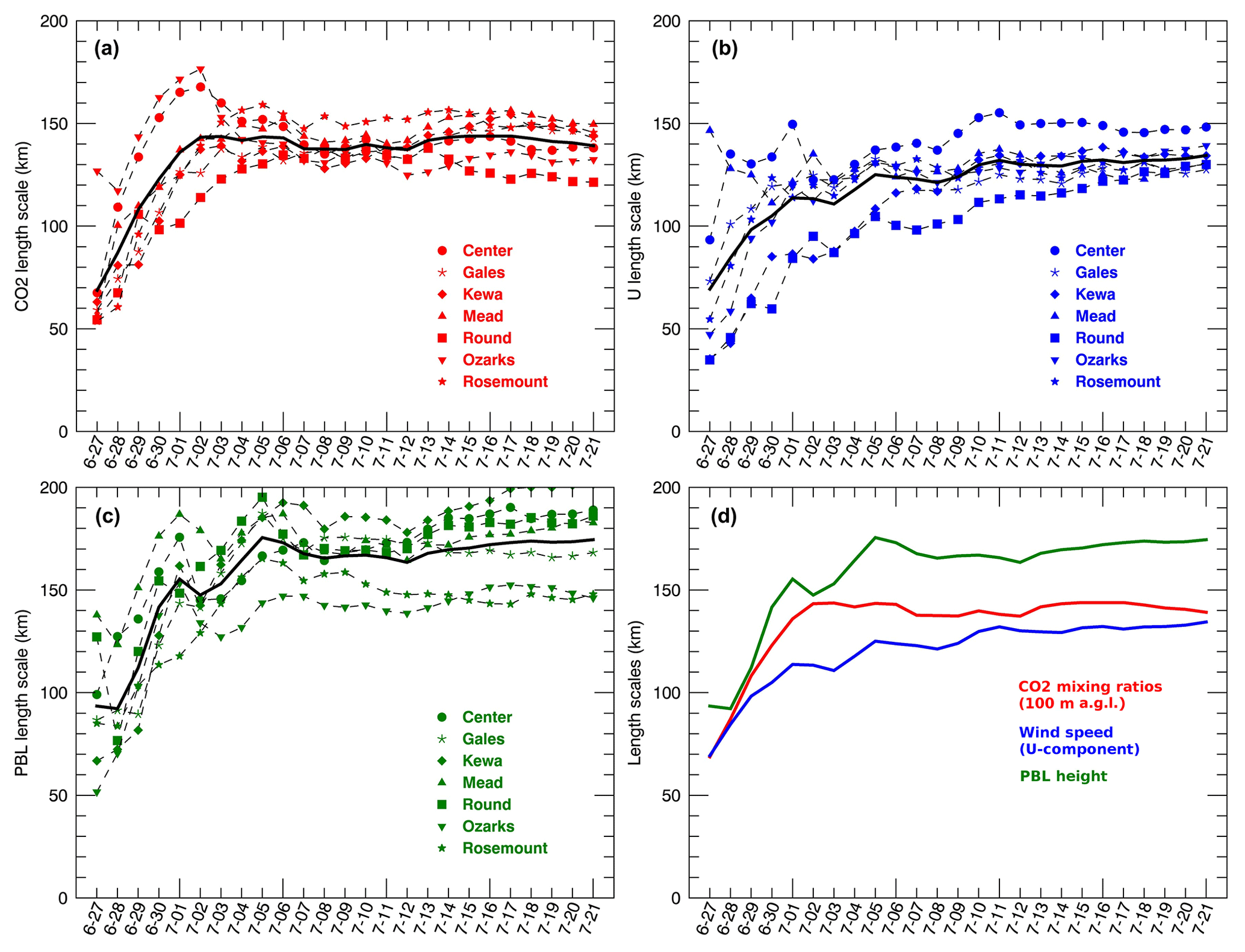
Figure 12Characteristic length scales L of filtered error correlations (from the 25-member ensemble) using an exponential function () for CO2 100 m high mole fractions (a), the mean horizontal zonal wind component (U; b), PBLH (c) and the mean values for the three variables (d) for every day of the simulation period (27 June to 21 July).
4.4 Evaluation and modeling of error correlations
This study presents a methodology to filter the noise in error structures from a small-size ensemble. The evaluation of the filtered structures would benefit from dense measurement campaigns sampling spatial structures across large domains, such as the Atmospheric Carbon and Transport (ACT)-America campaigns.2 Previous studies have shown the utility of aircraft measurements to diagnose error correlations (Gerbig et al., 2003), but the separation of spatial structures induced by surface flux errors and atmospheric transport errors remains challenging in order to construct observation error covariance matrices. The combination of ensemble systems such as ensemble Kalman filter (EnKF) systems and intensive aircraft campaigns will provide additional insights to evaluate filtering approaches (e.g., Chen et al., 2019). To introduce the findings of our study into an atmospheric inversion system, an additional step would be required in order to construct a regularized error covariance matrix. In this study, we acknowledge here that we have applied Schur and Wiener filters using the raw filtering matrices (Eqs. 9, 11 and 6), which may not produce semi-positive definite covariances. Future studies should include an additional step by adding a regularization of the covariances before filtering. For example, Lauvaux et al. (2009) proposed to model the error structures using a diffusion equation able to represent anisotropic structures, following the methodology described in Pannekoucke et al. (2008). Here, we presented a local filter able to remove the noise in the error structures. The diagnosed error structures can be approximated by different spatial functions of varying degrees of complexity, further regularized to generate positive–definite error covariance matrices. This next step is beyond the scope of this paper but will be conducted in the future to generate an efficient model of the corresponding error covariances based on our current results.
We have diagnosed the error variances and the spatial error structures from our mesoscale transport models at daily and monthly timescales. Applied to both CO2 mole fractions and meteorological variables, we implemented a cost-effective filtering technique currently used in meteorological data assimilation systems (Ménétrier et al., 2015b) to describe spatial error structures using a small-size ensemble. The approach remains affordable for multiyear inversions of sources and sinks at continental or regional scales. The removal of noisy structures in our small-size ensembles is evaluated by comparison with larger-size ensembles, both the original 45-member ensemble and our optimal calibrated sub-ensemble of 25 members. A second filtering approach for error covariances was successfully applied using the Wiener filter, producing similar results compared to the Schur filter over the 1-month simulation period. Differences were noticeable at shorter timescales (i.e., daily). The spatial distribution of error variances and spatial error structures are recoverable from small-size ensembles of 8 to 10 members, daily for in situ CO2 mole fractions and monthly for total-column XCO2, providing a more realistic representation of transport errors in future mesoscale inversions of CO2 fluxes. We noted that error variances of in situ CO2 mole fractions and total-column XCO2 differ significantly, even when varying the altitudes or considering PBLH error structures. We conclude that error variances for remote-sensing observations need to be quantified independently of PBL or free-tropospheric mole fractions.
We have discussed the potential use of meteorological error structures such as the mean horizontal wind to approximate spatial error correlations of in situ CO2 mole fractions. The seasonal variations in wind, PBLH and in situ CO2 mole fractions are highly correlated, while the typical length scales in error structures vary from 100 to 150 km in the middle of summer depending on the variable. We conclude here that meteorological error structures may provide a first-order estimation of correlation length scales in CO2 inversions when no ensemble of CO2 simulations is available.
The code is accessible under request by contacting the corresponding author (thomas.lauvaux@lsce.ipsl.fr).
The model simulation outputs are available under request by contacting the corresponding author (thomas.lauvaux@lsce.ipsl.fr).
In this study, we generate a reference ensemble to evaluate the sampling noise in the ensembles of smaller sizes. The original 45-member ensemble, uncalibrated, cannot be used as a reference as it underestimates model errors. Yet, the reference ensemble needs to include enough members to limit the sampling noise. Based on the same original ensemble of 45 members as in Díaz-Isaac et al. (2018a), we reduce it to a calibrated 25-member ensemble using the simulated annealing (SA) algorithm. The selection of the optimal calibrated ensemble is based on three meteorological variables (i.e., wind speed, wind direction and PBLH) and follows the same procedure described in Díaz-Isaac et al. (2018a). The SA for 25 members uses 40 000 iterations to reach convergence, significantly larger than the 20 000 iterations for 10-, 8- and 5-member ensembles. The same criterion used by Díaz-Isaac et al. (2018a) was applied to the selection process of the calibrated 25-member ensemble, improving the flatness of the rank histograms (Fig. A1). This selection is based on two criteria. First, we selected all the 25-member sub-ensembles with a rank histogram score smaller than six for each individual meteorological variable. In a second step, we filtered out the 25-member ensembles accepted by the SA algorithm but corresponding to a bias (i.e., mean model–data mismatch over 25 d) larger than the bias in the original 45-member ensemble. These criteria are applied to the three meteorological variables. This procedure is described in more detail in Díaz-Isaac et al. (2018a). The rank histograms in Fig. A1 show a limited under-dispersion of the 25-member ensemble, significantly reduced after calibration from 6.1, 6.2, 3.2 to 5.1, 4.9, and 2.5 for wind speed, wind direction and PBLH, respectively.
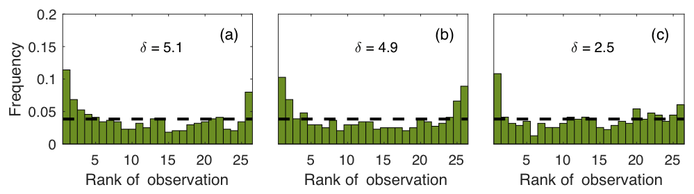
Figure A1Rank histograms of the 25-member ensemble after calibration for wind speed (a), wind direction (b) and planetary boundary layer height (c) over 35 d (18 June to 21 July 2008) using 14 rawinsonde sites available over the US Midwest. The horizontal dashed line corresponds to the ideal value for a flat rank histogram with respect to the number of members. The rank histogram score (δ) defines the flatness of the rank histogram, 1 being the ideal value.
The WRF-Chem simulations were performed by LIDI and TL; the filtering technique was coded by MB and TL based on the work of Benjamin Ménétrier; the concept and ideas were designed by MB, TL and NB; the paper was prepared by TL, LIDI, NB and MB.
The authors declare that they have no conflict of interest.
This research was supported by National Aeronautics and Space Administration (NASA) Terrestrial Ecosystem and Carbon Cycle Program (grant no. NNX11AE79G), by the NASA’s Earth Venture Program Atmospheric Carbon and Transport (ACT) – America (grant no. NNX15AG76G), by the Alfred P. Sloan Graduate Fellowship, by the NASA Carbon Monitoring System program (grant no. NNX13AP34G), and by the National Oceanic and Atmospheric Administration (grant no. NA14OAR4310136). CEREA is a member of Institut Pierre-Simon Laplace (IPSL).
This research has been supported by NASA (grant nos. NNX15AG76, NNX13AP34G, NNX15AI42G and NNX11AE79G) and NOAA (grant no. NA14OAR4310136).
This paper was edited by Christoph Gerbig and reviewed by Benjamin Ménétrier and one anonymous referee.
Anderson, J. L.: An ensemble adjustment Kalman filter for data assimilation, Mon. Weather Rev., 129, 2884–2903, 2001. a
Andrews, A. E., Kofler, J. D., Trudeau, M. E., Williams, J. C., Neff, D. H., Masarie, K. A., Chao, D. Y., Kitzis, D. R., Novelli, P. C., Zhao, C. L., Dlugokencky, E. J., Lang, P. M., Crotwell, M. J., Fischer, M. L., Parker, M. J., Lee, J. T., Baumann, D. D., Desai, A. R., Stanier, C. O., De Wekker, S. F. J., Wolfe, D. E., Munger, J. W., and Tans, P. P.: CO2, CO, and CH4 measurements from tall towers in the NOAA Earth System Research Laboratory's Global Greenhouse Gas Reference Network: instrumentation, uncertainty analysis, and recommendations for future high-accuracy greenhouse gas monitoring efforts, Atmos. Meas. Tech., 7, 647–687, https://doi.org/10.5194/amt-7-647-2014, 2014. a
Baker, D. F., Doney, S. C., and Schimel, D. S.: Variational data assimilation for atmospheric CO2, Tellus B, 58, 359–365, https://doi.org/10.1111/j.1600-0889.2006.00218.x, 2006. a
Baker, D. F., Law, R. M., Gurney, K. R., Rayner, P., Peylin, P., Denning, A. S., Bousquet, P., Bruhwiler, L., Chen, Y.-H., Ciais, P., Fung, I. Y., Heimann, M., John, J., Maki, T., Maksyutov, S., Masarie, K., Prather, M., Pak, B., Taguchi, S., and Zhu, Z.: TransCom 3 inversion intercomparison: Impact of transport model errors on the interannual variability of regional CO2 fluxes, 1988–2003, Global Biogeochem. Cy., 20, 439, https://doi.org/10.1029/2004GB002439, 2007. a
Brousseau, P., Berre, L., Bouttier, F., and Desroziers, G.: Flow-dependent background-error covariances for a convective-scale data assimilation system, Q. J. Roy. Meteor. Soc., 138, 310–322, https://doi.org/10.1002/qj.920, 2012. a
Bruhwiler, L. M. P., Michalak, A. M., Peters, W., Baker, D. F., and Tans, P.: An improved Kalman Smoother for atmospheric inversions, Atmos. Chem. Phys., 5, 2691–2702, https://doi.org/10.5194/acp-5-2691-2005, 2005. a
Chen, H. W., Zhang, F., Lauvaux, T., Davis, K. J., Feng, S., Butler, M. P., and Alley, R. B.: Characterization of Regional-Scale CO2 Transport Uncertainties in an Ensemble with Flow-Dependent Transport Errors, Geophys. Res. Lett., 46, 4049–4058, https://doi.org/10.1029/2018GL081341, 2019. a
Chevallier, F.: Impact of correlated observation errors on inverted CO2 surface fluxes from OCO measurements, Geophys. Res. Lett., 34, l24804, https://doi.org/10.1029/2007GL030463, 2007. a
Chevallier, F., Viovy, N., Reichstein, M., and Ciais, P.: On the assignment of prior errors in Bayesian inversions of CO2 surface fluxes, Geophys. Res. Lett., 33, l13802, https://doi.org/10.1029/2006GL026496, 2006. a
Chevallier, F., Ciais, P., Conway, T. J., Aalto, T., Anderson, B. E., Bousquet, P., Brunke, E. G., Ciattaglia, L., Esaki, Y., Fröhlich, M., Gomez, A., Gomez-Pelaez, A. J., Haszpra, L., Krummel, P. B., Langenfelds, R. L., Leuenberger, M., Machida, T., Maignan, F., Matsueda, H., Morguí, J. A., Mukai, H., Nakazawa, T., Peylin, P., Ramonet, M., Rivier, L., Sawa, Y., Schmidt, M., Steele, L. P., Vay, S. A., Vermeulen, A. T., Wofsy, S., and Worthy, D.: CO2 surface fluxes at grid point scale estimated from a global 21 year reanalysis of atmospheric measurements, J. Geophys. Res.-Atmos., 115, D21307, https://doi.org/10.1029/2010JD013887, 2010. a
Crisp, D., Atlas, R., Breon, F.-M., Brown, L., Burrows, J., Ciais, P., Connor, B., Doney, S., Fung, I., Jacob, D., Miller, C., O'Brien, D., Pawson, S., Randerson, J., Rayner, P., Salawitch, R., Sander, S., Sen, B., Stephens, G., Tans, P., Toon, G., Wennberg, P., Wofsy, S., Yung, Y., Kuang, Z., Chudasama, B., Sprague, G., Weiss, B., Pollock, R., Kenyon, D., and Schroll, S.: The Orbiting Carbon Observatory (OCO) mission, Adv. Space Res., 34, 700–709, https://doi.org/10.1016/j.asr.2003.08.062, 2004. a
De La Chevrotière, M. and Harlim, J.: A Data-Driven Method for Improving the Correlation Estimation in Serial Ensemble Kalman Filters, Mon. Weather Rev., 145, 985–1001, https://doi.org/10.1175/MWR-D-16-0109.1, 2017. a
Díaz-Isaac, L. I., Lauvaux, T., Davis, K. J., Miles, N. L., Richardson, S. J., Jacobson, A. R., and Andrews, A. E.: Model-data comparison of MCI field campaign atmospheric CO2 mole fractions, J. Geophys. Res.-Atmos., 119, 10536–10551, https://doi.org/10.1002/2014JD021593, 2014. a
Díaz-Isaac, L. I., Lauvaux, T., Bocquet, M., and Davis, K. J.: Calibration of a multi-physics ensemble for estimating the uncertainty of a greenhouse gas atmospheric transport model, Atmos. Chem. Phys., 19, 5695–5718, https://doi.org/10.5194/acp-19-5695-2019, 2019a. a, b, c, d, e, f, g, h, i, j, k, l, m, n
Díaz-Isaac, L. I., Lauvaux, T., and Davis, K. J.: Impact of physical parameterizations and initial conditions on simulated atmospheric transport and CO2 mole fractions in the US Midwest, Atmos. Chem. Phys., 18, 14813–14835, https://doi.org/10.5194/acp-18-14813-2018, 2018b. a
Engelen, R. J., Denning, A. S., and Gurney, K. R.: On error estimation in atmospheric CO2 inversions, J. Geophys. Res.-Atmos., 107, ACL10-1–ACL10-13, https://doi.org/10.1029/2002JD002195, 2002. a
Enting, I. G.: Inverse Problems in Atmospheric Constituent Transport, Cambridge University Press, Cambridge, 2002. a
Evensen, G.: Sequential data assimilation with a nonlinear quasi-geostrophic model using Monte Carlo methods to forecast error statistics, J. Geophys. Res.-Atmos., 99, 10143–10162, https://doi.org/10.1029/94JC00572, 1994. a
Evensen, G.: The Ensemble Kalman Filter: theoretical formulation and practical implementation, Ocean Dynam., 53, 343–367, https://doi.org/10.1007/s10236-003-0036-9, 2003. a
Feely, R. A., Wanninkhof, R., Takahashi, T., and Tans, P.: Influence of El Nino on the equatorial Pacific contribution to atmospheric CO2 accumulation, Nature, 398, 597–601, https://doi.org/10.1038/19273, 1999. a
Flowerdew, J.: Towards a theory of optimal localisation, Tellus A, 67, 25257, https://doi.org/10.3402/tellusa.v67.25257, 2015. a
Ganesan, A. L., Rigby, M., Zammit-Mangion, A., Manning, A. J., Prinn, R. G., Fraser, P. J., Harth, C. M., Kim, K.-R., Krummel, P. B., Li, S., Mühle, J., O'Doherty, S. J., Park, S., Salameh, P. K., Steele, L. P., and Weiss, R. F.: Characterization of uncertainties in atmospheric trace gas inversions using hierarchical Bayesian methods, Atmos. Chem. Phys., 14, 3855–3864, https://doi.org/10.5194/acp-14-3855-2014, 2014. a
Garaud, D. and Mallet, V.: Automatic calibration of an ensemble for uncertainty estimation and probabilistic forecast: Application to air quality, J. Geophys. Res.-Atmos., 116, d19304, https://doi.org/10.1029/2011JD015780, 2011. a
Gerbig, C., Lin, J. C., Wofsy, S. C., Daube, B. C., Andrews, A. E., Stephens, B. B., Bakwin, P. S., and Grainger, C. A.: Toward constraining regional-scale fluxes of CO2 with atmospheric observations over a continent: 1. Observed spatial variability from airborne platforms, J. Geophys. Res.-Atmos., 108, 4756, https://doi.org/10.1029/2002JD003018, 2003. a
Gurney, K. R., Law, R. M., Denning, A. S., Rayner, P. J., Baker, D., Bousquet, P., Bruhwiler, L., Chen, Y.-H., Ciais, P., Fan, S., Fung, I. Y., Gloor, M., Heimann, M., Higuchi, K., John, J., Maki, T., Maksyutov, S., Masarie, K., Peylin, P., Prather, M., Pak, B. C., Randerson, J., Sarmiento, J., Taguchi, S., Takahashi, T., and Yuen, C.-W.: Towards robust regional estimates of CO2 sources and sinks using atmospheric transport models, Nature, 415, 626–630, 2002. a
Hamill, T. M., Whitaker, J. S., and Snyder, C.: Distance-Dependent Filtering of Background Error Covariance Estimates in an Ensemble Kalman Filter, Mon. Weather Rev., 129, 2776–2790, https://doi.org/10.1175/1520-0493(2001)129<2776:DDFOBE>2.0.CO;2, 2001. a
Hilton, T. W., Davis, K. J., Keller, K., and Urban, N. M.: Improving North American terrestrial CO2 flux diagnosis using spatial structure in land surface model residuals, Biogeosciences, 10, 4607–4625, https://doi.org/10.5194/bg-10-4607-2013, 2013. a
Houtekamer, P. L. and Mitchell, H. L.: Data Assimilation Using an Ensemble Kalman Filter Technique, Mon. Weather Rev., 126, 796–811, https://doi.org/10.1175/1520-0493(1998)126<0796:DAUAEK>2.0.CO;2, 1998. a
Houtekamer, P. L. and Mitchell, H. L.: A Sequential Ensemble Kalman Filter for Atmospheric Data Assimilation, Mon. Weather Rev., 129, 123–137, https://doi.org/10.1175/1520-0493(2001)129<0123:ASEKFF>2.0.CO;2, 2001. a, b
Houweling, S., Baker, D., Basu, S., Boesch, H., Butz, A., Chevallier, F., Deng, F., Dlugokencky, E. J., Feng, L., Ganshin, A., Hasekamp, O., Jones, D., Maksyutov, S., Marshall, J., Oda, T., O'Dell, C. W., Oshchepkov, S., Palmer, P. I., Peylin, P., Poussi, Z., Reum, F., Takagi, H., Yoshida, Y., and Zhuravlev, R.: An intercomparison of inverse models for estimating sources and sinks of CO2 using GOSAT measurements, J. Geophys. Res.-Atmos., 120, 5253–5266, https://doi.org/10.1002/2014JD022962, 2015. a
IPCC: Carbon and Other Biogeochemical Cycles, in: Climate Change 2013: The Physical Science Basis. Contribution of Working Group I to the Fifth Assessment Report of the Intergovernmental Panel on Climate Change, edited by: Stocker, T. F., Qin, D., Plattner, G.-K., Tignor, M., Allen, S. K., Boschung, J., Nauels, A., Xia, Y., Bex, V., and Midgley, P. M., Cambridge University Press, Cambridge, UK and New York, NY, USA, 2015. a
Jankov, I., Berner, J., Beck, J., Jiang, H., Olson, J. B., Grell, G., Smirnova, T. G., Benjamin, S. G., and Brown, J. M.: A Performance Comparison between Multiphysics and Stochastic Approaches within a North American RAP Ensemble, Mon. Weather Rev., 145, 1161–1179, https://doi.org/10.1175/MWR-D-16-0160.1, 2017. a
Keenan, T. F., Prentice, I. C., Canadell, J. G., Williams, C. A., Wang, H., Raupach, M., and Collatz, G. J.: Recent pause in the growth rate of atmospheric CO2 due to enhanced terrestrial carbon uptake, Nat. Commun., 7, 13428, https://doi.org/10.1038/ncomms13428, 2016. a
Kim, J.-S., Kug, J.-S., Yoon, J.-H., and Jeong, S.-J.: Increased Atmospheric CO2 Growth Rate during El Niño Driven by Reduced Terrestrial Productivity in the CMIP5 ESMs, J. Climate, 29, 8783–8805, https://doi.org/10.1175/JCLI-D-14-00672.1, 2016. a
Lauvaux, T., Pannekoucke, O., Sarrat, C., Chevallier, F., Ciais, P., Noilhan, J., and Rayner, P. J.: Structure of the transport uncertainty in mesoscale inversions of CO2 sources and sinks using ensemble model simulations, Biogeosciences, 6, 1089–1102, https://doi.org/10.5194/bg-6-1089-2009, 2009. a, b, c
Lauvaux, T., Schuh, A. E., Uliasz, M., Richardson, S., Miles, N., Andrews, A. E., Sweeney, C., Diaz, L. I., Martins, D., Shepson, P. B., and Davis, K. J.: Constraining the CO2 budget of the corn belt: exploring uncertainties from the assumptions in a mesoscale inverse system, Atmos. Chem. Phys., 12, 337–354, https://doi.org/10.5194/acp-12-337-2012, 2012. a, b
Lauvaux, T., Miles, N. L., Deng, A., Richardson, S. J., Cambaliza, M. O., Davis, K. J., Gaudet, B., Gurney, K. R., Huang, J., O'Keefe, D., Song, Y., Karion, A., Oda, T., Patarasuk, R., Razlivanov, I., Sarmiento, D., Shepson, P., Sweeney, C., Turnbull, J., and Wu, K.: High-resolution atmospheric inversion of urban CO2 emissions during the dormant season of the Indianapolis Flux Experiment (INFLUX), J. Geophys. Res.-Atmos., 121, 5213–5236, https://doi.org/10.1002/2015JD024473, 2016. a, b
Le Quéré, C., Andrew, R. M., Canadell, J. G., Sitch, S., Korsbakken, J. I., Peters, G. P., Manning, A. C., Boden, T. A., Tans, P. P., Houghton, R. A., Keeling, R. F., Alin, S., Andrews, O. D., Anthoni, P., Barbero, L., Bopp, L., Chevallier, F., Chini, L. P., Ciais, P., Currie, K., Delire, C., Doney, S. C., Friedlingstein, P., Gkritzalis, T., Harris, I., Hauck, J., Haverd, V., Hoppema, M., Klein Goldewijk, K., Jain, A. K., Kato, E., Körtzinger, A., Landschützer, P., Lefèvre, N., Lenton, A., Lienert, S., Lombardozzi, D., Melton, J. R., Metzl, N., Millero, F., Monteiro, P. M. S., Munro, D. R., Nabel, J. E. M. S., Nakaoka, S., O'Brien, K., Olsen, A., Omar, A. M., Ono, T., Pierrot, D., Poulter, B., Rödenbeck, C., Salisbury, J., Schuster, U., Schwinger, J., Séférian, R., Skjelvan, I., Stocker, B. D., Sutton, A. J., Takahashi, T., Tian, H., Tilbrook, B., van der Laan-Luijkx, I. T., van der Werf, G. R., Viovy, N., Walker, A. P., Wiltshire, A. J., and Zaehle, S.: Global Carbon Budget 2016, Earth Syst. Sci. Data, 8, 605–649, https://doi.org/10.5194/essd-8-605-2016, 2016. a
Lei, L. and Anderson, J. L.: Comparisons of Empirical Localization Techniques for Serial Ensemble Kalman Filters in a Simple Atmospheric General Circulation Model, Mon. Weather Rev., 142, 739–754, https://doi.org/10.1175/MWR-D-13-00152.1, 2014. a
McKain, K., Down, A., Raciti, S. M., Budney, J., Hutyra, L. R., Floerchinger, C., Herndon, S. C., Nehrkorn, T., Zahniser, M. S., Jackson, R. B., Phillips, N., and Wofsy, S. C.: Methane emissions from natural gas infrastructure and use in the urban region of Boston, Massachusetts, P. Natl. Acad. Sci. USA, 112, 1941–1946, https://doi.org/10.1073/pnas.1416261112, 2015. a
Ménétrier, B., Montmerle, T., Michel, Y., and Berre, L.: Linear Filtering of Sample Covariances for Ensemble-Based Data Assimilation. Part I: Optimality Criteria and Application to Variance Filtering and Covariance Localization, Mon. Weather Rev., 143, 1622–1643, https://doi.org/10.1175/MWR-D-14-00157.1, 2015a. a, b, c, d, e, f, g, h, i, j
Ménétrier, B., Montmerle, T., Michel, Y., and Berre, L.: Linear Filtering of Sample Covariances for Ensemble-Based Data Assimilation. Part II: Application to a Convective-Scale NWP Model, Mon. Weather Rev., 143, 1644–1664, 2015b. a, b, c, d, e
Miles, N. L., Richardson, S. J., Davis, K. J., Lauvaux, T., Andrews, A. E., West, T. O., Bandaru, V., and Crosson, E. R.: Large amplitude spatial and temporal gradients in atmospheric boundary layer CO2 mole fractions detected with a tower-based network in the U.S. upper Midwest, J. Geophys. Res.-Biogeo., 117, G01019, https://doi.org/10.1029/2011JG001781, 2012. a
Miller, S. M., Hayek, M. N., Andrews, A. E., Fung, I., and Liu, J.: Biases in atmospheric CO2 estimates from correlated meteorology modeling errors, Atmos. Chem. Phys., 15, 2903–2914, https://doi.org/10.5194/acp-15-2903-2015, 2015. a, b
Pannekoucke, O., Berre, L., and Desroziers, L.: Background error correlation length-scale estimates and their sampling statistics, Q. J. Roy. Meteor. Soc., 134, 497–508, 2008. a, b
Peters, W., Jacobson, A. R., Sweeney, C., Andrews, A. E., Conway, T. J., Masarie, K., Miller, J. B., Bruhwiler, L. M. P., Pétron, G., Hirsch, A. I., Worthy, D. E. J., van der Werf, G. R., Randerson, J. T., Wennberg, P. O., Krol, M. C., and Tans, P. P.: An atmospheric perspective on North American carbon dioxide exchange: CarbonTracker, P. Natl. Acad. Sci. USA, 104, 18925–18930, https://doi.org/10.1073/pnas.0708986104, 2007. a
Peylin, P., Law, R. M., Gurney, K. R., Chevallier, F., Jacobson, A. R., Maki, T., Niwa, Y., Patra, P. K., Peters, W., Rayner, P. J., Rödenbeck, C., van der Laan-Luijkx, I. T., and Zhang, X.: Global atmospheric carbon budget: results from an ensemble of atmospheric CO2 inversions, Biogeosciences, 10, 6699–6720, https://doi.org/10.5194/bg-10-6699-2013, 2013. a, b
Raynaud, L. and Pannekoucke, O.: Sampling properties and spatial filtering of ensemble background-error length-scales, Q. J. Roy. Meteor. Soc., 139, 784–794, https://doi.org/10.1002/qj.1999, 2013. a
Rayner, P. J. and O'Brien, D. M.: The utility of remotely sensed CO2 concentration data in surface source inversions, Geophys. Res. Lett., 28, 175–178, 2001. a
Schimel, D., Stephens, B. B., and Fisher, J. B.: Effect of increasing CO2 on the terrestrial carbon cycle, P. Natl. Acad. Sci. USA, 112, 436–441, https://doi.org/10.1073/pnas.1407302112, 2015. a
Skamarock, W. C., Klemp, J. B., Dudhia, J., Gill, D. O., Barker, D. M., Duda, M. G., Huang, X.-Y., Wang, W., and Powers, J. G.: A Description of the Advanced Research WRF Version 3, National Center of Atmospheric Research, Tech. Note, NCAR/TN-475+STR, 113 pp., 2008. a
Stephens, B. B., Gurney, K. R., Tans, P. P., Sweeney, C., Peters, W., Bruhwiler, L., Ciais, P., Ramonet, M., Bousquet, P., Nakazawa, T., Aoki, S., Machida, T., Inoue, G., Vinnichenko, N., Lloyd, J., Jordan, A., Heimann, M., Shibistova, O., Langenfelds, R. L., Steele, L. P., Francey, R. J., and Denning, A. S.: Weak Northern and Strong Tropical Land Carbon Uptake from Vertical Profiles of Atmospheric CO2, Science, 316, 1732–1735, https://doi.org/10.1126/science.1137004, 2007. a
Viatte, C., Lauvaux, T., Hedelius, J. K., Parker, H., Chen, J., Jones, T., Franklin, J. E., Deng, A. J., Gaudet, B., Verhulst, K., Duren, R., Wunch, D., Roehl, C., Dubey, M. K., Wofsy, S., and Wennberg, P. O.: Methane emissions from dairies in the Los Angeles Basin, Atmos. Chem. Phys., 17, 7509–7528, https://doi.org/10.5194/acp-17-7509-2017, 2017. a
Wu, L., Bocquet, M., Chevallier, F., Lauvaux, T., and Davis, K.: Hyperparameter estimation for uncertainty quantification in mesoscale carbon dioxide inversions, Tellus B, 65, 20894, https://doi.org/10.3402/tellusb.v65i0.20894, 2013. a
Yokota, T., Yoshida, Y., Eguchi, N., Ota, Y., Tanaka, T., Watanabe, H., and Maksyutov, S.: Global Concentrations of CO2 and CH4 Retrieved from GOSAT: First Preliminary Results, SOLA, 5, 160–163, https://doi.org/10.2151/sola.2009-041, 2009. a
http://www.esrl.noaa.gov/gmd/ccgg/trends/, last access: 29 August 2019.
https://www-air.larc.nasa.gov/missions/ACT-America/, last access: 4 July 2018.