the Creative Commons Attribution 4.0 License.
the Creative Commons Attribution 4.0 License.
 | 10 Sep 2019
A double ITCZ phenomenology of wind errors in the equatorial Atlantic in seasonal forecasts with ECMWF models
Jonathan K. P. Shonk
Teferi D. Demissie
Thomas Toniazzo
Modern coupled general circulation models produce systematic biases in the tropical Atlantic that hamper the reliability of long-range predictions. This study focuses on a common springtime westerly wind bias in the equatorial Atlantic in seasonal hindcasts from two coupled models – ECMWF System 4 and EC-Earth v2.3 – and in hindcasts also based on System 4, but with prescribed sea-surface temperatures.
The development of the equatorial westerly bias in early April is marked by a rapid transition from a wintertime easterly, cold tongue bias to a springtime westerly bias regime that displays a marked double intertropical convergence zone (ITCZ). The transition is a seasonal feature of the model climatology (independent of initialisation date) and is associated with a seasonal increase in rainfall where a second branch of the ITCZ is produced south of the Equator. Excess off-equatorial convergence redirects the trade winds away from the Equator. Based on arguments of temporal coincidence, the results of our analysis contrast with those from previous work, and alleged causes hereto identified as the likely cause of the equatorial westerly bias in other models must be discarded. Quite in general, we find no evidence of remote influences on the development of the springtime equatorial bias in the Atlantic in the IFS-based models. Limited evidence however is presented that supports the hypothesis of an incorrect representation of the meridional equatorward flow in the marine boundary layer of the southern Atlantic as a contributing factor. Erroneous dynamical constraints on the flow upstream of the Equator may generate convergence and associated rainfall south of the Equator. This directs attention to the representation of the properties of the subtropical boundary layer as a potential source for the double ITCZ bias.
- Article
(12395 KB) - Full-text XML
- BibTeX
- EndNote


The identification and reduction of systematic biases in coupled general circulation models (CGCMs) have been ongoing challenges in model development in recent times. Despite significant development of CGCMs in the last two decades, large systematic biases remain in the simulated tropical climate – including the tropical Atlantic (Solomon et al., 2007; Davey et al., 2002; Richter and Xie, 2008; Toniazzo and Woolnough, 2014). These biases can have significant impacts on seasonal forecasts and future climate predictions. A common problem is the misrepresentation of the annual mean zonal gradient of sea-surface temperature (SST) over the equatorial Atlantic, with a tendency for models to simulate colder SSTs in the west and warmer SSTs in the east (Davey et al., 2002; Klein et al., 2013; Richter et al., 2014). This reversed gradient is at least partly due to the failure of CGCMs to reproduce the observed cold tongue (a region of colder water extending along the equatorial Atlantic from the east) and the associated shallow mixed layer in the eastern equatorial Atlantic during boreal summer (Davey et al., 2002; Richter and Xie, 2008). In turn, this has been shown to be associated with, and in some cases the result of, a westerly equatorial surface wind bias that develops during boreal spring (Chang et al., 2007; Richter et al., 2012, 2014). The erroneous seasonal slackening of the equatorial easterlies also has significant implications for the coastal climate of south-west Africa, where a systematic warm bias develops in CGCMs partly in response to wind-forced equatorial thermocline anomalies that propagate poleward along the coast (Toniazzo and Woolnough, 2014; Voldoire et al., 2014, 2019).
A number of hypotheses have been proposed for the possible root causes of the springtime surface westerly wind bias over the equatorial Atlantic. Several studies have suggested root causes in the ocean models, such as erroneous stratification and insufficient upwelling in the cold tongue (Breugem et al., 2008; Exarchou et al., 2018) and poorly resolved dynamical features associated with a model grid that is too coarse (Seo et al., 2006). However, an equatorial westerly bias is a common feature of atmospheric GCM (AGCM) simulations with prescribed SSTs (Richter and Xie, 2008), suggesting the coupled intensification of an atmospheric bias. Chang et al. (2008), Wahl et al. (2011) and Richter et al. (2012) showed that the westerly bias is associated with biases in sea-level pressure gradient in the atmosphere component and rainfall biases in the Amazon and West Africa. However, a direct causal link between these concomitant model biases was not clearly established.
It is important to identify the most prevalent causes of the development of the westerly bias, since it is linked with a failure to correctly simulate the mean seasonal cycle of equatorial winds and SST, which affects the ability of CGCMs to predict tropical Atlantic variability such as the Atlantic Niño (Dippe et al., 2018). Also, as a result of the warm SST biases on the Equator and along the coast, the simulation of the present and future climate may be regarded as unreliable, especially if employed to forecast rainfall over decadal and seasonal timescales in the tropical Atlantic and the adjoining continental monsoon areas (Hulme et al., 2001). Linking systematic biases with process errors in the models can help to improve not only their performance but also the initialisation procedures for seasonal-to-decadal forecast applications, which would ultimately lead to a more skilful forecast over the tropical Atlantic.
In this study, we analyse systematic biases in the tropical Atlantic in seasonal hindcasts (also sometimes referred to as reforecasts) obtained with the System 4 coupled seasonal prediction system of the European Centre for Medium-Range Weather Forecasts (ECMWF). These are compared with hindcasts obtained by prescribing the time-dependent SST fields from observations in order to isolate biases originating from the atmosphere component of the model and those originating from air–sea coupling. We also compare the results with hindcasts based on the coupled EC-Earth v2.3 model in order to assess the dependence of biases over the equatorial Atlantic on model physics and on biases occurring elsewhere. The analysis methodology is similar to that adopted by Shonk et al. (2018) and Toniazzo and Woolnough (2014), in that clues on the causal links between different biases are derived from the temporal sequence with which they appear in the course of the hindcasts, as well as on the relationship, or lack thereof, with more or less evolved SST biases. Using this methodology, we probe the origins of the springtime westerly zonal wind bias in an attempt to build an understanding of the processes that lead to its development and ultimately hypothesise where its root cause may lie. In the next section of this paper we introduce the models in more detail and describe the datasets. In Sect. 3, we describe the evolution of systematic hindcast biases in the Atlantic basin. In Sect. 4, we investigate the relationship of such biases with biases that develop outside the tropical Atlantic. In Sect. 5, we discuss some hypotheses of bias origins based on the results from the previous two sections. We conclude the paper in Sect. 6.
We use hindcast data from two models in this study. The first is ECMWF System 4 (referred to as “S4” in this paper), a model designed for operational seasonal forecasting; the second is EC-Earth version 2.3 (“EC”), a model designed as a tool for climate research. S4 combines cycle 36R4 of the Integrated Forecast System (IFS; Molteni et al., 2011) with version 3.0 of the Nucleus for European Modelling of the Ocean (NEMO; Madec, 2008), coupled using a version of the Ocean Atmosphere Sea Ice Soil 3 coupler (OASIS3; Valcke, 2013). The IFS's dynamical core uses a spectral horizontal discretisation and hybrid sigma-p levels in the vertical. Cycle 36R4 has a quadratic truncation at wavenumber 255 on 91 vertical levels that extend from the surface to 0.01 hPa. The physics calculations are made on a Gaussian N128 grid, giving a horizontal resolution of about 0.7∘. The NEMO ocean component uses a finite-difference discretisation on the curvilinear ORCA1 grid, which has a horizontal resolution of about 1∘ (with increased meridional resolution at the Equator) and 42 levels in the vertical.
The EC model also uses the IFS atmosphere model but cycle 31R1. It is truncated at wavenumber 159 and has 62 levels up to 5 hPa; the physical parameterisations are computed on a reduced Gaussian N80 grid, corresponding to a horizontal resolution of 1.125∘. EC uses version 2.0 of NEMO as its ocean component, which runs on the same ORCA1 grid as the version of NEMO in S4, and OASIS3 for coupling. Table 1 presents a summary of the differences between the two models. Full details on S4 and EC are presented by Molteni et al. (2011) and Hazeleger et al. (2010, 2012) respectively.
Table 1Summary of the main features of the two coupled models used in this study. The features of the uncoupled model S4A are the same as S4, but with the SST prescribed and hence no ocean component.
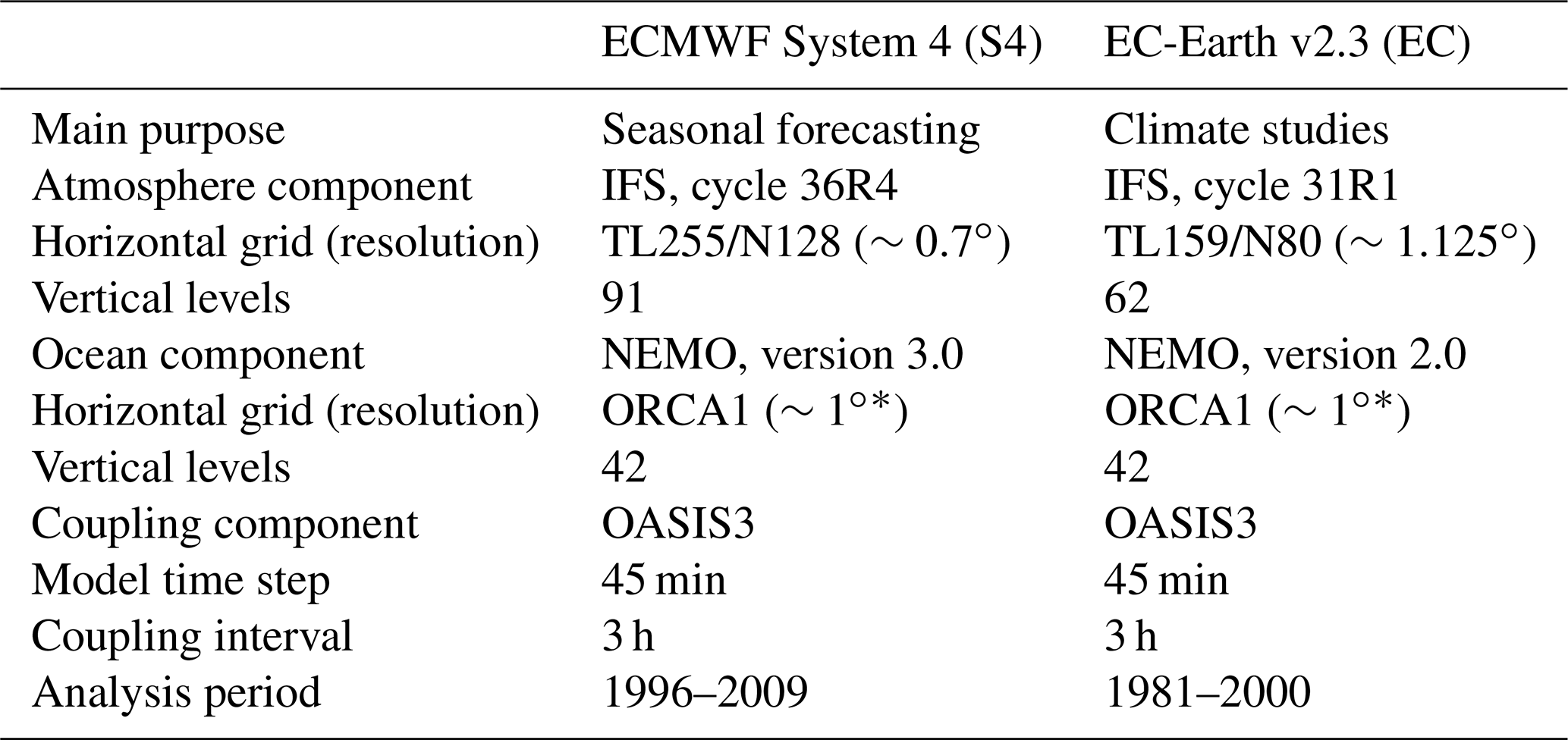
* Increased meridional resolution at the Equator – up to about 1∕3∘.
Operational hindcasts are available from S4 starting on the first of every month and run for at least 7 months; hindcasts are available from EC starting on 1 February, 1 May, 1 August and 1 November and run for 4 months. A further set of hindcasts is available from an atmosphere-only version of S4, which we refer to as “S4A”. This uses the same version of the IFS as S4, but with SST prescribed from the OISST dataset (Reynolds et al., 2002). The S4A hindcasts are initialised on the same four dates in the year as the EC hindcasts and are also run for 4 months.
For the hindcast climatologies of S4 and S4A, we select a subset of 14 years, spanning 1996 to 2009; for EC, we select a 20-year period spanning 1981 to 2000. During these periods, both S4 and EC are initialised with atmosphere data from ERA-Interim (Dee et al., 2011) and ocean data from ORA-S4 (Balmaseda et al., 2013). We preclude years more recent than 2009 in S4 and S4A as, from 2010 onwards, initial conditions are obtained from operational analyses instead of ERA-Interim. For EC, we preclude years after 2000 as, from 2001 onwards, there was a change in the initialisation method. Hence, for all models, these ranges represent the most up-to-date range of years available with a consistent initialisation data source and method. For S4 and S4A, we extract eight ensemble members for each start date, as this was found to be sufficient to represent model uncertainty. For EC, we use all 10 ensemble members that are available. Ensemble means are used throughout to represent the models' best estimates of the conditions.
Our observation datasets have been selected to match the initialisation datasets where possible. We take SST observations from OISST and wind observations from ERA-Interim. Observed rainfall is taken from the Tropical Rainfall Measuring Mission (TRMM; Kummerow et al., 2000). As in Toniazzo and Woolnough (2014) and Shonk et al. (2018), we base the analysis of systematic biases and their evolution on the comparison between climatologies from the hindcasts (one daily or monthly mean climatology for each lead time in the hindcast) with a corresponding daily or monthly mean climatology from the observations. Where possible, these climatologies have been constructed from matching subsets of years (validity time in the hindcasts) in order to minimise bias contributions originating from observed and simulated interannual variability. However, when the overlap between years in different datasets is limited, we deviate from this rule. In any case, in this analysis we focus on systematic biases only, and we have ensured that none of the results presented here is sensitive to details of the time period chosen to define the climatologies. Where statistical significance is calculated for a certain mean bias, this is obtained by considering the statistical distribution of that bias in the available ensemble of hindcasts.
3.1 Annual cycle of climatological biases
The biases in the seasonal climatology of S4 hindcasts, defined as the average bias in the seventh month of hindcast for each start date, are shown in Fig. 1. For the rest of this paper, season names are defined in terms of the Northern Hemisphere for brevity. The rainfall bias shows a consistent pattern throughout the year over the tropical Atlantic: a dry band north of the Equator and a wet band to the south. The pattern stretches zonally across the central Atlantic and, in winter and spring, is consistent with the presence of a double intertropical convergence zone (ITCZ), with an apparent second branch south of the Equator. The magnitude of the bias pattern varies over the course of the year, with the largest biases occurring in winter and spring. In the west, we see contrasts in bias off the coast of South America, where there is tendency for a wet bias over the sea and a dry bias over the adjacent land, the latter of which is particularly marked in spring and summer. S4 also has a warm SST bias off the coast of south-west Africa, which persists all year. In summer, this warm bias extends into the region of the Atlantic cold tongue; in autumn, this is replaced by a cold bias extending along the Equator from the west.
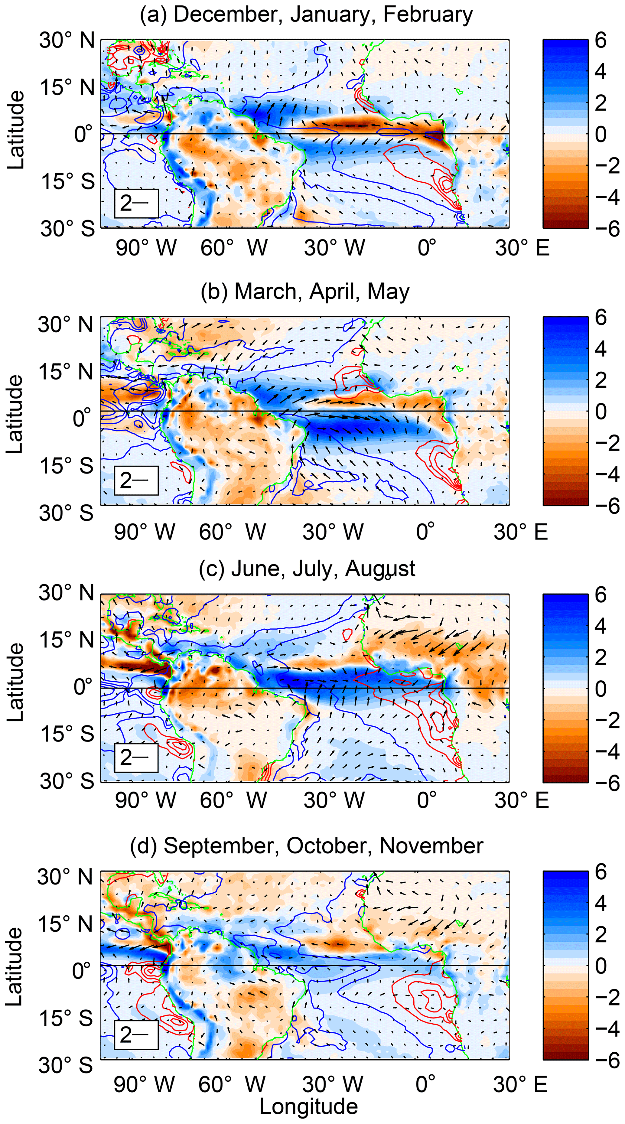
Figure 1Maps of seasonal mean biases in rainfall (filled contours), sea-surface temperature (open contours) and 10 m wind vector. Rainfall is in millimetres per day (mm d−1; see colour bar); wind vector is in metres per second (m s−1; see legend for scale) and sea-surface temperature contours are in 0.5 ∘C increments on each side of zero – red for warm biases, blue for cold biases. Biases are calculated for the seventh month of hindcast and averaged over the seasons and over the years 1998 to 2009 for coupled model S4.
There is also a seasonal cycle in the wind biases in the tropical Atlantic. The climatological winds here are easterly trade winds, and the S4 biases in autumn and winter are easterly, implying a strengthening of the trade winds. In spring, however, the bias in zonal wind turns westerly, implying a weakening of the trade winds. This “flip” of the climatological wind bias affects much of the tropical Atlantic, with the westerly bias extending from the coast of South America to the edge of the Gulf of Guinea. In summer, the westerly bias weakens with a strong convergent bias flow into the region of excess rainfall on the Equator.
Figure 2 shows the seventh-month biases in the equatorial Atlantic from month to month in more detail. Given the tendency of the bias patterns in the tropical Atlantic to be roughly zonal in structure outside the Gulf of Guinea and away from the coast of South America, the zonal mean biases are calculated in the longitude range 40–0∘ W. The transition of zonal wind bias from easterly to westerly takes place between February and April (Fig. 2c). The westerly bias dominates the tropical Atlantic through April and May before drifting northwards and weakening over the subsequent few months. Eventually, it is replaced by an easterly bias that persists for the rest of the year with varying magnitude.
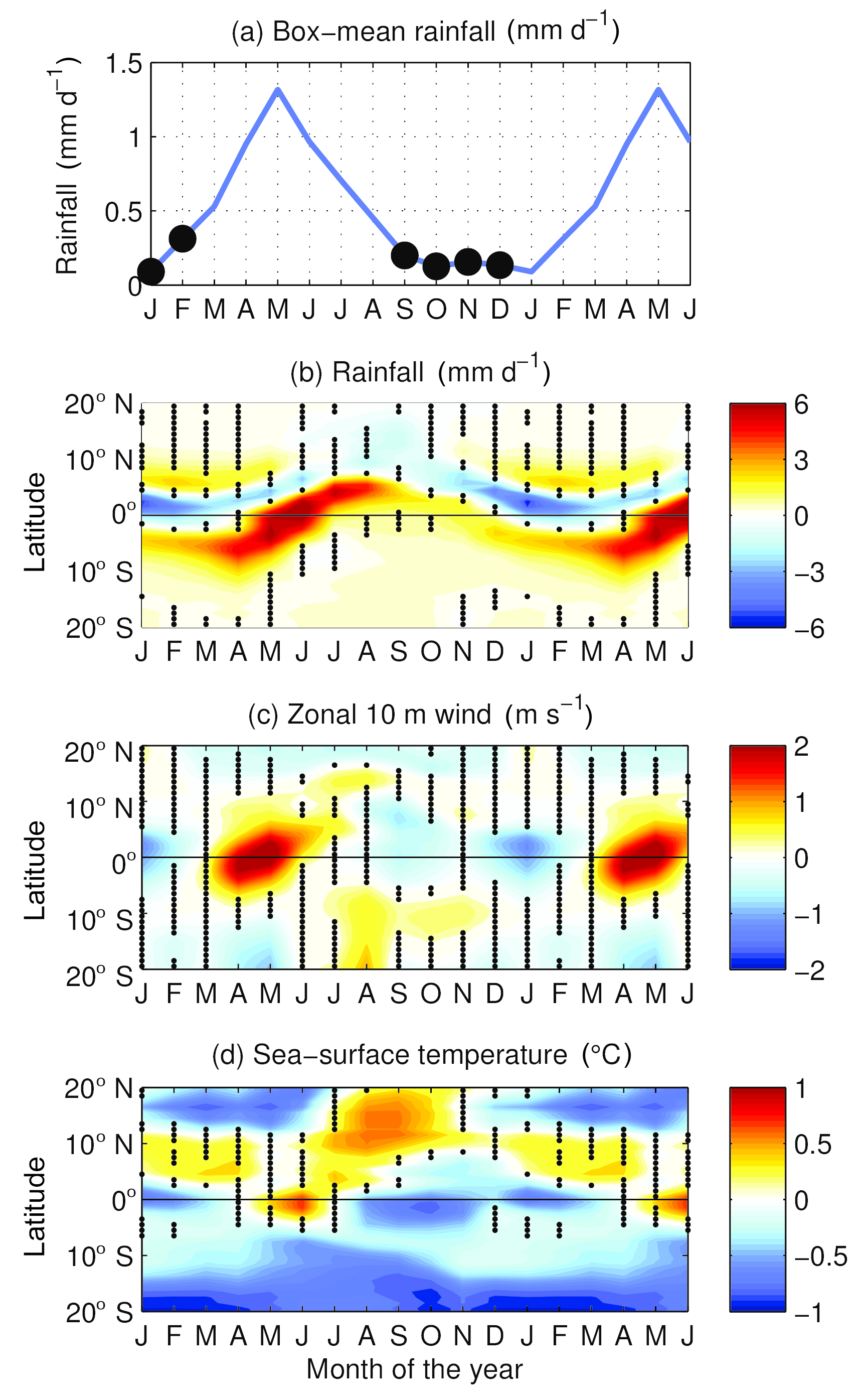
Figure 2Seasonal cycle of biases in the tropical Atlantic. All biases are calculated for the seventh month of hindcast. Panel (a) shows the bias in box-mean rainfall in the range 40–0∘ W and 20∘ N–20∘ S; the other panels show latitude–time plots of zonal mean biases in the same longitude range for (b) rainfall, (c) zonal wind at 10 m and (d) sea-surface temperature. Insignificant regions of each plot with respect to interannual variability are indicated with black spots.
An increase in rainfall bias over the tropical Atlantic occurs in the months following the onset of the westerly wind bias. Figure 2b indicates a strengthening of wet bias to the south of the Equator in April, which grows in both intensity and meridional extent to cover much of the tropical Atlantic in May and June. The result of this strengthening is an overall wet bias in rainfall in the region 20∘ S–20∘ N and 40–0∘ W (Fig. 2a). At the same time, as the equatorial wind bias becomes westerly, the cold SST bias that persists throughout most of the rest of the year (indicative of a cold tongue that is too strong) fades and eventually turns warm in April and May (Fig. 2d). In the summer, the rainfall biases decrease and the warm SST bias reverts to cold. Additionally, we see significant SST biases in the subtropics, with a cold SST bias south of the Equator that persists all year and seasonally varying biases to the north that switch between warm and cold.
The patterns of bias identified in S4 reflect patterns found in many coupled models in the tropical Atlantic (Huang et al., 2007; Richter and Xie, 2008). We can describe the springtime biases in S4 as a transition between two “bias regimes” – an easterly bias regime that exists through winter, characterised by trade winds that are too strong and cold SST biases on the Equator; and a westerly bias regime, characterised by trade winds that are too weak and warming SST biases on the Equator. We therefore focus our attention on spring, with particular attention to the transition between the two bias regimes.
3.2 Comparison of the biases in the three models
To examine the development of the equatorial bias and its relationship with biases in other aspects of the atmospheric circulation, we consider its evolution at sub-synoptic timescales. We begin by examining zonal mean quantities averaged across the central Atlantic as in Fig. 2 (longitude range 40–0∘ W) but for daily average climatologies, focussing on the first 120 d of the hindcasts initialised on 1 February. Figure 3a shows the evolution of the observed zonal mean rainfall and wind vector at 10 m for this period, during which the core of the ITCZ drifts northwards from 1 to 5∘ N. Between March and April there is a widening of the rainfall band, which extends to the south of the Equator. The winds maintain an easterly zonal component and a meridional component that is convergent towards the ITCZ.
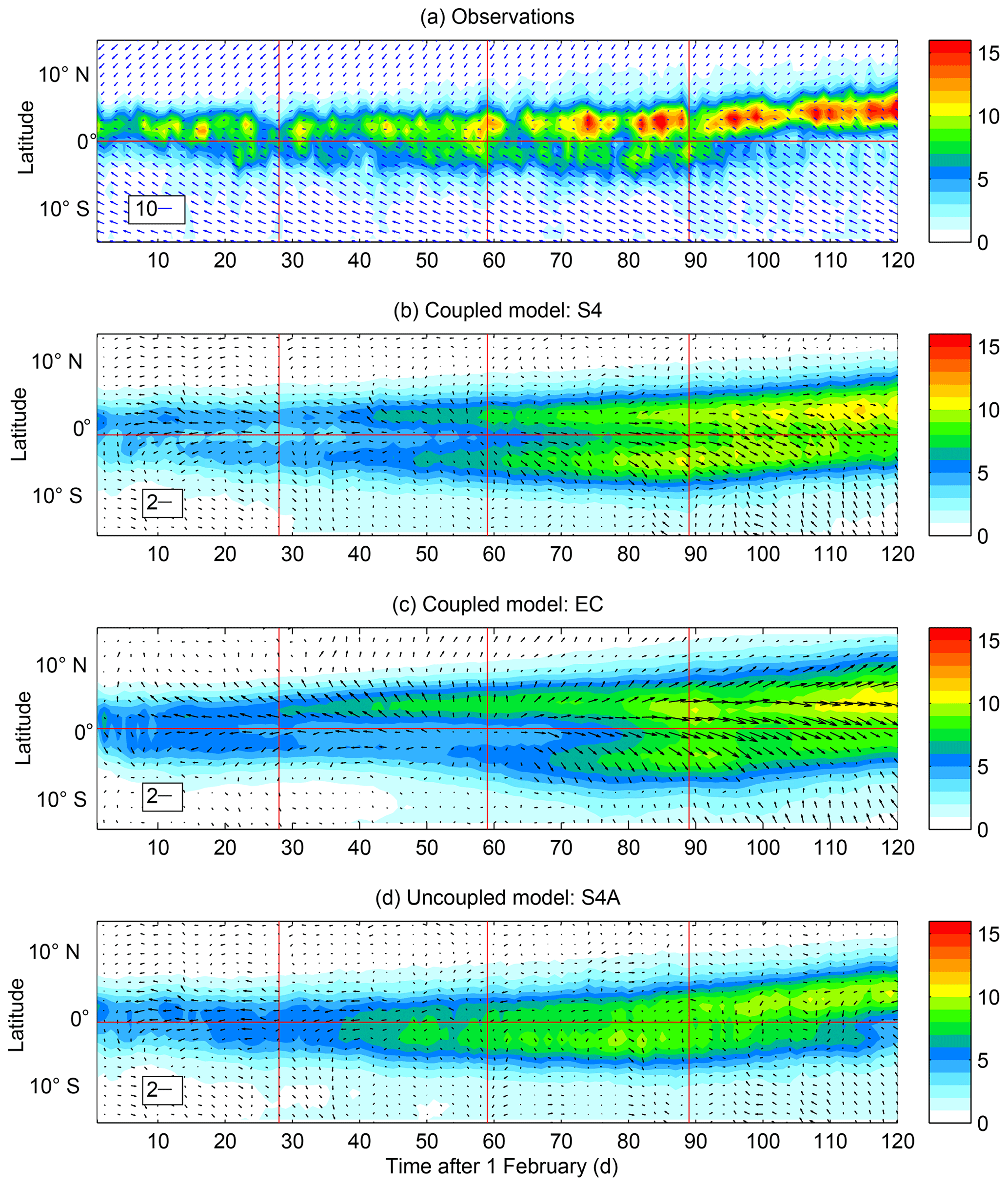
Figure 3Latitude–time plot showing the evolution of model biases, all averaged over longitudes 40–0∘ W. Panel (a) shows observed rainfall as filled contours, with observed mean vector wind at 10 m (blue arrows). Panels (b) to (d) show the rainfall according to the three models, with the wind vector biases included as black arrows. Note that the wind vectors point in the direction they would if they were on a map; the horizontal dimension here is time rather than distance. Red lines show the Equator and the boundaries between months. Rainfall is in millimetres per day (see colour bar); wind is in metres per second (see legend). Averaged over years 1996 to 2009 (S4 and S4A) and years 1981 to 2000 (EC). TRMM rainfall data in panel (a) is averaged over years 1998 to 2009.
As indicated in the previous subsection, the rainfall distribution in the S4 hindcasts takes the form of a double ITCZ (Fig. 3b). There is evidence of its development as early as mid-February, although it becomes clearer in March and April. The pre-existing northern ITCZ is displaced slightly to the north of its observed position and becomes markedly weaker, and an erroneous southern marine ITCZ develops at the same time. There is a marked strengthening of the rainfall in both ITCZ branches in April. This structure persists during May and tends to weaken towards the start of summer. The cold SST bias on the Equator also begins to develop in mid-February and then grows in late February and March in the same location as the dry region that separates the two branches of the ITCZ. The transition from a cold bias on the Equator to a warm bias begins in late March or early April, with continuous warming until the end of May (Fig. 4a).
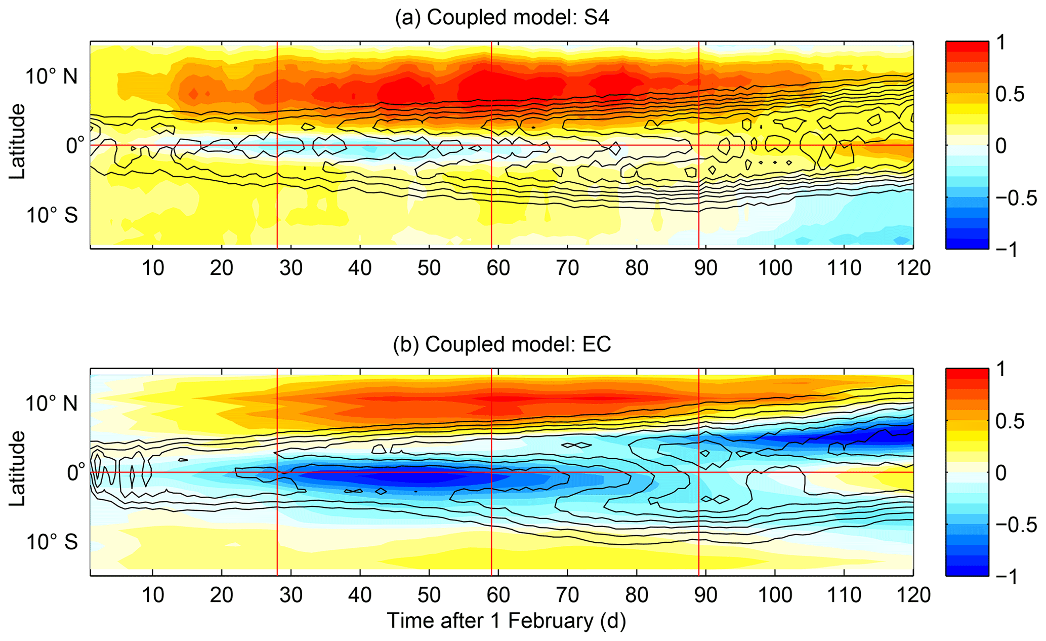
Figure 4Latitude–time plot, averaged as in Fig. 3, showing biases in sea-surface temperature in the coupled models (filled contours). The rainfall values from the models are shown here as black contours with a 1 mm d−1 interval, starting from 3 mm d−1. Sea-surface temperature biases are in degrees Celsius (∘C; see colour bar).
The initial easterly wind bias on the Equator develops within the first 10 d of hindcast (before any clear sign of a double ITCZ or a cold SST bias) and persists through February and March (Fig. 3b). The change of sign of the zonal wind bias happens around the same time the SST bias starts its transition from cold to warm and occurs more suddenly than it appears in Fig. 2. By day 50, the easterly bias has faded to near zero. In early April, the westerly biases start to grow rapidly and persist through April and May. The magnitude of this bias indicates that the trade winds on the Equator reduce to nearly calm conditions. The rapid westerly bias growth is found to occur consistently in early April when averaging over subsets of hindcast years.
Figure 5 probes the timing of this transition using hindcasts initialised at the start of March, April and May. The easterly bias regime is evident at the start of both the February and March hindcasts, although in the latter the easterly wind bias is much weaker and constrained to a narrow band north of the Equator. Accordingly, the cold SST bias is weaker, implying that the development of biases in the easterly regime has some dependence on start date and lead time. The onset of the westerly bias regime, however, occurs consistently at the start of April in the February, March and April hindcasts. Westerly biases also develop within the first few days of hindcasts initialised after the transition, as seen in the May hindcasts.
A comparison with the equatorial circulation biases in the two other models used in this study, EC and S4A, shows a similar transition between two bias regimes the equatorial circulation bias. In EC, the general evolution of bias patterns is similar to that in S4 (Figs. 3c and 4b), suggesting that relationships between the SST, rainfall and wind fields may be explained by similar mechanisms. Initially, an easterly bias develops in EC on the Equator with a developing cold SST bias and a double ITCZ structure, similar to S4. Then, the easterly wind bias becomes westerly and the cold SST bias reduces and turns warm between April and May. The rainfall in both branches of the ITCZ increases in early April, and the double ITCZ structure persists well into May.
The details of the bias patterns show both differences and commonalities. In EC, the patch of cold bias that develops in February and March is stronger and extends further south, suppressing convection south of the Equator. The result is that the southern ITCZ is weaker than the northern ITCZ in EC (in contrast to S4, where the southern ITCZ is slightly stronger) and that a fully discernible double ITCZ structure does not appear until the end of March. But the initial development of the easterly bias is similar in EC and S4, with the appearance of an easterly bias in the first 10 d that leads the development of any double ITCZ or cold SST bias, as well as a transition to westerly bias that also occurs around the start of April despite differences in the distribution of rainfall and SST bias at the time.
Another difference is the initial SST biases in the S4 and EC hindcasts. In EC, these are initially negligible, while S4 biases are already of order 0.3 ∘C by the first day. This may be a consequence of model shock (a rapid initial bias that can be caused by imbalance between the initial conditions and the model). Cycle 31R1 of the IFS, as used in EC, was used to generate ERA-Interim. Hence using this to initialise S4 (which has a more recent version of the IFS) has the potential to introduce shock (Mulholland et al., 2015; Pohlmann et al., 2017). The SST shock in S4 is of comparable magnitude to a shock found by Mulholland et al. (2015) when a model was initialised with initial conditions generated by a different version of the same model. However, these initial differences do not appear to affect the subsequent evolution of the biases in the equatorial Atlantic (Fig. 2).
Comparing S4 and S4A enables us to examine the effect of coupling on the biases. With zero SST bias effectively prescribed on the Equator, there is no suppression of convection over the Equator, and hence a clear double ITCZ bias pattern is not seen in S4A (Fig. 3d). However, the model ITCZ is still generally too broad, extends too far into the Southern Hemisphere and also increases in strength on both sides of the Equator in early April. There is evidence of a weak double ITCZ structure at times, with rainfall maxima generally located to either side of the Equator rather than on it.
As in S4, the initial easterly wind bias in S4A develops within the first 10 d – indeed, the difference in wind bias between coupled and uncoupled models in February and March is near zero despite the different rainfall pattern (Fig. 6). A full transition into westerly bias, however, does not occur in S4A. The easterly wind bias fades in late March, and the bias generally remains weak through April and May with a varying zonal component. A large effect from air–sea coupling (Fig. 6) appears with the transition between the two bias regimes.
In synthesis, both coupled models show an initial bias development consisting of an easterly bias regime. It follows a classic double ITCZ bias pattern, with excess easterly winds developing first and leading to subsequent cooling and suppression of rainfall over the Equator. The lag between wind bias growth and SST bias growth, combined with the similarity of the pattern of easterly bias across all models despite the differences in SST bias pattern, suggests that the wind bias leads the initial development of the double ITCZ pattern. The similarity of the wind bias growth between S4 and S4A implies an insensitivity to coupling that suggests that the origin of the easterly regime biases lies in the atmosphere component of the models. These results echo those of Shonk et al. (2018), who found initial easterly wind biases in the atmospheric component of S4 to be pivotal in explaining the root cause of rainfall biases in the western Pacific Ocean.
Subsequently, all three sets of hindcasts show some degree of transition away from the easterly bias regime. The transition occurs in two stages: first, a weakening of the easterly bias that is common to all three models, followed by a development of strong westerly biases that is common only to the coupled models. The seasonal nature of the transition implies an association with an aspect of the seasonal cycle of the model climatology and, for the initial reduction of the easterly bias, the most likely candidate is the systematic increase in rainfall that is common to all three models. The later intensification of the westerly bias, which is particular to the coupled models, suggests that the presence of a double ITCZ is important. The reduction of the winds suppresses the cold tongue, leading to a gradual warming of the SSTs on the Equator, allowing the development of the widespread wet bias seen in Figs. 1 and 2 through May and June.
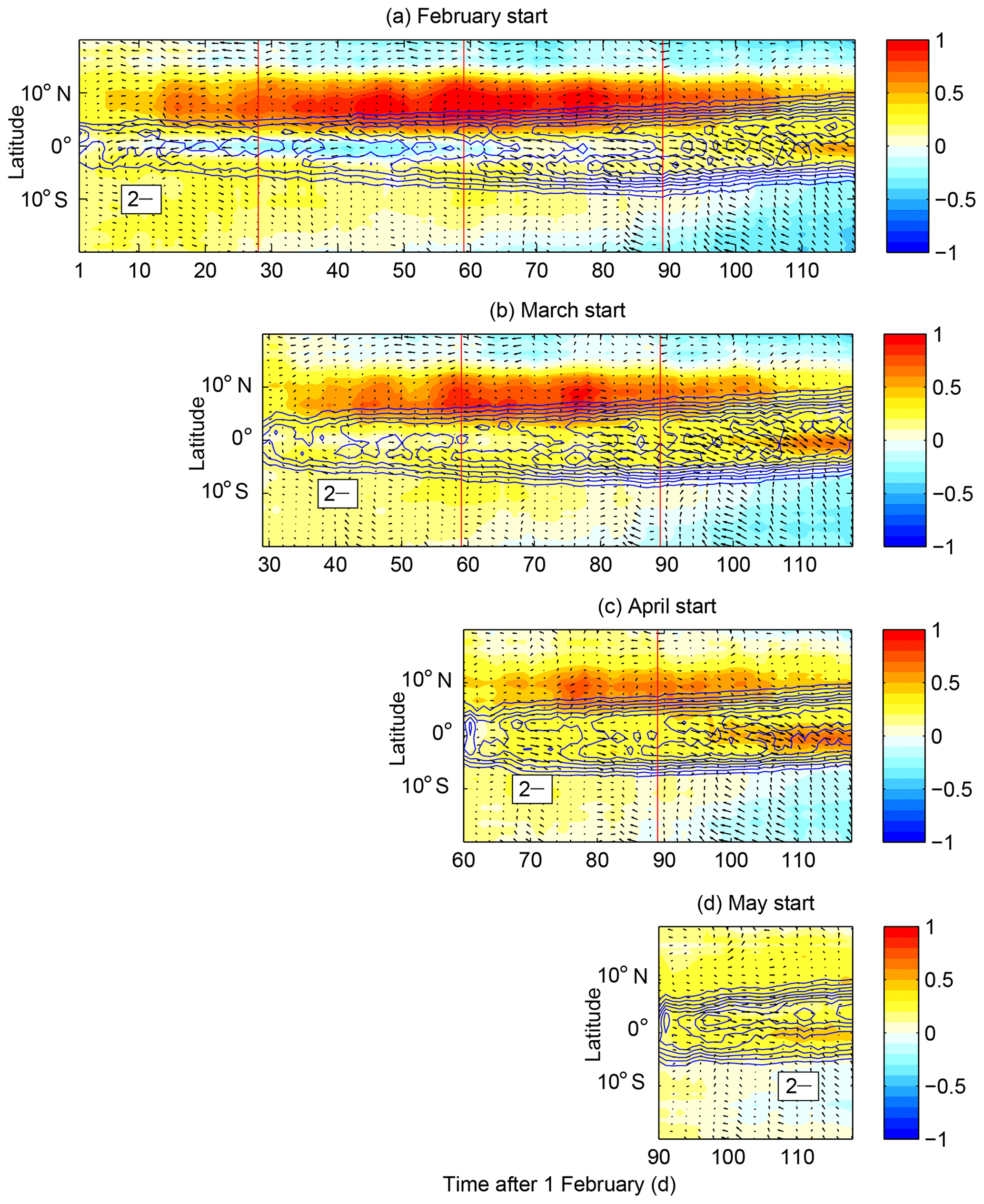
Figure 5Latitude–time plots, averaged as in Fig. 3, showing biases in sea-surface temperature (filled contours) and wind vector bias at 10 m, with contours of rainfall (in 1 mm d−1 increments from 3 mm d−1 upwards). Panel (a) shows the bias development in the S4 hindcasts starting in February; panels (b), (c) and (d) show the development in the first days of the March, April and May hindcasts. Sea-surface temperature biases are in degrees Celsius (see colour bar); winds are in metres per second (see legend).
The S4 hindcasts indicate that a pre-existing cold tongue bias is not crucial for the springtime establishment of the double ITCZ. Figure 5 shows a clear double ITCZ structure that develops rapidly in the April hindcasts despite the initial SST bias on the Equator being warm. There must be another mechanism contributing to the development of a double ITCZ, most likely associated with the coupling. We return to this point in Sect. 5.
3.3 A focus on the onset of the westerly wind bias
From the analysis in the previous subsection, it appears that the transition of the zonal wind bias in the equatorial Atlantic at the start of April is associated with two distinct bias regimes that have different associations with the rainfall. This first consists of an easterly bias, still generally associated with a double ITCZ but not obviously dependent on it; the second consists of a westerly bias that is always associated with a double ITCZ. In the following, we focus on the transition period in more detail.
Figure 7 shows model biases around the start of April, comparing dekad-mean rainfall and wind vector for the sixth to ninth dekads (10 d periods) after 1 February, a period spanning the end of March and most of April. The observed ITCZ (Fig. 7a, e, i and m) is situated a few degrees north of the Equator throughout and, over the ocean, its heaviest rainfall is generally situated over the central Atlantic. A further rainfall maximum is centred on the mouth of the Amazon, with rain falling both onto land and sea. There is also a secondary zonal band of rainfall situated just to the south of the main ITCZ that extends eastward from the coast of Brazil out to a longitude of between 30 and 20∘ W and south of the Equator.
In these dekads, two bias patterns affect the Atlantic rainfall patterns in the models: the presence of a double ITCZ, and a zonal dipole bias pattern with too much rain in the west and too little in the east. The zonal asymmetry is associated with a tendency for the model to favour marine convection over rain that is observed to fall over the coastal regions of South America. This pattern is present in all models and is particularly marked in S4A, which lacks the double ITCZ structure. In the coupled models S4 and EC, the bias patterns combine to produce a southern ITCZ with its rainfall maximum locked to the coast of South America. The distribution of the rainfall between the two ITCZ bands is different in S4 and EC, with S4 producing a stronger southern ITCZ and EC producing a stronger northern ITCZ (as seen in the previous subsection). However, in both coupled models, the southern ITCZ grows in strength through these four dekads, particularly in dekads 8 and 9.
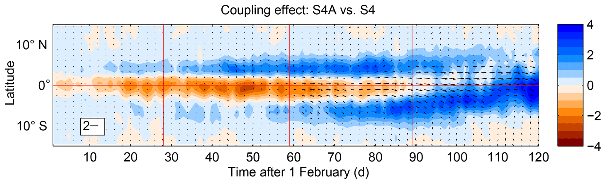
Figure 6Latitude–time plot, averaged as in Fig. 3, showing the coupling effect on rainfall (filled contours, in mm d−1) and wind vector (in m s−1).
The result of this strengthening is excess convergence off the coast of South America. Observed winds in the Atlantic consist of south-easterly trade winds across the Southern Hemisphere and north-easterly trade winds across the Northern Hemisphere that converge into the ITCZ. In the coupled models, the Southern Hemisphere trade winds are directed further south into the strengthening southern ITCZ. The location of the northern trade winds, however, remains largely unchanged, leaving a windless strip along the Equator that the trade winds do not reach. The strengthening of the rainfall in the southern ITCZ through this period corresponds with the weakening of the equatorial winds in S4 and EC (Fig. 7); from about day 60 (1 April) the winds turn westerly.
In S4A, by contrast, the weak double ITCZ structure still allows the trade winds to reach the Equator, and the equatorial winds remain easterly. Convection off the coast of South America remains active and close to the Equator. Even so, S4A does produce too much convection south of the Equator, which may still contribute to the reduction of the easterly bias at the end of March.
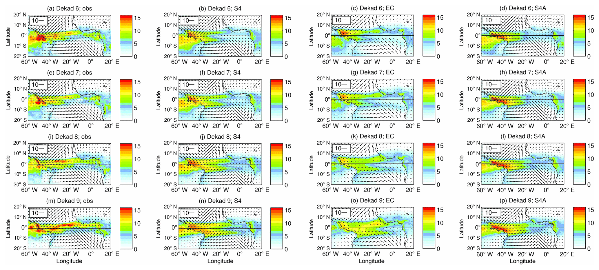
Figure 7Maps comparing rainfall and wind at 10 m in the observations and all three models. The observed panels (left column) show dekad-mean rainfall (filled contours, in mm d−1) for the sixth to ninth dekads (10 d periods) after 1 February, with wind at 10 m (in m s−1) as black arrows. The other three columns show the same for the three models, with data taken from the February hindcasts.
In summary, the onset of the westerly bias at the start of April in fact corresponds to a rapid reduction in trade wind strength from stronger than observed to very light. The common enhancement of rainfall around the start of April, in combination with the tendency of all three models to produce too much convection south of the Equator in the western Atlantic, generates excess convergence south of the Equator and redirects the trade winds. However, as the coupled models show a full double ITCZ, the Southern Hemisphere trade winds are deflected further from the Equator, leaving a zone of near-zero winds along the Equator. Hence the systematic increase in rainfall and the emergence of a double ITCZ at the start of April are crucial factors in the onset of the spring westerly wind bias.
A weak dependence on start date suggests a weak link of the ITCZ biases documented in the previous section with SST biases, or with teleconnections with other large-scale systematic biases of the model climatology (such as in the tropical Pacific; Shonk et al., 2018), which are established gradually over the course of the hindcast. The similarity in the evolution of the westerly bias over the equatorial Atlantic for different start dates (noted in Fig. 5) may therefore be taken as evidence that it is primarily due to regional processes and feedbacks with little external influence. This conclusion is supported by an analysis of the association of remote biases with those in the Atlantic.
We first considered the occurrence of propagating equatorial waves as diagnosed from the wind components at 200 hPa. Both westward and eastward waves are present in the equatorial band throughout the entire period of the February hindcasts, but there is little evidence that waves from elsewhere in the tropics are affecting the Atlantic at the time of the growth of the westerly wind bias (figures not shown).
We have already discussed local contributions to the bias pattern from rainfall biases at the coast of South America in the previous section. However, previous studies have linked large-scale biases over the land masses surrounding the Atlantic with the biases in the equatorial Atlantic. The independence of the onset of the westerly bias with start date suggests that there could be a link with an annual cycle in the regional circulation patterns. In particular, the retreat of the South American monsoon occurs typically in the middle of April (for example, Carvalho et al., 2011), and it has been proposed that the springtime equatorial Atlantic westerly wind biases are associated with a deficient South American monsoon (Richter et al., 2012).
We use diagnostics introduced by Raia and Cavalcanti (2008) to characterise the monsoon retreat. They are based on properties averaged over various Amazonian regions, designated A1 and A2 (spanning longitudes 70–50∘ W and latitudes 0–10∘ S), that are characterised by both strong monsoon rainfall and marked monsoon transitions. Figure 8 shows that the observed retreat of the monsoon here occurs around day 70. Both S4 and S4A capture the timing and the rainfall intensity of the monsoon retreat very well, while EC shows a dry bias (broadly consistent with the model's overall tendency to produce too little rainfall over land and too much over the ocean) and indicates a monsoon retreat that is about 20 d too early. Despite these differences, the transition between bias regimes in the equatorial Atlantic is very similar in timing and pattern, suggesting that the transition is not sensitive to biases over the South American continent.
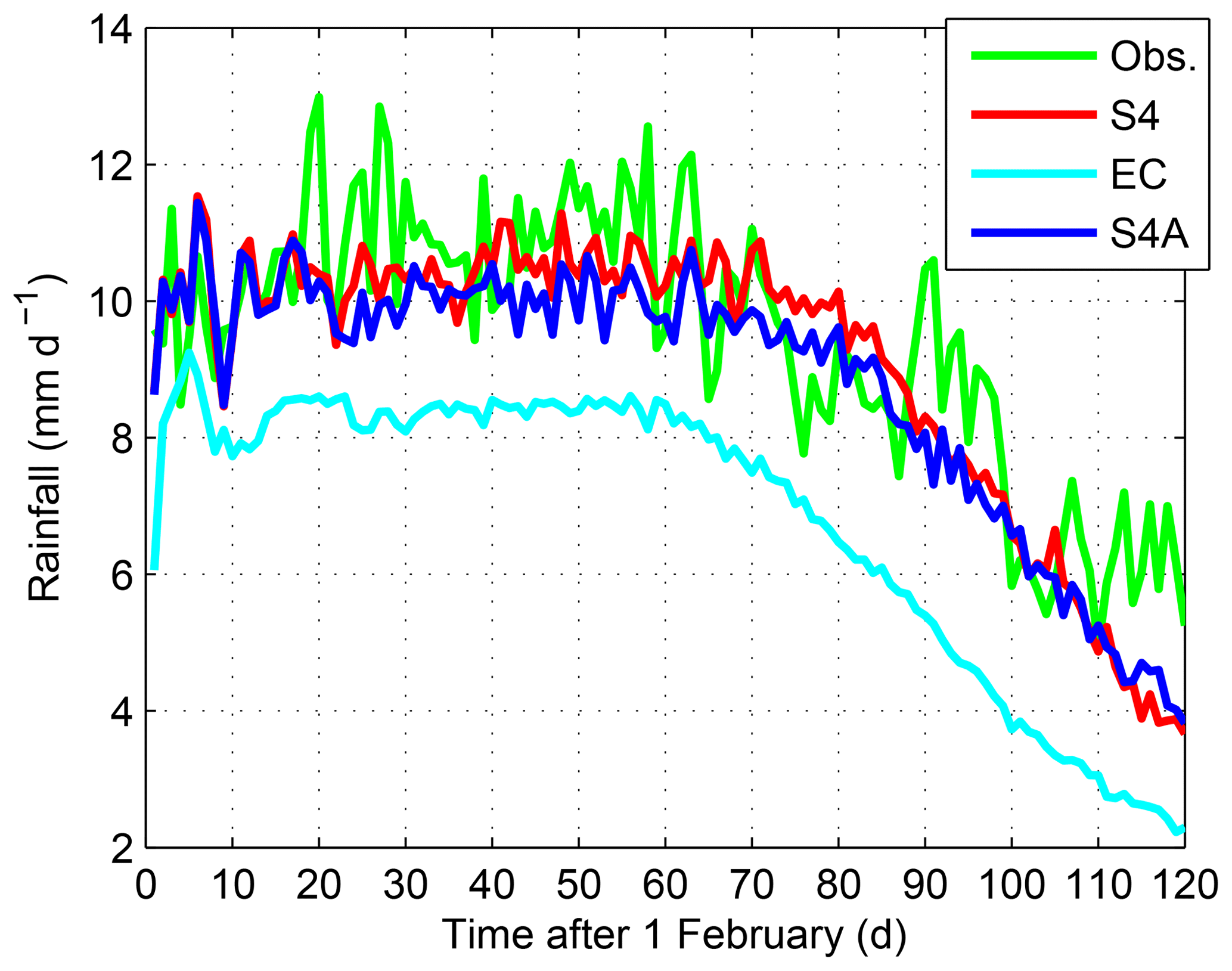
Figure 8Time series of region-mean rainfall over latitudes 0–10∘ S and longitudes 70–50∘ W, through the first 120 d of the hindcasts initialised in February. Observed (TRMM) rainfall is shown in green; the models are shown in red, blue and cyan. Full-year ranges of rainfall data are used (see caption of Fig. 3).
We finally consider the possibility for more distant teleconnections to influence the development of the equatorial biases by examining the development of local wind biases at upper levels on a dekad-by-dekad timescale. Surface wind anomalies near the Equator are often associated with vertical motion and rainfall generated by convective activity. Characteristic patterns of baroclinic motion are quickly established in response to latent heating, with a large signal aloft. Figure 9a, d and g show the coupling effect (the difference between S4 and S4A) on wind vector at 10 m and on streamfunction at 200 hPa. The first signs of the westerly bias at the surface appear in dekad 6 and grow strongly during dekad 7. The coupling effect on the streamfunction bias indicates an easterly flow aloft that develops approximately 5 to 10 d later: in dekad 7, an easterly structure starts to develop over the Equator; by dekad 8, this is well established, with a pair of anticyclones on either side of the Equator. This 10 d lag, combined with the baroclinic nature of the coupling effect, suggests that biases in convective heating are linking the circulation biases at the two levels, although the development of the lower-level biases in advance of the upper-level biases suggests that the biases affecting the circulation originate near the surface.
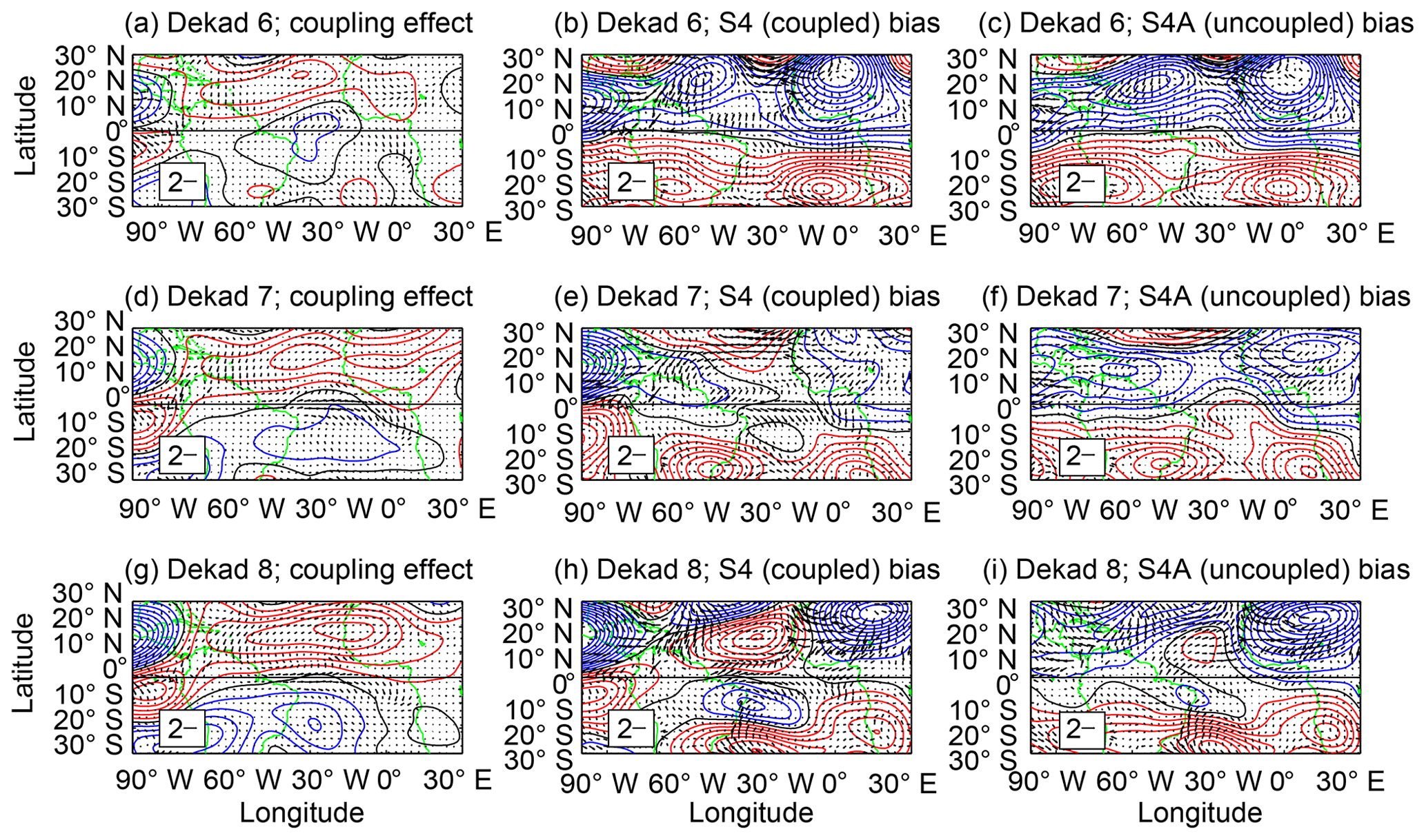
Figure 9Maps of dekad-mean biases in 10 m wind vector (black arrows, in m s−1) and 200 hPa streamfunction (contours). The middle column shows the coupled biases in S4; the right column shows the uncoupled biases in S4A; the left column shows the coupling effect (S4 minus S4A) for dekads 6 to 8. Positive streamfunction bias contours are red, negative contours are blue and the zero contour is black. North of the Equator, red contours are anticyclonic and blue contours are cyclonic. Dekads are counted from initialisation on 1 February.
The structure of the upper-level bias over the Atlantic in S4 after dekad 7 is a distinct pair of anticyclones, one on either side of the Equator, resembling a Gill–Matsuno response (Matsuno, 1966; Gill, 1980) with easterlies aloft over the Equator rather than westerlies (Fig. 9h). This implies a cooling on the Equator and hence a reduction of rainfall. The detailed circulation pattern may result from a superposition of two Gill–Matsuno patterns on either side of the Equator, associated with the double ITCZ bias. (The forcing is a band along the Equator of reduced rainfall and latent heating, flanked to the north and south by wet bands, with the southern band wetter than the northern band; the spring panel on Fig. 1 gives an idea of this distribution.) A similar bias pattern appears in S4A, also developing in dekad 7, although it is markedly weaker (Fig. 9i), which is consistent with the rainfall biases resembling a weaker version of a double ITCZ in the uncoupled model.
Based on the analysis outlined in the previous sections, our proposed chain of events for the biases in the tropical Atlantic in S4 is as follows. The model hindcasts for February and March are dominated by trade winds that are too strong, resulting in a widespread easterly bias over the ocean. Concurrently, they produce too little rainfall north of the Equator in the central Atlantic and too much rainfall in the west. The easterly wind bias is associated with a cooler ocean surface in the form of a growing cold tongue, which suppresses convection over the Equator, contributing to a double ITCZ structure. At the start of April, the wind bias changes rapidly to a westerly regime across the equatorial ocean, and zonal winds reduce in magnitude to near zero. This causes the cold tongue bias to gradually disappear and eventually the equatorial Atlantic turns warm. The elevated SSTs near the Equator enhance rainfall in the entire ITCZ with a strong zonal, double-banded structure, which only weakens toward the end of May to give rise to a single wide zonal band of rainfall.
Thus, the transition between the two bias regimes in S4 is associated with an increase in ITCZ rainfall that occurs around the start of April. This increase causes the erroneous southern ITCZ to grow, resulting in excess off-equatorial convergence that limits the northward reach of the Southern Hemisphere trade winds towards the Equator. The westerly bias therefore develops in response to the formation of a strong double ITCZ with convergence south of the Equator. We therefore turn our attention to the likely causes for the development of the springtime double ITCZ bias.
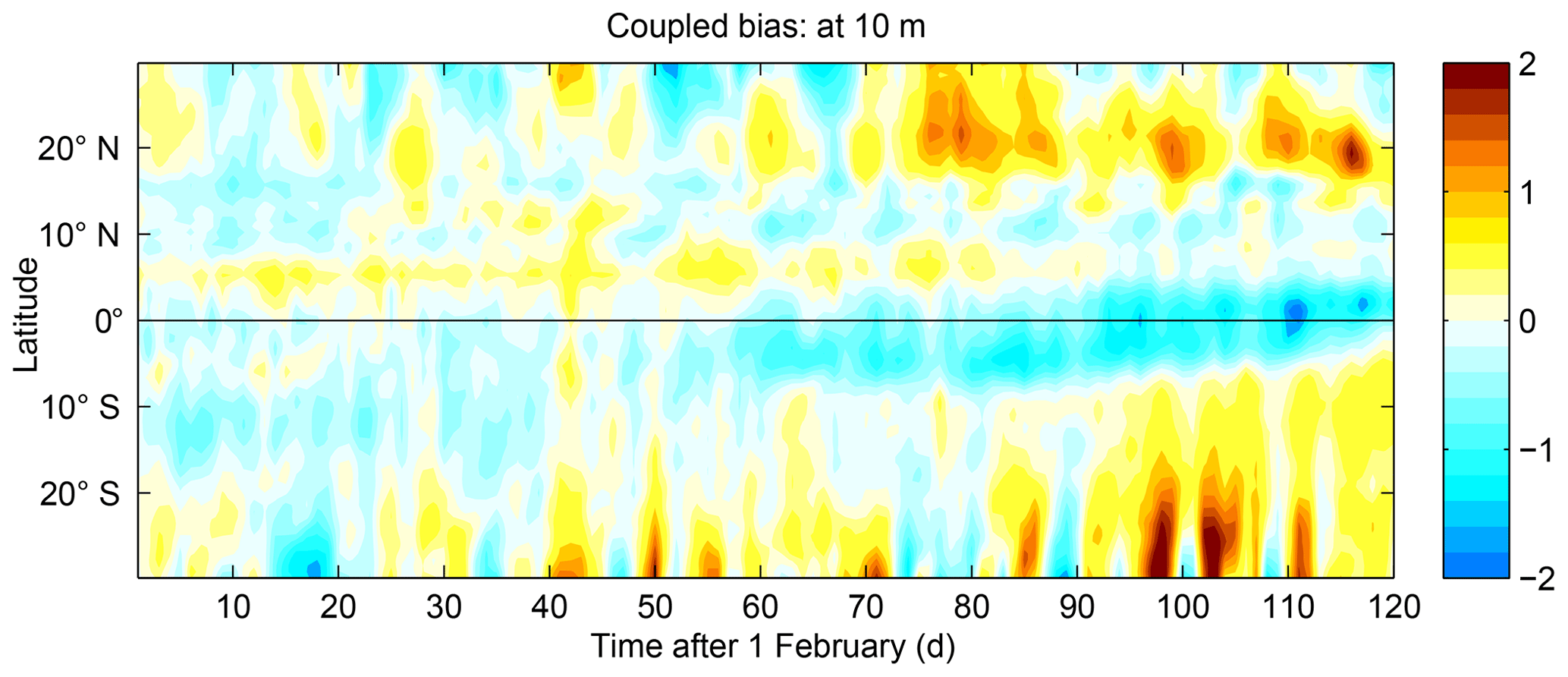
Figure 10Latitude–time plot showing the evolution of biases in meridional wind in S4 at 10 m (within the boundary layer), averaged over longitudes 20–0∘ W. Wind speeds are in metres per second and averaged over years 1996 to 2009.
The classic phenomenology of the double ITCZ bias in coupled GCMs (Lin, 2007) is associated with a cold SST bias on the Equator, and we have seen that these biases do develop at least initially in the hindcasts (Fig. 3). However, the later development of a double ITCZ in the absence of a cold SST bias (Fig. 5c) implies that there are other processes in play. A contribution could arise from the warm SST bias that develops rapidly in both coupled models between 5 and 10∘ N and persists through the bias regime transition. Such a warm bias could promote circulation changes via the mechanisms of Lindzen and Nigam (1987) and hence affect the rainfall pattern, promoting a northward shift in the northern ITCZ. However, comparison of circulation patterns in S4 and S4A in the early stages of the hindcast reveals that the changes to the circulation and rainfall associated with this warm SST bias is small with respect to the large-scale biases developing at this time. Furthermore, the strongest part of the northern ITCZ is located in the western Atlantic, while the warm SST bias is situated in the east, off the African coast. This suggests that the off-equatorial warm SST bias only provides a small contribution to the overall bias development.
Various earlier studies have considered the relationships between biases in rainfall over land and in circulation patterns over the Atlantic via sea-level pressure biases (for example, Chang et al., 2008; Richter and Xie, 2008; Richter et al., 2012). However, for the S4 model, we see little evidence of such influences. The zonal gradient of mean-sea-level pressure bias is found to be weak, and we have seen in Sect. 4 (Fig. 8) that, despite local coastal rainfall bias patterns, the effect of large-scale dry biases over the Amazon region on the bias patterns is negligible. We have also shown in Sect. 4 (Fig. 9) that the upper-tropospheric flow patterns associated with the bias regime transition in the equatorial Atlantic does not show evidence of remote origins but has the characteristics of a locally forced quasi-stationary Gill–Matsuno pattern.
Previous studies (cited above) focus on the long-term westerly biases that develop in spring rather than the specific development of the westerly bias regime we see in the seasonal hindcasts, and the processes that initiate the westerly bias at the start of April could be different to those that maintain it through the rest of spring. It may be difficult to isolate the mechanisms responsible for the initial development of the bias in equilibrated climate mode integrations. Also, the development of similar biases in different models might be dependent on different mechanisms (e.g. Toniazzo and Woolnough, 2014).
By contrast, the rapidly developing localised rainfall bias pattern seen in the hindcasts may be partly explained by errors in the model representation of low-level flow in the marine planetary boundary layer (PBL). The Equator, or more precisely the locus of vanishing vertical component of potential vorticity, presents a dynamical barrier that an adiabatic flow cannot cross (Rodwell and Hoskins, 1995). Diabatic or frictional forcing in the PBL is required to allow the flow to approach the Equator. The pressure gradient force must exceed friction effects for the flow to continue. Close to the Equator, large-scale horizontal pressure gradients in the free troposphere are weak; hence cross-equatorial flow within the PBL is driven by pressure differences arising from density gradients. The mass transport associated with this flow is strongly related to the depth of the PBL. If it is sufficiently deep, or the density gradient is strong enough, the flow can overcome the effects of surface friction and cross the Equator within the PBL. But if it is too shallow on the Equator, pure frictional potential vorticity conversion is not possible, and the flow must cross the Equator in the free troposphere, with low-level ascent in the upwind hemisphere and descent in the downwind hemisphere. This threshold behaviour of the cross-equatorial flow is described by Dvorkin and Paldor (1999) and Pauluis (2004).
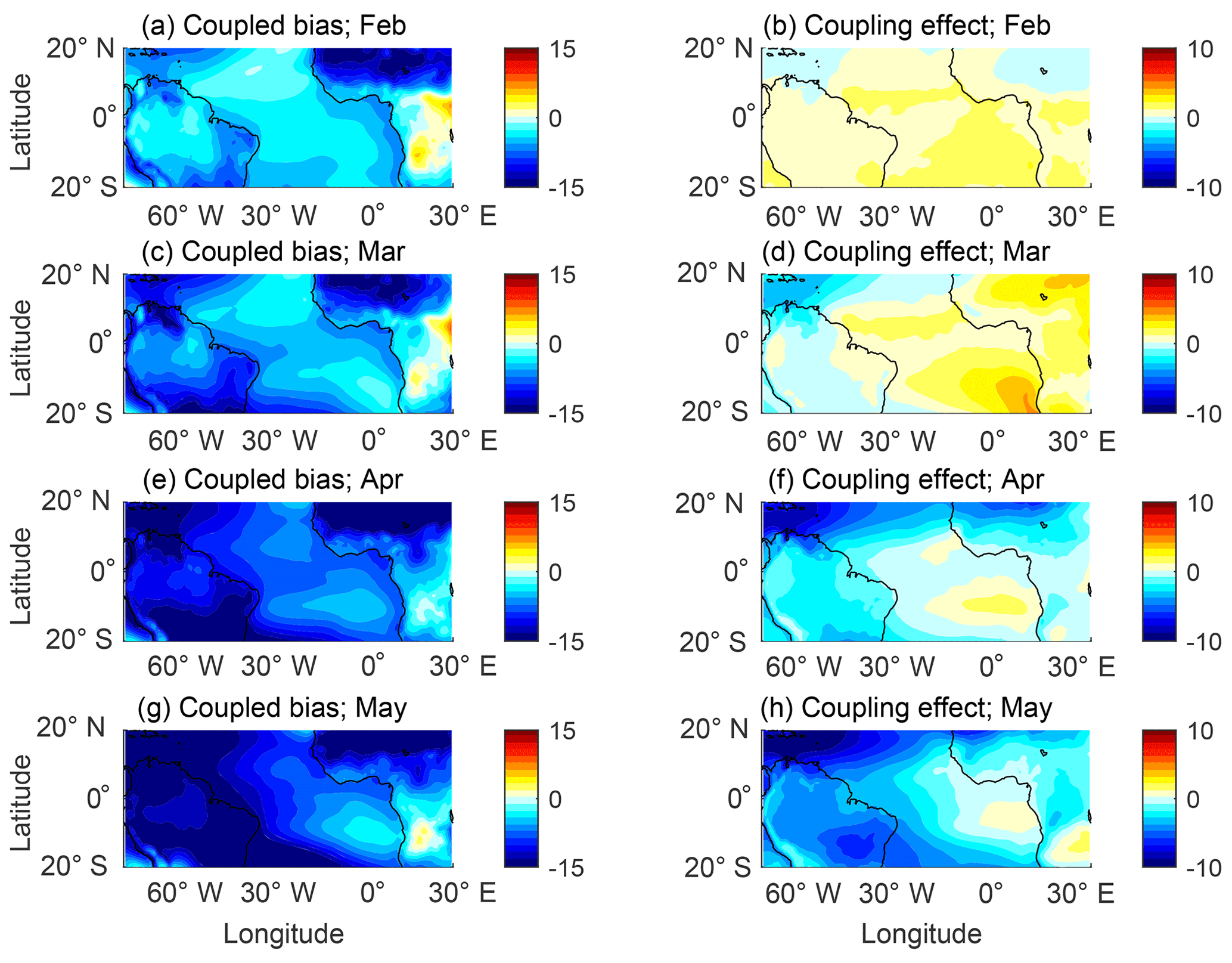
Figure 11Maps comparing geopotential thickness (in m) between models and observations. Thickness between 700 and 1000 hPa is shown. The left column shows the coupled bias in S4 with respect to ERA-Interim; the right column shows the effect of coupling on stability (S4 minus S4A). Averaged over all 14 years of hindcast and over the month in the panel titles.
The corresponding bands of ascent and descent associated with such a low-level flow pattern would, in our case, enhance and suppress convection south and north of the Equator, respectively. During the time of the transition to the westerly bias regime in S4, there is indeed a cross-equatorial southerly wind east of 20∘ W (see Fig. 7), and in this region we see suppression of the northern ITCZ (downwind) and enhancement of the southern ITCZ (upwind). Furthermore, the model shows a reduction in meridional wind at 10 m over the Equator in S4, which is consistent with the low-level flow being redirected away from the surface (Fig. 10).
The properties of the boundary layer climatologies of S4 and S4A are consistent with this hypothesis. With negligible difference in lower tropospheric stability between the two models, we may use geopotential thickness of the lower atmosphere as a proxy of boundary layer depth (increasing geopotential thickness implying decreasing boundary layer depth). In March and April, the meridional thickness gradient south of the Equator is reduced in S4 compared to S4A (see Fig. 11). This may generate meridional convergence, assuming that the difference is sufficient to cross a threshold for cross-equatorial flow in the marine boundary layer. When the boundary layer to the south of the Equator has become deep and moist enough, convection can be triggered to produce the southern ITCZ and cross-equatorial flow may proceed in the free troposphere.
Unfortunately, with the data available to us for this analysis we cannot draw a firm conclusion with regard to this hypothesis. An equally plausible origin may be found upwind of the Equator, where there are widespread cold SST biases (Fig. 2d). Increased stability here could be cooling the sea surface by suppressing the growth of trade-wind cumulus clouds and instead encouraging marine stratocumulus, which tends to reduce incoming solar radiation via its higher mean optical depth (for example, Schreier et al., 2014). Such a bias in stability could have the effect of producing a shallower boundary layer, increasing the potential for the wind to cross the Equator in the free troposphere generating the rainfall biases.
It is interesting to note that a southern ITCZ is observed to form during the spring warming season in the Pacific and Indian oceans. The Atlantic is thus an exception, in that no rainfall occurs over the ocean in a southern branch, and the model bias in this sector may be described as a failure to represent that exception. This raises the following question: what is it about the Atlantic that suppresses the southern ITCZ? The geometry of the land surrounding the basin might be an important factor. The Atlantic Ocean is much narrower than the other oceans and also much less meridional in structure (with western Africa extending far out into the basin and the north-east point of Brazil extending into the south-west Atlantic). This means that the observed heating pattern is likely to be very different. Furthermore, coastally trapped waves propagating around the African coast would travel in a westward direction along the south coast of western Africa, just north of the Equator. These waves could affect the rainfall patterns too, and any missing elements of coastal dynamics in the model could easily stall these waves in the Gulf of Guinea rather than allowing them to propagate westward along the coast into the central Atlantic.
In this study, we have used a set of seasonal hindcasts to investigate the origins of the systematic westerly wind bias that occurs on the Equator in the tropical Atlantic during spring. Fully coupled initialised hindcasts from ECMWF System 4 and EC-Earth v2.3 have been used alongside a set of hindcasts from System 4 with prescribed SSTs. The use of initialised seasonal hindcasts allows us to focus on the period when the westerly wind bias first develops and attempt to identify its root cause. In the coupled hindcasts, we found a bias regime transition from easterly wind bias to westerly wind bias that occurred rapidly at the start of April. Before the transition, in February and March, the equatorial Atlantic in the coupled models was dominated by easterly wind biases (trade winds too strong), cold SSTs and a double ITCZ, echoing similar bias patterns identified in the Pacific. Afterwards, in April and May, the trade winds reduce to near zero, leading to the reduction of the cold SST bias (which eventually turns warm) and the merging of the two branches of the double ITCZ by the end of May. The timing of the transition is not related to start date, implying that the origins of the westerly wind bias are locked to the seasonal cycle.
Despite differences in the rainfall and SST bias patterns in the two coupled models, the timing and magnitude of the transition to westerly wind bias is very similar. The strong westerly bias, however, does not develop to the same extent when the SSTs are prescribed, and neither does the development of a strong double ITCZ. This suggests that the presence of coupling and a double ITCZ are important factors in allowing the bias regime transition. We also found that the development of a double ITCZ is not driven solely by the presence of a cold SST bias on the Equator.
The increase in rainfall observed at the start of April looks to be a factor in the growth of the westerly bias. In the coupled models, excess rainfall is spread into both branches of the double ITCZ, which results in an enhancement of the erroneous southern ITCZ and generates an area of excess convergence south of the Equator. Consequently, the Southern Hemisphere trade winds that should be crossing the Equator and feeding a single northern ITCZ are redirected into this region, creating a calmer zone along the Equator where the trade winds do not reach. Furthermore, this redirection allows the southern ITCZ to strengthen while the northern ITCZ, with its Southern Hemisphere moisture source cut off, weakens.
A search for possible remote origins of the Atlantic biases has returned no strong evidence. There is no clear sign of an influence on the Atlantic from equatorial waves, and we have identified that there is no notable evidence that errors in the South American monsoon have an impact, and similarly the wind bias patterns in the upper troposphere develop in response to the surface biases rather than ahead of them. By contrast, we propose an alternative hypothesis that is consistent, even if not fully supported, by our analysis. This surmises an error in the representation of the cross-equatorial flow that is leading to erroneous ascent to the south of the Equator and descent north of the Equator, which initiates convection along an additional southern marine ITCZ branch, along with a partial suppression of the northern ITCZ. In this case, errors in the simulated thickness of the marine boundary layer would be at least a concomitant cause of the development of the springtime double ITCZ bias regime in the Atlantic. In turn, the origin of near-equatorial PBL biases may be issues with the representation of stability in the Southern Hemisphere (upwind of the Equator), possibly linked with different cloud regimes.
We recognise that there may be contributing factors to the development of the westerly bias that we have not been able to identify with the data available to us. For example, the limited availability of ocean hindcast data led to our analysis being focussed on the atmosphere. We must therefore allow the possibility that the underlying ocean conditions may contribute to the double ITCZ in the two coupled models. Even so, the rapidity of the atmospheric regime change in April and its insensitivity to the underlying SSTs and hindcast initialisation time suggest that the controlling mechanism indeed resides in the atmosphere.
While we have identified similar bias patterns in S4 and EC compared to other studies (such as Richter and Xie, 2008; Richter et al., 2012), we have found that some of the bias mechanisms are different. It is conceivable that the mechanisms that govern the development of biases in S4 and EC may not apply to other models, following the results of Toniazzo and Woolnough (2014) and Vannière et al. (2013). However, the results presented in this study should be valuable in informing future studies into the origins of biases in GCMs – for example, further work into the origins of the westerly wind bias in models other than EC and S4, or identifying more precisely the source of bias (such as issues with physics, resolution or problems with the boundary conditions) via dedicated model simulations. Tentatively, we identify as a possible target for future model development efforts in the representation of the sub-equatorial boundary layer during the transition between winter and spring circulation patterns.
The S4 and S4A data used in this study are archived on the ECMWF MARS system. They are available upon request from ECMWF (Tim Stockdale). The EC data is available upon request from the Barcelona Supercomputing Centre (Pierre-Antoine Bretonniere).
Analysis of S4 and S4A data was performed mainly by JKPS and TT; analysis of EC data was performed mainly by TDD and TT. All three authors contributed to the synthesis of the results and the preparation of the manuscript.
The authors declare that they have no conflict of interest.
We thank Tim Stockdale, Chloé Prodhomme, Steve Woolnough and Eric Guilyardi for insightful discussions. EC-Earth hindcast data were provided by the Barcelona Supercomputing Centre.
This work was performed as part of the PREFACE project, funded by European Union FP7 Environment grant agreement 603521. Later work by Jonathan K. P. Shonk was supported by Natural Environmental Research Council grant NE/N018486/1.
This paper was edited by Timothy J. Dunkerton and reviewed by two anonymous referees.
Balmaseda, M. A., Mogensen, K., and Weaver, A. T.: Evaluation of the ECMWF Ocean Reanalysis System ORAS4, Q. J. Roy. Meteorol. Soc. 139, 1132–1161. 2013.
Breugem, W. P., Chang, P., Jang, C. J., Mignot, J., and Hazeleger, W.: Barrier Layers and Tropical Atlantic SST Biases in Coupled GCMs, Tellus A, 60, 885–897, 2008.
Carvalho, L. M. V., Jones, C., Silva, A. E., Liebmann, B., and Silva Dias, P. L.: The South American Monsoon System and the 1970s Climate Transition, Int. J. Climatol., 31, 1238–1256, 2011.
Chang, C. Y., Carton, J. A., Grodsky, S. A., and Nigam, S.: Seasonal Climate of the Tropical Atlantic Sector in the NCAR Community Climate System Model 3: Error Structure and Probable Causes of Errors, J. Climate, 20, 1053–1070, 2007.
Chang, C. Y., Nigam, S., and Carton, J. A.: Origin of the Springtime Westerly Bias in Equatorial Atlantic Surface Winds in the Community Atmosphere Model Version 3 (CAM3) Simulation, J. Climate, 21, 4766–4778, 2008.
Davey, M. K., Huddleston, M., Sperber, K. R., Braconnot, P., Bryan, F., Chen, D., Colman, R. A., Cooper, C., Cubasch, U. Delecluse, P., DeWitt, D., Fairhead, L., Flato, G., Gordon, C., Hogan, T., Ji, M., Kimoto, M., Kitoh, A., Knutson, T., Latif, M., Le Treut, H., Li, T., Manabe, S., Mechoso, C., Meehl, G., Power, S., Roeckner, E., Terray, L., Vintzileos, A., Voss, R., Wang, B., Washington, W., Yoshikawa, I., Yu, J., Yukimoto, S., and Zebiak, S.: STOIC: a Study of Coupled Model Climatology and Variability in Tropical Ocean Regions, Clim. Dynam., 18, 403–420, 2002.
Dee, D. P., Uppala, S. M., Simmons, A. J., Berrisford, P., Poli, P., Kobayashi, S., Andrae, U., Balmaseda, M. A., Balsamo, G., Bauer, P., Bechtold, P., Beljaars, A. C. M., van de Berg, L., Bidlot J., Bormann, N., Delsol, C., Dragani, R., Fuentes, M., Geer, A. J., Haimberger, L., Healy, S. B., Hersbach, H., Hólm, E. V., Isaksen, L., Kållberg, P., Köhler, M., Matricardi, M., McNally, A. P., Monge‐Sanz, B. M., Morcrette, J.-J., Park, B.-K., Peubey, C., de Rosnay, P., Tavolato C., Thépaut, J.-N., and Vitart, F.: The ERA-Interim Reanalysis: Configuration and Performance of the Data Assimilation System, Q. J. Roy. Meteorol. Soc., 137, 553–597, 2011.
Dippe, T., Greatbatch, R. J., and Ding, H.: On the Relationship between Atlantic Niño Variability and Ocean Dynamics, Clim. Dynam., 51, 597–612, 2018.
Dvorkin, Y. and Paldor, N.: Analytical Considerations of Lagrangian Cross-Equatorial Flow, J. Atmos. Sci., 56, 1229–1237, 1999.
Exarchou, E., Prodhomme, C., Brodeau, L., Guemas, V., and Doblas-Reyes, F.: Origin of the Warm Eastern Tropical Atlantic SST Bias in a Climate Model, Clim. Dynam., 51, 1819–1840, 2018.
Gill, A. E.: Some Simple Solutions for Heat-Induced Tropical Circulation, Q. J. Roy. Meteorol. Soc., 106, 447–462, 1980.
Hazeleger, W., Severijns, C., Semmler, T., Ştefănescu, S., Yang, S., Wang, X., Wyser, K., Dutra, E., Baldasano, J. M., Bintanja, R., Bougeault, P., Caballero, R., Ekman, A. M. L., Christensen, J. H., van den Hurk, B., Jimenez, P., Jones, C., Kållberg, P., Koenigk, T., McGrath, R., Miranda, P., van Noije, T., Palmer, T., Parodi, J. A., Schmith, T., Selten, F., Storelvmo, T., Sterl, A., Tapamo, H., Vancoppenolle, M., Viterbo, P., and Willén, U.: EC-Earth: a Seamless Earth-System Prediction Approach in Action, B. Am. Meteor. Soc., 91, 1357–1363, 2010.
Hazeleger, W., Wang, X., Severijns, C., Ştefănescu, S., Bintanja, R., Sterl, A., Wyser, K., Semmler, T., Yang, S., van den Hurk, B., van Noije, T., van der Linden, E., and van der Wiel, K.: EC-Earth V2.2: Description and Validation of a New Seamless Earth System Prediction Model, Clim. Dynam., 11, 2611–2629, 2012.
Huang, B., Hu, Z. Z., and Jha, B.: Evolution of Model Systematic Errors in the Tropical Atlantic Basin from Coupled Climate Hindcasts, Clim. Dynam., 28, 661–682, 2007.
Hulme, M., Doherty, R., Ngara, T., New, M., and Lister, D.: African climate change: 1900—2100, Clim. Res., 17, 145–168, 2001.
Klein, S. A., Zhang, Y., Zelinka, M. D., Pincus, R. N., Boyle, J. S., and Gleckler, P. J.: Are Climate Model Simulations of Clouds Improving? An Evaluation Using the ISCCP Simulator, J. Geophys. Res.-Atmos., 118, 1329–1342, 2013.
Kummerow, C., Simpson, J., Thiele, O., Barnes, W., Chang, A. T. C., Stocker, E., Adler, R. F., Hou, A., Kakar, R., Wentz, F., Ashcroft, P., Kozu, T., Hong, Y., Okamoto, K., Iguchi, T., Kuroiwa, H., Im, E., Haddad, Z., Huffman, G., Ferrier, B., Olson, W. S., Zipser, E., Smith, E. A., Wilheit, T. T., North, G., Krishnamurti, T., and Nakamura, K.: The Status of the Tropical Rainfall Measuring Mission (TRMM) after Two Years in Orbit, J. Appl. Meteorol., 39, 1965–1982, 2000.
Lin, J. L.: The Double ITCZ Problem in IPCC AR4 Coupled GCMs: Ocean–Atmosphere Feedback Analysis, J. Climate, 20, 4497–4525, 2007.
Lindzen, R. S. and Nigam, S.: On the Role of Sea-Surface Temperature Gradients in Forcing Low-Level Winds and Convergence in the Tropics, J. Atmos. Sci., 44, 2418–2436, 1987.
Madec, G.: NEMO Reference Manual, Ocean Dynamics Component: NEMO-OPA Note du Pole de Modelisation 27, Institut Pierre-Simon Laplace, 2008.
Matsuno, T.: Quasi-Geostrophic Motions in the Equatorial Area, J. Meteorol. Soc. Jpn., 44, 25–43, 1966.
Molteni, F., Stockdale, T., Balmaseda, M., Balsamo, G., Buizza, R., Ferranti, L., Magnusson, L., Mogensen, K., Palmer, T., and Vitart, F.: The New ECMWF Seasonal Forecast System (System 4), ECMWF Technical Memorandum #656, 2011.
Mulholland, D. P., Laloyaux, P., Haines, K., and Balmaseda, M. A.: Origin and Impact of Initialisation Shocks in Coupled Atmosphere–Ocean Forecasts, Mon. Weather Rev., 143, 4631–4644, 2015.
Pauluis, O.: Boundary Layer Dynamics and Cross-Equatorial Hadley Circulation, J. Atmos. Sci., 61, 1161–1173, 2004.
Pohlmann, H., Kröger, J., Greatbatch, R. J., and Müller, W. A.: Initialisation Shock in Decadal Hindcasts due to Errors in Wind Stress over the Tropical Pacific, Clim. Dynam., 49, 2685–2693, 2017.
Raia, A. and Cavalcanti, I. F. D. A.: The Life Cycle of the South American Monsoon, J. Climate, 21, 6227–6246, 2008.
Reynolds, R. W., Rayner, N. A., Smith, T. M., Stokes, D. C., and Wang, W.: An Improved In-Situ and Satellite SST Analysis for Climate, J. Climate., 15, 1609–1625, 2002.
Richter, I. and Xie, S. P.: On the Origin of Equatorial Atlantic Biases in Coupled General Circulation Models, Clim. Dynam., 31, 587–598, 2008.
Richter, I., Xie, S. P., Wittenberg, A. T., and Masumoto, Y.: Tropical Atlantic Biases and Their Relation to Surface Wind Stress and Terrestrial Precipitation, Clim. Dynam., 38, 985–1001, 2012.
Richter, I., Xie, S. P., Behera, S. K., Doi, T., and Masumoto, Y.: Equatorial Atlantic Variability and Its Relation to Mean State Biases in CMIP5, Clim. Dynam., 42, 171–188, 2014.
Rodwell, M. J. and Hoskins, B. J.: A Model of the Asian Summer Monsoon. Part II: Cross-Equatorial Flow and PV Behaviour, J. Atmos. Sci., 52, 1341–1356, 1995.
Schreier, M. M., Kahn, B. H., Sušelj, K., Karlsson, J., Ou, S. C., Yue, Q., and Nasiri, S. L.: Atmospheric parameters in a subtropical cloud regime transition derived by AIRS and MODIS: observed statistical variability compared to ERA-Interim, Atmos. Chem. Phys., 14, 3573–3587, https://doi.org/10.5194/acp-14-3573-2014, 2014.
Seo, H., Jochum, M., Murtugudde, R., and Miller, A. J.: Effect of Mesoscale Variability on the Mean State of Tropical Atlantic Climate, Geophys. Res. Lett., 33, L09606, https://doi.org/10.1029/2005GL025651, 2006.
Shonk, J. K. P., Guilyardi, E., Toniazzo, T., Woolnough, S. J., and Stockdale, T.: Identifying Causes of Western Pacific ITCZ Drift in ECMWF System 4 Hindcasts, Clim. Dynam., 50, 939–954, 2018.
Solomon, S. D., Qin, D., Manning, M., Chen, Z., Marquis, M., Averyt, K. B., Tignor, M., and Miller, H. L. (Eds.): Contribution of Working Group I to the Fourth Assessment Report of the Intergovernmental Panel on Climate Change, Cambridge University Press, Cambridge, 2007.
Toniazzo, T. and Woolnough, S.: Development of Warm SST Errors in the Southern Tropical Atlantic in CMIP5 Decadal Hindcasts, Clim. Dynam., 43, 2889–2913, 2014.
Valcke, S.: The OASIS3 coupler: a European climate modelling community software, Geosci. Model Dev., 6, 373–388, https://doi.org/10.5194/gmd-6-373-2013, 2013.
Vannière, B., Guilyardi, E., Madec, G., Doblas-Reyes, F. J., and Woolnough, S. J.: Using Seasonal Hindcasts to Understand the Origin of the Equatorial Cold Tongue Bias in CGCMs and Its Impact on ENSO, Clim. Dynam., 40, 963—981, 2013.
Voldoire, A., Claudon, M., Caniaux, G., Giordani, H., and Roehrig, R.: Are Atmospheric Biases Responsible for the Tropical Atlantic SST Biases in the CNRM-CM5 Coupled Model?, Clim. Dynam., 43, 2963–2984, 2014.
Voldoire, A., Exarchou, E., Sanchez-Gomez, E., Demissie, T., Deppenmeier, A., Frauen, C., Goubanova, K., Hazeleger, W., Keenlyside, N., Koseki, S., Prodhomme, C., Shonk, J. K. P., Toniazzo, T., and Traoré, A.: Role of Wind Stress in Driving SST Biases in the Tropical Atlantic, Clim. Dynam., 53, 3481–3504, 2019.
Wahl, S., Latif, M., Park, W., and Keenlyside, N.: On the Tropical Atlantic SST Warm Bias in the Kiel Climate Model, Clim. Dynam., 36, 891–906, 2011.
- Abstract
- Introduction
- Approach and method
- Model biases in the tropical Atlantic
- Relationships with other model biases
- Discussion: mechanisms of bias development
- Summary and conclusions
- Data availability
- Author contributions
- Competing interests
- Acknowledgements
- Financial support
- Review statement
- References