Assessing the impact of clean air action on air quality trends in Beijing using a machine learning technique

A 5-year Clean Air Action Plan was implemented in 2013 to reduce air pollutant emissions and improve ambient air quality in Beijing. Assessment of this action plan is an essential part of the decision-making process to review its efficacy and to develop new policies. Both statistical and chemical transport modelling have been previously applied to assess the efficacy of this action plan. However, inherent uncertainties in these methods mean that new and independent methods are required to support the assessment process. Here, we applied a machine-learning-based random forest technique to quantify the effectiveness of Beijing's action plan by decoupling the impact of meteorology on ambient air quality. Our results demonstrate that meteorological conditions have an important impact on the year-to-year variations in ambient air quality. Further analyses show that the PM_2.5 mass concentration would have broken the target of the plan (2017 annual PM_2.5<60 µg m⁻³) were it not for the meteorological conditions in winter 2017 favouring the dispersion of air pollutants. However, over the whole period (2013–2017), the primary emission controls required by the action plan have led to significant reductions in PM_2.5, PM₁₀, NO₂, SO₂, and CO from 2013 to 2017 of approximately 34 %, 24 %, 17 %, 68 %, and 33 %, respectively, after meteorological correction. The marked decrease in PM_2.5 and SO₂ is largely attributable to a reduction in coal combustion. Our results indicate that the action plan has been highly effective in reducing the primary pollution emissions and improving air quality in Beijing. The action plan offers a successful example for developing air quality policies in other regions of China and other developing countries.

1 Introduction

In recent decades, China has achieved rapid economic growth and become the world's second largest economy. However, it has paid a high price in the form of serious air pollution problems caused by the rapid industrialization and urbanization associated with its fast economic growth (Lelieveld et al., 2015; Zhang et al., 2012; Guan et al., 2016). According to the World Bank, air pollution costs China's economy USD 159 billion (∼ 9.9 % of GDP equivalent) in welfare losses and was associated with 1.6 million deaths in China in 2013 (Xia et al., 2016; World Bank and IHME, 2016). Accordingly, air pollution has been receiving much attention from both the public and policymakers in China, especially in Beijing – the capital of China with around 22 million inhabitants – which has suffered extremely high levels of air pollutants (Rohde and Muller, 2015; Guo et al., 2013; Zhu et al., 2012; Cai et al., 2017). To tackle air pollution problems, China's State Council released an action plan in 2013 which set new targets to reduce the concentration of air pollutants across China (CSC, 2013). Within the plan, a series of policies, control and action plans with a focus on Beijing–Tianjin–Hebei, the Yangtze River Delta, and the Pearl River Delta regions, were proposed. To implement the national action plan and further improve air quality, the Beijing municipal government (BMG) formulated and released the “Beijing 2013–2017 Clean Air Action Plan”, which set a target for the mean concentration of fine particles (PM_2.5, particulate matter with aerodynamic diameter less than 2.5 µm) to be below 60 µg m⁻³ by 2017 (BMG, 2013). Since then, the 5-year period of 2013–2017 has seen the implementation of numerous regulations and policies in Beijing.

It is of great interest to the government, policymakers, and the general public to know whether the action plan is working to meet the set targets. Research in this area is often termed an air quality accountability study (HEI, 2003; Henneman et al., 2017a; Cheng et al., 2019). This is highly challenging because both the actions taken to reduce the air pollutants and the meteorological conditions affect the air quality levels during a particular period (Henneman et al., 2017b; Cheng et al., 2019; Liu et al., 2017; Grange et al., 2018; Chen et al., 2019). Therefore, it is essential to decouple the meteorological impact from ambient air quality data to see the real benefits in air quality by different actions.

Chemical transport models are used widely to evaluate the response of air quality to emission control policies (Wang et al., 2014; Daskalakis et al., 2016; Souri et al., 2016; Chen et al., 2019). However, there are major uncertainties in emission inventories and in the models themselves, which inevitably affect the outputs of chemical transport models (Li et al., 2017; Gao et al., 2018). Statistical analysis of ambient air quality data is another commonly used method to decouple the meteorological effects on air quality (Henneman et al., 2017b; Liang et al., 2015), including the Kolmogorov–Zurbenko (KZ) filter model and deep neural networks (Wise and Comrie, 2005; Comrie, 1997; Eskridge et al., 1997; Hogrefe et al., 2003; Gardner and Dorling, 2001). Among these models, the deep neural network models showed a better performance (i.e., higher correlation coefficient, lower root-mean-square error – RMSE) but did not allow us to investigate the effect of input variables (therefore it is referred to as a “black-box” model) (Gardner and Dorling, 2001; Henneman et al., 2015). More recently, new approaches based on regression decision trees are being developed, which are suitable for air quality weather detrending, including the boosted regression tree (BRT) and random forest (RF) algorithms (Carslaw and Taylor, 2009; Grange et al., 2018). These machine-learning-based techniques have a better performance than the traditional statistical and air quality models by reducing variance/bias and error in highly dimensional data sets (Grange et al., 2018). However, similar to the deep learning algorithms including neural networks, it is hard to interpret the working mechanism inside these models as well as the results. In addition, the decision tree models are prone to overfitting, especially when the number of tree nodes is large (Kotsiantis, 2013). An overfitting problem of a random forest model is checked by its ability to reproduce observations using an unseen training data set. Recently published R packages can partly explain and visualize random forest models including the importance of input variables and their interactions (Liaw and Wiener, 2018; Paluszynska, 2017).

Here, we applied a machine learning technique based upon the random forest algorithm and the latest R packages to quantify the role of meteorological conditions in air quality and thus evaluate the effectiveness of the action plan in reducing air pollution levels in Beijing. The results were compared with the latest emission inventory as well as results from previous study which used a chemical transport model – the Weather Research and Forecasting (WRF) – Community Multiscale Air Quality (CMAQ) model (Wong et al., 2012; Xiu and Pleim, 2001).

2 Materials and methods

2.1 Data sources

As part of the Atmospheric Pollution and Human Health in a Development Megacity programme (Shi et al., 2019), hourly air quality data for six key air pollutants (PM_2.5, PM₁₀, NO₂, SO₂, O₃, and CO) at the 12 national air quality monitoring stations in Beijing were collected from the China National Environmental Monitoring Network (CNEM) website – http://106.37.208.233:20035 (last access: 5 September 2019). Since air quality data are removed from the website on a daily basis, data were automatically downloaded to a local computer and combined to form the whole data set for this paper. All data are now available at https://github.com/tuanvvu/Air_Quality_Trend_Analysis (last access: 5 June 2019). These sites were classified in three categories (urban, suburban, and rural areas). The map and categories of the monitoring sites are given in Fig. S1 and Table S1. Hourly meteorological data including wind speed (ws), wind direction (wd), temperature, relative humidity (RH), and pressure recorded at Beijing International Airport were downloaded using the “worldMet” R package (Carslaw, 2017b). Monthly emissions of air pollutants were from the Multi-resolution Emission Inventory for China (http://www.meicmodel.org/, last access: 5 September 2019), and for the whole Beijing region. Data were analysed in RStudio with a series of packages, including “openair”, “normalweatherr”, and “randomForestExplainer” (Liaw and Wiener, 2018; Carslaw and Ropkins, 2012; Carslaw, 2017a; Paluszynska, 2017).

Figure 1 A diagram of long-term trend analysis model.

2.2 Random forest modelling

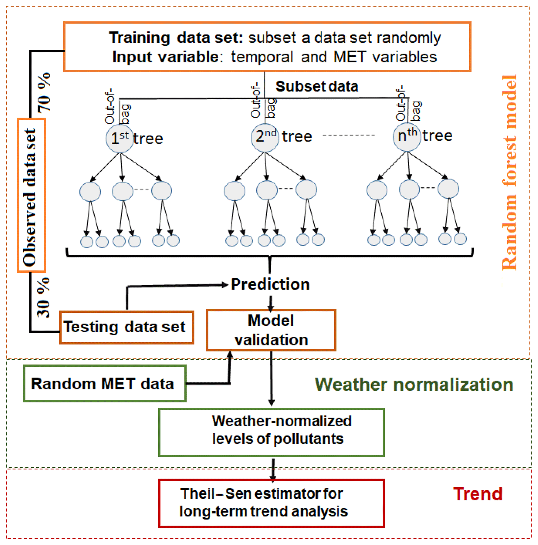
Figure 1 shows a conceptual diagram of the data modelling and analysis, which consists of three steps.

2.2.1 Building the random forest (RF) model

A decision-tree-based random forest regression model describes the relationships between hourly concentrations of an air pollutant and their predictor features (including time variables: month 1 to 12, day of the year from 1 to 365, hour of the day from 0 to 23, and meteorological parameters wind speed, wind direction, temperature, pressure, and relative humidity). The RF regression model is an ensemble model which consists of hundreds of individual decision tree models. The RF model is described in detail in Breiman (1996, 2001).

In the RF model, the bagging algorithm, which uses bootstrap aggregating, randomly samples observations and their predictor features with a replacement from a training data set. In our study, a single regression decision tree is grown in different decision rules based on the best fitting between the observed concentrations of a pollutant (response variable) and their predictor features. The predictor features are selected randomly to give the best split for each tree node. The hourly predicted concentrations of a pollutant are given by the final decision as the outcome of the weighted average of all individual decision trees. By averaging all predictions from bootstrap samples, the bagging process decreases variance, thus helping the model to minimize overfitting.

As shown in Fig. 1, the whole data sets were randomly divided into (1) a training data set to construct the random forest model and (2) a testing data set to test the model performance with unseen data sets. The training data set was comprised of 70 % of the whole data, with the rest as testing data. The RF model was constructed using R “normalweatherr” packages by Grange et al. (2018).

The original data sets contain hourly concentrations of air pollutants (response) and their predictor features that include time variables (t_trend – Unix epoch time, the day of the year, week/weekend, hour) and meteorological parameters (wind speed, wind direction, pressure, temperature, and relative humidity). These time predictor features represent effects upon concentrations of air pollutants by diurnal, weekday/weekend day, and seasonal cycles, and t_trend (Unix epoch time) represents the trend in time which captures the long-term change of air pollutant due to changes in policies/regulations, which was calculated as

$$t_{\text{trend}}={\text{year}}_i+{\displaystyle \frac{t_{\text{JD}}-\mathrm{1}}{N_i}}+{\displaystyle \frac{t_H}{\mathrm{24}{N}_i}},$$

where N_i is the number of days in a year i (the ith year from 2013 to 2017), t_H is diurnal hour time (0–23), t_JD is day of the year (1–365)) (Carslaw and Taylor, 2009).

Table S2, Fig. S3–S4, and Sect. S3 provided information on the performance of our model to reproduce observations based on a number of statistical measures including mean square error (MSE) or root-mean-square error (RMSE), correlation coefficients (r²), FAC2 (fraction of predictions with a factor of 2), MB (mean bias), MGE (mean gross error), NMB (normalized mean bias), NMGE (normalized mean gross error), COE (coefficient of efficiency), and IOA (index of agreement) as suggested in a number of recent papers (Emery et al., 2017; Henneman et al., 2017b; Dennis et al., 2010). These results confirm that the model performs very well in comparison with traditional statistical methods and air quality models (Henneman at al., 2015).

2.2.2 Weather normalization using the RF model

A weather normalization technique predicts the concentration of an air pollutant at a specific measured time point (e.g., 09:00 on 1 January 2015) with randomly selected meteorological conditions. This technique was first introduced by Grange et al. (2018). In their method, a new data set of input predictor features including time variables (day of the year, the day of the week, hour of the day, but not the Unix time variable) and meteorological parameters (wind speed, wind direction, temperature, and RH) is first generated (i.e., resampled) randomly from the original observation data set. For example, for a particular day (e.g., 1 January 2011), the model randomly selects the time variables (excluding Unix time) and weather parameters at any day from the data set of predictor features during the whole study period. This is repeated 1000 times to provide the new input data set for a particular day. The input data set is then fed to the random forest model to predict the concentration of a pollutant at a particular day (Grange et al., 2018; Grange and Carslaw, 2019). This gives a total of 1000 predicted concentrations for that day. The final concentration of that pollutant, referred to hereafter as weather normalized concentration, is calculated by averaging the 1000 predicted concentrations. This method normalizes the impact of both seasonal and weather variations. Therefore, it is unable to investigate the seasonal variation in trends for a comparison with the trend of primary emissions. For this reason, we enhanced the meteorological normalization procedure.

In our algorithm, we first generated a new input data set of predictor features, which includes original time variables and resampled weather data (wind speed, wind direction, temperature, and relative humidity). Specifically, weather variables at a specific selected hour of a particular day in the input data sets were generated by randomly selecting from the observed weather data (i.e., 1988–2017 or 2013–2017) at that particular hour of different dates within a four-week period (i.e., 2 weeks before and 2 weeks after that selected date). For example, the new input weather data at 08:00, 15 January 2015, are randomly selected from the observed data at 08:00 on any date from 1 to 29 January of any year in 1988–2017 or 2013–2017. The selection process was repeated automatically 1000 times to generate a final input data set. The 1000 data were then fed to the random forest model to predict the concentration of a pollutant. The 1000 predicted concentrations were then averaged to calculate the final weather normalized concentration for that particular hour, day, and year. This way, unlike Grange et al. (2018), we only normalize the weather conditions but not the seasonal and diurnal variations. Furthermore, we are able to resample observed weather data for a longer period (for example, 1998–2017), rather than only the study period. This new approach enables us to investigate the seasonality of weather normalized concentrations and compare them with primary emissions from inventories.

2.2.3 Quantifying long-term trend using Theil–Sen estimator

The Theil–Sen regression technique was performed on the concentrations of air pollutants after meteorological normalization to investigate the long-term trend of pollutants. The Theil–Sen approach, which computes the slopes of all possible pairs of pollutant concentrations and takes the median value, has been commonly used for long-term trend analysis over recent years. By selecting the median of the slopes, the Theil–Sen estimator tends to give us accurate confidence intervals even with non-normal data and non-constant error variance (Sen, 1968). The Theil–Sen function is provided via the “openair” package in R.

2.3 Notices, regulations, and policies for air pollution control in Beijing

The 5-year period of 2013–2017 saw the implementation of numerous regulations and policies. The “Beijing Clean Air Action Plan 2013–2017” proposed eight key regulations including (1) controlling the city development intensity, population size, vehicle ownership, and environmental resources, (2) restructuring energy by reducing coal consumption, supplying clean and green energy, and improving energy efficiency, (3) promoting public transport, implementing stricter emission standards, eliminating old vehicles and encouraging new and clean energy vehicles, (4) optimizing industrial structure by eliminating polluting capacities, closing small polluting enterprises, building eco-industrial parks and pursuing cleaner production, (5) strengthening treatment of air pollutants and tightening environmental protection standards, (6) strengthening urban management and regulation enforcement, (7) preserving the ecological environment by enhancing green coverage and water area, and (8) strengthening emergency response to heavy air pollution. We collected more than 70 major notices and policies on air pollution control from the Beijing government website (http://zhengce.beijing.gov.cn/library/, last access: 5 September 2019). Most important regulations were related to energy system restructuring and vehicle emissions (Sect. S2). These key measures include (1) reform and an upgrade action plan for coal energy conservation and emission reduction (2017), (2) “no-coal zone” for Beijing–Tianjin–Hebei in October 2017, (3) Beijing fifth phase emission standards for new light-duty gasoline vehicles (LDVs) and heavy-duty diesel vehicles (HDVs) for public transport in 2013, and (4) traffic restrictions to yellow-label and non-local vehicles to enter the city within the sixth ring road during daytime since 2015.

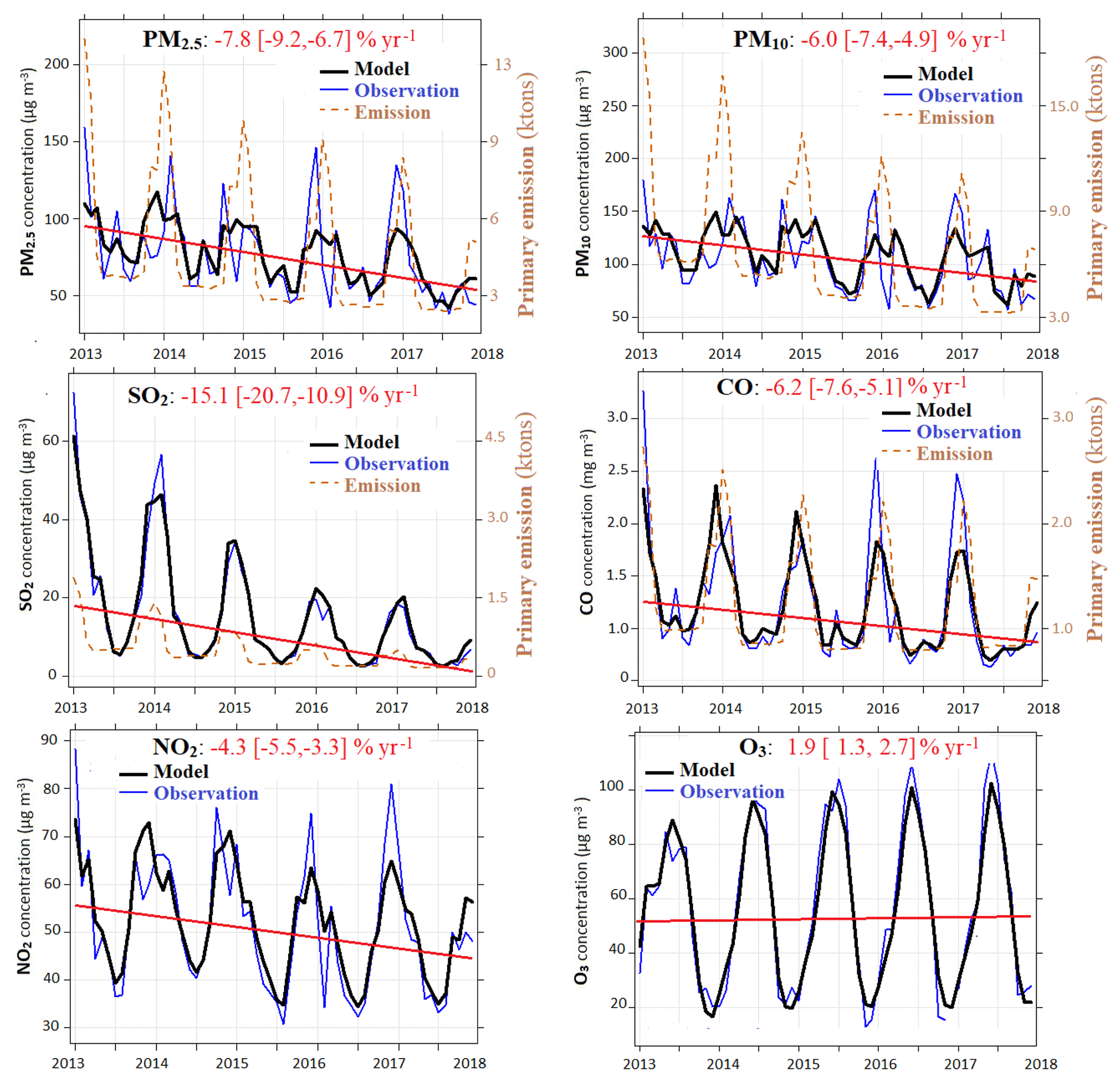
Figure 2 Air quality and primary emissions trends. Trends of monthly average air quality parameters before and after normalization of weather conditions (first vertical axis), and the primary emissions from the MEIC inventory (secondary vertical axis). “Model” in the figure means the modelled concentration of a pollutant after weather normalization. The red line shows the Theil–Sen trend after weather normalization. The black and blue dotted lines represent weather-normalized and ambient (observed) concentration of air pollutants. The red dotted line represents total primary emissions. The levels of air pollutants after removing the weather's effects decreased significantly with median slopes of 7.2, 5.0, 3.5, 2.4, and 120 µg m⁻³ year⁻¹ for PM_2.5, PM₁₀, SO₂, NO₂, and CO, respectively, while the level of O₃ slightly increased by 1.5 µg m⁻³ year⁻¹.

3 Results and discussions

3.1 Observed levels of air pollution in Beijing during 2013–2017

The annual mean concentration of PM_2.5 and PM₁₀ in Beijing measured from the 12 national air quality monitoring stations declined by 34 and 19 % from 88 and 110 µg m⁻³ in 2013 to 58 and 89 µg m⁻³ in 2017, respectively. Similarly, the annual mean levels of NO₂ and CO decreased by 16 and 33 % from 54 µg m⁻³ and 1.4 mg m⁻³ to 45 µg m⁻³ and 0.9 mg m⁻³ while the annual mean concentration of SO₂ showed a dramatic drop by 68 % from 23 µg m⁻³ in 2013 to 8.0 µg m⁻³ in 2017. Along with the decrease in annual mean concentration, the number of haze days (defined as PM_2.5>75 µg m⁻³ here) also decreased (Fig. S7). These results confirm a significant improvement of air quality and that Beijing appeared to have achieved its PM_2.5 target under the action plan (annual average PM_2.5 target for Beijing is 60 µg m⁻³ in 2017). On the other hand, the annual mean concentration of PM_2.5 is still substantially higher than China's national ambient air quality standard (NAAQS-II) of 35 µg m⁻³ (Table S3) and the WHO guideline of 10 µg m⁻³. While PM₁₀, PM_2.5, SO₂, NO₂, and CO showed a decreasing trend, the annual average concentration of O₃ increased slightly by 4.9 % from 58 µg m⁻³ in 2013 to 61 µg m⁻³ in 2017. The number of days exceeding NAAQS-II standards for O₃ 8 h averages (160 µg m⁻³) during the period 2013–2017 was 329, accounting for 18 % of total days.

3.2 Air quality trends after weather normalization

A key aspect in evaluating the effectiveness of air quality policies is to quantify separately the impact of emission reduction and meteorological conditions on air quality (Carslaw and Taylor, 2009; Henneman et al., 2017b), as these are the key factors regulating air quality. By applying a random forest algorithm, we showed the normalized air quality parameters, under the 30-year average (1988–2017) meteorological conditions (Fig. 2). The temporal variations in ambient concentrations of monthly average PM_2.5, PM₁₀, CO, and NO₂ do not show a smooth trend from 2013 to 2017 because of the spikes during pollution events. However, after the weather normalization, we can clearly see the decreasing real trend (Fig. 2). The trends of the normalized air quality parameters represent the effects of emission control and, in some cases, associated chemical processes (for example, for ozone, PM_2.5, PM₁₀). SO₂ showed a dramatic decrease while ozone increased year by year (Fig. 2). The normalized annual average levels of PM_2.5, PM₁₀, SO₂, NO₂, and CO decreased by 7.4, 7.6, 3.1, 2.5, and 94 µg m⁻³ year⁻¹, respectively, whereas the level of O₃ increased by 1.0 µg m⁻³ year⁻¹.

Table 1 A comparison of the annual average concentrations of air pollutants before and after weather normalization.

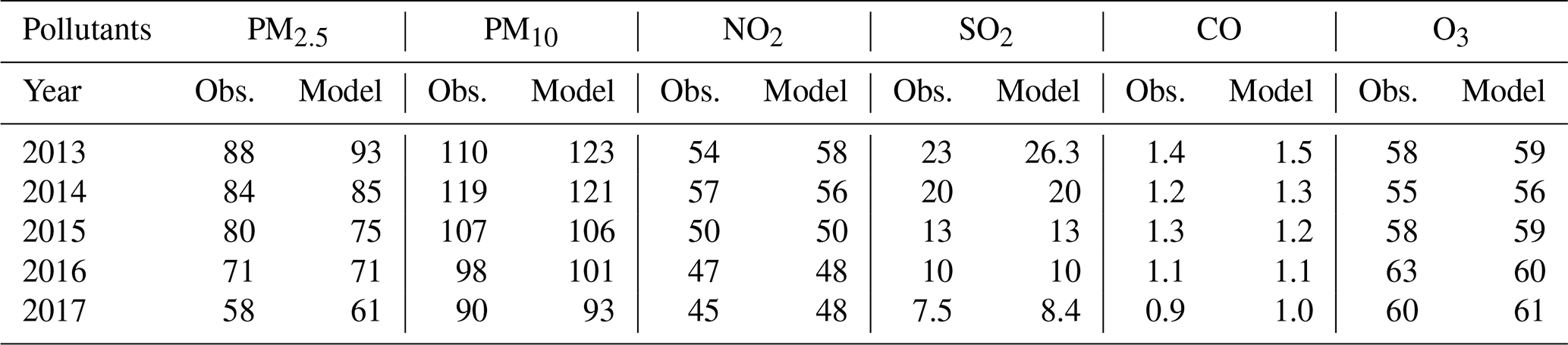
Note: Obs: observed concentration. Model.: modelled concentration of a pollutant after weather normalization. Unit: micrograms per cubic metre for all pollutants, except CO (mg m⁻³).

Table 1 compares the trends of air pollutants before and after normalization, which are largely different depending on meteorological conditions. For example, the annual average concentration of fine particles (PM_2.5) after weather normalization was 61 µg m⁻³ in 2017, which was higher than their observed level of 58 µg m⁻³ by 5.2 %. This suggests that Beijing would have missed its PM_2.5 target of 60 µg m⁻³ if not for the favourable meteorological conditions in winter 2017 and the emission reduction contributed to 10 µg m⁻³ out of the 13 µg m⁻³ (77 %) PM_2.5 reduction (71 to 58 µg m⁻³) from 2016 to 2017. Overall, the emission control led to a 34 %, 24 %, 17 %, 68 %, and 33 % reduction in normalized mass concentration of PM_2.5, PM₁₀, NO₂, SO₂, and CO, respectively, from 2013 to 2017 (Table 1).

When meteorological conditions were randomly selected from 2013 to 2017 (instead of 1998–2017) in the RF model, the normalized level of PM_2.5 in 2017 was 60 µg m⁻³, which is 1 µg m⁻³ difference to that using 1998–2017 data. This difference is due to the variation in the long-term climatology (1998–2017) to the 5-year period (2013–2017).

The observed PM_2.5 mass concentration decreased by 30 µg m⁻³ from 2013 to 2017, whereas the normalized values decreased by 32 µg m⁻³. Similarly, the observed PM₁₀ and SO₂ mass concentration decreased by 30 and 15.5 µg m⁻³ from 2013 to 2017, whereas the normalized values were 33 and 17.9 µg m⁻³. These results suggest that the effect of emission reduction would have contributed to an even better improvement in air quality (except ozone) from 2013 to 2017 if not for meteorological variations year by year.

Figure 3 Yearly change of air quality in different areas of Beijing. This figure presents yearly average changes of weather normalized air pollutant concentrations at rural, suburban, and urban sites (see Figure S1 for classification) of Beijing from 2013 to 2017. Specifically, average yearly changes are for SO₂ (−14 %, −15 %, and −16 % year⁻¹ for rural, suburban, and urban areas, respectively), CO (−9 %, −9 %, −8 % year⁻¹), PM_2.5 (−7 %, −8 %, −9 % year⁻¹), PM₁₀ (−6 %, −5 %, −7 % year⁻¹), NO₂ (−2 %, −6 %, −5 % year⁻¹), and O₃ (1 %, 0.3 %, 2 % year⁻¹). The error on the bar shows the minimum and maximum yearly change.

Figure 3 shows that the action plan has led to a major improvement in the air quality of Beijing at the urban, suburban, and rural sites, particularly for SO₂ (16 %–18 % year⁻¹), CO (8 %–9 % year⁻¹), and PM_2.5 (6-8 % year⁻¹). The action plan also led to a decrease in PM₁₀ and NO₂ but to a lesser extent than that of CO, SO₂, and PM_2.5, indicating that PM₁₀ and NO₂ were affected by other less well-controlled sources or different atmospheric processes. Urban sites showed a bigger decrease in PM_2.5, PM₁₀, and SO₂ concentrations in comparison to the rural and suburban sites (Fig. 3).

3.3 Impact of meteorological conditions on PM_2.5 levels: a comparison with results from the CMAQ-WRF model

We compared our RF modelling results with those from an independent method by Cheng et al. (2019), who evaluated the de-weathered trend by simulating the monthly average PM_2.5 mass concentrations in 2017 by the CMAQ model with meteorological conditions of 2013, 2016, and 2017 from the WRF model. The WRF-CMAQ results predict that the annual average PM_2.5 concentration of Beijing in 2017 is 61.8 and 62.4 µg m⁻³ under the 2013 and 2016 meteorological conditions, respectively, both of which are higher than the measured value – 58 µg m⁻³. Thus, the modelled results are similar to those from the machine learning technique, which gave a weather-normalized PM_2.5 mass concentration of 61 µg m⁻³ in 2017.

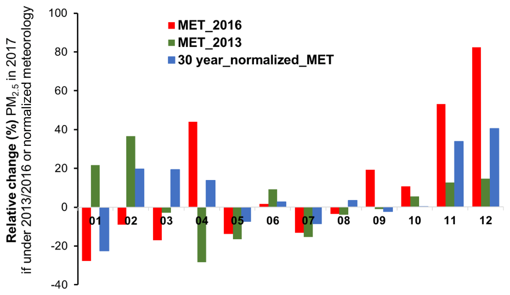
Figure 4 Relative change in monthly PM_2.5 levels in 2017 under different weather conditions. This figures presents relative changes (%) in monthly average modelled PM_2.5 concentrations in 2017 if under the 2016 (red) and 2013 (green) meteorological condition using the CMAQ model and under averaged 30 years of meteorological conditions using the machine learning technique. A positive value indicates PM_2.5 concentration would have been higher in 2017 if under the 2013 or 2016 meteorological conditions. Under the meteorological condition of 2016, monthly PM_2.5 concentration in 2017 would have been approximately 28 % lower in January but 53 % to 82 % higher in November and December. This suggests that 2017 meteorological conditions were very favourable for better air quality compared to those in 2016. If under the meteorological condition of 2013, monthly PM_2.5 concentration in 2017 would have been higher in January (22 %) and February (36 %) but only slightly higher in November (12 %) and December (14 %).

Figure 4 also shows that the PM_2.5 concentrations would have been significantly higher in November and December 2017 if under the meteorological conditions of 2016. In contrast, the PM_2.5 concentrations would have been lower in spring 2017 under the meteorological conditions of 2016 or the 30-year normalized meteorological data. The more favourable meteorological conditions in the two winter months contributed appreciably to the lower measured annual average PM_2.5 level in 2017. This also suggests that the monthly levels of PM_2.5 strongly depend upon the monthly variation in weather.

Comparison of model uncertainties from the two methods

Figure 5 compares observation and prediction of monthly concentrations of PM_2.5 by the WRF-CMAQ model and the RF model. The correlation coefficients between monthly values was 0.82, whereas that from the random forest method is > 0.99 for both the training and test data sets. The difference between the monthly observed PM_2.5 values and those simulated by the WRF-CMAQ model ranged from 3 % to 33.6 %, resulting in a 7.8 % difference in the yearly value. In contrast, the deviation between observed and predicted PM_2.5 value from the RF model ranges from 0.4 % to 7.9 % with an average of 1.5 %. In the modelled concentration of PM_2.5 from the random forest technique, standard deviation of the 1000 predicted concentrations of PM_2.5 in 2017 is only 0.35 µg m⁻³, accounting for 0.6 % of the observed PM_2.5 concentration.

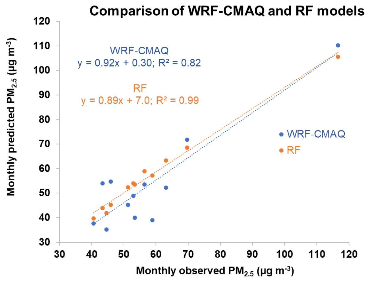
Figure 5 Comparison of predicted monthly average PM_2.5 mass concentrations by the WRF-CMAQ (Cheng et al., 2019) and RF model against observations in Beijing. WRF-CMAQ results are averaged over the whole Beijing region and the observed values refer to the average concentration of PM_2.5 over the 12 sites.

3.4 Evaluating the effectiveness of the mitigation measures in the Clean Air Action Plan

The weather-normalized air quality trend (Fig. 2) allows us to assess the effectiveness of various policy measures to improve air quality to some extent. In particular, the SO₂ normalized trend clearly shows that the peak monthly concentration in the winter months decreased from 60 µg m⁻³ in January 2013 to less than 10 µg m⁻³ in December 2017 (Fig. 2). This indicates that the control of emissions from winter-specific sources was highly successful in reducing SO₂ concentrations. The Multi-resolution Emission Inventory for China (MEIC) shows a major decrease in SO₂ emissions from heating (both industrial and centralized heating) and residential sectors (mainly coal combustion) (Fig. S8), which is consistent with the trend analyses. On the other hand, the “baseline” SO₂ concentration – defined as the minimum monthly concentration in the summer (Fig. 2) – also decreased somewhat during the same period. SO₂ in the summer mainly came from non-seasonal sources including power plants, industry, and transportation (Fig. S9). Overall, the MEIC estimated that SO₂ emissions decreased by 71 % from 2013 to 2017 (Fig. S8), which is close to the 67 % decrease in the weather-normalized concentration of SO₂ (Table 1). According to the Beijing Statistical Yearbooks (2012–2017), coal consumption in Beijing declined remarkably by 56 % in 6 years as shown in Fig. 6 (Karplus et al., 2018; BMBS, 2013–2017). The slightly faster decrease in SO₂ concentrations relative to coal consumption (Fig. S9) was attributed to the adoption of clean coal technologies that were enforced by the “Action Plan for Transformation and Upgrading of Coal Energy Conservation and Emission Reduction (2014–2020)” (Karplus et al., 2018; Chang et al., 2016). In summary, energy restructuring, e.g., replacement of coal with natural gas (Fig. 6; Sect. S2), is a highly effective measure in reducing ambient SO₂ pollution in Beijing.

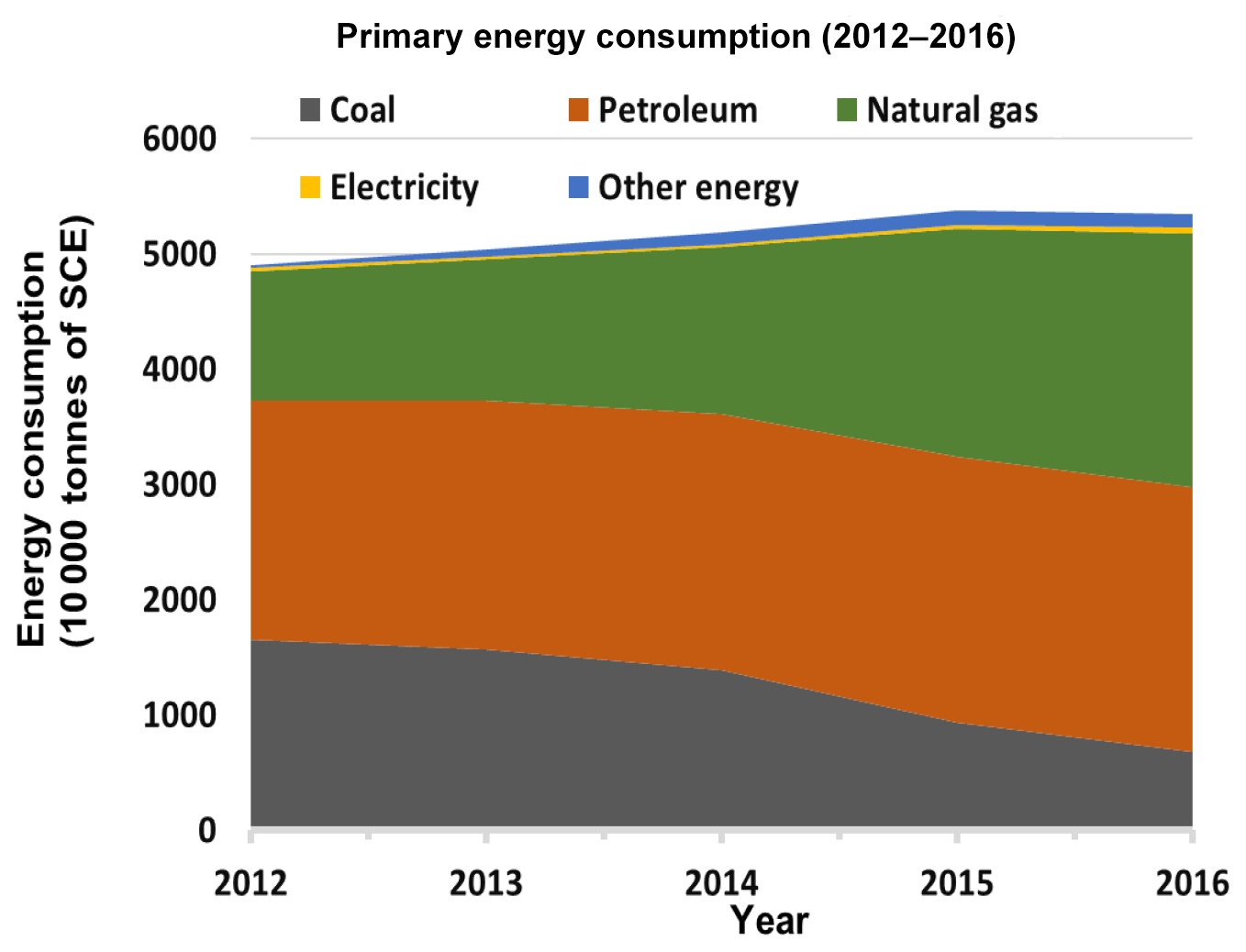
Figure 6 Primary energy consumption in Beijing. Petroleum consumption remained stable (21–23 million tonnes of coal equivalent (Mtce)) over the years while natural gas and primary electric power increased significantly by a factor of 1.8 and reached 23 Mtce in 2016. Coal consumption declined remarkably by 56.4 % from 15.7 Mtce in 2013 to 6.8 Mtce in 2016. The proportion of coal in primary energy consumption in 2016 was 9.8 %, within its target of 10 % set by the Beijing government. Note electricity here represents primary electricity.

Coal combustion is not only a major source of SO₂, but also an important source of NO_x and primary particulate matter (PM) in Beijing (Streets and Waldhoff, 2000; Zíková et al., 2016; Lu et al., 2013; Huang et al., 2014). Precursor gases including SO₂ and NO_x from coal combustion also contribute to secondary aerosol formation (Lang et al., 2017). The MEIC emission inventory showed that 8.8 %–29 % of NO_x was emitted from heating, power, and residential activities, primarily associated with coal combustion. As shown in Fig. S9, the normalized NO₂ concentration is also decreasing, but much slower than that of SO₂. Most notably, the level of SO₂ dropped rapidly in 2014 but the level of NO₂ decreased by a small proportion. The different trends between SO₂ and NO₂ indicate that other sources (e.g. traffic emissions, Fig. S9) or atmospheric processes have a greater influence on ambient concentration of NO₂ than coal combustion. For example, the chemistry of the NO–NO₂–O₃ system will tend to “buffer” changes in NO₂ causing non-linearity in NO_x−NO₂ relationships (Marr and Harley, 2002). NO₂ concentrations decreased more rapidly from January 2015, specifically by 17 %, 18 %, 10 %, and 15 % (Fig. 2) in the first 6 months of 2015, which suggests that emission control measures implemented in 2015 were effective. These measures include regulations on spark ignition light vehicles to meet the national fifth phase standard and expanded traffic restrictions to certain vehicles, including banning entry of high polluting and non-local vehicles to the city within the sixth ring road during daytime and the phasing out of 1 million old vehicles (Yang et al., 2015) (Sect. S2).

Normalized PM_2.5 decreased faster than NO₂, but more slowly than SO₂ (Fig. S9). Yearly peak normalized PM_2.5 concentrations decreased from 2013–2014 to 2015–2016 but slighted rebounded in 2016–2017. The monthly normalized peak PM_2.5 concentration decreased from 115 µg m⁻³ in January 2013 to 60 µg m⁻³ in December 2017. The biggest drop is seen in winter 2017, which decreased by more than half from the peak value in winter 2016, suggesting that the “no coal zone” policy (Sect. S2) to reduce pollutant emissions from winter-specific sources (i.e., heating and residential sectors) was highly effective in reducing PM_2.5. The normalized “baseline” concentration – minimum monthly average concentration in the summer – also decreased from 71 µg m⁻³ in summer 2013 to 42 µg m⁻³ in summer 2017. This suggests that non-heating emission sources, including industry, industrial heating, and power plants also contributed to the decrease in PM_2.5 from 2013 to 2017. These are broadly consistent with the PM_2.5 and SO₂ emission trends in MEIC (Fig. S8). A small peak in both PM_2.5 and CO in June–July seen in Fig. 2 from 2013 to 2016 attributed to agricultural burning almost disappeared over the period of the measurements and simulations in 2017, suggesting the ban on open burning is effective.

The normalized trend of PM₁₀ is similar to that of PM_2.5, except that the rate of decrease is slower. The trend agrees well with PM₁₀ primary emissions for the summer (Fig. S8). The biggest drop in peak monthly PM₁₀ concentration is seen in winter 2017, which decreased by more than half from the peak value in winter 2016, suggesting that no coal zone policy (Sect. S2) to reduce pollutant emissions from winter-specific sources (i.e., heating and residential sectors) was highly effective in reducing PM₁₀, as with PM_2.5. The rate of decrease in peak monthly PM₁₀ emission is slower than that of weather-normalized PM₁₀ concentrations, which may suggest an underestimation of the decrease by the MEIC. The normalized baseline concentration (minimum monthly average concentration, Fig. 2) – also decreased substantially from 2013 to 2017. This indicates that non-heating emission sources, including industry, industrial heating, and power plants also contributed to the decrease in PM₁₀. This is consistent with the trends in MEIC (Fig. S8). The peaks in the spring are attributed to Asian dust events.

The normalized CO trend shows that the peak CO concentration decreased by approximately 50 % from 2013 to 2017 with the largest drop from 2016 to 2017 (Fig. 2). The decreasing trend in total emission of CO in the MEIC is slower from 2015 to 2017, suggesting that CO emission in the MEIC may be overestimated in these 2 years. During 2013–2016, the CO level decreased by 26 % and 34 % for winter and summer. Similar to the normalized PM_2.5 trend, a small peak of CO concentration occurred in June–July during 2013–2016, which is likely associated with open biomass burning around the Beijing region. This peak disappeared in 2017. A major decrease in normalized CO levels in winter 2017 is mainly attributed to the no-coal zone policy (see below Sect. S2; Fig. S8).

3.5 Implications and future perspectives

We have applied a machine-learning-based model to identify the key mitigation measures contributing to the reduction of air pollutant concentrations in Beijing. However, three challenges remain. Firstly, it is not always straightforward to link a specific mitigation measure to improvement in air quality quantitatively. This is because often more than two measures were implemented on a similar timescale, making it difficult to disentangle the impacts. Secondly, we were not able to compare the calculated benefit for each mitigation measure with that intended by the government due to a lack of information about the implemented policies, for example, the start and end dates of air pollution control actions. If data on the intended benefits are known, this will further enhance the value of this type of study. Thirdly, the ozone level increased slightly during 2013–2017, especially for the summer periods (Table 1). Because ozone is a secondary pollutant, interpretation of the effects of emission changes of precursor pollutants is complex and beyond the scope of this study.

Our results confirm that the action plan has led to a major improvement in the real (normalized) air quality of Beijing (Fig. 3). However, it would have failed to meet the target for annual average PM_2.5 concentrations if not for better-than-average air pollutant dispersion (meteorological) conditions in 2017. This suggests that future target setting should consider meteorological conditions. Major challenges remain in reducing the PM_2.5 levels to below Beijing's own targets, as well as China's national air quality standard and WHO guidelines. Another challenge is to reduce the NO₂ and O₃ levels, which show little decrease or even an increase from 2013 to 2017. The lessons learned in Beijing thus far may prove beneficial to other cities as they develop their own clean air strategies.