How marine emissions of bromoform impact the remote atmosphere

It is an open question how localized elevated emissions of bromoform (CHBr₃) and other very short-lived halocarbons (VSLHs), found in coastal and upwelling regions, and low background emissions, typically found over the open ocean, impact the atmospheric VSLH distribution. In this study, we use the Lagrangian dispersion model FLEXPART to simulate atmospheric CHBr₃ resulting from assumed uniform background emissions, and from elevated emissions consistent with those derived during three tropical cruise campaigns.

The simulations demonstrate that the atmospheric CHBr₃ distributions in the uniform background emissions scenario are highly variable with high mixing ratios appearing in regions of convergence or low wind speed. This relation holds on regional and global scales.

The impact of localized elevated emissions on the atmospheric CHBr₃ distribution varies significantly from campaign to campaign. The estimated impact depends on the strength of the emissions and the meteorological conditions. In the open waters of the western Pacific and Indian oceans, localized elevated emissions only slightly increase the background concentrations of atmospheric CHBr₃, even when 1^∘ wide source regions along the cruise tracks are assumed. Near the coast, elevated emissions, including hot spots up to 100 times larger than the uniform background emissions, can be strong enough to be distinguished from the atmospheric background. However, it is not necessarily the highest hot spot emission that produces the largest enhancement, since the tug-of-war between fast advective transport and local accumulation at the time of emission is also important.

Our results demonstrate that transport variations in the atmosphere itself are sufficient to produce highly variable VSLH distributions, and elevated VSLHs in the atmosphere do not always reflect a strong localized source. Localized elevated emissions can be obliterated by the highly variable atmospheric background, even if they are orders of magnitude larger than the average open ocean emissions.

1 Introduction

Very short-lived halocarbons (VSLHs) with atmospheric lifetimes shorter than 6 months from natural oceanic sources are dominated by brominated and iodinated compounds (Carpenter and Liss, 2000; Quack et al., 2004; Law et al., 2006). VSLHs have drawn considerable interest due to their contribution to stratospheric ozone depletion and tropospheric chemistry (Solomon et al., 1994; Dvortsov et al., 1999; Salawitch et al., 2005; Feng et al., 2007; Tegtmeier et al., 2015; Hossaini et al., 2015). In this work, we focus on the VSLH bromoform (CHBr₃) since most organic oceanic bromine is released into the atmosphere in this form.

CHBr₃ concentrations measured in ocean waters are characterized by large spatial variability with elevated abundances in phytoplankton blooms (Baker et al., 2000; Liu et al., 2013) and equatorial and upwelling regions due to biological sources (Carpenter et al., 2009; Quack and Wallace, 2003; Quack et al., 2007; Fuhlbrügge et al., 2016). The open ocean generally shows homogeneous, low CHBr₃ concentrations, compared to higher concentrations and strong gradients found in coastal and shelf areas (Quack and Wallace, 2003). At the coast, high oceanic concentrations are related to macro-algae (Klick and Abrahamsson, 1992) and anthropogenic sources (Boudjellaba et al., 2016) such as power plants (Yang, 2001) and desalination facilities (Agus et al., 2009).

Due to sparse measurements and limited process understanding, existing estimates of global air–sea flux distributions of CHBr₃ and other VSLHs are subject to large uncertainties (e.g., Warwick et al., 2006; Palmer and Reason, 2009; Liang et al., 2010; Ordóñez et al., 2012; Stemmler et al., 2013; Ziska et al., 2013; Carpenter et al., 2014). The spatial and temporal distribution of elevated emissions in coastal and upwelling regions is currently based on limited observations. Campaigns in these regions suggest that emissions generally increase near coastlines, and that sporadic peak emissions with extremely high values can be found (e.g., Butler et al., 2007; Liu et al., 2013; Fuhlbrügge et al., 2016; Fiehn et al., 2017). Analysis of the measurements suggests that such peak emissions are often of limited spatial extent and cover not more than a distance of 50–100 km along the cruise track.

There are two main approaches to derive the magnitude of VSLH emissions, i.e., the “bottom-up” approach (e.g., Quack and Wallace, 2003; Carpenter and Liss, 2000; Butler et al., 2007; Ziska et al., 2013) and the “top-down” approach (e.g., Warwick et al., 2006; Liang et al., 2010; Ordóñez et al., 2012). For the bottom-up method, measured surface seawater concentrations of VSLHs at the “bottom” (surface) are extrapolated to estimate global emissions. For the top-down method, the emissions of VSLHs are constrained by the measured abundances at the “top” (atmosphere) so that model simulations based on the constrained global emission estimates reproduce the observed atmospheric concentrations. These two approaches yield different estimates of the global VSLHs emissions, with the recent top-down approaches resulting in generally higher emissions than the recent bottom-up approaches.

In the tropical ocean waters of the Atlantic and the western Pacific and Indian oceans, the existence of localized elevated CHBr₃ emissions and hot spots has been confirmed (Butler et al., 2007; Liu et al., 2013; Krüger and Quack, 2013; Fiehn et al., 2017). At the same time, these convectively active regions offer an efficient pathway for the vertical transport of short-lived oceanic compounds from the boundary layer to the stratosphere (e.g., Aschmann et al., 2009; Hossaini et al., 2012; Tegtmeier et al., 2012, 2013; Marandino et al., 2013; Liang et al., 2014). Moreover, the Asian monsoon has been recognized as an efficient transport pathway for short-lived pollutants and VSLHs (Randel et al., 2010; Hossaini et al., 2016; Fiehn et al., 2017). Given that elevated oceanic CHBr₃ emissions are expected to occur in the same regions as strong convection, it is of interest to analyze how these elevated emissions impact CHBr₃ in the atmospheric boundary layer, which feeds into the upward transport.

Measurements of CHBr₃ abundance in the atmospheric boundary layer show large spatial variability (e.g., Quack and Wallace, 2003; Montzka and Reimann, 2011; Lennartz et al., 2017). A compilation of available measurements by Ziska et al. (2013) suggests similar CHBr₃ distribution patterns in the atmospheric boundary layer as in the surface ocean, with higher mixing ratios in the equatorial, coastal, and upwelling regions. However, given the sparse base of data and the uncertainties in the spatial and temporal extent of oceanic emissions, the detailed distribution of boundary layer CHBr₃ cannot be well constrained (e.g., Hepach et al., 2014; Fuhlbrügge et al., 2013). On the one hand, the spatial and temporal extent of elevated localized emissions is usually unknown, leading to large uncertainties when estimating their overall magnitudes. On the other hand, the influence of meteorological conditions, distinctive transport patterns, and variations in atmospheric sinks, such as the background OH field (e.g., Rex et al., 2014), can be expected to modulate the effect of elevated oceanic sources. Knowledge about the interplay between sources, transport, and loss processes is relevant to understand the importance of localized elevated emissions for atmospheric abundances and to interpret existing atmospheric measurements with respect to potential sources and driving factors.

In this study, we use observational data from three tropical research cruises, one in the Indian Ocean (OASIS) and two in the western Pacific (TransBrom and SHIVA). We use the Lagrangian particle dispersion model FLEXPART to investigate the transport and atmospheric distribution of VSLHs. Taking bromoform as an example, we compare the atmospheric signals estimated from the elevated and hot spot emissions measured during the ship campaigns to the distribution derived from only uniform background emissions. We use the term “elevated emissions” when describing emissions that are on average up to a factor of 10 larger than the background and “hot spot emissions” for sporadic emissions up to a factor of 100 larger than the background. The campaigns and the FLEXPART model are introduced in Sect. 2. In Sect. 3, we discuss the distributions and variability of atmospheric CHBr₃ based on uniform background emissions. We present the observed hot spots of CHBr₃ emissions in Sect. 4.1, and compare the simulated atmospheric mixing ratios resulting from elevated emissions during three campaigns with the background values in Sect. 4.2. Conclusions are given in Sect. 5.

2 Data and methods

2.1 Background and in situ CHBr₃ emissions

In this study, we distinguish between open ocean background and in situ CHBr₃ emissions. Open ocean emissions are inferred to be around 100 pmol h⁻¹ m⁻² based on global bottom-up scenarios (Quack and Wallace, 2003; Butler et al., 2007; Liu et al., 2013; Fiehn et al., 2017; Ziska et al., 2013). While emissions for individual regions and seasons can be higher or lower than this, including negative fluxes going from the atmosphere into the ocean, 100 pmol h⁻¹ m⁻² represents a typical mean value averaged over all oceanic basins between 60^∘ S and 60^∘ N. The background open ocean emissions exclude by design emissions from coastal, shelf, and upwelling regions.

In situ oceanic emissions of CHBr₃ have been calculated from the observational data collected during three tropical ship campaigns. During each campaign, surface air and water samples were collected simultaneously at regular intervals (every 3 to 6 h). The emissions were calculated from these co-located data and the instantaneous wind speed (Ziska et al., 2013; Fuhlbrügge et al., 2016; Fiehn et al., 2017). The air–sea flux was obtained from the transfer coefficient (k_w) and the concentration gradient (Δc) between water concentration and the theoretical equilibrium water concentration (see details in Fiehn et al., 2017, and references therein):

$$\begin{array}{}\text{(1)}& F=k_{\mathrm{w}}\cdot \mathrm{\Delta }c.\end{array}$$

The two campaigns TransBrom (11–23 October 2009) and SHIVA (15–28 November 2011) took place in the western Pacific, while the OASIS campaign (11 July–6 August 2014) was conducted in the western Indian Ocean. The detailed cruise track and the magnitude of the oceanic CHBr₃ emissions of each campaign are given in Fig. 1. The in situ emissions include both open-ocean emissions and elevated emissions from coastal, shelf, and upwelling regions.

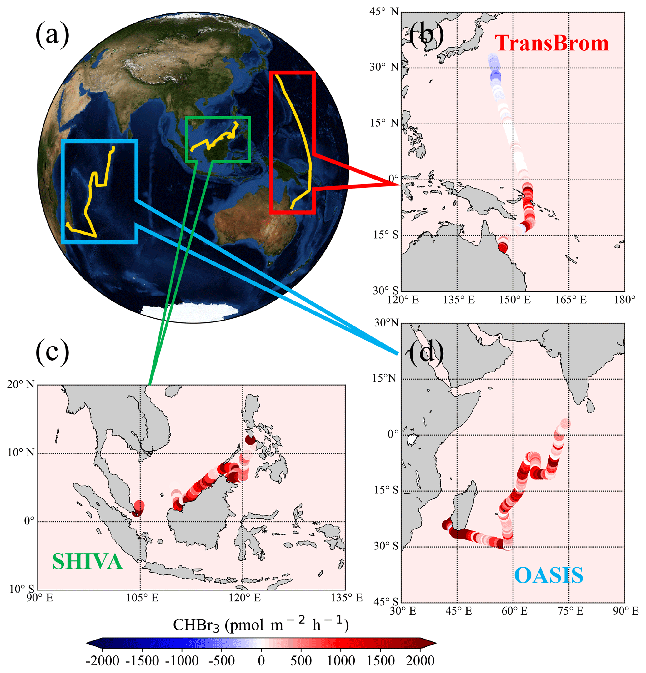
Figure 1 Cruise tracks of the three campaigns in the Indian Ocean and western Pacific (a) and CHBr₃ emissions (b, c, d) used in the model simulation. Global background emissions (100 pmol m⁻² h⁻¹) and observed emissions along the tracks of the three research cruises TransBrom (b), SHIVA (c), and OASIS (d).

2.2 Modeling

For the simulations of the atmospheric distribution and transport of CHBr₃, we used the Lagrangian particle dispersion model, FLEXPART (Stohl et al., 2005), which has been validated by previous comparisons with measurements (Stohl et al., 1998; Stohl and Trickl, 1999). Lagrangian particle models such as FLEXPART compute trajectories of a large number of so-called particles, presenting infinitesimally small air parcels, to describe the transport, diffusion, and chemical decay of tracers in the atmosphere. The model includes turbulence in the boundary layer and free troposphere (Stohl and Thomson, 1999) and a moist convection scheme (Forster et al., 2007) following the parameterization by Emanuel and Živković-Rothman (1999). The representation of convection in FLEXPART simulations has been validated with tracer experiments and ²²²Rn measurements (Forster et al., 2007). Chemical or radioactive decay of the transported tracer is accounted for by reducing the tracer mass in the air parcels according to a prescribed lifetime of the tracer. Alternatively, the loss processes can be prescribed via OH reaction based on a monthly averaged three-dimensional OH field. In this study, we employ FLEXPART version 10.0, which is driven by 3-hourly meteorological fields from ECMWF (European Centre for Medium-Range Weather Forecasts) reanalysis product ERA-Interim (Dee et al., 2011) with a horizontal resolution of $\mathrm{1}{}^{\circ }\times \mathrm{1}{}^{\circ }$ and 61 vertical model levels.

We performed two kinds of simulations based on the different emissions scenarios. The first one used the uniform global background emissions, and the second one used in situ emissions observed during individual ship campaigns. Trajectories released from the global ocean surface or along the cruise track carry the amount of CHBr₃ prescribed by the respective emissions scenario. Chemical decay of CHBr₃ was accounted for by

$$\begin{array}{}\text{(2)}& m\left(t+\mathrm{\Delta }t\right)=m\left(t\right)\exp \left(-\mathrm{\Delta }t/\mathit{\beta }\right),\end{array}$$

where m is the mass of CHBr₃ in the air parcel, $\mathit{\beta }=T_{\mathrm{1}/\mathrm{2}}/\ln \left(\mathrm{2}\right)$ is the e-folding lifetime of CHBr₃, and T_1∕2 is the half-life of CHBr₃ (Stohl et al., 2005). In our study, a half-life of 17 d (e-folding lifetime of 24 d) is prescribed for CHBr₃ during all runs (Montzka and Reimann, 2011). For the background runs, a uniform air–sea flux of 100 pmol h⁻¹ m⁻² was prescribed over all ocean surface area between 60^∘ S and 60^∘ N. Three runs were conducted covering the time period of the campaigns with a 1-month spin-up period in each case to reach a stable background concentration in the atmosphere.

For the in situ emissions of each campaign, simulations were based on the calculated CHBr₃ air–sea flux (see Fig. 8), which was released along the cruise track. The periods of the corresponding background simulations with emissions over the whole time period were the same as the campaign simulations. For each observational data point, an emission grid cell centered on the measurement location was created. These grid cells were designed to be adjacent along the cruise track and, based on the density of the measurements, were about 0.1–2.0^∘ wide in the cruise track direction. The grid cells were chosen to be of a fixed width (0.5 or 1^∘) in the other direction and thus add up to the narrow band of 0.5 or 1^∘ width centered along the cruise track (Fig. 1). Our design of the emission grid cells assumes that the elevated emissions can extend over a distance of 0.5–1^∘. This choice has been motivated by the spatial variability of the measurements along the cruise track (see also Sect. 4.1 and Fig. 7). Elevated emissions larger than 1000 pmol h⁻¹ m⁻² were found at 77 different locations along the three cruise tracks examined in this paper. Out of the 77 measurements, only 11 corresponded to singular locations with no adjacent high emissions at the neighboring points. The other 66 measurements are clustered together at 18 different locations with at least two adjacent observational points showing emissions larger than 1000 pmol h⁻¹ m⁻². We defined the length of such a location of elevated emissions as the distance between the first and last data point with an air–sea flux exceeding 1000 pmol h⁻¹ m⁻². Most of the 18 locations extended over a distance larger than 0.5^∘ (13 out of 18) and nearly half were larger than 1^∘ (8 out of 18), supporting our choice of the width of the emissions grid cells. Note that the spatial extent of the hot spots was comparable to the wind field resolution that drove our trajectory simulations. The amount of CHBr₃ released from each grid cell was determined by the observational air–sea flux of the corresponding data point and scaled with the width of the narrow emission band described above. The specified CHBr₃ emission from each cell was kept constant for the duration of the model run and distributed over a fixed number of trajectories. In order to capture the small-scale processes (e.g., convection), the 2000 trajectories were released from each $\mathrm{1}{}^{\circ }\times \mathrm{1}{}^{\circ }$ area of background runs and 20 000 from each emission grid of regional in situ runs.

Output data in the form of CHBr₃ volume mixing ratios (VMRs) available on a user-defined grid were calculated by

$$\begin{array}{}\text{(3)}& \text{VMR}=\left({\displaystyle \frac{C_{\mathrm{T}}}{{\mathit{\rho }}_{\mathrm{a}}}}\right)\cdot \left({\displaystyle \frac{m_{\mathrm{a}}}{m_{\mathrm{T}}}}\right),\end{array}$$

where C_T is the CHBr₃ mass concentration, ρ_a is the density of the air, and m_a and m_T are the molecular weight of air and CHBr₃, respectively.

For each grid cell, the CHBr₃ mass concentration is given by

$$\begin{array}{}\text{(4)}& C_{\mathrm{T}}={\displaystyle \frac{\mathrm{1}}{V}}{\sum }_{i=\mathrm{1}}^N{m}_i{f}_i,\end{array}$$

with m_i being the mass of CHBr₃ for air parcel i, f_i the mass fraction of CHBr₃ of parcel i attributed to the respective grid cell, N the total number of the air parcels, and V the volume of the grid cell (Stohl et al., 2005). We run FLEXPART in the non-domain-filling mode; therefore the parcel distribution is not correlated with air density. Air parcels, and thus bromoform, can accumulate in regions of low wind speeds where the relatively long residence time allows oceanic emissions to constantly add new parcels. Similarly, parcels can accumulate in regions of convergence where horizontal inflow pools marine boundary layer air from different regions. The output files are recorded at a horizontal resolution of $\mathrm{1}{}^{\circ }\times \mathrm{1}{}^{\circ }$ and $\mathrm{0.5}{}^{\circ }\times \mathrm{0.5}{}^{\circ }$ for background runs and in situ runs, respectively, at every 100 m from 100 m to 1 km altitude, and every 1 km from 1 to 20 km altitude every 3 h.

3 Atmospheric CHBr₃ based on open ocean background emissions

In this section, we show the impact of atmospheric transport patterns on the atmospheric CHBr₃ distribution, with the uniform background CHBr₃ emission simulations. The CHBr₃ mixing ratios in the lower atmosphere diagnosed from the uniform background emissions (referred to as CHBr₃ background mixing ratios hereinafter) vary significantly from campaign to campaign and also within each campaign region. Figures 2 to 4 present snapshots of the CHBr₃ background mixing ratios and the simultaneous wind fields from ERA-Interim for the three campaigns. For TransBrom (Fig. 2), high CHBr₃ mixing ratios appear south of 15^∘ N with a maximum near the Equator, where the wind is weak. In the northern Pacific, which is dominated by an anticyclone centered around 165^∘ E, 30^∘ N, the background values are much lower. On 10 October 2009, two bands of extremely low wind fields exist, one directly south of the Equator and one tilting from 15 to 5^∘ N, which both coincide with the highest CHBr₃ abundances. On 20 October, these two bands collided into one with the lowest winds centered around 165^∘ E, where we again find very high values of CHBr₃ of up to 0.8 ppt. For both case studies, the highest values are found in the region of the lowest wind speeds or slightly shifted towards the region of strongest wind shear. Regions of high wind speeds, such as the northern Pacific anticyclone, are characterized by very low CHBr₃.

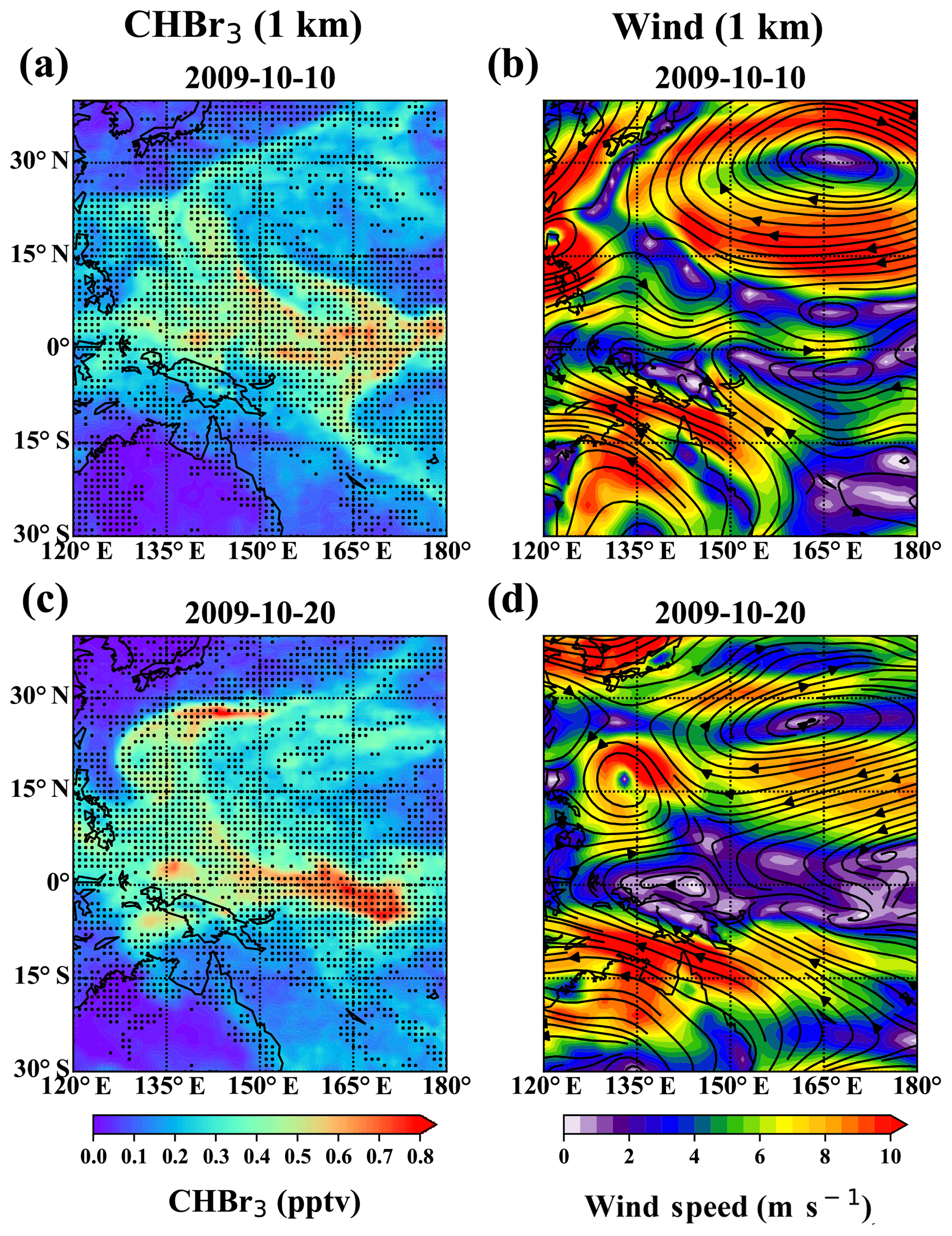
Figure 2 Two snapshots of spatial distributions of atmospheric CHBr₃, derived from uniform oceanic background emissions of 100 pmol m⁻² h⁻¹ (a, c) and ERA-Interim reanalysis wind fields (b, d) at 1 km altitude during TransBrom. The wind speed is denoted by color shades and the directions are denoted by the stream lines. The regions of convergence are shaded in (a, c).

For the SHIVA case (Fig. 3), the background CHBr₃ accumulates in a narrow region near Indonesia, with corresponding wind fields smaller than 3 m s⁻¹. North of Indonesia, the strong easterly trade winds generally above 10 m s⁻¹ prevent the accumulation of higher background values within the region. Again, the two case studies illustrate how changes of the wind patterns within a few days drive changes of the background CHBr₃ distribution. Another particular example is the northward extension of the low equatorial winds around 90^∘ E on 16 November 2011, which leads to higher CHBr₃ north of the Equator up to 15^∘ N.

Figure 3 Same as Fig. 2, but for the SHIVA case.

For OASIS (Fig. 4), the wind speed is higher than for the other two campaigns and these strong southeast/southwest trade winds associated with the Asian monsoon extend over most of the Indian Ocean. Consistent with the stronger winds, the background values for the OASIS case are significantly lower than for the other two cases, although they also show accumulations in certain regions. These relatively higher background mixing ratios appear partially in regions of low wind speeds (e.g., near the Equator between 70 and 90^∘ E on 17 July) or in adjacent regions of high wind shear (e.g., north of the Equator between 70 and 90^∘ E for both case studies). For the latter case, the CHBr₃ accumulation also extends into the region of high wind speeds, which is different from the distribution found for the TransBrom and SHIVA regions. This difference occurs because the east coast of the Indian subcontinent offshore is a region with wind convergence (dotted region), which tends to accumulate air masses therein.

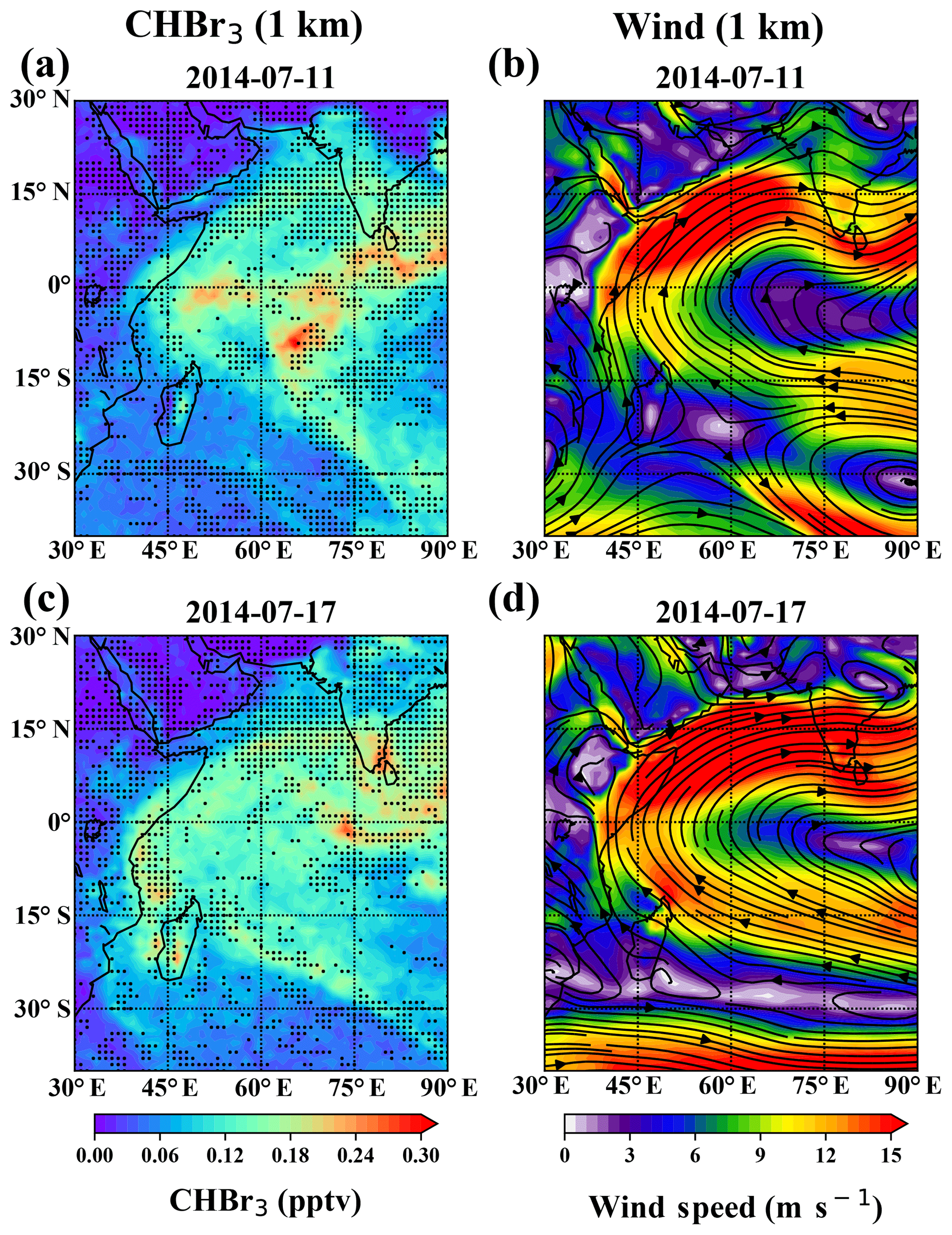
Figure 4 Same as Fig. 2, but for the OASIS case.

Given that the accumulation of CHBr₃ background mixing ratios follows the wind field patterns on a regional scale in most cases, we hypothesize that the interplay between wind speed and convergence may influence the CHBr₃ distribution.

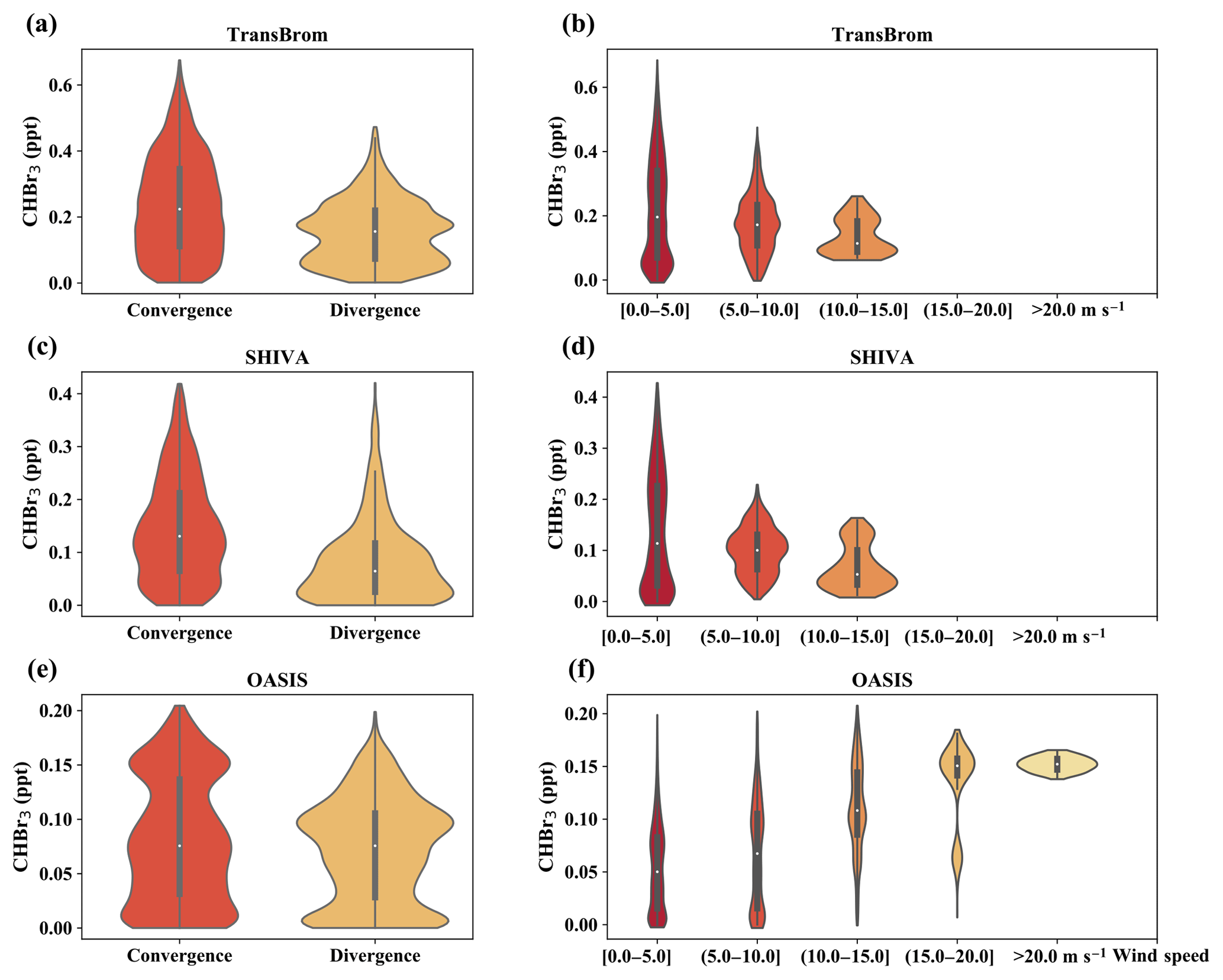
Figure 5 Violin plots of regional distributions of simulated background CHBr₃ mixing ratio by convergence and divergence (a, c, e) and by wind speed (b, d, f) at 1 km altitude averaged over TransBrom (a, b), SHIVA (c, d), and OASIS (e, f). The violin is a corresponding density plot with a boxplot inside. The white dots represent the medians. The thick black bars in the center represent the interquartile ranges. The thin black lines represent the rest of the distributions, except for the outliers.

In order to validate the hypothesis, we show a violin plot of regional background CHBr₃ mixing ratios related to convergence–divergence and to the wind speeds averaged over each simulation period in Fig. 5. For the TransBrom case, the averaged ranges of mixing ratios in regions of convergence and divergence (Fig. 5a) go up to 0.7 and 0.5 ppt, respectively, with interquartile ranges of 0.1–0.35 and 0.05–0.21 ppt. Probability of mixing ratios larger than 0.2 ppt is much higher for regions of convergence compared to regions of divergence. Meanwhile, in the regions grouped by wind speed (Fig. 5b), higher CHBr₃ mixing ratios are more likely to occur in regions with lower wind speeds (i.e., in the regions of 0.0–5.0 m s⁻¹, mixing ratios go up to 0.65 ppt, while in the regions of 10–15 m s⁻¹, mixing ratios only go up to 0.25 ppt). Similar distributions also occur for the SHIVA case. During the OASIS case, the CHBr₃ mixing ratios are much smaller than for the other two cases due to stronger winds. The highest mixing ratios (∼0.15 to ∼0.2 ppt) are found in the regions of convergence (Fig. 5e). However, higher mixing ratios are also generally found in the regions of higher wind speeds (Fig. 5f), as the regions of convergence are located in the regions of high wind speed during the OASIS case. The distributions suggest that in general higher CHBr₃ mixing ratios tend to occur in the regions of convergence or lower wind speed, with the exception of the OASIS case where extremely high winds occurred and coincided with regions of convergence.

The relationship mentioned above also holds on a global scale. The global distributions of atmospheric CHBr₃ based on background emissions and wind fields averaged over the time periods of the SHIVA and OASIS campaigns are presented in Figs. 6 and 7. We omit the time period of the TransBrom case since the background CHBr₃ distribution diagnosed for this period is very similar to the background found for the SHIVA period. The global CHBr₃ background mixing ratios (Figs. 6a and 7a) display a very heterogeneous distribution in spite of the uniform background emissions used for the simulations. High CHBr₃ mixing ratios are again generally located in the regions of convergence, which also generally correspond to low wind speeds on a global scale. For the SHIVA period (November 2011), particularly high CHBr₃ background values of 0.3 to 0.4 ppt are found along the Equator over the Maritime Continent, West Pacific, Indian Ocean, and at the west coast of Africa, all of which are characterized by particularly low winds. In the northern and southeast Pacific, the wind speed is generally higher, and the corresponding CHBr₃ values of less than 0.15 ppt are much lower than in the tropical region. For the OASIS period (July–August 2014), the global CHBr₃ distribution is mostly reversed compared to the SHIVA period and high winds over the Indian Ocean and Maritime Continent lead to low CHBr₃ abundance in this region. The North Pacific on the other hand, with low wind speeds, is now a region of intense accumulation leading to 0.3–0.4 ppt of CHBr₃. The tropical West Pacific is the only region that experiences relatively low winds during both seasons, and constantly shows high CHBr₃ for the SHIVA and OASIS time periods.

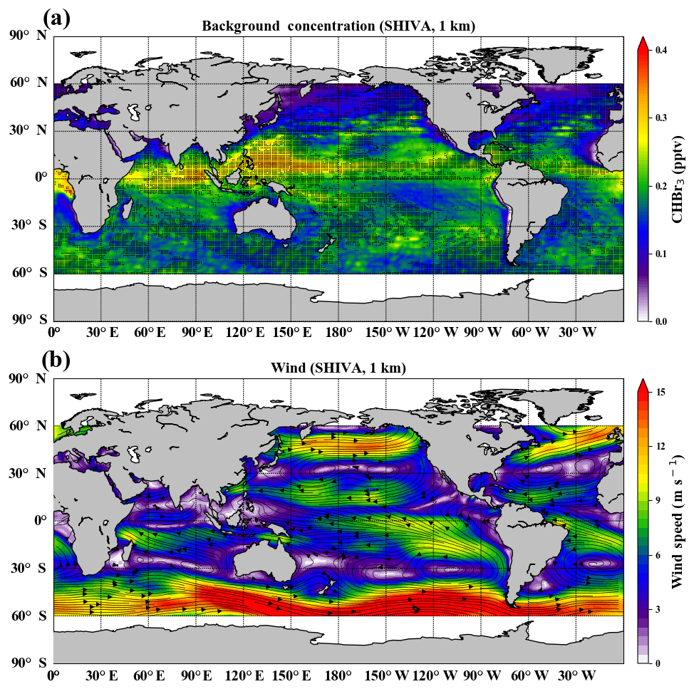
Figure 6 Global distributions of CHBr₃ mixing ratios based on oceanic background emissions (a) and ERA-Interim reanalysis wind fields (b) averaged during the time period of the SHIVA cruise at 1 km. The wind speeds are denoted by color shades and the directions are denoted by the stream lines. The regions of convergence are shaded in (a).

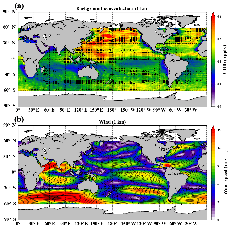
Figure 7 Same as Fig. 6, but for the OASIS case.

The variations in the background CHBr₃ distribution can be generally explained by the seasonal variations in the global wind field. The North Pacific and northern Indian Ocean are dominated by the East Asia Monsoon and the monsoon of South Asia, respectively. The East Asia Monsoon is characterized by strong northwesterly flow in boreal winter and weak southeasterly flow in boreal summer due to the reverse of the thermal gradient between land and ocean (Webster, 1987; Ding and Chan, 2005). Therefore, the accumulations of CHBr₃ in the North Pacific occur during the boreal summer months, rather than during boreal autumn and early winter (TransBrom time period). The monsoon of South Asia, on the other hand, is characterized by weak northeasterly winds in boreal winter and strong southwesterly winds in boreal summer (Webster, 1987; Webster et al., 1998). Thus background CHBr₃ accumulation over the northern Indian Ocean occurs mostly during boreal winter, while during boreal summer (OASIS time period) a low CHBr₃ background can be expected. Because of the light winds of the Inter-tropical Convergence Zone (ITCZ), a belt of relatively high CHBr₃ abundance exists along the Equator in the Northern Hemisphere, especially in the tropical Pacific and Atlantic. Strong convection in the ITCZ enhances vertical transport of CHBr₃ out of the boundary layer, but overall the CHBr₃ distribution is dominated by the horizontal wind fields and accompanying transport patterns. Due to the more complex land–sea thermal difference, the seasonal variations in ITCZ in the West Pacific is more significant than in the East Pacific (Waliser and Jiang, 2014). The relatively high accumulations of CHBr₃ in the tropical East Pacific are confined to a narrow region near the Equator for both seasons. As for the tropical West Pacific, during boreal winter the ITCZ covers almost all of Southeast Asia and the high CHBr₃ abundances during SHIVA appear along the east coast of Malaysia. During boreal summer, the ITCZ shifts northward and the high CHBr₃ abundances retreat northwestward.

In the above simulations, we assume a constant background emission in order to isolate the impact of transport and loss processes on the atmospheric CHBr₃ distribution. Variations in the wind fields will likely impact the oceanic air–sea flux and emissions. Such variations can change the background CHBr₃ distribution and may allow for increased mixing ratios in regions of strong winds. In addition to the wind speed, variations in the atmospheric and, more importantly, the oceanic CHBr₃ concentrations can impact the emission strength, which can further change the complex atmospheric CHBr₃ distribution.

4 Atmospheric CHBr₃ based on hot spot emissions

Given the high variability of the atmospheric CHBr₃ background mixing ratios, resulting from atmospheric transport processes (Sect. 3), it is of interest to analyze if and how much oceanic hot spot emissions might impact this background distribution. In this section, the results of simulations based on observed localized hot spot emissions will be compared to the background mixing ratios.

4.1 Observed hot spot emissions

Oceanic CHBr₃ emissions, atmospheric CHBr₃ mixing ratios, and the observed local surface wind speeds are given in Fig. 8 for all three campaigns. The oceanic emissions of CHBr₃ vary substantially from campaign to campaign with mean values of 261 pmol h⁻¹ m⁻² (TransBrom), 1228 pmol h⁻¹ m⁻² (SHIVA), and 912 pmol h⁻¹ m⁻² (OASIS) with standard deviations of 600 pmol h⁻¹ m⁻² (TransBrom), 1460 pmol h⁻¹ m⁻² (SHIVA), and 1159 pmol h⁻¹ m⁻² (OASIS), respectively (Tegtmeier et al., 2012; Ziska et al., 2013; Fuhlbrügge et al., 2016; Fiehn et al., 2017).

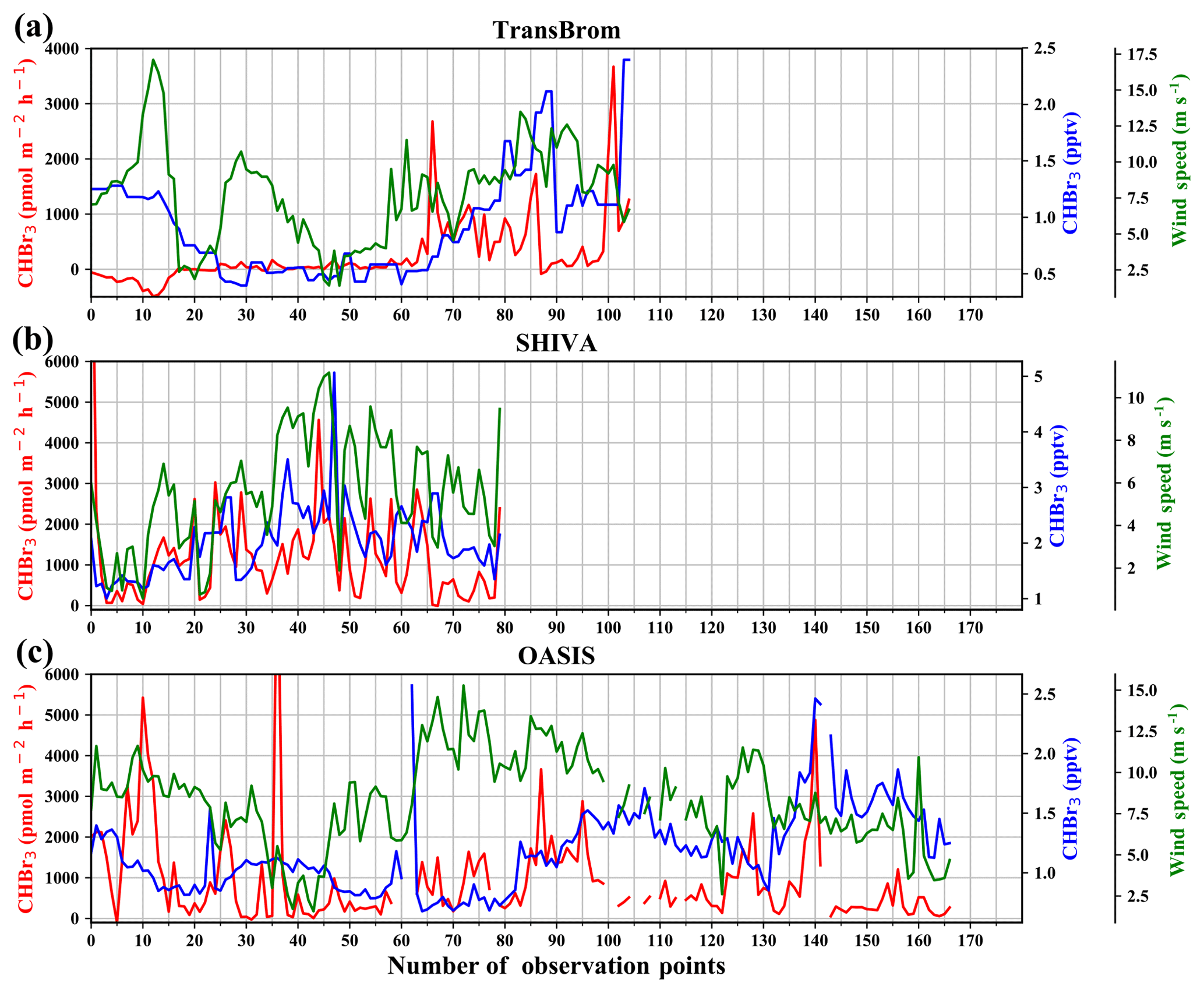
Figure 8 Surface wind speeds (green), CHBr₃ air–sea flux (red), and atmospheric mixing ratios of CHBr₃ near the surface (blue) observed during the TransBrom, SHIVA, and OASIS campaigns.

All three campaigns show periods with localized elevated and hot spot emissions. For TransBrom, the first two-thirds of the campaign show negative (into the ocean) or very low CHBr₃ fluxes, while the last third was close to western Pacific islands and is characterized by overall elevated emissions with sporadic hot spots of up to 4000 pmol h⁻¹ m⁻². The SHIVA cruise track was mostly along the coastline, where elevated emissions and hot spots occurred regularly. The OASIS cruise track alternated between open ocean, upwelling, and coastal areas, resulting in a large fluctuation between low background and localized elevated emissions. The largest hot spot emissions were observed during this campaign, reaching values of over 6000 pmol h⁻¹ m⁻².

According to the flux parameterization applied here, the variability of air–sea flux is determined mostly by the surface wind speed and the ocean–atmosphere concentration gradient. The highest emissions are expected to occur during periods of high wind speeds and large concentration gradients. During the beginning of the TransBrom campaign (Fig. 8a), the wind speed peaks at over 15 m s⁻¹ while the corresponding CHBr₃ air–sea flux is low. Higher wind speeds co-occur with high air–sea fluxes at the end of the campaign. For SHIVA (Fig. 8b) and OASIS (Fig. 8c), the relation between wind speed and CHBr₃ emissions is more easily discernable.

All three campaigns demonstrate that high fluxes do not always lead to local high CHBr₃ mixing ratios in the surface atmosphere. For example, several hot spots with oceanic emissions over 4000 pmol m⁻² h⁻¹ are found during OASIS; however, corresponding atmospheric mixing ratios are relatively low (∼2 ppt). Vice versa, the highest atmospheric mixing ratios found during OASIS only coincide with high fluxes during the last part of the campaign. These discrepancies underline how the complex interplay of source, transport, and loss processes impact on the local atmospheric mixing ratios of short-lived compounds. A relatively clear connection between elevated oceanic emissions and surface mixing ratios only occurs during the SHIVA campaign and during the last part of the TransBrom campaign (Fig. 8a and b).

The question arises of how much of the atmospheric variability of short-lived compounds such as CHBr₃ is impacted by the emission strengths and is addressed in the subsequent section based on the model results.

4.2 Comparison of CHBr₃ from background and hot spot emissions

In this section, we compare the concentrations of CHBr₃ due to background and localized elevated emissions as simulated by FLEXPART. Atmospheric background and hot spot CHBr₃ at different altitudes is simulated by FLEXPART, which is driven by the meteorological data from ECMWF. The signatures of dynamical processes such as wind regimes, weather phenomena (e.g., typhoons), and convection are captured by the model simulation and can be detected in the CHBr₃ distribution (Fig. 9). For example, during the TransBrom campaign, the cruise encountered several tropical storms in the western Pacific, one of which (Lupit, around 14 October 2009) developed into a super typhoon within several days (Krüger and Quack, 2013). As shown in Fig. 9, CHBr₃ accumulation representing the structure of typhoon Lupit is clearly visible in the background distribution of CHBr₃ at 500 m altitude (Fig. 9d) in the northern part of the western Pacific. This structure is still clear at 5 km altitude (Fig. 9a), although with a weaker magnitude. Localized elevated sources of CHBr₃ (Fig. 9b, c, e, and f) do not add much due to the small spatial extent of the 0.5 or 1^∘ emission cells, and thus the limited amount of overall released CHBr₃ is not discernible in the large-scale structures. Higher abundances of atmospheric CHBr₃ can be seen in the southern part of the western Pacific near Indonesia resulting from one of the hot spot emissions observed during TransBrom (Fig. 1b). However, the background CHBr₃ in this area is also high in this low-wind area, and thus the atmospheric signal of the up to 20 times stronger hot spot emissions (Fig. 8a) is not detectable for either the 0.5^∘ or the 1^∘ wide emission cells when compared to the background. Note that the modeled atmospheric mixing ratios from both sources, hot spot and background emissions, are smaller than the mixing ratios observed along the cruise track (Fig. 8), suggesting stronger nearby emissions not covered in our scenarios and observations. The signature of the hot spot emissions cannot be seen at 5 km altitude.

Figure 9 Atmospheric CHBr₃ mixing ratios at different altitudes (500 m and 5 km) simulated for the time period of the TransBrom campaign. Simulations are based on background emissions (a, d) and elevated emissions observed during the campaign for 0.5^∘ (b, e) and 1^∘ (c, f) wide emission grid cells.

Figure 10 shows the atmospheric CHBr₃ mixing ratios during the SHIVA campaign. The atmospheric signal of the localized elevated emissions during SHIVA is much stronger than during TransBrom due to stronger emissions and smaller background mixing ratios. First, for the 0.5^∘ wide emission grids, two highly localized atmospheric CHBr₃ peaks appear close to the coastline near the Equator around 105^∘ E with a maximum value around 0.4 ppt. These signals occur in a spot where the background is very low (0.2 ppt). However, at the same time they are smaller than the maximum background values of up to 0.5 ppt in nearby regions (Fig. 10d). If the width of the emission grids is extended to 1^∘, the localized CHBr₃ peaks mentioned above grow into two distinct blobs near the Equator of up to 0.8 ppt, which are apparently larger than the regional background concentrations (Fig. 10f). Elevated emissions during the second half of the campaign with several hot spot events, on the other hand, do not show such clear atmospheric signals right above.

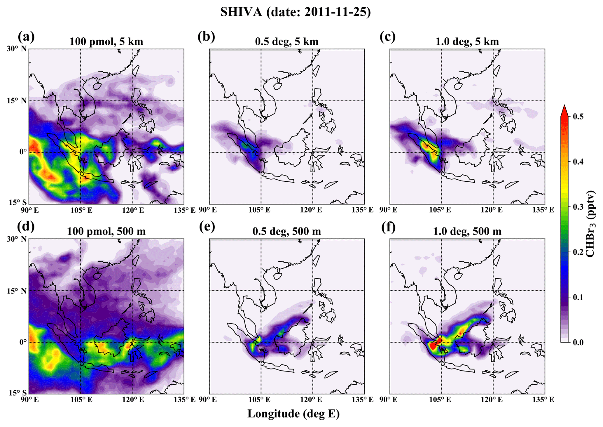
Figure 10 Same as Fig. 9, but for the SHIVA campaign.

For the regions of localized elevated emissions, the convection is less effective and maximum mixing ratios at 5 km are about 50 % smaller compared to the values in the boundary layer. Thus only the signal of the 1^∘ wide emission cells can be detected at 5 km, while assuming that the emissions covering a smaller region of 0.5^∘ width will render their impact in the free troposphere negligible. Krysztofiak et al. (2018) calculated the fractions of convective-contributed trace gases from the boundary layer to the upper troposphere using airborne measurements during the SHIVA campaign and reported an even smaller fraction of boundary layer CHBr₃ in the upper troposphere (about 15 % due to convection).

Due to the dominant southwest monsoon over the northern Indian Ocean in boreal summer, the resulting atmospheric abundances of the OASIS case (Fig. 11) for both scenarios, background and localized emissions, are much lower than for the other two campaigns. This is particularly surprising for the OASIS hot spot emissions, which are in many cases larger than hot spot emissions during TransBrom or SHIVA. In the open ocean, the atmospheric enhanced CHBr₃ mixing ratios resulting from the 0.5^∘ (1^∘) wide localized emission runs reach only 0.1 (0.2) ppt in a narrow belt near 60^∘ E and are mostly smaller than the background (around 0.15 ppt). An exception occurs near the coast of Madagascar, where both background and hot spot emissions accumulate in the atmosphere. Maximum background values reach up to 0.25 ppt and the hot spot signals peak with values of 0.3 ppt (0.5^∘ wide emission cells) to 0.6 ppt (1^∘ wide emissions cells). These clear atmospheric signals of hot spot emissions are driven by the enhanced coastal emissions near Madagascar. At 5 km altitude, atmospheric background values are very low, and the hot spot contributions are close to zero.

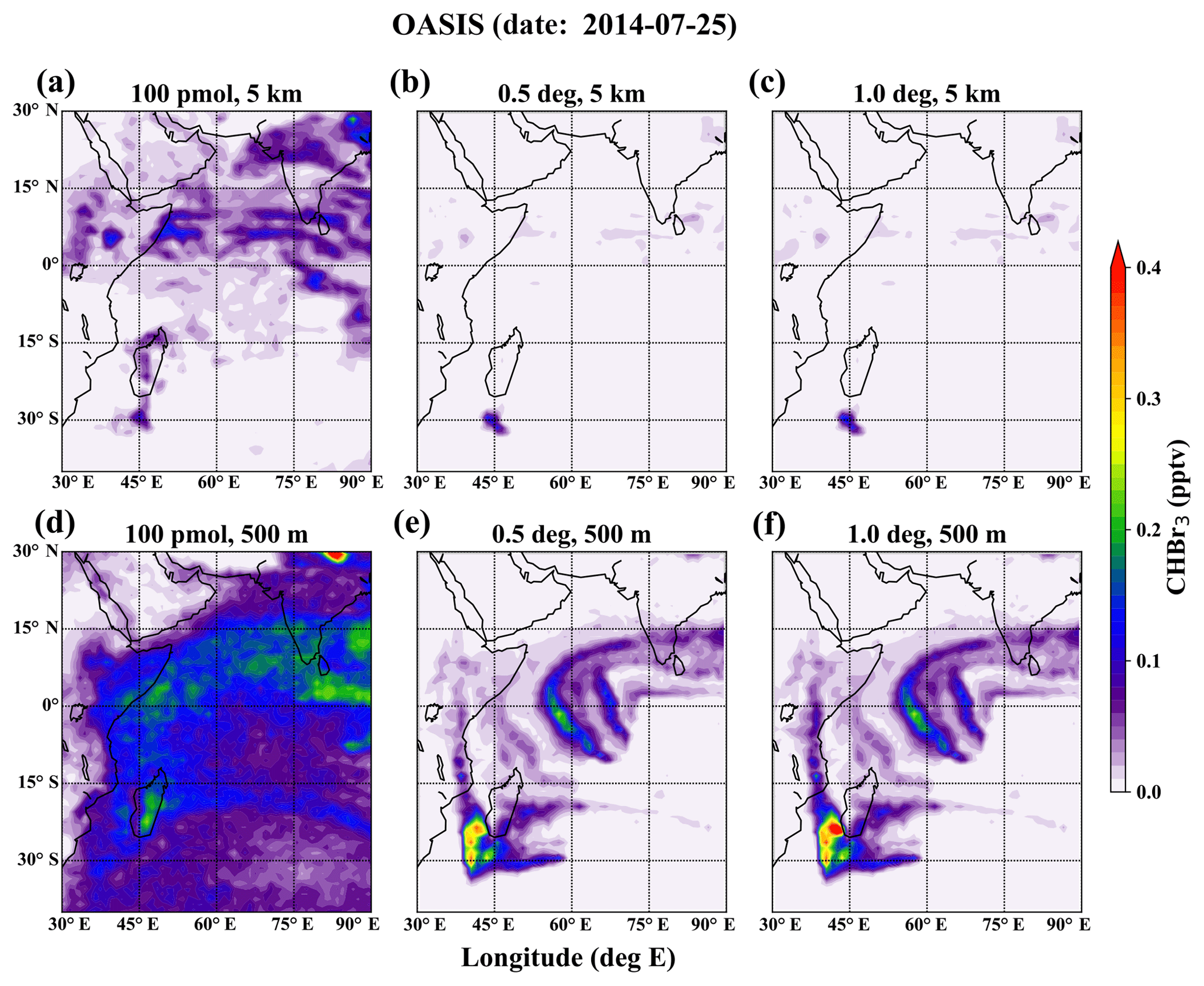
Figure 11 Same as Fig. 9, but for the OASIS campaign.

In summary, although the observed emissions during the three cruises were significantly higher than the background of 100 pmol m⁻² h⁻¹, our results show that such strong oceanic sources are not necessarily detectable in the atmosphere, where transport processes can mask the impact of oceanic emissions.

5 Summary and discussion

In this study, we simulated atmospheric CHBr₃ abundances that result from uniform marine background emissions compared to hot spot emissions using the Lagrangian dispersion model FLEXPART.

The simulations demonstrate that uniform background emissions from the ocean result in a highly variable atmospheric CHBr₃ distribution with high mixing ratios taking place in regions of convergence or low wind speed. This relation holds on regional and global scales, underlining the role of atmospheric transport processes as drivers of the distribution of short-lived trace gases with lifetimes in the range of days to weeks. The relation between atmospheric background and wind patterns described here will allow us to better predict the seasonal and regional characteristics of the tropospheric CHBr₃ distribution. Such knowledge will provide valuable information for analyzing and interpreting atmospheric data from ship and aircraft campaigns. For example, our results illustrate that elevated or low atmospheric CHBr₃ abundances cannot necessarily be used to draw conclusions about the oceanic source strength below.

Comparisons between atmospheric CHBr₃ resulting from background and peak emissions suggest that the impact of localized elevated emissions on the atmospheric CHBr₃ distribution depends on their relative strength, on their location, and on the time of emission. The “visibility” of elevated emissions in the atmospheric CHBr₃ distribution varies significantly between three cruises in the West Pacific and Indian oceans. In the open ocean, signals of elevated emissions can hardly be distinguished from the background CHBr₃ distribution even for elevated sources extending over 1^∘ wide source regions along the cruise tracks. Near the coast, however, signals of elevated emissions are often stronger to be distinguished from the background, in particular, hot spot emissions up to 100 times larger than the background. However, individual cases show that it is not necessarily the largest hot spot that gives a clear signal, but that the tug-of-war between fast advective transport and local accumulation at the time of emission is also important.

Our approach requires that we isolate uniform background CHBr₃ emission from coastal and shelf emissions, which can be significant (Fuhlbrügge et al., 2016; Fiehn et al., 2017) and would lead to higher atmospheric abundances. As a consequence, we expect the background CHBr₃ mixing ratios inferred from our simulations to be smaller compared to observations and other modeling studies. In the western Pacific (TransBrom), our simulated background mixing ratios at 5 km range from 0.0 to 0.4 ppt (Figs. 9–11). Measurements from aircraft campaigns in this region, CAST (Harris et al., 2016) and CONTRAST (Pan et al., 2016), show higher CHBr₃ mixing ratios of 0.03–0.79 and 0.20–1.127 ppt between 4 and 6 km. Other model studies (e.g., Hossaini et al., 2016; Butler et al., 2018) based on CHBr₃ emission scenarios that include coastal and open ocean sources (e.g., Liang et al., 2010; Ordóñez et al., 2012; Ziska et al., 2013) also suggest the average CHBr₃ mixing ratio over 0.5 ppt in this region.

The constant background emissions of 100 pmol m⁻² h⁻¹ used in our study are based on a simplified scenario and do not include coastal emissions. Nevertheless, our results demonstrate that atmospheric CHBr₃ signals, produced by localized elevated and even hot spot emissions, orders of magnitudes larger than the average open ocean emissions, can be obliterated by the highly variable atmospheric background. That is to say that transport variations in the atmosphere itself are sufficient to allow high concentrations in certain regions and that high concentrations of VSLH in the atmosphere do not always guarantee a strong local or regional source. For observational and modeling studies of VSLHs and other short-lived compounds, the impact of atmospheric transport patterns that are identified here can be used for the interpretation of trace gas distributions and variability.