Simulating CH₄ and CO₂ over South and East Asia using the zoomed chemistry transport model LMDz-INCA

The increasing availability of atmospheric measurements of greenhouse gases (GHGs) from surface stations can improve the retrieval of their fluxes at higher spatial and temporal resolutions by inversions, provided that transport models are able to properly represent the variability of concentrations observed at different stations. South and East Asia (SEA; the study area in this paper including the regions of South Asia and East Asia) is a region with large and very uncertain emissions of carbon dioxide (CO₂) and methane (CH₄), the most potent anthropogenic GHGs. Monitoring networks have expanded greatly during the past decade in this region, which should contribute to reducing uncertainties in estimates of regional GHG budgets. In this study, we simulate concentrations of CH₄ and CO₂ using zoomed versions (abbreviated as “ZAs”) of the global chemistry transport model LMDz-INCA, which have fine horizontal resolutions of ∼0.66^∘ in longitude and ∼0.51^∘ in latitude over SEA and coarser resolutions elsewhere. The concentrations of CH₄ and CO₂ simulated from ZAs are compared to those from the same model but with standard model grids of 2.50^∘ in longitude and 1.27^∘ in latitude (abbreviated as “STs”), both prescribed with the same natural and anthropogenic fluxes. Model performance is evaluated for each model version at multi-annual, seasonal, synoptic and diurnal scales, against a unique observation dataset including 39 global and regional stations over SEA and around the world. Results show that ZAs improve the overall representation of CH₄ annual gradients between stations in SEA, with reduction of RMSE by 16–20 % compared to STs. The model improvement mainly results from reduction in representation error at finer horizontal resolutions and thus better characterization of the CH₄ concentration gradients related to scattered distributed emission sources. However, the performance of ZAs at a specific station as compared to STs is more sensitive to errors in meteorological forcings and surface fluxes, especially when short-term variabilities or stations close to source regions are examined. This highlights the importance of accurate a priori CH₄ surface fluxes in high-resolution transport modeling and inverse studies, particularly regarding locations and magnitudes of emission hotspots. Model performance for CO₂ suggests that the CO₂ surface fluxes have not been prescribed with sufficient accuracy and resolution, especially the spatiotemporally varying carbon exchange between land surface and atmosphere. In addition, the representation of the CH₄ and CO₂ short-term variabilities is also limited by model's ability to simulate boundary layer mixing and mesoscale transport in complex terrains, emphasizing the need to improve sub-grid physical parameterizations in addition to refinement of model resolutions.

1 Introduction

Despite attrition in the global network of greenhouse gas (GHG) monitoring stations (Houweling et al., 2012), new surface stations have been installed since the late 2000s in the northern industrialized continents such as Europe (e.g., Aalto et al., 2007; Lopez et al., 2015; Popa et al., 2010), North America (e.g., Miles et al., 2012) and Northeast Asia (e.g., Fang et al., 2014; Sasakawa et al., 2010; Wada et al., 2011; Winderlich et al., 2010). In particular, the number of continuous monitoring stations over land has increased (e.g., Aalto et al., 2007; Lopez et al., 2015; Winderlich et al., 2010) given that more stable and precise instruments are available (e.g., Yver Kwok et al., 2015). These observations can be assimilated in inversion frameworks that combine them with a chemistry transport model and prior knowledge of fluxes to optimize GHG sources and sinks (e.g., Berchet et al., 2015; Bergamaschi et al., 2010, 2015; Bousquet et al., 2000, 2006; Bruhwiler et al., 2014; Gurney et al., 2002; Peters et al., 2010; Rödenbeck et al., 2003). Given the increasing observation availability, GHG budgets are expected to be retrieved at finer spatial and temporal resolutions by atmospheric inversions if the atmospheric GHG variability can be properly modeled at theses scales. A first step of any source optimization is to evaluate the ability of chemistry transport models to represent the variabilities of GHG concentrations, as transport errors are recognized as one of the main uncertainties in atmospheric inversions (Locatelli et al., 2013).

Many previous studies have investigated regional and local variations of atmospheric GHG concentrations using atmospheric chemistry transport models, with spatial resolutions ranging 100–300 km for global models (e.g., Chen and Prinn, 2005; Feng et al., 2011; Law et al., 1996; Patra et al., 2009a, b) and 10–100 km for regional models (e.g., Aalto et al., 2006; Chevillard et al., 2002; Geels et al., 2004; Wang et al., 2007). Model intercomparison experiments showed that the atmospheric transport models with higher horizontal resolutions are more capable of capturing the observed short-term variability at continental sites (Geels et al., 2007; Law et al., 2008; Maksyutov et al., 2008; Patra et al., 2008; Saeki et al., 2013), due to reduction of representation errors (point-measured vs. grid-box-averaged modeled concentrations), improved model transport, and more detailed description of surface fluxes and topography (Patra et al., 2008). However, a higher horizontal model resolution also demands high-quality meteorological forcings and prescribed surface fluxes as boundary conditions (Locatelli et al., 2015a).

Two main approaches have been deployed, in an Eulerian modeling context, to address the need for high-resolution transport modeling of long-lived GHGs. The first approach is to define a high-resolution grid mesh in a limited spatial domain of interest and to nest it within a global model with varying degrees of sophistication to get boundary conditions for the GHGs advected inside and outside the regional domain (Bergamaschi et al., 2005, 2010; Krol et al., 2005; Peters et al., 2004). The second approach is to stretch the grid of a global model over a specific region (the so-called “zooming”) while maintaining all parameterizations consistent (Hourdin et al., 2006). For the former approach, several nested high-resolution zooms can be embedded into the same model (Krol et al., 2005) to focus on different regions. The zooming approach has the advantage of avoiding the nesting problems (e.g., tracer discontinuity, transport parameterization inconsistency) at the boundaries between a global and a regional model. In this study, we use the zooming capability of the LMDz model (Hourdin et al., 2006).

South and East Asia (hereafter “SEA”) has been the largest anthropogenic GHG-emitting region since the mid-2000s due to its rapid socioeconomic development (Marland et al., 2015; Olivier et al., 2015; Le Quéré et al., 2015; Tian et al., 2016). Compared to Europe and North America where sources and sinks of GHGs are partly constrained by atmospheric observational networks, the quantification of regional GHG fluxes over SEA from atmospheric inversions remains uncertain due to the low density of surface observations (e.g., Patra et al., 2013; Swathi et al., 2013; Thompson et al., 2014, 2016). During the past decade, a number of new surface stations have been deployed (e.g., Fang et al., 2016, 2014; Ganesan et al., 2013; Lin et al., 2015; Tiwari and Kumar, 2012), which have the potential to provide new and useful constraints on estimates of GHG fluxes in this region. However, modeling GHG concentrations at these stations is challenging since they are often located in complex terrains (e.g., coasts or mountains) or close to large local sources of multiple origins. To fully take advantage of the new surface observations in SEA, forward modeling studies based on high-resolution transport models are needed to evaluate the ability of the inversion framework to assimilate such new observations.

In this study, we apply the chemistry transport model LMDz-INCA (Folberth et al., 2006; Hauglustaine et al., 2004; Hourdin et al., 2006; Szopa et al., 2013) zoomed to a horizontal resolution of ∼50 km over SEA to simulate the variations of CH₄ and CO₂ during the period 2006–2013. The model performance is evaluated against observations from 39 global and regional stations inside and outside the zoomed region. The variability of the observed or simulated concentrations at each station is decomposed for evaluation at different temporal scales, namely the annual mean gradients between stations, the seasonal cycle, the synoptic variability and the diurnal cycle. For comparison, a non-zoomed standard version (ST) of the same transport model is also run with the same set of surface fluxes to estimate the improvement gained from the zoomed configuration. The detailed description of the observations and the chemistry transport model is presented in Sect. 2, together with the prescribed CH₄ and CO₂ surface fluxes that force the simulations, as well as the metrics used to quantify the model performance. The evaluation of the simulations performed is presented and discussed in Sect. 3, showing capabilities of the transport model to represent the annual gradients between stations, as well as the seasonal, synoptic, and diurnal variations. Conclusions and implications drawn from this study are given in Sect. 4.

2 Data and methods

2.1 Model description

2.1.1 LMDz-INCA

The LMDz-INCA model couples a general circulation model developed at the Laboratoire de Météorologie Dynamique (LMD; Hourdin et al., 2006) and a global chemistry and aerosol model INteractions between Chemistry and Aerosols (INCA; Folberth et al., 2006; Hauglustaine et al., 2004). A more recent description of LMDz-INCA is presented in Szopa et al. (2013). To simulate CH₄ and CO₂ concentrations, we run a standard version of the model with a horizontal resolution of 2.5^∘ in longitude (i.e., 144 model grids) and 1.27^∘ in latitude (i.e., 142 model grids) (hereafter this version is abbreviated as “STs”) and a zoomed version with the same number of grid boxes, but a resolution of ∼0.66^∘ in longitude and ∼0.51^∘ in latitude in a region of 50–130^∘ E and 0–55^∘ N centered over India and China (hereafter this version is abbreviated as “ZAs”) (Fig. 1; see also Wang et al., 2014, 2016). It means that, in terms of the surface area, a grid cell from STs roughly contains 9 grid-cells from ZAs within the zoomed region. Both model versions are run with 19 and 39 sigma-pressure layers, thus rendering four combinations of horizontal and vertical resolutions (i.e., ST19, ZA19, ST39, ZA39). Vertical diffusion and deep convection are parameterized following the schemes of Louis (1979) and Tiedtke (1989), respectively. The simulated horizontal wind vectors (u and v) are nudged towards the 6-hourly European Center for Medium Range Weather Forecast (ECMWF) reanalysis dataset (ERA-I) in order to simulate the observed large-scale advection (Hourdin and Issartel, 2000).

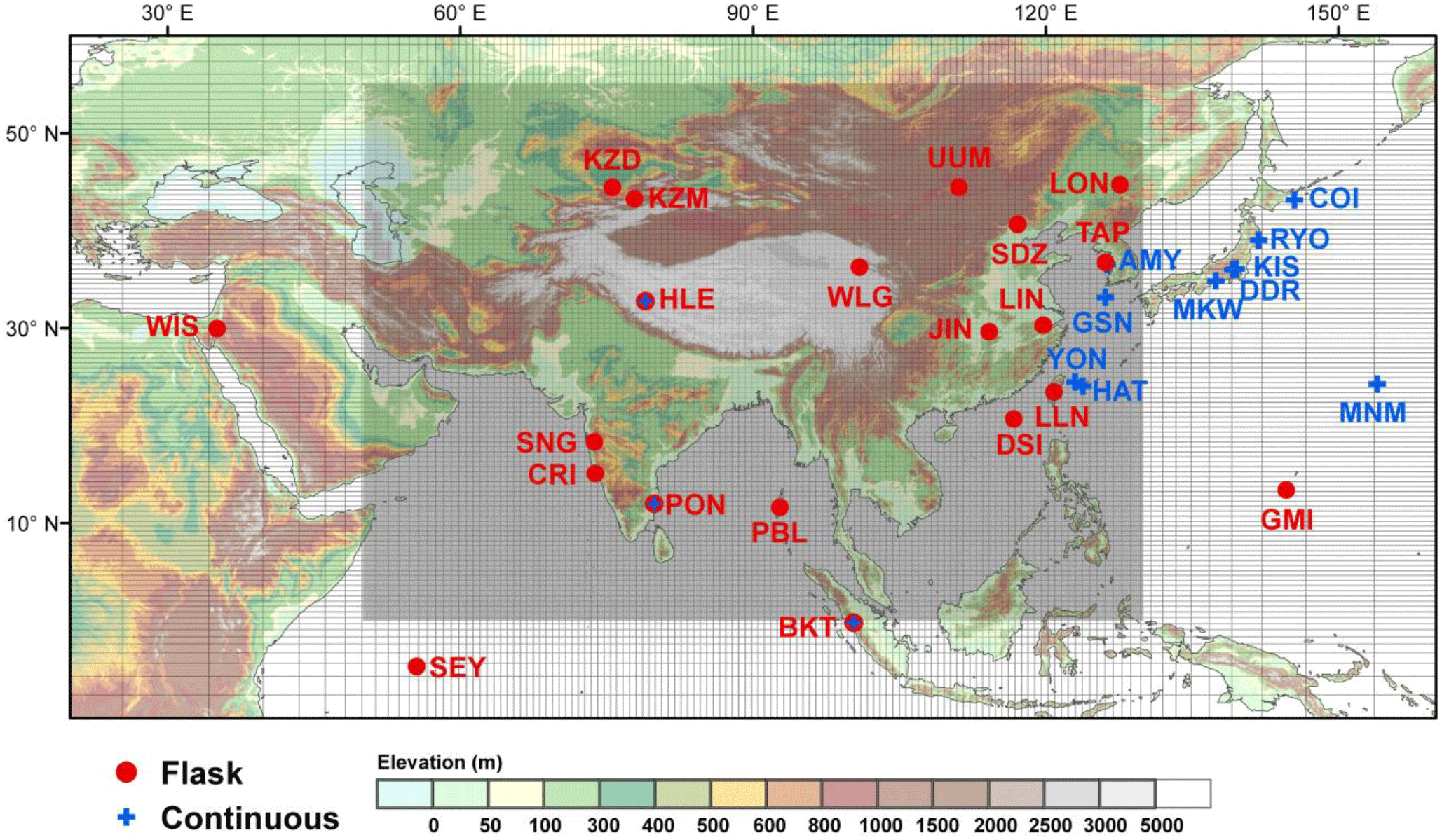
Figure 1 Map of locations of stations within and around the zoomed region. The zoomed grid of the LMDz-INCA model is plotted with the NASA Shuttle Radar Topographic Mission (SRTM) 1 km digital elevation data (DEM) as background (http://srtm.csi.cgiar.org, last access: 6 March 2015). The grey shaded area indicates the region with a horizontal resolution of ∼0.66^∘ $\times \sim \mathrm{0.51}$^∘. The red close circle (blue cross) represents the atmospheric station where flask (continuous) measurements are available and used in this study.

The atmospheric concentrations of hydroxyl radicals (OH), the main sink of atmospheric CH₄, are produced from a simulation at a horizontal resolution of 3.75^∘ in longitude (i.e., 96 model grids) and 1.9^∘ in latitude (i.e., 95 model grids) with the full INCA tropospheric photochemistry scheme (Folberth et al., 2006; Hauglustaine et al., 2004, 2014). The OH fields are climatological monthly data and are regridded to the standard and zoomed model grids, respectively. It should be noted that the spatiotemporal distributions of the OH concentrations have large uncertainties and vary greatly among different chemical transport models; therefore, the choice of the OH fields may affect the evaluation for CH₄ (especially in terms of the annual gradients between stations and the seasonal cycles). In this study, as we focus more on the improvement of performance gained from refinement of the model resolution rather than model–observation misfits and model bias in CH₄ growth rates, the influences of OH variations on model improvement are assumed to be very small given that the OH fields for both ZAs and STs are regridded from a lower model resolution and thus don't show much difference between the two model versions.

The CH₄ and CO₂ concentrations are simulated over the period 2000–2013 with both STs and ZAs. The first 6 years (2000–2005) of the simulations are considered as model spin-up; thus, we only compare the simulated CH₄ and CO₂ concentrations with observations during 2006–2013. The initial CH₄ concentration field is defined based on the optimized initial state from a CH₄ inversion that assimilates observations from 50+ global background stations over the period 2006–2012 (Locatelli, 2014; Locatelli et al., 2015b). The optimized initial CH₄ concentration field for the year 2006 is rescaled to the levels of the year 2000 and used as the initial state in our simulations. The time step of model outputs is hourly.

2.1.2 Prescribed CH₄ and CO₂ surface fluxes

The prescribed CH₄ and CO₂ surface fluxes used as model inputs are presented in Table 1. We simulate the CH₄ concentration fields using a combination of the following datasets: (1) the interannually varying anthropogenic emissions obtained from the Emission Database for Global Atmospheric Research (EDGAR) v4.2 FT2010 product (http://edgar.jrc.ec.europa.eu, last access: 21 October 2016), including emissions from rice cultivation with the seasonal variations based on Matthews et al. (1991) imposed to the original yearly data; (2) climatological wetland emissions based on the scheme developed by Kaplan et al. (2006); (3) interannually and seasonally varying biomass burning emissions from Global Fire Emissions Database (GFED) v4.1 product (Randerson et al., 2012; Van Der Werf et al., 2017; http://www.globalfiredata.org/, last access: 3 May 2017); (4) climatological termite emissions (Sanderson, 1996); (5) climatological ocean emissions (Lambert and Schmidt, 1993); and (6) climatological soil uptake (Ridgwell et al., 1999). Note that for anthropogenic emissions from sectors other than rice cultivation, the seasonal variations are much smaller, and a monthly sector-specific dataset is currently not available for the whole study period. Therefore we do not consider seasonal variations in CH₄ emissions from those sectors. Based on these emission fields, the global CH₄ emissions in 2010 are 543 Tg CH₄ yr⁻¹ and 191 Tg CH₄ yr⁻¹ over the zoomed region. For the years over which CH₄ anthropogenic emissions were not available from the data sources when the simulations were performed (namely, the years 2011–2013), we use emissions for the year 2010.

Table 1 The prescribed CH₄ and CO₂ surface fluxes used as model input. For each trace gas, magnitudes of different types of fluxes are given for the year 2010. Total_global and Total_zoom indicate the total flux summarized over the globe and the zoomed region, respectively.

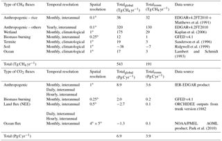
The prescribed CO₂ fluxes used to simulate the concentration fields are based on the following datasets: (1) three variants (hourly, daily and monthly means) of interannually varying fossil fuel emissions produced by the Institut für Energiewirtschaft und Rationelle Energieanwendung (IER), Universität Stuttgart, on the basis of EDGARv4.2 product (hereafter IER-EDGAR, http://carbones.ier.uni-stuttgart.de/wms/index.html, last access: 14 December 2014) (Pregger et al., 2007); (2) interannually and seasonally varying biomass burning emission from GFEDv4.1 (Randerson et al., 2012; Van Der Werf et al., 2017; http://www.globalfiredata.org/, last access: 3 March 2017); (3) interannually and hourly varying terrestrial biospheric fluxes produced from outputs of the Organizing Carbon and Hydrology in Dynamic EcosystEms (ORCHIDEE) model; and (4) interannually and seasonally varying air–sea CO₂ gas exchange maps developed by NOAA's Pacific Marine Environmental Laboratory (PMEL) and Atlantic Oceanographic and Meteorological Laboratory (AOML) groups (Park et al., 2010). Here ORCHIDEE runs with the trunk version r1882 (source code available at http://forge.ipsl.jussieu.fr/orchidee/wiki/SourceCode/ORCHIDEE, last access: 3 June 2018, with the revision number of r1882), using the same simulation protocol as the SG3 simulation in MsTMIP project (Huntzinger et al., 2013). The climate forcing data are obtained from CRUNCEP v5.3.2, while the yearly land use maps, soil map and other forcing data (e.g., monthly CO₂ concentrations) are as described in Wei et al. (2014). The sums of global net CO₂ surface fluxes in 2010 are 6.9 Pg C yr⁻¹ and 3.9 Pg C yr⁻¹ over the zoomed region. For the CO₂ fossil fuel emissions, the IER-EDGAR product is only available until 2009. To generate the emission maps for the years 2010–2013, we scale the emission spatial distribution in 2009 using the global totals for these years based on the EDGARv4.2FT2010 datasets. The detailed information for each surface flux is listed in Table 1.

2.2 Atmospheric CH₄ and CO₂ observations

The simulated CH₄ and CO₂ concentrations are evaluated against observations from 39 global and regional stations within and outside the zoomed region, operated by different programs and organizations (Fig. 1; Table 2). The stations where flask observations are published (25 stations in total) mainly belong to the cooperative program organized by the NOAA Earth System Research Laboratory (NOAA∕ESRL, available at ftp://aftp.cmdl.noaa.gov/data/trace_gases/, last access: 7 Octoeber 2017). We also use flask observations from stations operated by the China Meteorological Administration (CMA, China) (the JIN, LIN and LON stations, see also Fang et al., 2014), Commonwealth Scientific and Research Organization (CSIRO, Australia) (the CRI station, Bhattacharya et al., 2009, available at http://ds.data.jma.go.jp/gmd/wdcgg/, last access: 7 October 2017), Indian Institute of Tropical Meteorology (IITM, India) (the SNG station; see also Tiwari et al., 2014) and stations from the Indo-French cooperative research program (the HLE, PON and PBL stations, Lin et al., 2015; Swathi et al., 2013). All the CH₄ (CO₂) flask measurements are reported on or linked to the NOAA2004 (WMOX2007) calibration scale, which guarantees comparability between stations in terms of annual means.

Table 2 Stations used in this study. For the column “Zoom”, “Y” indicates a station within the zoomed region.

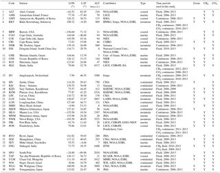
Abbreviations: Aichi – Aichi Air Environment Division, Japan; AIES – Arava Institute for Environmental Studies, Israel; BMKG – Agency for Meteorology, Climatology and Geophysics, Indonesia; CMA – China Meteorological Administration, China; CSIR4PI – Council of Scientific and Industrial Research Fourth Paradigm Institute, India; CSIRO – Commonwealth Scientific and Industrial Research Organisation, Australia; Empa – Swiss Federal Laboratories for Materials Science and Technology, Switzerland; ESSO/NIOT – Earth System Sciences Organisation/National Institute of Ocean Technology, India; IIA – Indian Institute of Astrophysics, India; IITM – Indian Institute of Tropical Meteorology, India; JMA – Japan Meteorological Agency, Japan; KCAER – Korea Centre for Atmospheric Environment Research, Republic of Korea; KMA – Korea Meteorological Administration, Republic of Korea; KSIEMC – Kazakh Scientific Institute of Environmental Monitoring and Climate, Kazakhstan; LAIBS – Lulin Atmospheric Background Station, Taiwan; LSCE – Laboratoire des Sciences du Climat et de l'Environnement, France; MHRI – Mongolian Hydrometeorological Research Institute, Mongolia; NIER – National Institute of Environmental Research, Republic of Korea; NIES – National Institute for Environmental Studies, Japan; NIWA – National Institute of Water and Atmospheric Research, New Zealand; NOAA/ESRL – National Oceanic and Atmospheric Administration/Earth System Research Laboratory; Saitama – Center for Environmental Science in Saitama, Japan; SBS – Seychelles Bureau of Standards, Seychelles; WIS – Weizmann Institute of Science, Israel.

The continuous CH₄ and CO₂ measurements are obtained from 13 stations operated by the Korea Meteorological Administration (KMA, Republic of Korea; the AMY and GSN stations); Aichi Air Environment Division (AAED, Japan; the MKW station); Japan Meteorological Agency (JMA; the MNM, RYO and YON stations); National Institute for Environmental Studies (NIES, Japan; the COI and HAT stations); Agency for Meteorology, Climatology and Geophysics (BMKG, Indonesia); and Swiss Federal Laboratories for Materials Science and Technology (Empa, Switzerland; the BKT station). These datasets are available from the World Data Center for Greenhouse Gases (WDCGG, http://ds.data.jma.go.jp/gmd/wdcgg/, last access: 7 October 2017). In addition, continuous CH₄ and CO₂ measurements are also available from HLE and PON, which have been maintained by the Indo-French cooperative research program between LSCE in France and IIA and CSIR4PI in India (Table 2). All the continuous CH₄ (CO₂) measurements used in this study are reported on or traceable to the NOAA2004 (WMOX2007) scale except AMY, COI and HAT. The CO₂ continuous measurements at COI are reported on the NIES95 scale, which is 0.10 to 0.14 ppm lower than WMO in a range between 355 and 385 ppm (Machida et al., 2009). The CH₄ continuous measurements at COI and HAT are reported on the NIES scale, with a conversion factor to the WMO scale of 0.9973 (JMA and WMO, 2014). For AMY, the CH₄ measurements over most of the study period are reported on the KRISS scale but they are not traceable to the WMO scale (JMA and WMO, 2014); therefore, we discarded this station from the analyses of the CH₄ annual gradients between stations. The stations used in this study span a large range of geographic locations (marine, coastal, mountain or continental) with polluted or non-polluted environments. Both flask and continuous measurements are used to evaluate the model's ability in representing the annual gradient between stations, the seasonal cycle, and the synoptic variability for CH₄ and CO₂. The continuous measurements are also used to analyze the diurnal cycle for these two gases.

To evaluate the model performance with regards to vertical transport, we also use observations of the CO₂ vertical profiles from passenger aircraft from the Comprehensive Observation Network for TRace gases by AIrLiner (CONTRAIL) project (Machida et al., 2008, http://www.cger.nies.go.jp/contrail/index.html, last access: 10 March 2016). This dataset provides high-frequency CO₂ measurements made by onboard continuous CO₂ measuring equipment (CME) during commercial flights between Japan and other Asian countries. The CONTRAIL data are reported on the NIES95 scale, which is 0.10 to 0.14 ppm lower than WMO in a range between 355 and 385 ppm (Machida et al., 2009). In this study, we select from the CONTRAIL dataset all the CO₂ vertical profiles over SEA during the ascending and descending flights for the period 2006–2011, which provided 1808 vertical profiles over a total of 32 airports (Figs. S1 and S2).

2.3 Sampling methods and data processing

The model outputs are sampled at the nearest grid point and vertical level to each station for both STs and ZAs. For flask stations, the model outputs are extracted at the exact hour when each flask sample was taken. For continuous stations below 1000 $\mathrm{m}\mathrm{a}.\mathrm{s}.\mathrm{l}.$, since both STs and ZAs cannot accurately reproduce the nighttime CH₄ and CO₂ accumulation near the ground as in most transport models (Geels et al., 2007), only afternoon (12:00–15:00 LST) data are retained for further analyses of the annual gradients, the seasonal cycle and the synoptic variability. For continuous stations above 1000 $\mathrm{m}\mathrm{a}.\mathrm{s}.\mathrm{l}.$, only nighttime (00:00–3:00 LST) data are retained to avoid sampling local air masses advected by upslope winds from nearby valleys. During daytime, the mountain-valley wind systems and the complex terrain mesoscale circulations cannot be captured by a global transport model.

The curve-fitting routine (CCGvu) developed by the NOAA Climate Monitoring and Diagnostic Laboratory (NOAA∕CMDL) is applied to the modeled and observed CH₄ and CO₂ time series to extract the annual means, monthly smoothed seasonal cycles and synoptic variations (Thoning et al., 1989). For each station, a smoothed function is fitted to the observed or modeled time series, which consists of a first-order polynomial for the growth rate, two harmonics for the annual cycle (Levin et al., 2002; Ramonet et al., 2002), and a low-pass filter with 80 and 667 days as short-term and long-term cutoff values, respectively (Bakwin et al., 1998). The annual means and the mean seasonal cycle are calculated from the smoothed curve and harmonics, while the synoptic variations are defined as the residuals between the original data and the smoothed fitting curve. Note that we have excluded the observations lying beyond three SDs of the residuals around the fitting curve, which are likely to be outliers that are influenced by local fluxes. More detailed descriptions about the curve-fitting procedures and the setup of parameters can be found in Sect. 2.3 of Lin et al. (2015).

For the CO₂ vertical profiles from the CONTRAIL passenger aircraft programme, since CO₂ data have been continuously taken every 10 s by the onboard CMEs, we average the observed and corresponding simulated CO₂ time series into altitude bins of 1 km from the surface to the upper troposphere. We also divide the whole study area into four major subregions for which we group all available CONTRAIL CO₂ profiles (Fig. S1 in the Supplement), namely East Asia (EAS), the Indian subcontinent (IND), northern Southeast Asia (NSA) and southern Southeast Asia (SSA). Given that there are model–observation discrepancies in CO₂ growth rates as well as misfits of absolute CO₂ concentrations, the observed and simulated CONTRAIL time series have been detrended before comparisons of the vertical gradients. To this end, over each subregion, we detrend for each altitude bin the observed and simulated CO₂ time series, by applying the respective linear trend fit to the observed and simulated CO₂ time series of the altitude bin 3–4 km. This altitude bin is thus chosen as reference due to greater data availability compared to other altitudes, and because this level is outside the boundary layer where aircraft CO₂ data are more variable and influenced by local sources (e.g., airports and nearby cities). The detrended CO₂ (denoted as ΔCO₂) referenced to the 3–4 km altitude is seasonally averaged for each altitude bin and each subregion, and the resulting vertical profiles of ΔCO₂ are compared between simulations and observations.

2.4 Metrics

In order to evaluate the model performance to represent observations at different timescales (annual, seasonal, synoptic, diurnal), following Cadule et al. (2010), we define a series of metrics and corresponding statistics for each timescale. All the metrics, defined below, are calculated for both observed and simulated CH₄ (CO₂) time series between 2006 and 2013.

2.4.1 Annual gradients between stations

As inversions use concentration gradients to optimize surface fluxes, it is important to have a metric based upon cross-site gradients. We take Hanle in India (HLE – 78.96^∘ N, 32.78^∘ E; 4517 $\mathrm{m}\mathrm{a}.\mathrm{s}.\mathrm{l}.$, Fig. 1, Table 2) as a reference and calculate the mean annual gradients by subtracting CH₄ (CO₂) at HLE from those of other stations. HLE is a remote station in the free troposphere within SEA and is located far from any important source or sink areas for both CH₄ and CO₂. These characteristics make HLE an appropriate reference to calculate the gradients between stations. Concentration gradients to HLE are calculated for both observations and model simulations using the corresponding smoothed curves fitted with the CCGvu routine (see Sect. 2.3). The ability of ZAs and STs to represent the observed CH₄ (CO₂) annual gradients across all the available stations is quantified by the mean bias (MB, Eq. 1) and the root-mean-square deviation (RMSE, Eq. 2). In Eqs. (1) and (2), m_i and o_i indicate respectively the modeled and observed CH₄ (CO₂) mean annual gradient relative to HLE for a station i.

$$\begin{array}{}\text{(1)}& {\displaystyle }& {\displaystyle }\text{MB}={\displaystyle \frac{{\sum }_{i=\mathrm{1}}^N\left(m_i-o_i\right)}{N}}\text{(2)}& {\displaystyle }& {\displaystyle }\text{RMSE}=\sqrt{{\displaystyle \frac{{\sum }_{i=\mathrm{1}}^N{\left(m_i-o_i\right)}^{\mathrm{2}}}{N}}}\end{array}$$

2.4.2 Seasonal cycle

Two metrics of the model ability to reproduce the observed CH₄ (CO₂) seasonal cycle are considered: the phase and the amplitude. For each station, the seasonal phase is evaluated by the Pearson correlation between the observed and simulated harmonics extracted from the original time series, whereas the seasonal cycle amplitude is evaluated by the ratio of the modeled to the observed seasonal peak-to-peak amplitudes based on the harmonics (A_m∕A_o).

2.4.3 Synoptic variability

For each station, the performance of ZAs and STs in representing the phase (timing) of the synoptic variability is evaluated by the Pearson correlation coefficient between the modeled and observed synoptic deviations (residuals) around the corresponding smoothed fitting curve (see Sect. 2.3), whereas the performance for the amplitude of the synoptic variability is quantified by the ratio of SDs of the residual concentration variability between the model and observations (i.e., normalized standard deviation, NSD, Eq. 3). Further, the overall ability of a model to represent the synoptic variability of CH₄ (CO₂) at a station is quantified by the RMSE (Eq. 4), a metric that can be represented with the Pearson correlation and the NSD in a Taylor diagram (Taylor, 2001). In Eqs. (3) and (4), m_j (o_j) indicates the modeled (observed) synoptic event j, whereas $\stackrel{\mathrm{‾}}{m}$ ($\stackrel{\mathrm{‾}}{o}$) indicates the arithmetic mean of all the modeled (observed) synoptic events over the study period. Note that for the flask measurements, j corresponds to the time when a flask sample was taken, whereas for the continuous measurements, j corresponds to the early morning (00:00–03:00 LST, for mountain stations located higher than 1000 m a.s.l.) or afternoon (12:00–15:00 LST, for other stations) period of each sampling day.

$$\begin{array}{}\text{(3)}& {\displaystyle }& {\displaystyle }\text{NSD}={\displaystyle \frac{\sqrt{\frac{{\sum }_{j=\mathrm{1}}^N{\left(m_j-\stackrel{\mathrm{‾}}{m}\right)}^{\mathrm{2}}}{N}}}{\sqrt{\frac{{\sum }_{j=\mathrm{1}}^N{\left(o_j-\stackrel{\mathrm{‾}}{o}\right)}^{\mathrm{2}}}{N}}}}\text{(4)}& {\displaystyle }& {\displaystyle }\text{RMSE}=\sqrt{{\displaystyle \frac{{\sum }_{j=\mathrm{1}}^N{\left(m_j-o_j\right)}^{\mathrm{2}}}{N}}}\end{array}$$

2.4.4 Diurnal cycle

For each station, the model's ability to reproduce the mean CH₄ (CO₂) diurnal cycle phase in a month is evaluated by the correlation of the hourly mean composite modeled and observed values, whereas model performance on the diurnal cycle amplitude is evaluated by the ratio of the modeled to the observed peak-to-peak amplitudes (A_m∕A_o). For each station, daily means are subtracted from the raw data to remove any influence of interannual, seasonal or even synoptic variations.

3 Results and discussions

3.1 Annual gradients

3.1.1 CH₄ annual gradients

The annual mean gradient between a station and the HLE reference station relates to the time integral of transport of sources or sinks within the regional footprint area of the station on top of the background gradient caused by remote sources. For CH₄, Fig. 2a and b shows the scatterplot of the simulated and observed mean annual gradients to HLE for all stations. In general, all the four model versions capture the observed CH₄ gradients with reference to HLE, and the simulated gradients roughly distribute around the identity line (Fig. 2a and b). Compared to standard versions, the zoom versions (ZAs) better represent the CH₄ gradients for stations within the zoomed region (closed circles in Fig. 2a and b), with RMSE decreasing by 20 and 16 % for 19- and 39-layer models (Fig. 2a and b and Table S1a). Note that increasing vertical resolution does not impact the overall model performance much, but the combination with the zoomed grid (i.e., ZA39) may inflate the model–observation misfits at a few stations with strong sources nearby (e.g., TAP and UUM in Table S2a). The better performance of ZAs within the zoomed region is also found for different seasons (Fig. S3). Outside the zoomed region (open circles in Fig. 2a and b), the performance of ZAs does not significantly deteriorate despite the coarser resolution.

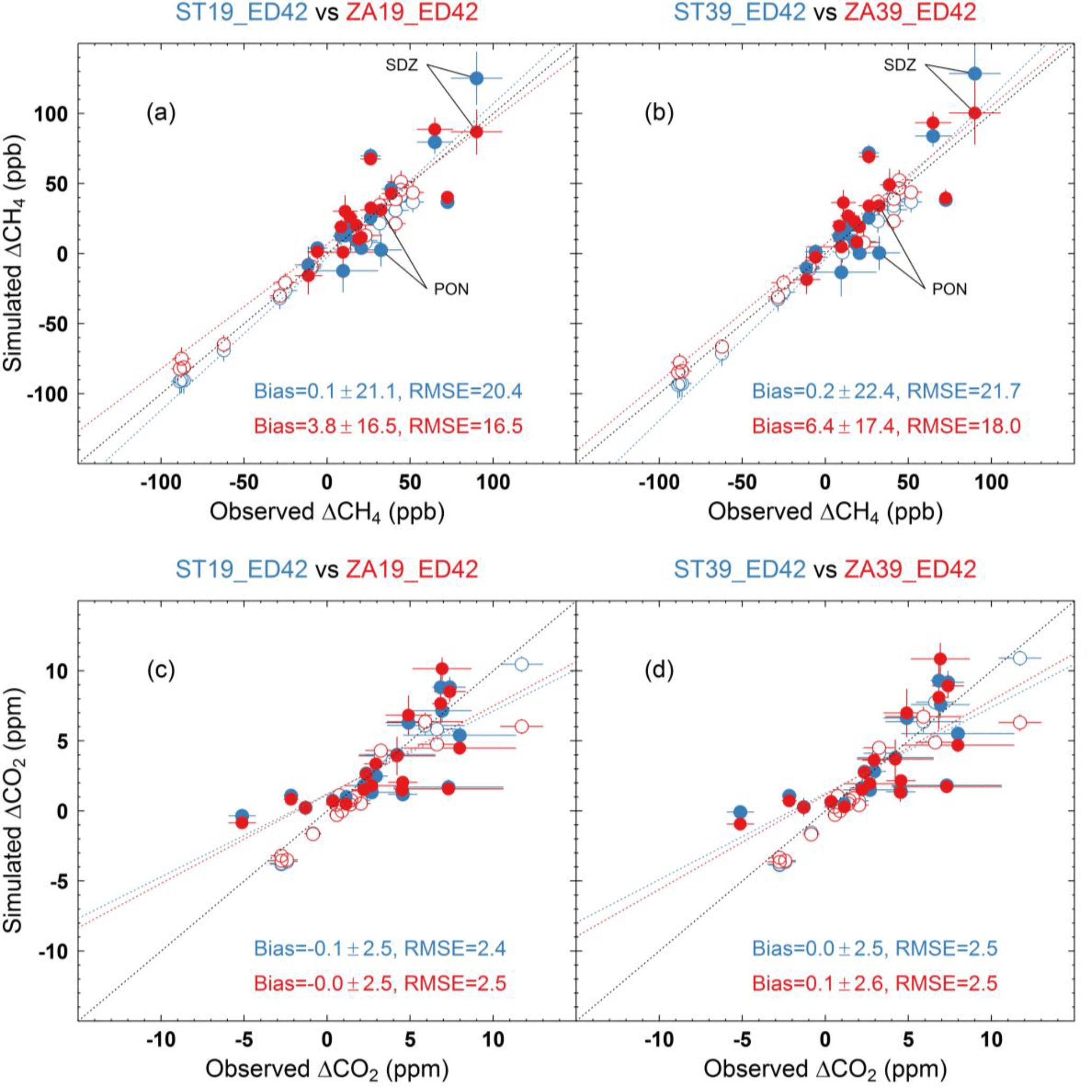
Figure 2 Scatterplots of the simulated and observed mean annual gradients of CH₄ (a, b) and CO₂ (c, d) between HLE and other stations. In each panel, the simulated CH₄ or CO₂ gradients are based on model outputs from STs (blue circles) and ZAs (red circles), respectively. The black dotted line indicates the identity line, whereas the blue and red dotted lines indicate the corresponding linear fitted lines. The closed and open circles represent stations inside and outside the zoomed region.

When looking into the model performance for different station types, ZAs generally better capture the gradients at coastal and continental stations within the zoomed region, given the substantial reduction of RMSE compared to STs (Table S1). For example, significant model improvement is found at Shangdianzi (SDZ – 40.65^∘ N, 117.12^∘ E; 293 $\mathrm{m}\mathrm{a}.\mathrm{s}.\mathrm{l}.$) and Pondicherry (PON – 12.01^∘ N, 79.86^∘ E; 30 $\mathrm{m}\mathrm{a}.\mathrm{s}.\mathrm{l}.$) (Fig. 2a and b), with each having an average bias reduction of 28.1 (73.0 %) and 30.3 (94.7 %) ppb respectively compared to STs for the 39-layer model (Table S2). This improvement mainly results from reduction in representation error with higher model horizontal resolutions in the zoomed region through better description of surface fluxes and/or transport around the stations. Particularly, given the presence of large CH₄ emission hotspots within the zoomed region (Fig. S4), ZAs makes the simulated CH₄ fields more heterogeneous around emission hotspots (e.g., North China in Fig. S5), having the potential to better represent stations nearby on an annual basis if the surface fluxes are prescribed with sufficient accuracy.

However, finer resolutions may enhance model–data misfits due to inaccurate meteorological forcings and/or surface flux maps. For example, for the coastal station Tae-ahn Peninsula (TAP – 36.73^∘ N, 126.13^∘ E; 21 $\mathrm{m}\mathrm{a}.\mathrm{s}.\mathrm{l}.$) with significant emission sources nearby (Fig. S6), both ZAs and STs overestimate the observed CH₄ gradients by $>+$15 ppb, and ZA39 perform even worse than other versions (Table S2). The poor model performance at TAP suggests that the prescribed emission sources are probably overestimated within the station's footprint area (also see the marine station GSN, Fig. S6), and higher model resolutions (whether in horizontal or in vertical) tend to inflate the model–observation misfits in this case. In addition, as stated in several previous studies (Geels et al., 2007; Law et al., 2008; Patra et al., 2008), for a station located in a complex terrain (e.g., coastal or mountain sites), the selection of an appropriate grid point and/or model level to represent an observation is challenging. In this study we sample the grid point and model level nearest to the location of the station, which may not be the best representation of the data sampling selection strategy (e.g., marine sector at coastal stations) and could contribute to the model–observation misfits.

3.1.2 CO₂ annual gradients

Both ZAs and STs can generally capture the CO₂ annual gradients between stations, although not as well as for CH₄ (Fig. 2c and d). In contrast with CH₄, ZAs do not significantly improve representation of CO₂ gradients for stations within the zoomed region, with the mean bias and RMSE close to those of STs (Table S1b). At a few stations (e.g., TAP, Fig. S8), ZAs even degrade model performance (Table S2b), possibly related to misrepresentation of CO₂ sources in the prescribed surface fluxes and transport effects. Again increasing model vertical resolution does not impact the overall model performance much.

With finer horizontal resolution, the model improvement to represent the annual gradients is more apparent for CH₄ than for CO₂. One of the reasons may point towards the quality of CO₂ surface fluxes, especially natural ones. They are spatially more diffuse than those of CH₄ and temporally more variable in response to weather changes (Parazoo et al., 2008; Wang et al., 2007). Therefore, the regional variations of net ecosystem exchange (NEE) not captured by the terrestrial ecosystem model (e.g., ORCHIDEE in this paper) may explain the worse model performance on the CO₂ annual gradients compared to CH₄ and less apparent model improvement. Further, the spatial resolution of the prescribed surface flux may also account for the difference in model improvement between CO₂ and CH₄ (e.g., the spatial resolution of anthropogenic emissions is 1^∘ for CO₂ and 0.1^∘ for CH₄). Therefore, with the current setup of surface fluxes (Table 1), ZAs are more likely to resolve the spatial heterogeneity of CH₄ fields, and its improvement over STs is more apparent than that for CO₂.

3.2 Seasonal cycles

3.2.1 CH₄ seasonal cycles

The model performance for the seasonal cycle depends on the quality of seasonal surface fluxes, atmospheric transport, and chemistry (for CH₄ only). For CH₄, both ZAs and STs capture the seasonal phases at most stations within the zoomed region very well (Fig. 3a), and model resolutions (in both horizontal and vertical) do not significantly impact the simulated timing of seasonal maximum and minimum. The seasonal phases at Plateau Assy (KZM – 43.25^∘ N, 77.87^∘ E; 2524 $\mathrm{m}\mathrm{a}.\mathrm{s}.\mathrm{l}.$), Waliguan (WLG – 36.28^∘ N, 100.90^∘ E; 3890 $\mathrm{m}\mathrm{a}.\mathrm{s}.\mathrm{l}.$) and Ulaan Uul (UUM – 44.45^∘ N, 111.10^∘ E; 1012 $\mathrm{m}\mathrm{a}.\mathrm{s}.\mathrm{l}.$) are not well represented, which is probably related to unresolved seasonally varying sources around these stations. The sensitivity test simulations prescribed with wetland emissions from ORCHIDEE outputs show much better model–observation agreement in seasonal phases (Fig. S9). For stations outside the zoomed region, the performance of ZAs is not degraded despite the coarser horizontal resolutions (Fig. S10).

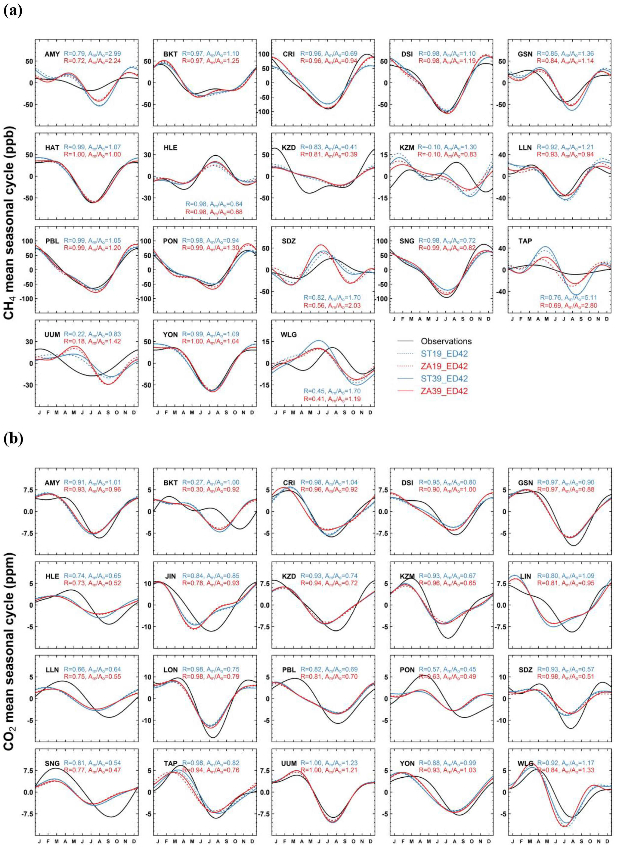
Figure 3 The observed and simulated mean seasonal cycles of CH₄ (a) and CO₂ (b) for stations within the zoomed region. In each panel, the simulated mean seasonal cycles are based on model outputs from STs (blue lines) and ZAs (red lines), respectively. The text shows statistics between the simulated and observed seasonal cycles for 39-layer models.

With respect to the seasonal amplitude, the performance of STs and ZAs shows a significant difference at stations influenced by large emission sources. For example, the seasonal amplitudes of AMY and TAP are strongly overestimated by STs ($A_m/A_o=\mathrm{2.99}$ and $A_m/A_o=\mathrm{5.11}$ for the 39-layer model; Fig. 3a), while ZAs substantially decrease the simulated amplitudes at these two stations with improved model–observation agreement ($A_m/A_o=\mathrm{2.24}$ and $A_m/A_o=\mathrm{2.80}$ for the 39-layer model; Fig. 3a). However, at SDZ the seasonal amplitude is even more exaggerated by ZAs, especially when higher vertical resolution is applied ($A_m/A_o=\mathrm{1.70}$ and $A_m/A_o=\mathrm{2.03}$ for ST39 and ZA39; Fig. 3a). The two contrasting cases suggest that increasing horizontal resolution does not necessarily better represent the CH₄ seasonal cycle, and model improvement or degradation depends on other factors such as accuracy of the temporal and spatial variations of prescribed fluxes, OH fields and meteorological forcings. In addition, as it is found for annual CH₄ gradients, we note that the simulated seasonal amplitudes at stations in East Asia (AMY, TAP, GSN and SDZ) are consistently higher than the observed ones (Fig. 3a), implying that the prescribed CH₄ emissions are probably overestimated in this region.

3.2.2 CO₂ seasonal cycles

The CO₂ seasonal cycle mainly represents the seasonal cycle of NEE from ORCHIDEE convoluted with atmospheric transport. Figure 3b illustrates that both ZAs and STs capture the CO₂ seasonal phases at most stations well, and a high correlation (Pearson correlation R>0.8) between the simulated and observed CO₂ harmonics is found for 14 out of 20 stations within the zoomed region. However, the simulated onset of CO₂ uptake in spring or timing of the seasonal minima tend to be earlier than observations. This shift in phase can be as large as >1 month for several stations (e.g., HLE, JIN and PON in Fig. 3b), yet cannot be reduced by solely refining model resolutions. At BKT in western Indonesia, the shape of the CO₂ seasonality is not well captured (R=0.27 and R=0.30 for ST39 and ZA39; Fig. 3b). Given that representation of the CH₄ seasonal phase at BKT is very good (R=0.97 for ST39 and ZA39; Fig. 3a), the unsatisfactory model performance for CO₂ suggests inaccurate seasonal variations in the prescribed surface fluxes such as NEE and/or fire emissions. As for CH₄, the performance of ZAs is not degraded outside the zoomed region despite the coarser horizontal resolutions (Fig. S11).

With respect to the CO₂ seasonal amplitude, 10 out of 20 stations within the zoomed region are underestimated by more than 20 %, most of which are mountain and continental stations (Fig. 3b). The underestimation of CO₂ seasonal amplitudes at these stations is probably due to the underestimated carbon uptake in northern midlatitudes by ORCHIDEE, which is the case for most land surface models currently available (Peng et al., 2015). Another reason may be related to the misrepresentation of the CO₂ seasonal rectifier effect (Denning et al., 1995), which means that the covariance between carbon exchange (through photosynthesis and respiration) and vertical mixing may not be well captured in our simulations even with finer model resolutions.

3.3 Synoptic variability

3.3.1 CH₄ synoptic variability

The day-to-day variability of CH₄ and CO₂ residuals are influenced by the regional distribution of fluxes and atmospheric transport at the synoptic scale. For CH₄, as shown in Fig. 4a, both STs and ZAs capture the phases of synoptic variability at most stations within the zoomed region fairly well, with 15 out of 18 stations showing model–observation correlation r>0.3. Increasing horizontal resolution can more or less impact model performance, yet the direction of change is station dependent. In general, ZAs improve correlation in phases for most marine and coastal stations compared to STs (e.g., CRI and HAT; Fig. 4a), while degradation in model performance is mostly found for mountain and continental stations (e.g., KZM and SDZ; Fig. 4a). With increased horizontal resolution, better characterization of the phases would require accurate representation of short-term variability in both meteorological forcings and emission sources at fine scales. This presents great challenges on data quality of boundary conditions, especially for mountain stations located in complex terrains or continental stations surrounded by highly heterogeneous yet uncertain emission sources.

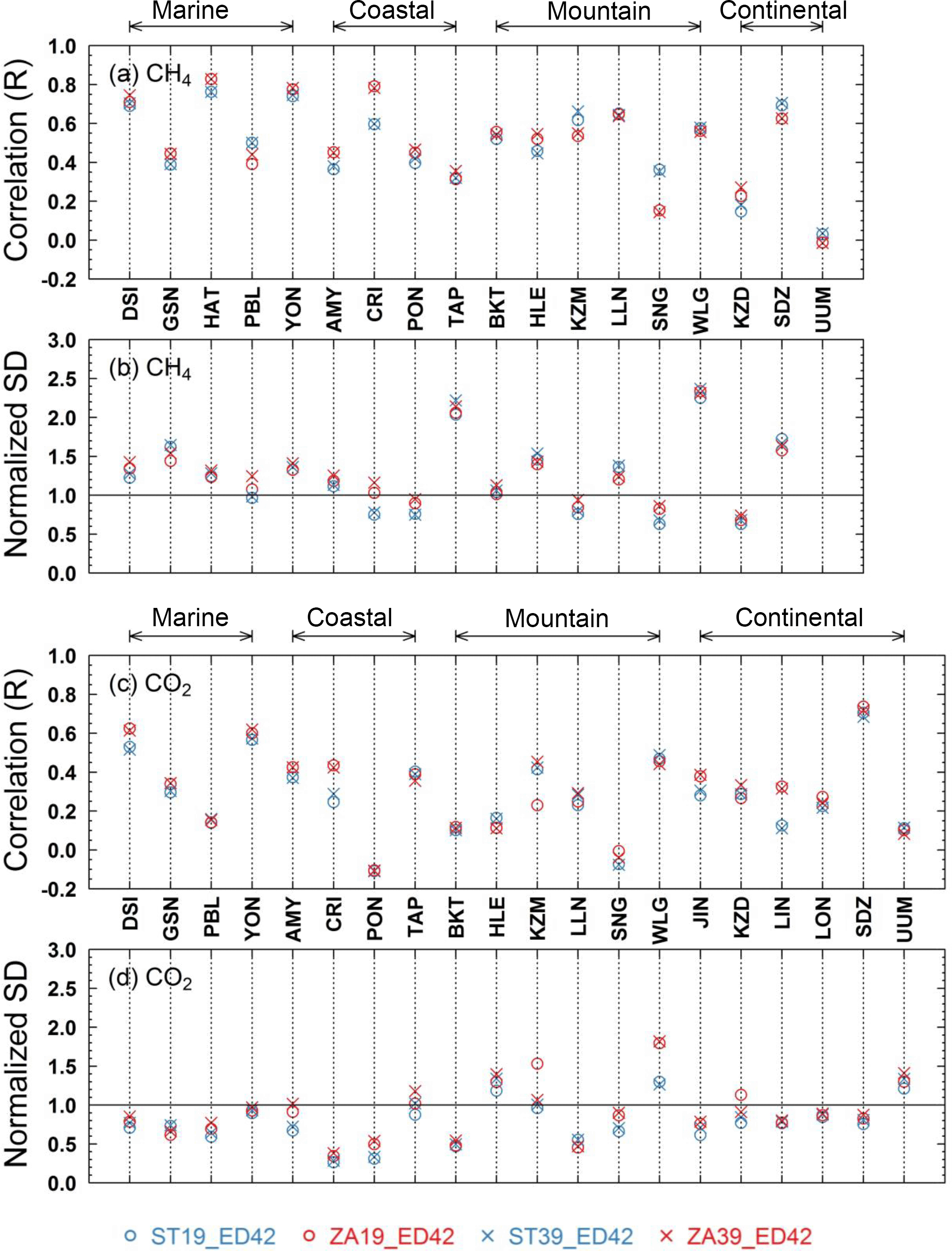
Figure 4 The correlations and normalized SDs between the simulated and observed synoptic variability for CH₄ (a, b) and CO₂ (c, d) at stations within the zoomed region. For each station, the synoptic variability is calculated from residuals from the smoothed fitting curve.

Regarding the amplitudes of CH₄ synoptic variability, 12 out of 18 stations have NSDs within the range of 0.6–1.5, and ZAs generally give higher NSD values than STs for most of these stations (Fig. 4b). For stations with NSDs >1.5, ZAs tend to simulate smaller amplitudes and slightly improve model performance (e.g., GSN, HLE and SDZ; Fig. 4b). One exception is UUM. Given the presence of a wrong emission hotspot near the station in the EDGARv4.2FT2010 dataset (Fig. S6), ZAs greatly inflate the model–observation misfits (Fig. S13). The sensitivity test simulations prescribed with an improved data version EDGARv4.3.2 show much better agreement with observations, although the simulated amplitudes are still too high (Fig. S13). In addition, it is interesting to note that stations in East Asia generally have NSDs >1.5 (e.g., GSN, TAP, SDZ and UUM; Fig. 4b), again suggesting overestimation of the prescribed CH₄ emissions in this region.

3.3.2 CO₂ synoptic variability

For CO₂, as shown in Fig. 4c and d, 12 out of 20 stations within the zoomed region have model–observation correlation r>0.3, whereas 14 out of 20 stations have NSDs within the range of 0.5–1.5. With finer model resolution, significant model improvement (whether regarding phases or amplitudes of CO₂ synoptic variability) is mostly found at marine, coastal and continental stations (e.g., AMY, DSI and SDZ; Fig. 4c and d); for mountain stations, on the contrary, phase correlation is not improved and representation of amplitudes is even degraded (e.g., HLE, LLN and WLG; Fig. 4c and d). As mentioned above for CH₄ synoptic variability, the model degradation at mountain stations may arise from errors in mesoscale meteorology and regional distribution of sources or sinks over complex terrains, probably as well as unresolved vertical processes.

When we examine model performance for CO₂ vs. CH₄ by stations, there are stations at which phases of synoptic variability are satisfactorily captured for CH₄ but not for CO₂ (e.g., BKT, PBL, PON; Fig. 4a and c). At PON, a tropical station on the southeast coast of India, the simulated CO₂ synoptic variability is even out of phase with observations all year around and during different seasons (Fig. S14; Table S3). The poor model performance should be largely attributed to the imperfect prescribed CO₂ surface fluxes. As noted by several previous studies (e.g., Patra et al., 2008), CO₂ fluxes with sufficient accuracy and resolution are indispensable for realistic simulation of CO₂ synoptic variability. In this study, the daily to hourly NEE variability does not seem to be well represented in ORCHIDEE, especially in the tropics. Further, for stations influenced by large fire emissions (e.g., BKT), using the monthly averaged biomass burning emissions may not be able to realistically simulate CO₂ synoptic variability due to episodic biomass burning events. In addition, the prescribed CO₂ ocean fluxes have a rather coarse spatial resolution ($\mathrm{4}{}^{\circ }\times \mathrm{5}{}^{\circ }$), which may additionally account for the poor model performance, especially for marine and coastal stations.

3.4 Diurnal cycle

3.4.1 CH₄ diurnal cycle

The diurnal cycles of trace gases are mainly controlled by the covariations between local surface fluxes and atmospheric transport. To illustrate model performance on diurnal cycles, we take a few stations with continuous measurements as examples. For CH₄, as shown in Fig. 5a, the mean diurnal cycles can be reasonably well represented at the marine/coastal stations GSN and PON for the specific study periods (also see Table S4), although monthly fluxes are used to prescribe the models. Compared to STs, the diurnal cycles simulated by ZAs agree much better with observations (Fig. 5a), which is possibly due to more realistic representation of coastal topography, land–sea breeze, and/or source distribution at finer grids. However, there are also periods during which the CH₄ diurnal cycles are not satisfactorily represented by both model versions or model performance is degraded with higher horizontal and/or vertical resolutions (Table S4). The model–observation mismatch may be due to the following reasons. First, the prescribed monthly surface fluxes are probably not adequate to resolve the short-term variability at stations strongly influenced by local and regional sources, especially during the seasons when emissions from wetlands and rice paddies are active and temporally variable with temperature and moisture. Second, the sub-grid scale parameterizations in the current model we used are not able to realistically simulate the diurnal cycles of boundary layer mixing. Recently new physical parameterizations have been implemented in LMDz to better simulate vertical diffusion and mesoscale mixing by thermal plumes in the boundary layer (Hourdin et al., 2002; Rio et al., 2008), which can significantly improve simulation of the daily peak values during nighttime and thus diurnal cycles of tracer concentrations (Locatelli et al., 2015a).

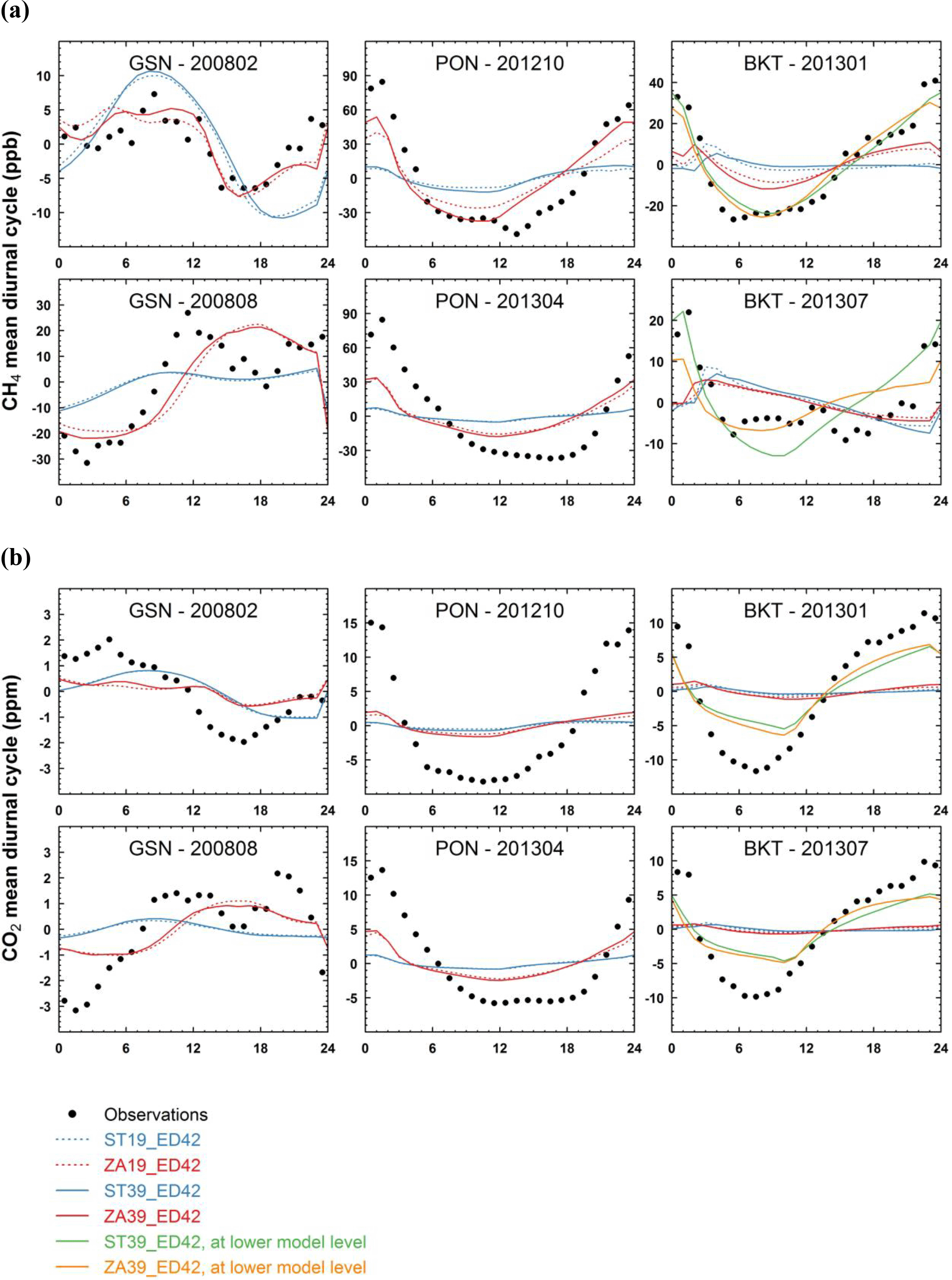
Figure 5 The observed and simulated mean diurnal cycles (in UTC time) of CH₄ (a) and CO₂ (b) at three stations within the zoomed region. For BKT, the simulated diurnal cycles at lower model levels are also presented.

Representation of the CH₄ diurnal cycle at mountain stations can be even more complicated, given that the mesoscale atmospheric transports such as mountain-valley circulations and terrain-induced up-down slope circulations cannot be resolved in global transport models (Griffiths et al., 2014; Pérez-Landa et al., 2007; Pillai et al., 2011). At BKT, a mountain station located on an altitude of 869 $\mathrm{m}\mathrm{a}.\mathrm{s}.\mathrm{l}.$, the CH₄ diurnal cycle is not reasonably represented when model outputs are sampled at the levels corresponding to this altitude (level 3 and level 4 for 19-layer and 39-layer models). The simulated CH₄ diurnal cycles sampled at a lower model level (level 2 for both 19-layer and 39-layer models) agree much better with the observed ones (Fig. 5a). This suggests that the current model in use is not able to resolve mesoscale circulations in complex terrains, even with the zoomed grids (∼50 km over the focal area) and 39 model layers.

3.4.2 CO₂ diurnal cycle

For CO₂, as shown in Fig. 5b, the simulated diurnal cycles at GSN and PON correlate fairly well with the observed ones for their specific study periods (also see Table S5). The amplitudes of diurnal cycles are greatly underestimated, although this can be more or less improved with finer horizontal resolutions (Fig. 5b). As for CH₄, the model–observation discrepancies mainly result from underestimated NEE diurnal cycles from ORCHIDEE and/or unresolved processes in the planetary boundary layer. Particularly, neither ZAs nor STs are able to adequately capture the CO₂ diurnal rectifier effect (Denning et al., 1996). For stations strongly influenced by local fossil fuel emissions, underestimation of the amplitudes may be additionally attributed to fine-scale sources not resolved at current horizontal resolutions. This is the case for PON, a coastal station 8 km north of the city of Pondicherry in India with a population of around 750 000 (Lin et al., 2015), where the amplitudes of diurnal cycles are underestimated for both CO₂ and CH₄ (Fig. 5a and b). Again at BKT, as noted for CH₄, a better model–observation agreement is found for the CO₂ diurnal cycle when model outputs are sampled at the surface layer rather than the one corresponding to the station altitude (Fig. 5b). Note that even the simulated diurnal cycles at the surface level are smaller compared to the observed ones by ∼50 %, suggesting that the diurnal variations of both NEE fluxes and terrain-induced circulations are probably not satisfactorily represented in the current simulations.

3.5 Evaluation against the CONTRAIL CO₂ vertical profiles

Figure 6 shows the simulated and observed CO₂ vertical profiles averaged for different seasons and over different regions. Over East Asia (EAS; Figs. 6a and S1), both ZAs and STs reasonably reproduce the shape of the observed CO₂ vertical profiles above 2 km, while below 2 km the magnitude of ΔCO₂ is significantly underestimated by up to 5 ppm. The simulated CO₂ vertical gradients between the planetary boundary layer (BL) and free troposphere (FT) are lower than the observations by 2–3 ppm during winter (Fig. 7a). The model–observation discrepancies are possibly due to stronger vertical mixing in LMDz (Locatelli et al., 2015a; Patra et al., 2011) as well as flux uncertainty. Note that, as most samples (79 %) are taken over the Narita International Airport (NRT) and Chubu Centrair International Airport (NGO) in Japan located outside the zoomed region (Fig. S1), STs capture the BL–FT gradients slightly better than ZAs.

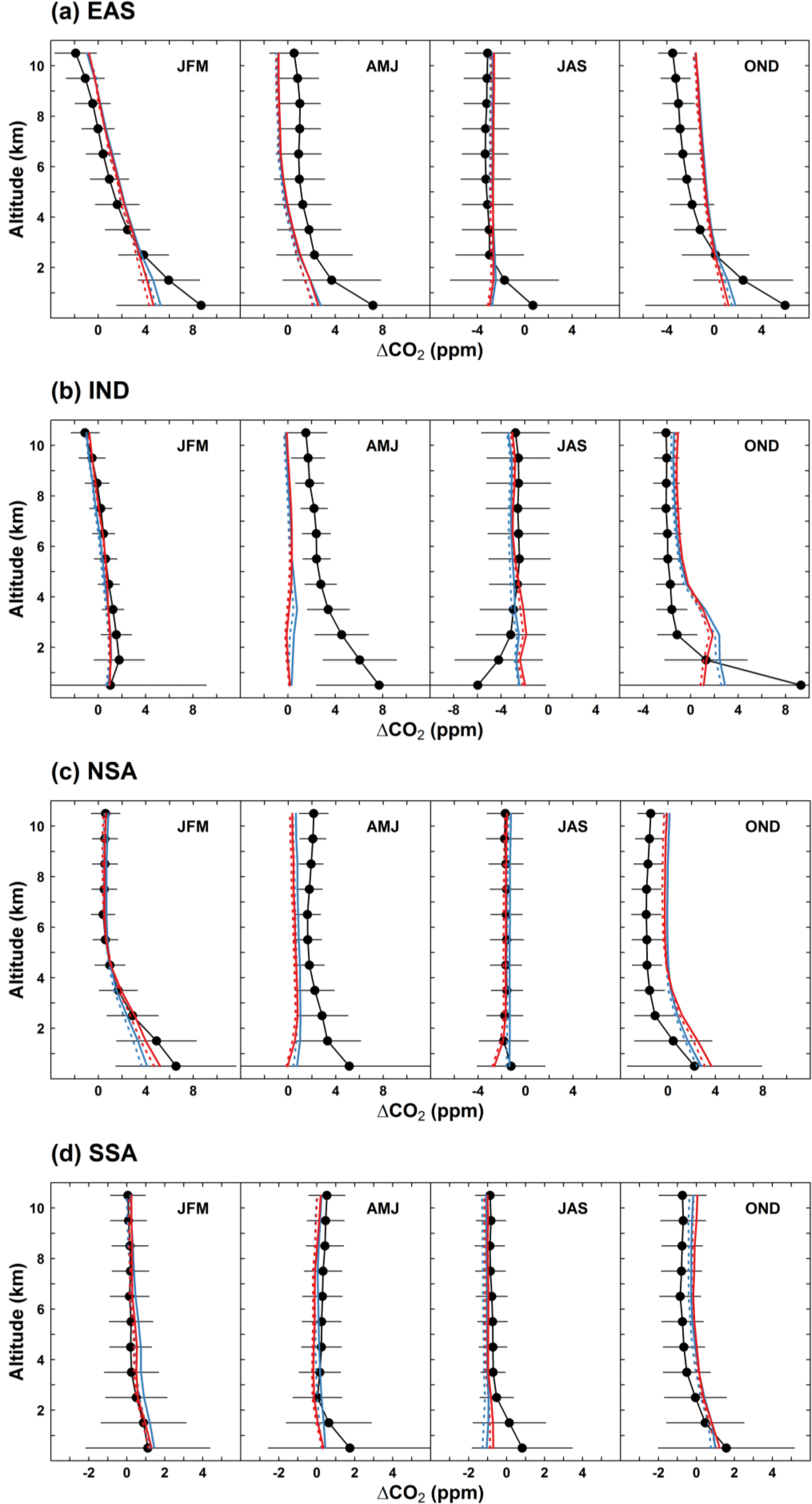
Figure 6 Seasonal mean observed and simulated CO₂ vertical profiles over (a) East Asia (EAS), (b) the Indian subcontinent (IND), (c) northern Southeast Asia (NSA) and (d) southern Southeast Asia (SSA). The observed vertical profiles are based on CO₂ continuous measurements onboard the commercial flights from the CONTRAIL project during the period 2006–2011. For each 1 km altitude bin and each subregion, the observed and simulated time series are detrended (denoted as ΔCO₂) and seasonally averaged during January–March (JFM), April–June (AMJ), July–September (JAS) and October–December (OND).

Over the Indian subcontinent (IND, Fig. 6b), there is large underestimation of the magnitude of ΔCO₂ near the surface by up to 8 ppm during April–June (AMJ), July–September (JAS) and October–December (OND). Accordingly, the BL–FT gradients are also underestimated by up to 3–4 ppm for these periods (Fig. 7b). The model–observation discrepancies are probably due to vertical mixing processes not realistically simulated in the current model (including deep convection), as well as the imperfect representation of CO₂ surface fluxes strongly influenced by the Indian monsoon system.

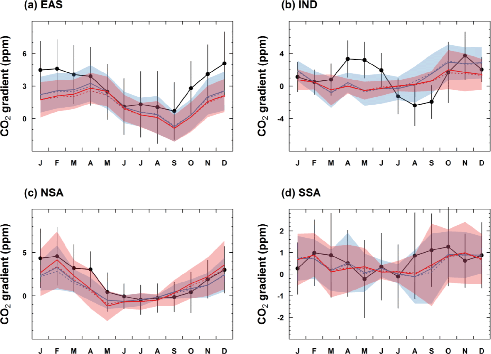
Figure 7 Monthly mean observed and simulated CO₂ gradient between 1 and 4 km over (a) East Asia (EAS), (b) the Indian subcontinent (IND), (c) northern Southeast Asia (NSA) and (d) southern Southeast Asia (SSA). For each subregion, the monthly CO₂ gradients are calculated by averaging the differences in CO₂ concentrations between 1 and 4 km over all the vertical profiles.

The CO₂ vertical profiles over Southeast Asia (including northern Southeast Asia and southern Southeast Asia) are generally well reproduced (Fig. 6c and d). However, both ZAs and STs fail to reproduce the BL–FT gradient of ∼3 ppm in April for NSA (Fig. 7c). Apart from errors due to vertical transport and/or prescribed NEE, inaccurate estimates of biomass burning emissions could also contribute to this model–observation mismatch.

Overall, the CO₂ vertical profiles in free troposphere are well simulated by both STs and ZAs over SEA, while significant underestimation of the BL–FT gradients is found for East Asia and the Indian subcontinent. The model–observation mismatch is due to misrepresentation of both vertical transport and prescribed surface fluxes and can not be significantly reduced by solely refining the horizontal and/or vertical resolution, as shown by the very similar CO₂ vertical profiles simulated from ZAs and STs. New physical parameterization as shown in Locatelli et al. (2015a) should be implemented in the model to assess its potential to improve simulation of the vertical profiles of trace gases (especially the BL–FT gradients).

4 Conclusions and implications

In this study, we assess the capability of a global transport model (LMDz-INCA) to simulate CH₄ and CO₂ variabilities over South and East Asia (SEA). Simulations have been performed with configurations of different horizontal (standard vs. Asian zoom) and vertical (19 vs. 39) resolutions. Model performance to represent trace gas variabilities is evaluated for each model version at multi-annual, seasonal, synoptic and diurnal scales, against flask and continuous measurements from a unique dataset of 39 global and regional stations inside and outside the zoomed region. The evaluation at multiple temporal scales and comparisons between different model resolutions and trace gases have informed us of both advantages and challenges relating to high-resolution transport modeling. Main conclusions and implications for possible model improvement and inverse modeling are summarized as follows.

First, ZAs improve the overall representation of CH₄ annual gradients between stations in SEA, with reduction of RMSE by 16–20 % compared to STs. The model improvement mainly results from reduction in representation error with finer horizontal resolutions over SEA through better characterization of CH₄ surface fluxes, transport and/or topography around stations. Particularly, the scattered distributed CH₄ emission sources (especially emission hotspots) can be more precisely defined with the Asian zoom grids, which makes the simulated concentration fields more heterogeneous, having the potential to improve representation of stations nearby on an annual basis.

However, as the model resolution increases, the simulated CH₄ concentration fields are more sensitive to possible errors in boundary conditions. Thus, the performance of ZAs at a specific station as compared to STs depends on the accuracy and data quality of meteorological forcings and/or surface fluxes, especially when we examine short-term variabilities (synoptic and diurnal variations) or stations influenced by significant emission sources around. One example is UUM, at which ZAs even greatly degrade representation of synoptic variability due to the presence of a wrong emission hotspot near the station in the EDGARv4.2FT2010 dataset. A sensitivity test prescribed with the improved emission dataset EDGARv4.3.2 shows much better agreement with observations. This emphasizes the importance of accurate a priori CH₄ surface fluxes in high-resolution transport modeling and inversions, particularly regarding locations and magnitudes of emission hotspots. Any unrealistic emission hotspot close to a station (as shown for UUM) should be corrected before inversions, otherwise the inverted surface fluxes are likely to be strongly biased. Moreover, as current bottom-up estimates of CH₄ sources and sinks still suffer from large uncertainties at fine scales, caution should be taken when one attempts to assimilate observations not realistically simulated by the high-resolution transport model. These observations should be either removed from inversions or allocated with large uncertainties.

With respect to CO₂, model performance and the limited model improvement with finer grids suggest that the CO₂ surface fluxes have not been prescribed with sufficient accuracy and resolution. One major component is NEE simulated from the terrestrial ecosystem model ORCHIDEE. For example, the smaller CO₂ seasonal amplitudes simulated at most inland stations in SEA mainly result from underestimated carbon uptake in northern midlatitudes by ORCHIDEE, while the misrepresentation of synoptic and diurnal variabilities (especially for tropical stations like BKT and PON) is related to the inability of ORCHIDEE to satisfactorily capture sub-monthly to daily profiles of NEE. More efforts should be made to improve the simulation of carbon exchange between land surface and atmosphere at various spatial and temporal scales.

Furthermore, apart from data quality of the prescribed surface fluxes, representation of the CH₄ and CO₂ short-term variabilities is also limited by model's ability to simulate boundary layer mixing and mesoscale transport in complex terrains. The recent implementation of new sub-grid physical parameterizations in LMDz is able to significantly improve simulation of the daily maximum during nighttime and thus diurnal cycles of tracer concentrations (Locatelli et al., 2015a). To fully take advantage of high-frequency CH₄ or CO₂ observations at stations close to source regions, the implementation of the new boundary layer physics in the current transport model is highly recommended, in addition to refinement of model horizontal and vertical resolutions. The current transport model with old planetary boundary physics is not capable of capturing diurnal variations at continental or mountain stations; therefore, only observations that are well represented should be selected and kept for inversions (e.g., afternoon measurements for continental stations and nighttime measurements for mountain stations).

Lastly, the model–observation comparisons at multiple temporal scales can give us information about the magnitude of sources and sinks in the studied region. For example, at GSN, TAP and SDZ, all of which are located in East and Northeast Asia, the CH₄ annual gradients as well as the amplitudes of seasonal and synoptic variability are consistently overestimated, suggesting overestimation of CH₄ emissions in East Asia. Therefore atmospheric inversions that assimilate information from these stations are expected to decrease emissions in East Asia, which agree with several recent global or regional studies from independent inventories (e.g., Peng et al., 2016) or inverse modeling (Bergamaschi et al., 2013; Bruhwiler et al., 2014; Thompson et al., 2015). Further studies are needed in the future to estimate CH₄ budgets in SEA by utilizing high-resolution transport models that are capable of representing regional networks of atmospheric observations.