the Creative Commons Attribution 4.0 License.
the Creative Commons Attribution 4.0 License.
 | 03 Jul 2018
Morphological features and mixing states of soot-containing particles in the marine boundary layer over the Indian and Southern oceans
Keiichiro Hara
Masanori Yabuki
Fuminori Hashihama
Jota Kanda
Mixing states of soot-containing aerosol particles constitute important information for the simulation of climatic effects of black carbon in the atmosphere. To elucidate the mixing states and morphological features of soot-containing particles over remote oceans, we conducted on-board observations over the southern Indian Ocean and the Southern Ocean during the TR/V Umitaka-maru UM-08-09 cruise, which started from Benoa, Indonesia, on 1 December 2008 via Cape Town, South Africa, and which terminated in Fremantle, Australia, on 6 February 2009. The light absorption coefficients of size-segregated particles (< 0.5 and < 1.0 µm diameter) and aerosol number concentrations (0.1–0.5 µm diameter) were measured to assist direct aerosol sampling. Size-segregated aerosol particles were collected for chemical analysis using ion chromatography. For transmission electron microscopy (TEM) analyses using water-dialysis methods, dried submicrometer aerosol particles were collected using a cascade impactor. We analyzed 13 TEM samples. Results of water-dialysis analysis demonstrate that most particles were water-soluble. However, for all TEM samples, particles were rarely found (2.1 % of particles on a TEM sample at a maximum) containing insoluble residuals with the characteristic soot shape. For samples collected over the Indian and Southern oceans at latitudes less than 62∘ S, some (20–35 %) soot-containing particles were found as bare soot. For samples collected near the Antarctic coast (65–68∘ S, 38–68∘ E), all soot-containing particles were mixed with water-soluble materials. Furthermore, 56 % of soot-containing particles had a satellite structure formed by the impact of droplets such as sulfuric acid. Chemical analysis of submicrometer particles near the Antarctic coast revealed high concentrations of non-sea-salt (nss) and , suggesting that aged soot-containing particles were transformed by soluble materials derived from dimethyl sulfide (DMS) oxidation. The obtained information of soot at various remote ocean areas is expected to be useful to understand long-range transport processes and to improve simulations of global soot concentration.
- Article
(6028 KB) - Full-text XML
- BibTeX
- EndNote


Soot in the atmospheric aerosol is a by-product of fossil fuel (diesel and coal) combustion and open biomass burning. It is a carbonaceous material with a deep black appearance to visible solar radiation in the atmosphere (Ramanathan and Carmichael, 2008). Soot has an aggregated morphology of globules with diameters of tens of nanometers, consisting of concentrically wrapped graphitic layers (e.g., Pósfai et al., 2004; Murr and Soto, 2005). Carbonaceous materials with a deep black appearance with a large imaginary part of the refractive index are measured optically as black carbon (BC). Although the carbon fractions that are designated by different definitions are far from being the same, those for soot and BC overlap to a great extent (Gelencsér, 2004).
In fact, BC in atmospheric aerosols can influence the Earth's radiation budget strongly through atmospheric processes, but also through positive feedback on snow and ice albedo after transport and deposition on the snow surface at midlatitudes to high latitudes (e.g., Haywood and Boucher, 2000; Hansen and Nazarenco, 2004; Koch and Hansen, 2005; Ramanathan and Carmichael, 2008; Bond et al., 2013). Nevertheless, there are order-of-magnitude disagreements of BC concentrations between models and observations in the remote and upper troposphere air masses (Koch et al., 2009; Schwarz et al., 2010, 2013).
Soot particles that are freshly emitted from fossil fuel combustion are attached to or coated with secondary aerosol materials such as sulfates, nitrates, and organics through atmospheric aging processes (Weingartner et al., 1997; Zuberi et al., 2005). The aging processes alter the particle size, hygroscopicity, and the ability to act as cloud condensation nuclei, eventually reducing the residence time of soot particles in the atmosphere. Some numerical sensitivity studies have pointed out that aging and wet scavenging parameters of soot in the atmosphere are key factors controlling long-range transport and spatial distributions (Koch, 2001; Croft et al., 2005; Stier et al., 2006).
To improve global BC modeling, fundamental information related to aging levels of soot-containing particles is necessary for the atmosphere in remote or polar regions because of their importance for snow albedo effects caused by BC deposition onto snow or sheet ice. Some reports have described aged soot-containing particles using electron microscopy (Pósfai et al., 1999; Hasegawa and Ohta, 2002; Hara et al., 2003; Vester et al., 2007; Ueda et al., 2011b, 2016b; Adachi et al., 2014). However, most of such observations have been limited to sampling locations near source areas. Particularly, knowledge of individual features of soot-containing particles in remote areas of the Southern Hemisphere remains very poor. Although some reports of observations have described BC concentrations over marine boundary layers of the Southern Hemisphere (Moorthy et al., 2005; Evangelista et al., 2007; Sciare et al., 2009) and Antarctica (Wolff and Cachier,, 1998; Hansen et al., 2001; Hara et al., 2008; Chaubey et al., 2010; Weller et al., 2013), information related to mixing states of soot has scarcely been shown.
An important reason for the scarcity of data in remote regions is the difficulty of sampling aerosols under clean conditions. In remote areas, the BC concentration is usually quite low. Moreover, the mass proportion is very low compared to other aerosol components such as sea salt and sulfates. Therefore, it is difficult to find rare soot particles in many other components, particularly well-aged soot. However, water dialysis to detect insoluble soot selectively under a microscope is a powerful technique to investigate the mixing states of well-aged soot-containing particles (Okada, 1983; Ueda et al., 2011a, b). This method comprises morphological observation and comparison before and after water dialysis of aerosols. Because soot shows distinctive morphological features and because it is water-insoluble, this method is suitable to detect soot and to investigate the mixing states with water-soluble materials.
For this study, we conducted careful sampling for individual analysis of soot-containing particles on board the TR/V Umitaka-maru cruises from 1 December 2008 to 6 February 2009 over the southern Indian Ocean and the Southern Ocean. Elucidating the mixing states of soot-containing particles for low-BC concentration areas will be helpful for elucidating the long-range transport of soot in remote areas, and eventually for understanding the global diffusion processes of BC through the atmosphere. This study was conducted mainly to ascertain the mixing states of soot-containing particles with water-soluble materials and to assess their relationship to the morphological features of the mixing materials.
Atmospheric observations were conducted over the Indian Ocean and the Southern Ocean during the TR/V Umitaka-maru UM-08-09 from 1 December 2008 through 6 February 2009. Figure 1 portrays ship tracks of the TR/V Umitaka-maru cruise.
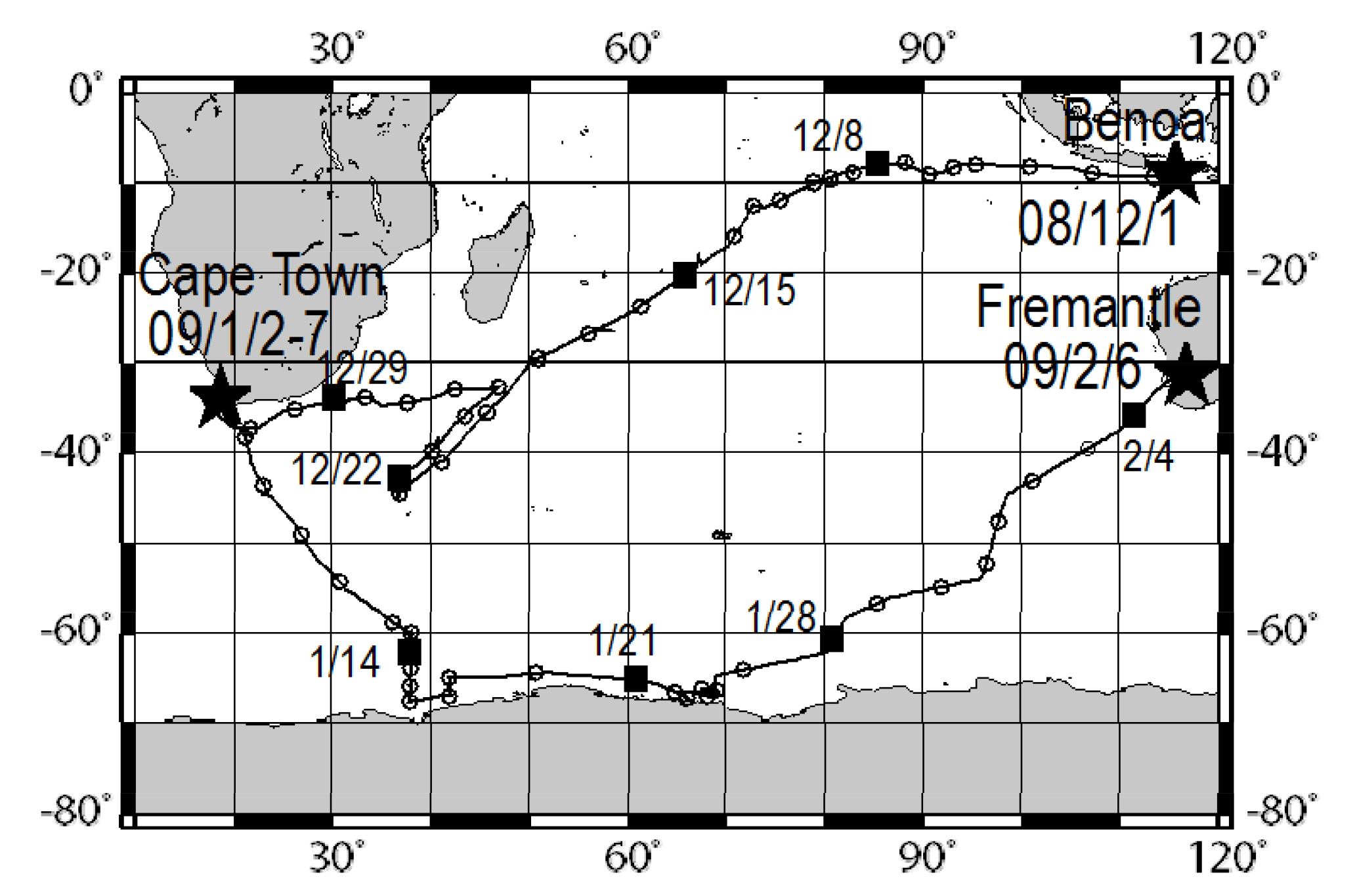
Figure 1Ship tracks of the TR/V Umitaka-maru UM-08-09 cruise. Open circles and black squares represent noon of each day at local time.
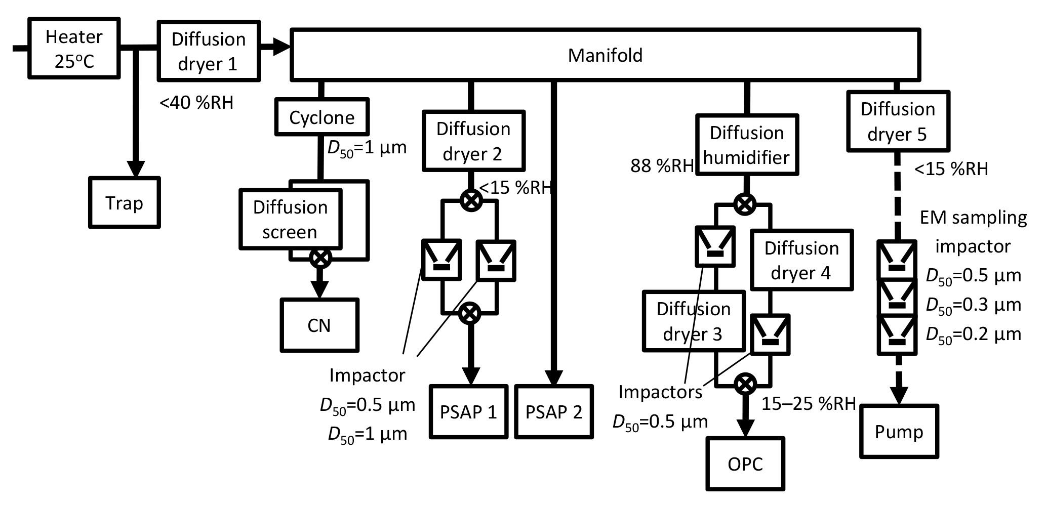
Figure 2Flow diagram of a measurement system using the CN counter, PSAP, and OPC, and a sampling system for TEM samples. Solid arrow lines are sample air flow lines for consecutive measurements. Broken arrow lines show sample air flow for TEM sampling.
2.1 Aerosol number–size distribution
A flow diagram of a measurement system and a sampling system for transmission electron microscopy (TEM) samples is presented in Fig. 2. Number–size distributions of atmospheric aerosol particles were measured using an optical particle counter (OPC, KC-18; Rion Co. Ltd.) similar to the system used for a study described by Ueda et al. (2011a). The OPC measures the number concentrations of aerosol particles for five size ranges, with diameters greater than 0.1, 0.15, 0.2, 0.3, and 0.5 µm. The aerosol measurements were made at relative humidity (RH) of 15–25 %, monitored online using a data logger (MR6600; Chino Corp.).
2.2 Size-segregated light absorption coefficient
Light absorption of aerosol particles was measured using two particle soot absorption photometers (PSAP; Radiance Research), as derived from the particle light absorption coefficient at 565 nm wavelength (babs). The values of babs were corrected based on the method described by Bond et al. (1999). To obtain size information, two impactors (nozzle diameters 0.4 and 1.2 mm, flow rates 0.8 and 1.0 L min−1, respectively) and two two-way valves were used for a PSAP to separate particles with a diameter larger than 0.5 µm and larger than 1 µm. The other was used to measure light absorption for total particles. The valves were changed every 6 min with integration time of 1 min for one photometric value. It is noteworthy that the values of maritime babs, especially those of the larger size range, can be overestimated by the effects of scattering by sea salts and other components on the filter. However, correction of the scattering effect was difficult because babs over the remote ocean region was usually quite low. For this study, values of babs less than 1 µm were used mainly for evaluating the relative variation with attention to overestimation, and as an index of clean sampling of TEM samples aboard the ship.
2.3 Data screening of aerosol number concentration and light absorption
Condensation nuclei (CN) concentrations were measured using a CN counter (3781; TSI) for particles with a diameter greater than 10 nm (Fig. 2). A two-way valve and a diffusion screen to cut particles smaller than 20 nm were used for the CN counter to obtain information about the nucleation particle size. The valves were changed every 10 min. To discuss background aerosol particles specifically, we carefully removed data showing contamination by ship exhaust using CN concentration. As an example, CN concentrations before and after data screening are presented in Fig. 3. CN concentrations before screening sometimes increased dramatically for a short time because of local contamination. We applied restrictions using CN data to the aerosol number–size distribution and babs, and eliminated suspicious data that did not conform to the following: (1) the standard deviation of CN concentrations during 10 min is less than 10 % of the median value and (2) CN concentration during 1 min is lower than 1.2 times the median value for 10 min. As a result of screening according to (1) and (2), periods of rapid CN increase and high CN concentration, which mainly originate from the ship's own emissions, were omitted (Fig. 3). Ueda et al. (2016a) has studied new particle formation over the Pacific Ocean, using a similar screening method. The screening threshold of the rate of increase of the particle number concentration (1.2 times per 10 min) is sufficiently higher than the naturally observed rate of increase for typical new particle formation over the ocean. Therefore, data related to new particle formation would remain after our data screening. For data of OPC and PSAP, only the periods of (1) and (2) were used. Consequently, the aerosol concentration and babs data showed no sudden change, as described later in Sect. 3.1.
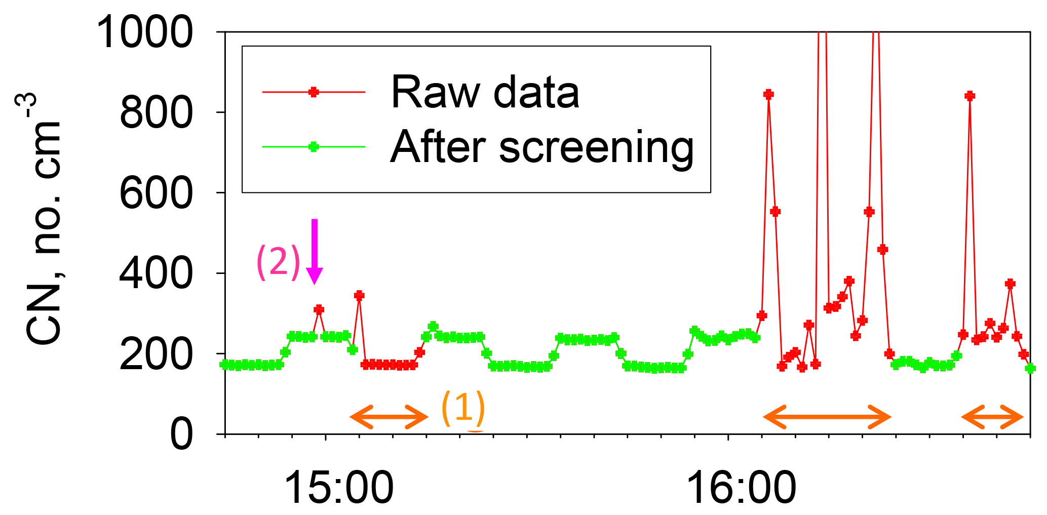
Figure 3Results for CN concentrations measured before and after screening. Data for periods of orange arrows indicate removal by screening (1). Data indicated by pink arrows are data removed by screening (2).
2.4 Ionic constituents of size-segregated aerosol particles
Size-segregated aerosol samples were collected using a three-stage impactor with a backup filter for 24 h intervals at a flow rate of 20 L min−1. The air sampler was placed in a weather shield at the middle of the front end on the uppermost deck. Air sampling was controlled as relative wind speed (> 2 m s−1) and direction (from bow) to avoid contamination from the ship's exhaust. To prevent contamination from the ship's boundary layer, the inlet of the weather shield was designed to protrude toward the bow from the edge of the uppermost deck. A similar arrangement and strategy of aerosol sampling was used by Kawakami et al. (2008). The estimated 50 % cutoff diameter for Stage 1 was 8 µm, with 2 µm for Stage 2, and 0.2 µm for Stage 3 at a flow rate of 20 L min−1. In this study, the Stage 3 results were used for comparison with other aerosol data. The substrate of the first impactor stage was a PTFE filter (47 mm diameter; Advantec Toyo Kaisha Ltd.) with a 15 mm diameter hole at the center. Nuclepore filters (25 mm diameter, 110606; Whatman plc.) were used as sampling substrates for the second and third stages of the impactor. The backup filter was a 47 mm diameter PTFE filter (nominal pore size of 1.0 µm; Advantec Toyo Kaisha Ltd.). These samples were kept in a freezer until laboratory analyses. Filter samples were analyzed using ion chromatography (DX-120; Dionex Corp.) after extraction using 14 mL of ultrapure water (18.2 MΩ). Analytical conditions and procedures were described by Hara et al. (2004).
2.5 Samples of morphological particle analyses using an electron microscope
Aerosol particles were collected for morphological particle analysis using a transmission electron microscope (TEM). To analyze morphological features of aerosol particles, dried (RH < 15 %) aerosols were collected using cascade impactors (50 % cutoff diameters of the three stages 1, 2, and 3 were, respectively, 0.5, 0.3, and 0.2 µm) on carbon-coated nitrocellulose (collodion) films. Aerosol samples were collected for 20–70 min at a flow rate of about 0.6 L min−1. In this study, samples of stages 1 and 2 were used for analyses. To control the suitable surface density of particles on the sampling substrate for observation by TEM analysis, the sampling time was controlled according to aerosol number concentrations. TEM samples were taken at about 2–5 samples per day based on aerosol concentrations and light absorption of aerosol particles. For analysis of atmospheric aerosols, locally contaminated aerosol samples were eliminated by reference to the CN concentration during TEM sample collection from the same inlet tube. The TEM samples were stored under dry conditions at room temperature until TEM analyses were conducted at Nagoya University.
The particles were photographed using TEM (JEM-2010; JEOL) at 2000× magnification. The collection film is regarded to be a semipermeable membrane. Therefore, a water-dialysis technique (Mossop, 1963; Okada, 1983; Okada and Hitzenberger, 2001; Ueda et al., 2011a, b) was applied to aerosol samples to remove water-soluble materials from individual aerosol particles through the film after they were photographed. The electron microscopic grid with particle samples was floated on ultrapure water at room temperature (about 25 ∘C) for 3 h with the collection side facing upward. The water-insoluble residues after dialysis were coated again perpendicularly to the previous coat of a Pt ∕ Pd alloy to differentiate the particle height and two-dimensional morphology after water dialysis. They were then rephotographed using TEM.
The negative films were scanned and recorded with a resolution of 1200 dpi. The scanned image was processed using image analysis software (Win Roof; Mitani Corp.) to estimate the projected area of particles (S). The diameter of the equivalent circle was estimated from S. The mixing states of individual particles with respect to water solubility were obtained by comparing electron micrographs of the same field of the collecting surface taken before and after water dialysis. For morphological analysis using water dialysis, 365–6270 particles per sample were compared before and after water dialysis.
2.6 Air mass backward trajectories
Air mass backward trajectories were analyzed to investigate their relation to observed size distributions and mixing states of aerosol particles. The backward trajectory and precipitation data were computed using the Hybrid Single-Particle Lagrangian Integrated Trajectory (HYSPLIT) model developed by the National Oceanic and Atmospheric Administration (NOAA) Air Resources Laboratory (ARL) (Stein et al., 2015; Rolph et al., 2017). The settings of the trajectory duration, starting height, vertical mode calculation method, and dataset were chosen, respectively, to be 10 days, 500 m above sea level, model vertical velocity, and GDAS meteorological data.
3.1 Temporal variation of aerosol parameters
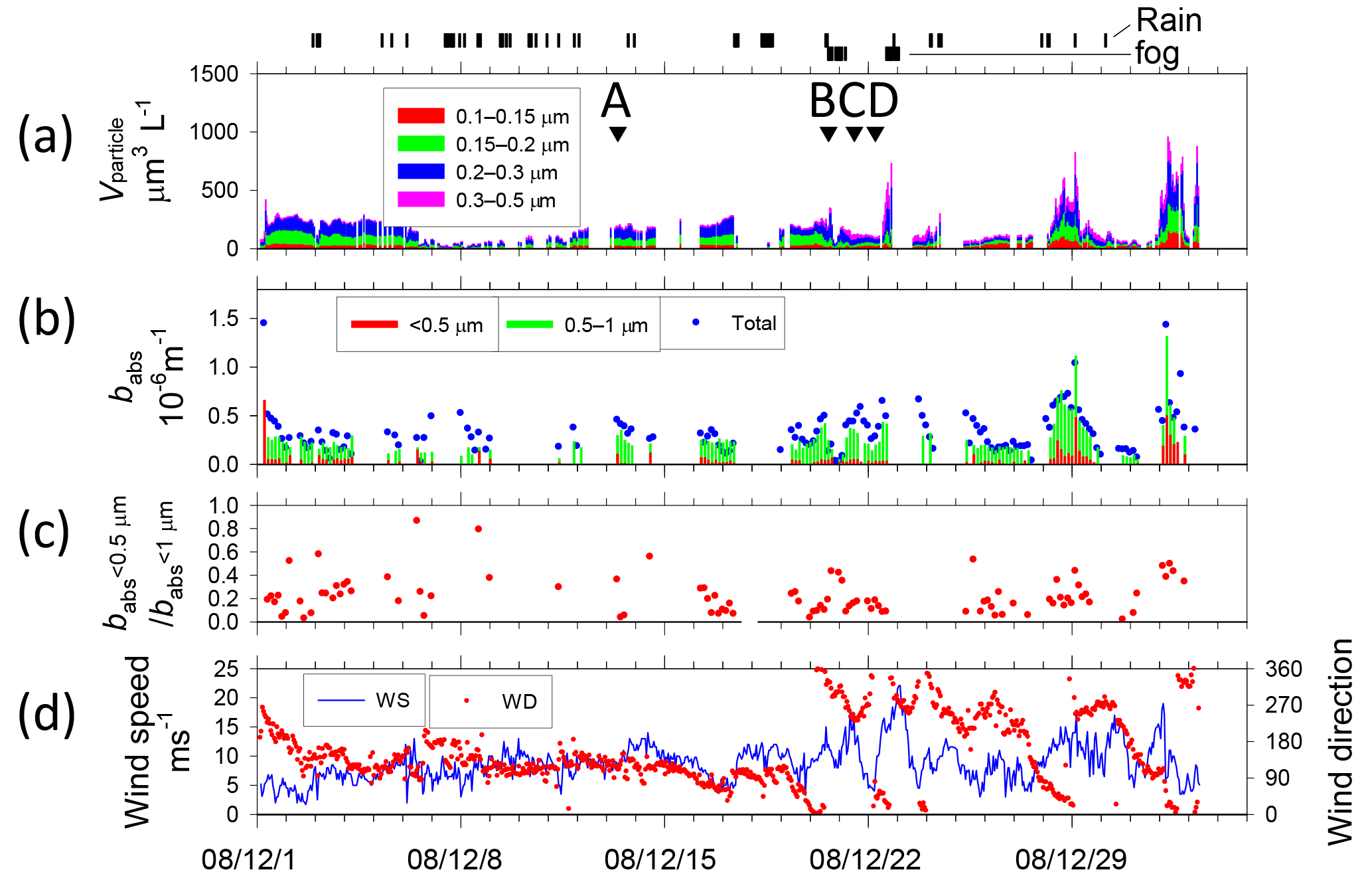
Figure 4Temporal variations of (a) volume concentration of aerosol particles and start times of TEM sampling (A–M with arrows), (b) absorption coefficient babs of size-segregated aerosols, (c) ratio of babs of < 0.5 µm to babs of < 1.0 µm particles, and (d) wind speed and direction from Benoa to Cape Town. Vertical marks above (a) show periods of rain and fog.
Figures 4 and 5 portray temporal variations of the size-segregated volume concentration (0.1–0.5 µm diameter) of aerosol particles (Figs. 4a and 5a), the babs of the size-segregated aerosol particles (D: < 0.5, 0.5–1.0, > 1.0 µm) (Figs. 4b and 5b), the ratio of the babs of D < 0.5 to D < 1.0 µm aerosols (Figs. 4c and 5c), and wind speed and direction (Figs. 4d and 5d), respectively, for Benoa–Cape Town and Cape Town–Fremantle. The volume concentrations were calculated from the number concentrations for the respective size ranges of the OPC and their geometric mean diameters, assuming spherical particles. Contaminated data were removed from the dataset based on the screening method. The fog, rain, and snow periods are shown at the top of Figs. 4a and 5a.
The total volume concentrations of aerosols over remote ocean areas were usually 100–500 µm3 L−1. They were high, about 1000 µm3 L−1, near South Africa (28–29 December 2008, 1–2 and 7–8 January 2009). Throughout the observation period, aerosol volume concentrations of 0.15–0.3 µm diameter comprised about half of the total volume concentration.
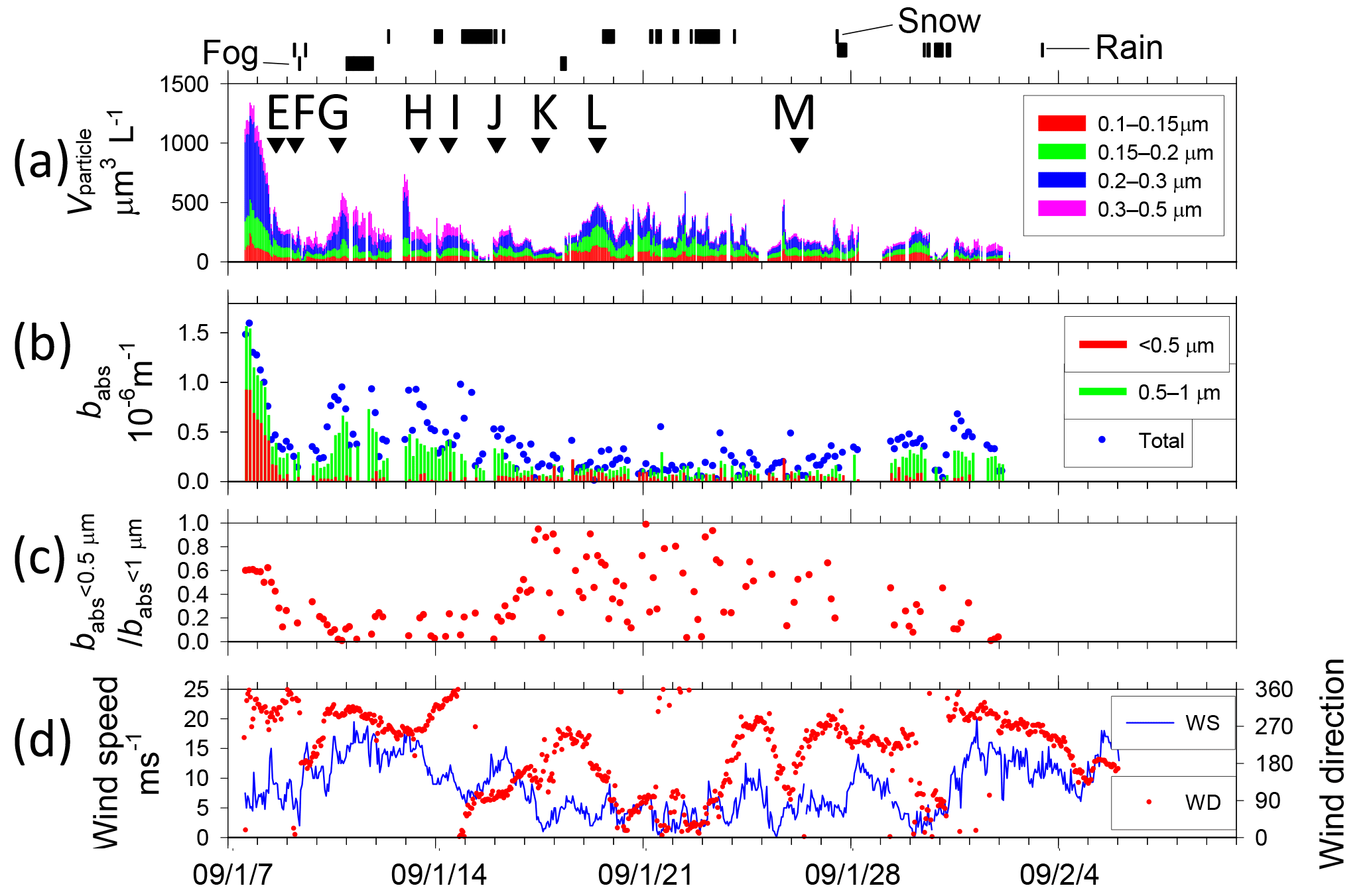
Figure 5Temporal variations of (a) volume concentration of aerosol particles and start times of TEM sampling (A–M with arrows), (b) absorption coefficient babs of size-segregated aerosols, (c) ratio of babs of < 0.5 µm to babs of < 1.0 µm particles, and (d) wind speed and direction from Cape Town to Fremantle. Vertical marks above (a) show periods of snow, rain, and fog.
The highest babs (> 1.0 × 10⁻⁶ m−1 at D < 1 µm particle) was observed near the coast of South Africa (7 January 2009), but babs values soon decreased with distance from the coast. The ratio of 0.5 to 1.0 µm particles also tended to decrease concomitantly with increasing distance from the coast (7–8 January 2009). High values of babs (> 0.4 × 10⁻⁶ m−1 at D < 1 µm particle) were observed on 13 and 20–25 December 2008, 10–11, 13–16, and 28–31 January 2009, and 1 February 2009. Near the Antarctic coast on 16–28 January 2009, babs was mostly approx. 0.1 × 10⁻⁶ m−1 (0.3 × 10⁻⁶ m−1 at most) for D < 1 µm particles. The ratio of 0.5 to 1.0 µm was high. Some observation studies have measured BC concentration over oceans of the Southern Hemisphere (Moorthy et al., 2005; Evangelista et al., 2007; Sciare et al., 2009) based on light absorption measurements. Moorthy et al. (2005) measured a BC value over the Arabian Sea, the tropical Indian Ocean, and the Southern Ocean. The values of BC remained < 50 ng m−3 and remarkably steady (in space and time) in the Southern Ocean (20–56∘ S, 42–60∘ E) during January–March. Evangelista et al. (2007) measured BC values at the southern East Atlantic coast at latitudes of 22–62∘ S. The values of BC at 50–62∘ S were less than 40 ng m−3. Sciare et al. (2009) conducted long-term observations of filter-based monitoring of carbonaceous aerosols at Amsterdam Island (37∘ S, 77∘ E). They reported that BC concentrations were among the lowest reported for a marine atmosphere, with monthly mean levels ranging from 2 to 5 ng C m−3 during summer. Based on light absorption, BC concentrations in Antarctica have been reported from some observation studies (Wolff and Cachier, 1998; Hansen et al., 2001; Hara et al., 2008; Chaubey et al., 2010; Weller et al., 2013). According to those reports, BC concentrations for summer have been reported as 0.5–5.0 ng m−3 at Halley Station (75∘ S, 26∘ E) by Wolff and Cachier (1998), 20–300 ng m−3 at McMurdo Station (78∘ S, 167∘ E) by Hansen et al. (2001), less than 10 ng m−3 at Syowa Station (69∘ S, 39∘ E) by Hara et al. (2008), 4–19 ng m−3 at Larsemann Hills (69∘ S, 77∘ E) and 20–157 ng m−3 at Maritri (70∘ S, 12∘ E) by Chaubey et al. (2010), and approx. 2 ng m−3 monthly median at Neumayer Station (70∘ S, 8∘ W) by Weller et al. (2013). For Maritri, Chaubey et al. (2010) pointed out that the considerable impact of local pollution by human activities must be considered along with results. If a mass-specific absorption cross section of BC was assumed to be 10 m2 g−1 (Hansen et al., 1984; Gelencsér, 2004), then the BC mass concentration in this study was calculated roughly to be > 100 ng m−3 near the coast of South Africa, but usually 20–60 ng m−3 in the remote ocean, showing a similar BC level to those of reports by Moorthy et al. (2005) and by Evangelista et al. (2007). In addition, the calculated BC concentration near Antarctica (65–68∘ S, 38–68∘ E) was about 10 ng m−3 (30 ng m−3 at most), showing a low level similar to data from other reports of coastal areas of Antarctica (McMurdo Station, Syowa Station, Larsemann Hills, and Maritri).
Wind speeds (Fig. 4d) varied during observation periods from 0 to 23 m s−1. High wind speeds (> 15 m s−1) were often observed at latitudes of 40–60∘ S (21–23 December 2008, 11–13 January 2009, and 1 February 2009). Wind speeds over the Southern Ocean near the coast of Antarctica (16–27 January 2009) were mostly lower than 10 m s−1 and were often less than 5 m s−1. The mass concentrations of sea-salt aerosol particles derived from the ocean are known to correlate well with wind speed (Lewis and Schwartz, 2004). Although the aerosol concentrations of D>0.3 µm were often higher under high wind speed conditions (e.g., 22 December 2008), no correlation was found between wind speed and aerosol concentration.
3.2 Relation between backward air mass trajectory and horizontal distribution of absorption coefficient and nss-K+
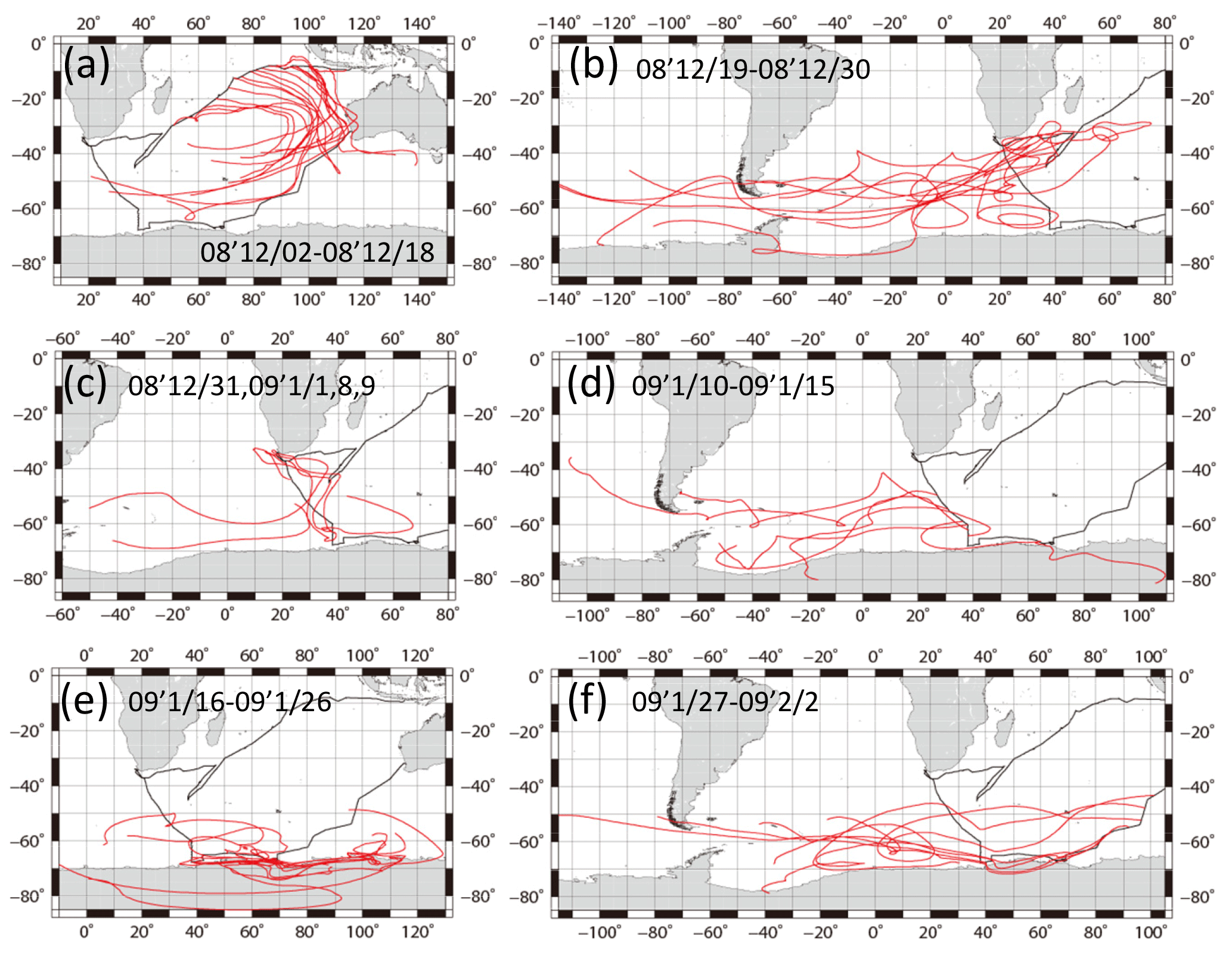
Figure 6The 10-day backward air mass trajectories along the ship tracks. Calculations started from 500 m a.s.l. above the site every day at noon, local time. Red lines show backward air mass trajectories. Black lines show ship tracks.
Figure 6 portrays 10-day backward air mass trajectories. Calculations started from 500 m above sea level over the location at noon, local time, every day. According to starting areas, trajectory analyses were grouped into six zones (Fig. 6a–f). The air masses of the eastern Indian Ocean (2–18 December 2008) were derived from southern subtropical or more southern areas, moving counterclockwise to the observation sites (Fig. 6a). Air masses of the western Indian Ocean (19–30 December 2008, Fig. 6b), south of South Africa of 50–65∘ S (10–15 January 2009, Fig. 6d), and southwest of Australia (27–31 January and 1, 2 February 2009, Fig. 6f) were derived southwest of the Atlantic Ocean. Some of them passed around the area south of South America. The air masses from near the coast of South Africa (31 December 2008, 1, 8, and 9 January 2009, Fig. 6c) passed the coast of South Africa, moving counterclockwise from the south. Air masses from the Southern Ocean near Antarctica (16–26 January 2009, Fig. 6e) originated from the Antarctic coast.
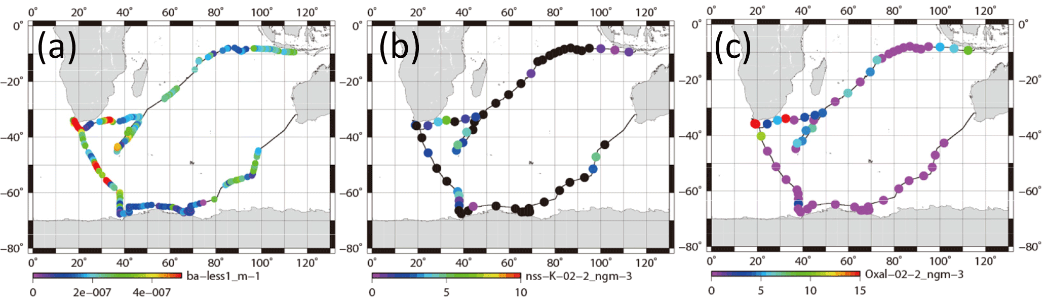
Figure 7Horizontal variation of (a) absorption coefficient of particles smaller than 1 µm, (b) mass concentration of nss-K+ for 0.2–2 µm aerosols, and (c) mass concentration of oxalate for 0.2–2 µm aerosols. Black circles show values below the detection limit.
Figure 7a portrays a horizontal distribution of babs for particles with less than 1.0 µm diameter. The babs around South Africa was higher. High values (> 4 × 10⁻⁷ m−1) were often observed in the western Indian Ocean (35–45∘ S 35–45∘ E on 20–25 December 2008), south of South Africa (50–65∘ S 26–38∘ E on 10–11, 13–16 January 2009), and southwest of Australia (45–63∘ S 80–98∘ E on 28–31 January and 1 February 2009). For these periods, backward air trajectories were mostly derived south of South America. In the subtropical area of South America, biomass burning was often observed by satellite (Edwards et al., 2006; Giglio et al., 2006; Chen et al., 2013). Figure 7b and c respectively portray horizontal distributions of non-sea-salt potassium (nss-K+) and oxalate concentrations in aerosol particles with sizes of 0.2–2 µm. These species are regarded as originating mainly from biomass burning (Andreae, 1983; Kawamura and Kaplan, 1987; Narukawa et al., 1999). Although the nss-K+ concentrations were below the detection limit (black circle in Fig. 7b) in broad remote ocean areas, discernible nss-K+ (> 3 ng m−3) concentrations were observed on 20–23 and 25 December 2008 (western Indian Ocean), on 9 and 12–16 January 2009 (Southern Ocean), and on 31 January and 1 February 2009 (region southwest of Australia). High concentrations (> 5 ng m−3) of oxalate were also observed in the Indian Ocean on 13–14, 19–20, and 22–23 December 2008. Dates of higher concentrations of nss-K+ or oxalate mostly coincided with higher babs. Some reports of observation have described plumes from South America and southern Africa at Syowa Station (Hara et al., 2010) and Troll Research Station (Fiebig et al., 2009) in Antarctica during winter–spring, when biomass burning is active in the Southern Hemisphere. However, the season in this study was summer. Most 10-day air mass trajectories did not come directly from subtropical continental areas of South America. In this study, identification of the source was unfortunately difficult by trajectory, but the result obtained for nss-K+ and oxalate suggests that the air mass was partially influenced by biomass burning.
3.3 TEM analysis
3.3.1 Samples
According to the geographical area of sample collection and babs, 13 samples were analyzed using TEM. The starting times of sample collection are indicated by arrows A–D in Fig. 4a and b by arrows E–M in Fig. 5a. Sample details are presented in Table 1. Sampling locations and 10-day backward trajectories of air parcels for samples A–M are portrayed in Fig. 8. Trajectories were started at 500 m above sea level at the sampling site. Samples A–D and G–J were collected under conditions with high babs over remote areas of the Indian Ocean and the Southern Ocean. Samples E and F were collected near South Africa. Samples K–M were collected over the Southern Ocean near the Antarctic coast.
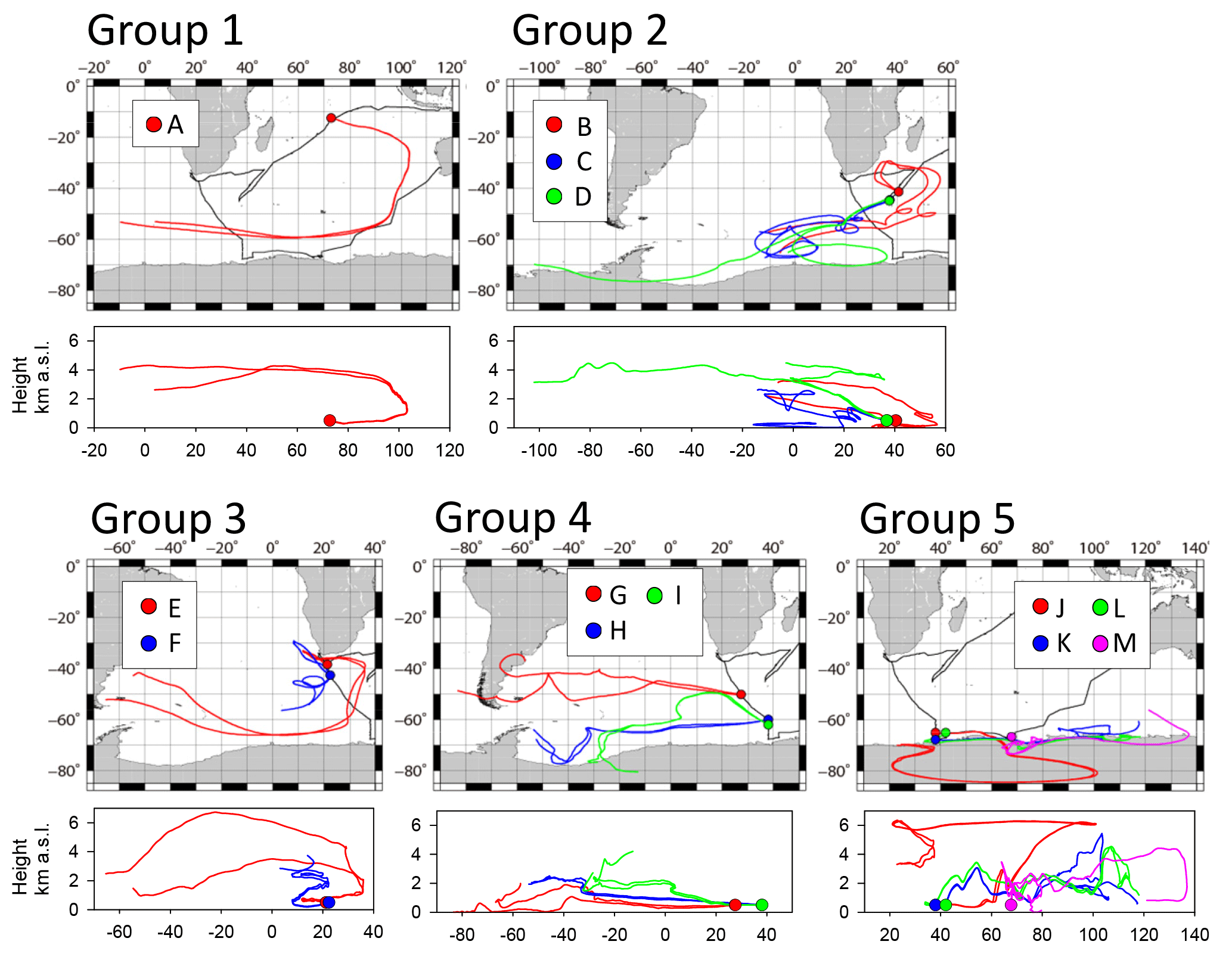
Figure 8TEM sampling location A–M and the 10-day backward trajectories for air masses reaching the location at 500 m a.s.l. during sampling periods. Black lines show the ship track. Colored (red, blue, green, and pink) circles and lines respectively represent sampling locations and backward trajectories.
Table 1TEM samples used for this study and analyzed particle and soot-containing particle numbers.
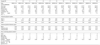
* total data for stages 1 and 2.
Samples were classified into five groups referring to the area. Sample A was collected over the eastern Indian Ocean (classified as group 1). Only one sample was adequate for TEM analysis because of frequent contamination in the eastern Indian Ocean caused by surrounding ship activities. Samples B, C, and D were collected over the western Indian Ocean and were classified as group 2. Samples E and F were collected near southern Africa (classified as group 3). Samples G, H, and I were collected at 50–62∘ S south of South Africa (classified as group 4). Samples J, K, L, and M were collected over the Southern Ocean near the Antarctic coast (classified as group 5).
3.3.2 Morphological features and mixing states
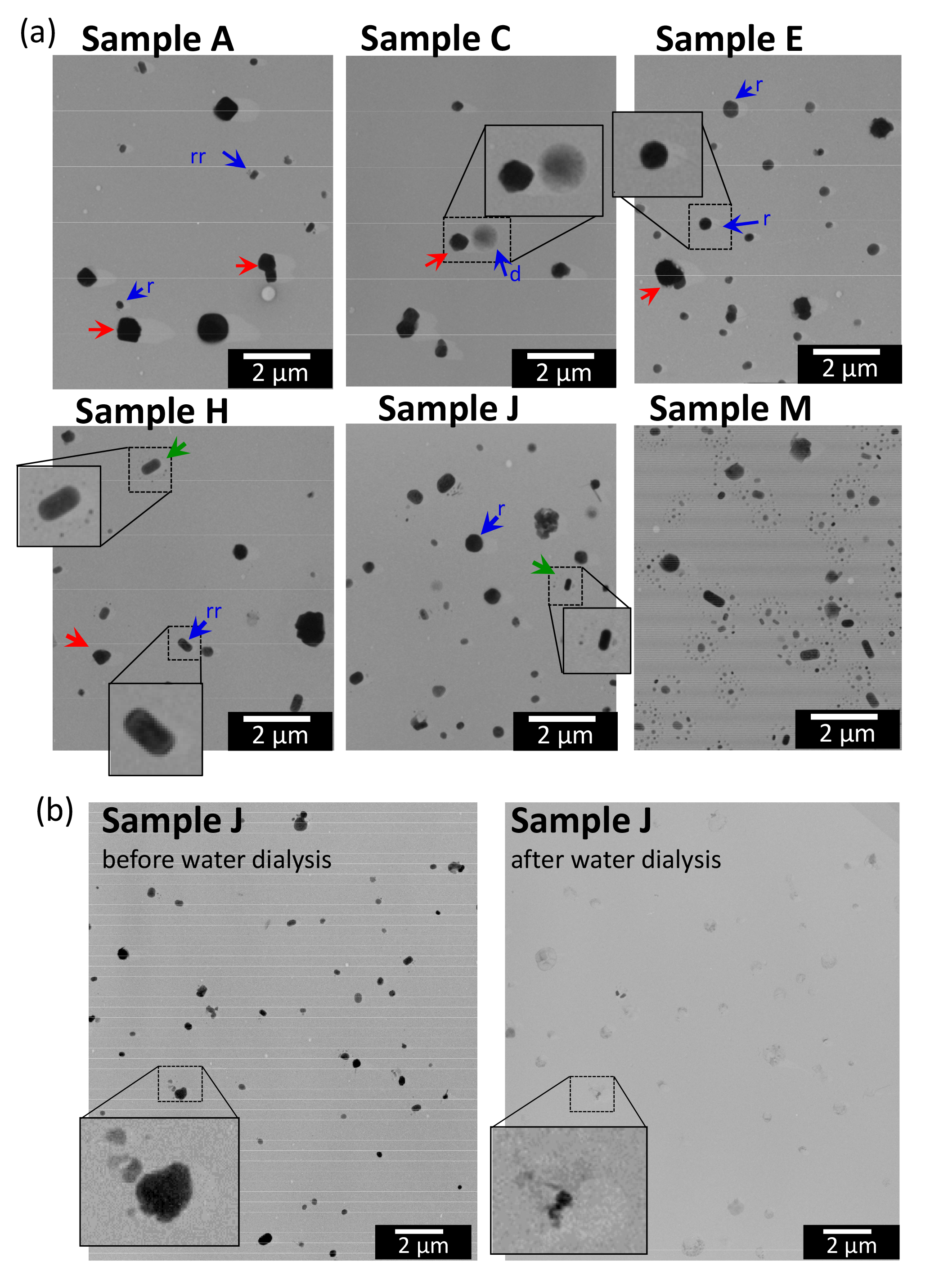
Figure 9Electron micrographs for (a) samples A, C, E, H, J, and M, and (b) before and after dialysis of sample J for the same sample region. Magnifications of all microphotographs of (a) are the same. Red arrows indicate examples of particles with a sea-salt shape. Blue arrows indicate examples of particles with a sulfate particle shape (d, dome-like, r, round, and rr, rotundate rectangular particles). Particles with a satellite structure in samples H and J are marked by green arrows. See main text.
Figure 9 shows TEM images of samples A, C, E, H, J, and M, and an example (lower part) of analysis at the same magnification using water dialysis before and after treatment of sample J. Based on the image contrast and shadow of Pt ∕ Pd of the particle, most of the particles were classified as round (r), dome-like (d), or rotundate rectangular (rr) on the film (examples indicated by blue arrows in Fig. 9a). According to earlier studies based on elemental analysis using an energy-dispersive X-ray spectrometer, such particles were often recognized as sulfate-rich particles (Li et al., 2003; Li and Shao, 2010; Ueda et al., 2011b, 2014, 2016b). Particularly, rotundate rectangular particles were identified as ammonium sulfate particles based on selected-area electron diffraction analysis (Ueda et al., 2011b). Some crystalline coarse particles were also found in group 1–4 samples (samples A–I) (examples are indicated by red arrows in Fig. 9a). These particles showed a stronger contrast with the collection film and had larger diameters than those of sulfate-like particles. Most of them had a cuboidal shape, which is a morphological feature of sea-salt particles. By contrast, such sea-salt-like particles were rarely found in samples (samples J–M) of group 5 collected under lower wind speed conditions near the coast of Antarctica. In samples K, L, and M, most particles exhibited a satellite structure, resembling those of sample M of Fig. 9a. Such particles with a satellite structure were also found in samples H–J collected over the Southern Ocean, as indicated by green arrows. The satellite structure is typically formed by the impact of sulfuric acid (H2SO4) droplets (Waller et al., 1963; Frank and Lodge, 1967; Gras and Ayers, 1979). Some reports have indicated that the satellite ring shape was correlated with the degree of ammonization: a single ring for bisulfate (NH4HSO4) and multiple rings for pure sulfuric acid (Bigg, 1980; Ferek et al., 1983; Ueda et al., 2011b). In this study, some rectangular particles showed a satellite structure, which suggests impact by sulfuric acid droplets. Rectangular particles are usually regarded to be fully neutralized ammonium sulfate. Therefore, the existence of such particles invites curiosity. One possibility for the origin is the transformation of acidic particles after collection by neutralization with ambient ammonia over the substrate. In samples K, L, and M, which were collected closer to the coast of Antarctica, most particles showed a satellite structure with multiple rings, although the satellite particles were fewer in samples H, I, and J than in samples K–M.
As shown in Fig. 9b, water-dialysis analysis reveals that most aerosol particles (i.e., rounded, dome-like rectangular and crystalline-coarse particles, and the satellite particles) were water-soluble. However, quite rarely, insoluble residuals remained after water dialysis. Some of them revealed aggregations of globules with a diameter less than 50 nm, which is characteristic of soot particles (Janzen, 1980; Pósfai et al., 2004; Murr and Soto, 2005). In this study, particles containing such water-insoluble aggregated residuals were regarded as soot-containing particles. Using this method, insoluble materials of less than 0.1 µm diameter were not identifiable as soot because of TEM image quality.
The number of soot-containing particles was 1–10 per sample (Table 1). The number fractions of soot-containing particles to total particles for all samples except for sample H were 1 % or less. The fraction for sample H was 2 %. Although the trajectory did not pass over subtropical areas of South America (Fig. 8), the sampling site of sample H coincided with higher nss-K+ concentrations and higher babs, suggesting some influence from biomass burning.
Several examinations of moderately remote atmospheres using the same water-dialysis analysis have also reported the number fraction of soot-containing particles (Hasegawa and Ohta, 2002; Ueda et al., 2011b). The quantities of soot-containing particles in this study (less than 2 %) were smaller than their values (3–11 % for particles 0.08–1.6 µm at Fukue Island in northwestern Japan by Hasegawa and Ohta, 2002, and 2–25 % for particles 0.2–0.4 µm and 14–59 % for particles 0.4–0.7 µm at Cape Hedo in southwestern Japan by Ueda et al., 2011b). For the soot-containing fraction in the remote marine troposphere above the Southern Ocean, Pósfai et al. (1999) reported that 10–45 % for particles > 0.1 µm were sulfate particles containing soot inclusions based on TEM analysis. They also identified aircraft emissions and biomass burning as the most likely major sources of soot. By contrast, our study examined aerosols within the marine boundary layer by ship. Most sampling sites were more distant from continental source areas than those explained in earlier studies. In addition, the backward air mass trajectories had not passed over continental areas (except Antarctica) for a week. The low fraction of soot-containing particles in this study is expected to be a result of remoteness of the atmosphere observed.
3.3.3 Features of soot-containing particles
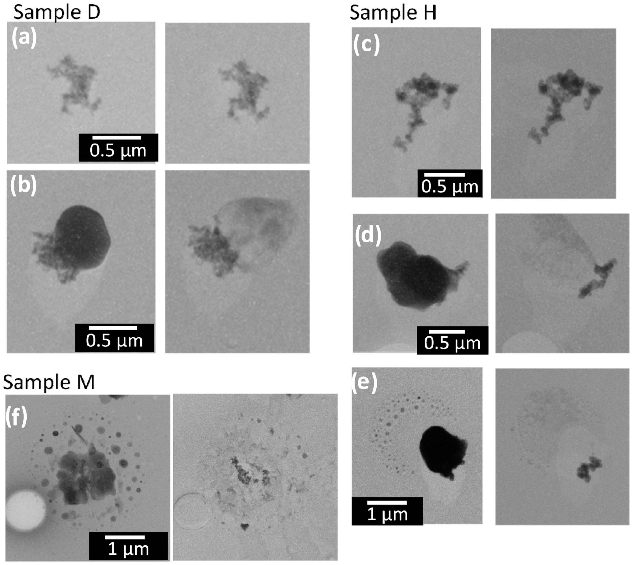
Figure 10Electron micrographs of soot-containing particles before (left) and after (right) water dialysis at the same magnification for samples D, H, and M.
Figure 10 presents representative examples of electron micrographs of soot-containing particles before and after water dialysis at the same magnification. In sample D collected over the western Indian Ocean, soot-containing particles of two types were found: bare soot (i.e., external mixture of soot) and internal mixtures of soot and water-soluble materials. Soot-containing particles of both types were also found in sample H. Some particles that were internally mixed with soot had the satellite structure in sample H, suggesting the existence of acidic droplets. In sample M, all soot was internally mixed with the satellite particles.
Table 2 presents the number and a percentage of each type of soot-containing particle and average values of parameters of soot-containing particles (diameters of soot-containing original particles and inner soot core, and diameter ratios of soot to original particle) for each group. The data are total figures for stages 1 and 2. Figure 11 portrays scatterplots of particle sizes (projected area diameters) before (soot-containing particles: Dparticle) and after (soot: Dsoot) water dialysis of soot-containing particles for groups 1–5. Most Dsoot particles were of 0.1–0.5 µm diameter (Fig. 11). Although some soot-containing particles were of super-micrometer size, Dparticle were mostly submicrometer size.
Table 2Parameters of the soot-containing particles of TEM samples.
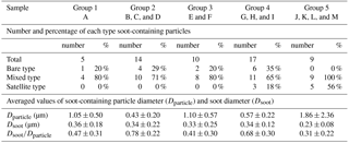
The numbers after the ± symbol denote standard deviation.
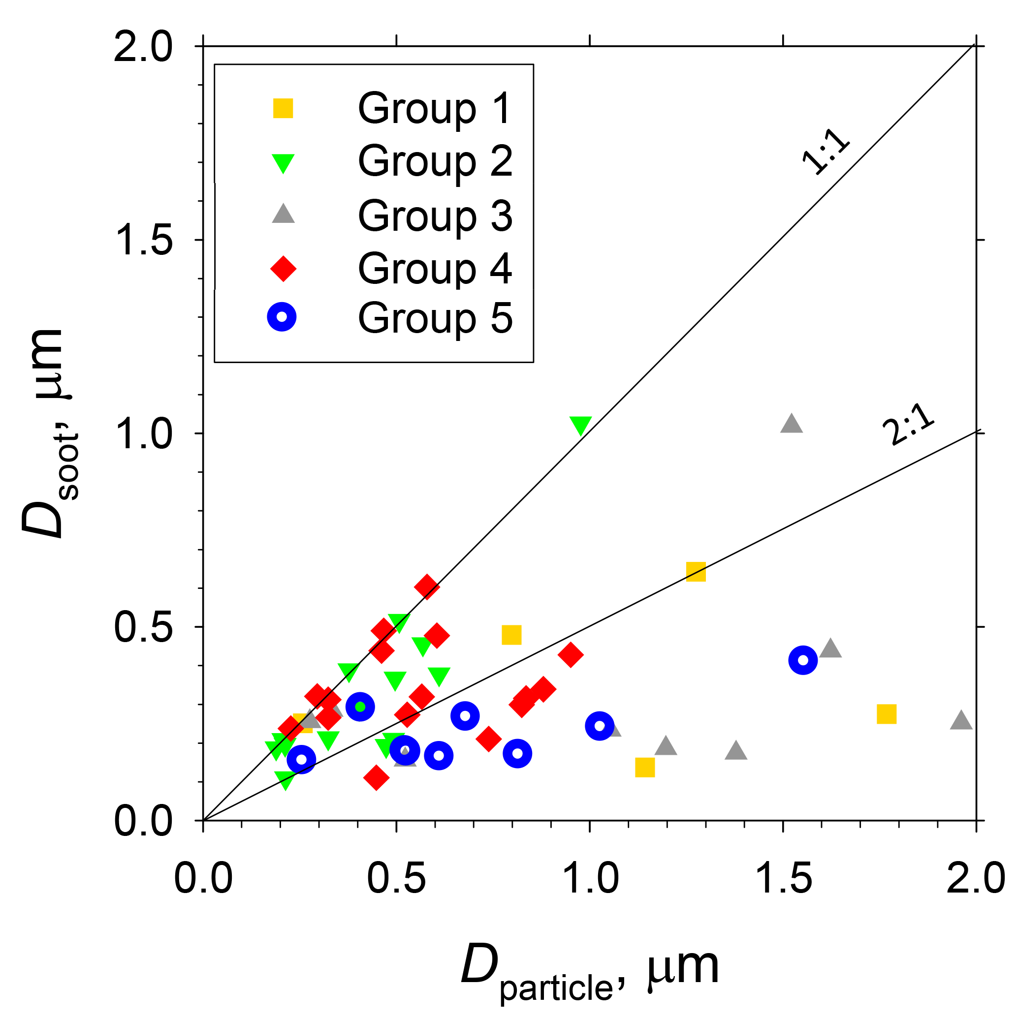
Figure 11Scatterplot of particle sizes before and after water dialysis of soot-containing particles (i.e. soot-containing particle diameter and soot diameter) for sample groups 1–5.
In samples of groups 1–4, 20–35 % of soot-containing particles were found to be bare soot (Table 2). More than half of soot-containing particles of groups 1–4 had diameters of Dparticle less than twice those of Dsoot (Fig. 11). Averaged values of the ratio of Dsoot to Dparticle were 0.41–0.78 (Table 2). Averaged values of Dparticle were largest for group 5 (Table 2). This result disagreed with the high babs ratios of 0.5 to 1.0 µm near Antarctica, as explained in Sect. 3.1. A comparison between results of PSAP and morphological data presented some difficulties. The number and volume of soot particles were quite low in remote ocean areas, especially in the Southern Ocean, compared to the other aerosol materials. Therefore, the possibility that babs of each size range was overestimated by scattering particles was undeniable. In addition, accurate estimation of the diameters of the satellite and liquid particles was difficult. For that reason, the size is expected to differ from the aerodynamic size used in measurement of babs. This section presents discussion of the morphological features of soot-containing particles.
Soot particles that had been freshly emitted from fossil fuel combustion were found to be of bare type (Weingartner et al., 1997). However, aged soot particles often showed coatings of large amounts of secondarily formed materials (Pósfai et al., 1999; Hasegawa et al., 2002; Ueda et al., 2011, 2016b; Adachi et al., 2014). In this study, the air masses for groups 1–4 remained over remote ocean areas without passing continental areas within 8 days (Fig. 8). Nevertheless, a certain number of bare soot particles and less coated soot particles were found in these samples. We have considered that such bare soot might have originated from distant ships (e.g., cargo ships) in the same region or an upper tropospheric source from aircraft emissions. However, the locations of our TEM sample collection for groups 2 and 4 were far from a major ship route located from north of the Malacca Strait to south of Madagascar (Tournadre, 2014). For groups 2 and 4, although the backward trajectory passed a major ship route a few days before for sample B and 10 days before for sample G, that for the other samples did not. Therefore, contributions from distant ships cruising along the major traffic route on days near the sampling days are regarded to be quite low for groups 2 and 4 except sample B. Similarly, the possibility of a contribution from aircraft exhaust is quite low. Most of the backward trajectories for samples of groups 1–4 were passed below 2 km a.s.l. during the 5 days preceding sample collection. In addition, most of the horizontal backward trajectories did not pass through major routes of civil aviation (Stettler et al., 2013) for several days before sampling.
Internally mixed soot particles with soluble materials can be scavenged preferentially from the atmosphere by cloud and rain processes. This mechanism can also engender a higher likelihood of smaller and hydrophobic soot particles surviving longer in the atmosphere. Studies of partitioning of soot particles between cloud droplets and cloud interstitial particles at high altitudes have demonstrated that soot particles remained in interstitial particles and that sulfate particles were more likely to be scavenged to cloud droplets (Hallberg et al., 1992, 1994; Kasper-Giebl et al., 2000; Hitzenberger et al., 2001). Additionally, individual particle analysis using water dialysis revealed that bare soot particles are abundant in cloud interstitial particles under high precipitation (2–6 mm h−1) at a high-elevation mountain site (Ueda et al., 2011a). Wet processes can also scavenge precursor gases for aging particles. Therefore, aging of soot particles will occur slowly in a clean air mass over remote ocean areas. Particularly, weather around 50∘ S was often rainy and stormy during the cruise. During this study, fog and rain events were observed frequently near sampling sites G2 (Fig. 4) and G4 (Fig. 5). Therefore, bare soot particles found in these samples might have come through these wet scavenging processes after they were emitted at a remote source from the sampling site.
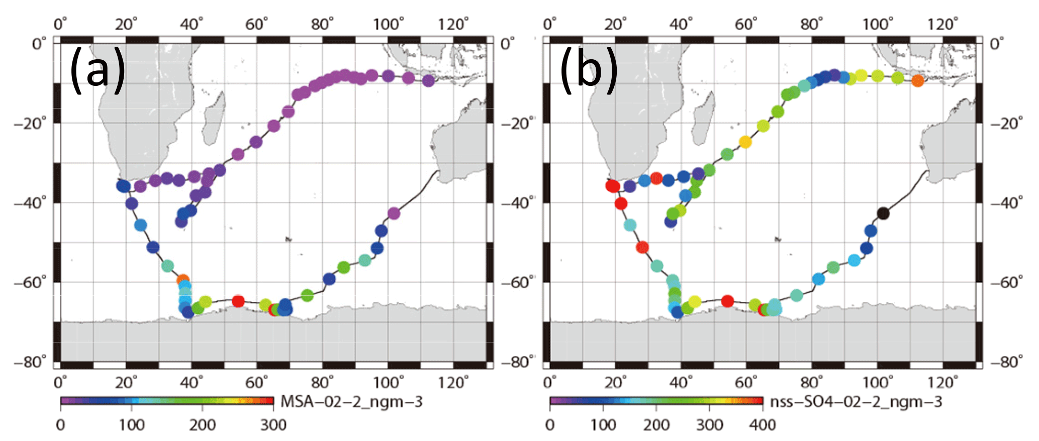
Figure 12Horizontal variation of mass concentrations of (a) for 0.2–2 µm aerosols and (b) nss- for 0.2–2 µm aerosols.
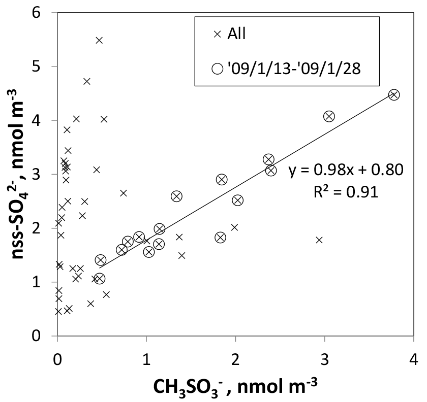
Figure 13Scatterplot of and nss- for 0.2–2 µm aerosols. Crosses and circled crosses respectively represent data for all samples and for samples collected at sites of latitudes higher than 60∘ S (from to ). The fitting line is linearized for circled crosses.
Although some bare soot particles were present over the remote Indian Ocean and northern parts of the Southern Ocean, all soot-containing particles in samples of group 5 collected near the Antarctic coast were mixed internally with water-soluble materials. The values of Dsoot were less than 0.5 µm (Fig. 11). However, most soot-containing particles had Dparticle greater than twice the value of Dsoot. The average ratios of Dsoot to Dparticle were 0.31 (Table 2). The abundance of soot-containing particles with a satellite structure was 56 % in group 5. Such soot-containing particles with a satellite structure were found only in samples obtained at south of 60∘ S latitude. Figure 11a and b respectively portray horizontal distributions of and nss- concentrations for 0.2–2 µm particles. Although nss- has both natural and anthropogenic sources, in marine aerosols is derived from the oxidation of dimethyl sulfide (DMS) emitted by marine phytoplankton (Savoie et al., 1992). Actually, the concentrations in Fig. 12 were higher south of 50∘ S and were quite low at lower (< 30∘ S) latitudes. Sporadic high concentrations of (> 150 ng m−3) were found in coastal areas of Antarctica. High nss- concentrations over the Southern Ocean correspond well with the high concentration for . Figure 13 presents a scatterplot of concentrations of and nss-. For the Southern Ocean of latitudes higher than 60∘ S, nss- concentration showed good correlation with . In addition, the number–size distribution of submicrometer aerosols over the Southern Ocean was characterized by abundant smaller particles (Fig. 5a). These results suggest strongly that submicrometer aerosols over the Southern Ocean are dominated by secondary particles produced by DMS oxidation after local marine biogenic emission. Because DMS production and oxidation are both high in summer in the Southern Ocean, condensation of oxidation products by gaseous DMS and coagulation of the ultrafine particles engender transformation of soot particles and the formation of soot-containing particles coated by sulfuric acid or methanesulfonic acid droplets. Such mixing processes of soot should be considered during the estimation of transport and deposition of BC to Antarctica.
To elucidate the mixing states and morphological features of soot-containing particles in remote marine areas, we conducted shipborne aerosol observations over the Southern and southern Indian oceans during the 27th Umitaka-maru cruise. After TEM samples for individual particle analysis using water dialysis were obtained, 13 samples were chosen for detailed analysis by sampling location and babs.
Water-dialysis examination revealed that many particles in the 13 TEM samples contained water-soluble materials. Regarding the particle number fraction, 0.03–2.11 % of particles on the samples contained chain-like insoluble residuals (soot) of 0.1–0.5 µm diameter.
For samples collected over the southern Indian Ocean and northern Southern Ocean, north of 62∘ S latitude, 20–35 % of soot-containing particles were found to be bare soot. The backward air mass trajectories suggested that most of the sample air had not been affected by aircraft and ship emissions within several days at least. The origin of bare soot remains unknown. Preferential scavenging of aged soot-containing particles might be a mechanism supporting the existence of bare soot over remote ocean areas. On the other hand, all soot-containing particles in samples collected near the Antarctic coast were mixed internally with water-soluble materials. The ratio of diameter of soot ∕ soot-containing particles for samples obtained near the Antarctic coast (0.31) was smaller than those of the other samples (0.41–0.78), suggesting thicker coating than in other places. Most (56 %) of the soot-containing particles near the Antarctic coast had a satellite structure formed by the impact of droplets such as sulfuric acid. Chemical analysis of submicrometer particles near the Antarctic coast revealed high concentrations of non-sea-salt (nss) and of .
This study specifically addressed individual features of soot-containing particles in a remote maritime boundary layer, which was distant from the emission sources of soot. Morphological features of soot-containing particles over the Southern Ocean suggest that aged soot-containing particles were transformed by soluble materials derived from DMS oxidation. Differences of mixing states and transformation of soot-containing particles for various ocean areas must be considered for the evaluation of long-range transport of soot particles and for the simulation of the proper climatic effects of soot-containing particles in the atmosphere.
The back-trajectory data were calculated from the NOAA HYSPLIT model (http://ready.arl.noaa.gov/HYSPLIT.php, last access: 16 May 2016). The other data are available from the corresponding authors upon request.
The authors declare that they have no conflict of interest.
We are indebted to staff members of the Umitaka Maru for assisting our work
on board. We wish to express gratitude to Toshiaki Goto at the Technical
Center of Nagoya University for technical advice on electron microscopy. We
gratefully acknowledge the NOAA Air Resources Laboratory (ARL) for providing
the HYSPLIT transport model (http://ready.arl.noaa.gov/HYSPLIT.php, last acccess: 16 May 2016). This work
was conducted with the support of a grant-in-aid for Environmental Research
provided by the Steel Foundation for Environmental Protection Technology,
and the support of a grant-in-aid for Scientific Research in Priority Areas,
grant no. 18067005 (W-PASS), provided by the Ministry of Education, Culture,
Sports, Science, and Technology, Japan, and by grants-in-aid for Scientific
Research (B) 20310009 and 15H02803, and (A) 20244078 from the Ministry of
Education, Culture, Sports, Science, and Technology. This research is a
contribution of IGBP/SOLAS activity.
Edited by: Allan Bertram
Reviewed by: two anonymous referees
Adachi, K., Zaizen, Y., Kajino, M., and Igarashi, Y.: Mixing state of regionally transported soot particles and the coating effect on their size and shape at a mountain site in Japan, J. Geophys. Res.-Atmos., 119, 5386–5396, https://doi.org/10.1002/2013JD020880, 2014.
Andreae, M. O.: Soot carbon and excess fine potassium: long-range transport of combustion-derived aerosols, Science, 220, 11481151, https://doi.org/10.1126/science.220.4602.1148, 1983.
Bigg, E. K.: Comparison of aerosol at four baseline atmospheric monitoring stations, J. Appl. Meteorol., 19, 521–533, https://doi.org/10.1175/1520-0450(1980)019<0521:COAAFB>2.0.CO;2., 1980.
Bond, T. C., Anderson, T. L., and Campbell, D.: Calibration and intercomparison of filter-based measurements of visible light absorption by aerosols, Aerosol Sci. Tech., 30, 582–600, https://doi.org/10.1080/027868299304435, 1999.
Bond, T. C., Doherty, S. J., Fahey, D. W., Forster, P. M., Berntsen, T., DeAngelo, B. J., Flanner, M. G., Ghan, S., Kärcher, B., Koch, D. Kinne, S., Kondo, Y., Quinn, P. K., Sarofim, M. C., Schultz, M. G., Schulz, M., Venkataraman, C., Zhang, H., Zhang, S., Bellouin, N., Guttikunda, S. K., Hopke, P. K., Jacobson, M. Z., Kaiser, J. W., Klimont, Z., Lohmann, U., Schwarz, J. P., Shindell, D., Storelvmo, T., Warren, S. G., and Zender, C. S.:, Bounding the role of black carbon in the climate system: A scientific assessment, J. Geophys. Res.-Atmos., 118, 5380–5552, https://doi.org/10.1002/jgrd.50171, 2013.
Chaubey, J. P., Moorthy, K. K., Babu, S. S., Nair, V. S., and Tiwari, A.: Black carbon aerosols over coastal Antarctica and its scavenging by snow during the Southern Hemispheric summer, J. Geophys. Res., 115, D10210, https://doi.org/10.1029/2009JD013381, 2010.
Chen, Y., Morton, D. C, Jin, Y., Collatz, G. J., Kasibhatla, P. S., Werf, G. R., DeFries, R. S., and Randerson, J. T: Long-term trends and interannual variability of forest, savanna and agricultural fires in South America, Carbon Manag., 4, 617–638, https://doi.org/10.4155/cmt.13.61, 2013.
Croft, B., Lohmann, U., and von Salzen, K.: Black carbon ageing in the Canadian Centre for Climate modelling and analysis atmospheric general circulation model, Atmos. Chem. Phys., 5, 1931–1949, https://doi.org/10.5194/acp-5-1931-2005, 2005.
Edwards, D. P., Emmons, L. K., Gille, J. C., Chu, A., Attié, J.-L, Giglio, L., Wood, S. W., Haywood, J., Deeter, M. N., Massie, S. T., Ziskin, D. C., and Drummond, J. R.: Satellite-observed pollution from Southern Hemisphere biomass burning, J. Geophys. Res., 111, D14, https://doi.org/10.1029/2005JD006655, 2006.
Evangelista, H., Maldonado, J., Godoi, R. H. M., Pereira, E. B., Koch, D., Tanizaki-Fonseca, K., Grieken, R., Sampaio, M., Setzer, A., and Alencar, A.: Sources and transport of urban and biomass burning aerosol black carbon at the South–West Atlantic Coast, J. Atmos. Chem., 56, 225–238, https://doi.org/10.1007/s10874-006-9052-8, 2007.
Ferek, R. J., Lazrus, A. L., and Winchester, J. W.: Electron microscopy of acidic aerosols collected over the northeastern United States, Atmos. Environ., 17, 1545–1561, https://doi.org/10.1016/0004-6981(83)90308-6, 1983.
Fiebig, M., Lunder, C., and Stohl, A.: Tracing biomass burning aerosol from South America to Troll Research Station, Antarctica, Geophys. Res. Lett., 36, 14, https://doi.org/10.1029/2009GL038531, 2009.
Frank, E. R. and Lodge, J. P.: Morphological identification of airborne particles with the electron microscope, J. Microscope, 6, 449–456, 1967.
Gelencsér, A: Carbonaceous aerosol, Atmospheric and Oceanographic Sciences Library, vol. 30, Springer, Netherlands, 350 pp., 2004.
Giglio, L., Csiszar, I., and Justice, C. O.: Global distribution and seasonality of active fires as observed with the Terra and Aqua Moderate Resolution Imaging Spectroradiometer (MODIS) sensors, J. Geophys. Res., 111, G02016, https://doi.org/10.1029/2005JG000142, 2006.
Gras, J. L. and Ayers, G. P.: On sizing impacted sulfuric acid aerosol particles, J. Appl. Meteorol., 18, 634–638, https://doi.org/10.1175/1520-0450(1979)018<0634:OSISAA>2.0.CO;2, 1979.
Hallberg, A., Ogren, J. A., Noone, K. J., Heintzenberg, J., Berner, A., Solly, I., Kruisz, C., Reischl, G., Fuzzi, S., Facchini, M. C., Hansson, H.-C., Wiedensohler, A., and Svenningsson, I. B.: Phase partitioning for different aerosol species in fog, Tellus, 44B, 545–555, https://doi.org/10.1034/j.1600-0889.1992.t01-2-00008.x, 1992.
Hallberg, A., Ogren, J. A., Noone, K. J., Okada, K., Heintzenberg, J., and Svenningsson, I. B.: The influence of aerosol particle composition on cloud droplet formation, J. Atmos. Chem., 19, 153–171, https://doi.org/10.1007/978-94-011-0313-8_8, 1994.
Hansen, A. D. A., Rosen, H., and Novakov, T.: The aethalometer-an instrument for the real time measurement of optical absorption by aerosol particles. Sci. Total Environ. 36, 103–110, 1984.
Hansen, A. D. A., Lowenthal, D. H., Chow, J. C., and Watson, J. G.: Black carbon aerosol at McMurdo Station, Antarctica, Japca J. Air Waste Ma., 51, 593–600, https://doi.org/10.1080/10473289.2001.10464283, 2001.
Hansen, J. and Nazarenko, L., Soot climate forcing via snow and ice albedos, P. Natl. Acad. Sci. USA, 101, 423–428, https://doi.org/10.1073/pnas.2237157100, 2004.
Hara, K., Yamagata, S., Yamanocuhi, T., Sato, K., Herber, A., Iwasaka, Y., Nagatani, M., and Nakada, H.: Mixing states of individual aerosol particles in spring Arctic troposphere during ASTAR 2000 campaign, J. Geophys. Res., 108, 4209, https://doi.org/10.1029/2002JD002513, 2003.
Hara, K., Osada, K., kido, M., Hayashi, M., Matsunaga, K., Iwasaka, Y., Yamanouchi, T., Hashida, G., and Fukatsu, T.: Chemistry of sea-salt particles and inorganic halogen species in the Antarctic regions: Compositional differences between coastal and inland stations, J. Geophys. Res., 109, D20208, https://doi.org/10.1029/2004JD004713, 2004.
Hara, K., Osada, K., Yabuki, M., Hayashi, M., Yamanouchi, T., Shiobara, M., and Wada, M.: Measurement of black carbon at Syowa station, Antarctica: seasonal variation, transport processes and pathways, Atmos. Chem. Phys. Discuss., 8, 9883–9929, https://doi.org/10.5194/acpd-8-9883-2008, 2008.
Hara, K., Osada, K., Yabuki, M., Hashida, G., Yamanouchi, T., Hayashi, M., Shiobara, M., Nishita, C., and Wada, M.: Haze episodes at Syowa Station, coastal Antarctica: Where did they come from?, J. Geophys. Res., 115, D14205, https://doi.org/10.1029/2009JD012582, 2010.
Hasegawa, S. and Ohta, S.: Some measurements of the mixing state of soot-containing particle at urban and non-urban sites, Atmos. Environ., 36, 3899–3908, https://doi.org/10.1016/S1352-2310(02)00343-6, 2002.
Haywood, J. M. and Boucher, O.: Estimate of the direct and indirect radiative forcing due to tropospheric aerosols: A review, Rev. Geophys., 38, 513–543, https://doi.org/10.1029/1999RG000078, 2000.
Hitzenberger, R., Berner, A., Giebl, H., Drobesch, K., Kasper-Giebl, A., Loeflund, M., Urban, H., and Puxbaum, H.: Black carbon (BC) in alpine aerosols and cloud water concentrations and scavenging efficiencies, Atmos. Environ., 35, 5135–5141, https://doi.org/10.1016/S1352-2310(01)00312-0, 2001.
Janzen, J.: Extinction of light by highly nonspherical strongly absorbing colloidal particles: spectrophotometric determination of volume distributions for carbon blacks, Appl. Optics, 19, 2977–2985, https://doi.org/10.1364/AO.19.002977, 1980.
Kasper-Giebl, A., Koch, A., Hitzenberger, R., and Puxbaum, H.: Scavenging efficiency of “aerosol carbon” and sulfate in supercooled clouds at Mt. Sonnblick (3106 m a.s.l., Austria), J. Atmos. Chem., 35, 33–46, https://doi.org/10.1023/A:1006250508562, 2000.
Kawakami, N., Osada, K., Nishita, C., Yabuki, M., Kobayashi, H., Hara, K., and Shiobara, M.: Factor controlling sea salt modification and dry deposition of nonsea-salt components to the ocean, J. Geophys. Res., 113, D14, https://doi.org/10.1029/2007JD009410, 2008.
Kawamura, K. and Kaplan, I. R.: Motor exhaust emissions as a primary source for diocarboxylic acids in Los Angeles ambient air, Environ. Sci. Technol., 21, 105–110, https://doi.org/10.1021/es00155a014, 1987.
Koch, D.: Transport and direct radiative forcing of carbonaceous and sulfate aerosols in the GISS GCM, J. Geophys. Res., 106, 20311–20332, https://doi.org/10.1029/2001JD900038, 2001.
Koch, D. and Hansen, J.: Distant origins of Arctic black carbon: A Goddard Institute for Space Studies Model E experiment, J. Geophys. Res., 110, D04204, https://doi.org/10.1029/2004JD005296, 2005.
Koch, D., Schulz, M., Kinne, S., McNaughton, C., Spackman, J. R., Balkanski, Y., Bauer, S., Berntsen, T., Bond, T. C., Boucher, O., Chin, M., Clarke, A., De Luca, N., Dentener, F., Diehl, T., Dubovik, O., Easter, R., Fahey, D. W., Feichter, J., Fillmore, D., Freitag, S., Ghan, S., Ginoux, P., Gong, S., Horowitz, L., Iversen, T., Kirkevåg, A., Klimont, Z., Kondo, Y., Krol, M., Liu, X., Miller, R., Montanaro, V., Moteki, N., Myhre, G., Penner, J. E., Perlwitz, J., Pitari, G., Reddy, S., Sahu, L., Sakamoto, H., Schuster, G., Schwarz, J. P., Seland, Ø., Stier, P., Takegawa, N., Takemura, T., Textor, C., van Aardenne, J. A., and Zhao, Y.: Evaluation of black carbon estimations in global aerosol models, Atmos. Chem. Phys., 9, 9001–9026, https://doi.org/10.5194/acp-9-9001-2009, 2009.
Lewis, E. R. and Schwartz, S. E.: Sea salt aerosol production: Mechanisms, methods, measurement and model-A critical review, Geophys. Monogr., 152, 413 pp., AGU, Washington, D. C., 2004.
Li, W. and Shao, L.: Mixing and water-soluble characteristics of particulate organic compounds in individual urban aerosol particles, J. Geophys. Res., 115, D02301, https://doi.org/10.1029/2009JD012575, 2010.
Li, J., Pósfai, M., Hobbs, P. V., and Buseck, P. R.: Individual aerosol particles from biomass burning in southern Africa: 2, Compositions and aging of inorganic particles, J. Geophys. Res., 108, 8484, https://doi.org/10.1029/2002JD002310, 2003.
Moorthy, K., Satheesh, S., Babu, S., and Saha, A.: Large latitudinal gradients and temporal heterogeneity in aerosol black carbon and its mass mixing ratio over southern and northern oceans observed during a trans-continental cruise experiment, Geophys. Res. Lett., 32, 14, https://doi.org/10.1029/2005GL023267, 2005.
Mossop, S. C.: Stratospheric particles at 20 km, Nature, 199, 325–326, https://doi.org/10.1016/0016-7037(65)90017-7, 1963.
Murr, L. E. and Soto, K. F.: A TEM study of soot, carbon nanotubes, and related fullerene nanopolyhedra in common fuel-gas combustion sources, Mater. Charact., 55, 50–65, 2005.
Narukawa, M., Kawamura, K., Takeuchi, N., and Nakajima, T.: Distribution of dicarboxylic acids and carbon isotopic compositions in aerosols from 1997 Indonesian forest fires, Geophys. Res. Lett., 26, 3101–3104, https://doi.org/10.1029/1999GL010810, 1999.
Okada, K.: Nature of individual hygroscopic particles in the urban atmosphere, J. Meteorol. Soc. Jpn., 61, 727–735, 1983.
Okada, K. and Hitzenberger, R. M.: Mixing properties of individual submicrometer aerosol particles in Vienna, Atmos. Environ., 35, 5617–5628, https://doi.org/10.1016/S1352-2310(01)00126-1, 2001.
Pósfai, M., Anderson, J. R., and Buseck, P. R.: Soot and sulfate aerosol particles in the remote marine troposphere, J. Geophys. Res., 104, D17, 685–693, https://doi.org/10.1029/1999JD900208, 1999.
Pósfai, M., Gelencser, A., Simonics, R., Arato, K., Li, J., Hobbs, P. V., and Buseck, P. R.: Atmospheric tar balls: Particles from biomass and biofuel burning, J. Geophys. Res., 109, D06213, https://doi.org/10.1029/2003JD004169, 2004.
Ramanathan, V. and Carmichael, G.: Global and regional climate changes due to black carbon, Nat. Geosci., 1, 221–227, https://doi.org/10.1038/ngeo156, 2008.
Rolph, G., Stein, A., and Stunder, B.: Real-time Environmental Applications and Display sYstem: READY, Environ. Modell. Softw., 95, 210–228, https://doi.org/10.1016/j.envsoft.2017.06.025, 2017.
Savoie, D. L., Prospero, J. M., Larsen, R. J., and Saltzman, E. S.: Nitrogen and Sulfur Species in Aerosols at Mawson, Antarctica, and their relationship to natural radionuclides, J. Atmos. Chem., 14, 181–204, https://doi.org/10.1007/BF00115233, 1992.
Schwarz, J. P., Spackman, J. R., Gao, R. S., Watts, L. A., Stier, P., Schulz, M., Davis, S. M., Wofsy, S. C., and Fahey, D. W.: Global-scale black carbon profiles observed in the remote atmosphere and compared to models, Geophys. Res. Lett., 37, L18812, https://doi.org/10.1029/2010GL044372, 2010.
Schwarz, J. P., Samset, B. H., Perring, A. E., Spackman, J. R., Gao, R. S., Stier, P., Schulz, M., Moore, F. L., Ray, E. A., and Fahey, D. W.: Global-scale seasonally resolved black carbon vertical profiles over the Pacific, Geophys. Res. Lett., 40, 5542–5547, https://doi.org/10.1002/2013GL057775, 2013.
Sciare, J., Favez, O., Sarda-Estève, R., Oikonomou, K., Cachier, H., and Kazan, V.: Long-term observations of carbonaceous aerosols in the Austral Ocean atmosphere: Evidence of a biogenic marine organic source, J. Geophys. Res., 114, D15, https://doi.org/10.1029/2009JD011998, 2009.
Stein, A. F., Draxler, R. R., Rolph, G. D., Stunder, B. J. B., Cohen, M. D., and Ngan, F.: NOAA's HYSPLIT atmospheric transport and dispersion modeling system, B. Am. Meteorol. Soc., 96, 2059–2077, https://doi.org/10.1175/BAMS-D-14-00110.1, 2015.
Stettler, M. E. J., Boies, A. M., Petzold, A., and Barrett, S. R. H.: Global civil aviation black carbon emission, Environ. Sci. Technol., 47, 10397–10404, https://doi.org/10.1021/es401356v, 2013.
Stier, P., Seinfeld, J. H., Kinne, S., Feichter, J., and Boucher, O.: Impact of nonabsorbing anthropogenic aerosols on clear-sky atmospheric absorption, J. Geophys. Res., 111, D18201, https://doi.org/10.1029/2006JD007147, 2006.
Tournadre, J.: Anthropogenic pressure on the open ocean: The growth of ship traffic revealed by altimeter data analysis, Geophys. Res. Lett., 41, 7924–7932, https://doi.org/10.1002/2014GL061786, 2014.
Ueda, S., Osada, K., and Okada, K.: Mixing states of cloud interstitial particles between water-soluble and insoluble materials at Mt. Tateyama, Japan: Effect of meteorological conditions, Atmos. Res., 99, 325–336, https://doi.org/10.1016/j.atmosres.2010.10.021, 2011a.
Ueda, S., Osada, K., and Takami, A.: Morphological features of soot-containing particles internally mixed with water-soluble materials in continental outflow observed at Cape Hedo, Okinawa, Japan, J. Geophys. Res., 116, D17, https://doi.org/10.1029/2010JD015565, 2011b.
Ueda, S., Hirose, Y., Miura, K., and Okochi, H.: Individual aerosol particles in and below clouds along a Mt. Fuji slope: Modification of sea-salt-containing particles by in-cloud processing, Atmos. Res., 137, D17207, https://doi.org/10.1016/j.atmosres.2010.10.021, 2014.
Ueda, S., Miura, K., Kawata, R., Furutani, H., Uematsu, M., Omori, Y., and Tanimoto, H.: Number–size distribution of aerosol particles and new particle formation events in tropical and subtropical Pacific Oceans, Atmos. Environ., 142, 324–339, https://doi.org/10.1016/j.atmosenv.2016.07.055, 2016a.
Ueda, S., Nakayama, T., Taketani, F., Adachi, K., Matsuki, A., Iwamoto, Y., Sadanaga, Y., and Matsumi, Y.: Light absorption and morphological properties of soot-containing aerosols observed at an East Asian outflow site, Noto Peninsula, Japan, Atmos. Chem. Phys., 16, 2525–2541, https://doi.org/10.5194/acp-16-2525-2016, 2016b.
Vester, B. P., Ebert, M., Barnert, E. B., Schneider, J., Kandler, K., Schütz, L., and Weinbruch, S.: Composition and mixing state of the urban background aerosol in the Rhein-Main area (Germany), Atmos. Environ., 41, 6102–6115, https://doi.org/10.1016/j.atmosenv.2007.04.021, 2007.
Waller, R. E., Brooks, A. G. F., and Cartwright, J.: An electron microscope study of particles in town air, J. Air Wet. Pollut., 7, 779–785, 1963.
Weingartner, E., Burtscher, H., and Baltensperger, U.: Hygroscopic properties of carbon and diesel soot particles, Atmos. Environ., 31, 2311–2327, https://doi.org/10.1016/S1352-2310(97)00023-X, 1997.
Weller, R., Minikin, A., Petzold, A., Wagenbach, D., and König-Langlo, G.: Characterization of long-term and seasonal variations of black carbon (BC) concentrations at Neumayer, Antarctica, Atmos. Chem. Phys., 13, 1579–1590, https://doi.org/10.5194/acp-13-1579-2013, 2013.
Wolff, E. and Cachier, H.: Concentrations and seasonal cycle of black carbon in aerosol at a coastal Antarctic station, J. Geophys. Res., 103, D9, https://doi.org/10.1029/97JD01363, 1998.
Zuberi, B., Johnson, K. S., Aleks, G. K., Molina, L. T., and Molina, M. J.: Hydrophilic properties of aged soot, Geophys. Res. Lett., 32, L01807, https://doi.org/10.1029/2004GL021496, 2005.