Radiative impact of an extreme Arctic biomass-burning event

The aim of the presented study was to investigate the impact on the radiation budget of a biomass-burning plume, transported from Alaska to the High Arctic region of Ny-Ålesund, Svalbard, in early July 2015. Since the mean aerosol optical depth increased by the factor of 10 above the average summer background values, this large aerosol load event is considered particularly exceptional in the last 25 years. In situ data with hygroscopic growth equations, as well as remote sensing measurements as inputs to radiative transfer models, were used, in order to estimate biases associated with (i) hygroscopicity, (ii) variability of single-scattering albedo profiles, and (iii) plane-parallel closure of the modelled atmosphere. A chemical weather model with satellite-derived biomass-burning emissions was applied to interpret the transport and transformation pathways.

The provided MODTRAN radiative transfer model (RTM) simulations for the smoke event (14:00 9 July–11:30 11 July) resulted in a mean aerosol direct radiative forcing at the levels of −78.9 and −47.0 W m⁻² at the surface and at the top of the atmosphere, respectively, for the mean value of aerosol optical depth equal to 0.64 at 550 nm. This corresponded to the average clear-sky direct radiative forcing of −43.3 W m⁻², estimated by radiometer and model simulations at the surface. Ultimately, uncertainty associated with the plane-parallel atmosphere approximation altered results by about 2 W m⁻². Furthermore, model-derived aerosol direct radiative forcing efficiency reached on average −126 W m${}^{-\mathrm{2}}/{\mathit{\tau }}_{\mathrm{550}}$ and −71 W m${}^{-\mathrm{2}}/{\mathit{\tau }}_{\mathrm{550}}$ at the surface and at the top of the atmosphere, respectively. The heating rate, estimated at up to 1.8 K day⁻¹ inside the biomass-burning plume, implied vertical mixing with turbulent kinetic energy of 0.3 m² s⁻².

1 Introduction

Wildfires are considered significant sources of carbon in the atmosphere. It is estimated that up to 2.0 Pg of carbon aerosol is released into the atmosphere each year (van der Werf et al., 2010) due to wildfires. In the past 100 years, an intensification of fires in the mid-latitudes has been observed to appreciably affect radiative and optical properties of the atmosphere (Mtetwa and McCormick, 2003). Emissions from biomass-burning (BB) sources consist mainly of organic and black carbon particles (IPCC, 2001), of which 90 % are made of the fine mode aerosol size distribution (Dubovik et al., 2002). The impact of the plume on the atmospheric instability conditions and its rather small particle radius property may result in rapid transport on an intercontinental scale within just several days (Nikonovas et al., 2015). The presence of BB aerosol causes heating of the air layer in which the transport takes place. Regarding the columnar properties, however, smoke existence results in a weak cooling at the top of the atmosphere (TOA) due to predominant scattering properties of the plume (Hansen et al., 2004). The magnitude of its impact on the radiative properties is nevertheless strongly dependent on the chemical composition of the smoke plume, due to the adversative radiative responses of the atmosphere exposed to black and organic carbon, being negative for the latter (Myhre et al., 2013a).

A number of papers analysed the annual mean value of instantaneous clear-sky aerosol direct radiative forcing (RF) at the TOA (RF_toa) associated with BB plumes. Myhre et al. (2013a) presented the results from 28 AeroCom Phase II models, indicating a global mean BB RF_toa of approximately −0.01 ± 0.08 W m⁻². A similar value of 0.0 ± 0.2 W m⁻² was presented by Myhre et al. (2013b) in the Fifth Assessment IPCC Report. Despite a rather low (and negative) mean global value of BB RF_toa, on a regional scale (especially over bright surfaces) smoke may well play a substantial role in affecting radiative properties of the atmosphere (Wang et al., 2006). In the case of high surface albedo, the existence of smoke particles leads to the decrease in columnar albedo at the TOA. This may in turn indicate a positive RF_toa (Screen and Simmonds, 2010), leading to positive feedback within the entire atmospheric column. Based on AeroCom Phase II multi-model evaluations, Sand et al. (2017) found the annual median value of ensemble RF_toa in the Arctic region to be 0.01 W m⁻². Similar results are presented in Wang et al. (2014), who estimated its value at around 0.004 W m⁻².

The significantly high RF uncertainty is mainly associated with the approximations of surface properties dependent on the daily and seasonal cycles, as well as the aerosol optical and microphysical properties which undergo ageing processes, whilst being transported across a large region (Bond et al., 2013; Ortiz-Amezcua et al., 2017; Koch et al., 2009; Janicka et al., 2017). The accurate parametrization of aerosol single-scattering properties as inputs to radiative transfer simulations at a regional scale is of great concern in the Arctic region, due to sparse spatial distribution of long-term ground-based measurements (Markowicz et al., 2017a) and a high mean cloud fraction (especially in the summer), which limits satellite retrievals. In single-cell simulations at a certain location, aerosol single-scattering properties might be investigated by inversion schemes using sun-photometer data retrieved under AERONET (AErosol RObotic NETwork; Holben et al., 2001). However, the uncertainty in the columnar single-scattering albedo (ω) retrieval becomes high, considering low levels of aerosol optical depth (τ; Dubovik et al., 2000). This is the reason why AERONET level 2 data validation is performed only for τ₄₄₀ larger than 0.5 and solar zenith angles above 50^∘ (Dubovik et al., 2002). This, in turn, leads to a significant reduction of data coverage calculated for the Arctic region (Markowicz et al., 2017a).

The above aerosol properties may also be calculated using in situ measurements. It should be taken into account that such measurements are usually carried out at around 20–30 ^∘C (at which water evaporation occurs), leading to a reduction of aerosol optical properties associated with their hygroscopic properties. The impact of water uptake by aerosol is significant for soluble particles when exposed to a relative humidity (RH) of more than 40 %, resulting in the enhancement of a particle scattering cross section (Orr et al., 1958). Some studies apply empirical formulas of an enhancement factor f(RH) to retrieve the aerosol optical properties at ambient conditions (Kotchenruther and Hobbs, 1998). The factor is defined as the ratio between particle radius at ambient conditions and RH fixed to 30 %. The absolute values of the enhancement factor may vary significantly due to the particle chemical composition related to the emission source (Gras et al., 1999; Magi et al., 2003; Kreidenweis et al., 2001) and due to particle size (Carrico et al., 2010). Fresh and aged plumes of BB aerosol f(RH) were found to be 1.1 and 1.35, respectively (at a RH of around 80 %). This f(RH) enhancement due to the ageing process is in agreement with the secondary production of sulphate and progressive oxidation of organic compounds with OH and COOH groups, which result in increasing the hygroscopic properties (Reid et al., 2005).

The study of smoke transport over the Arctic during July 2015 has been previously presented in scientific papers and is also characterized in this research. Markowicz et al. (2016a) reported the temporal and spatial variability in aerosol single-scattering properties measured by in situ and ground-based remote sensing instruments over Svalbard and in Andenes, Norway. Moroni et al. (2017), discussed morphochemical characteristics and the mixing state of smoke particles at Ny-Ålesund, as indicated by a DEKATI 12-stage low-volume impactor combined with scanning electron microscopy. Markowicz et al. (2017b), on the other hand, presented a comprehensive description of smoke radiative and optical properties on a regional scale. The paper examined ageing processes of the smoke plume under study, whilst being transported from the source region and across the High Arctic. A simple Fu–Liou RTM, combined with the NAAPS aerosol transport model, was used to determine the spatial distribution of aerosol single-scattering properties and RFs for the period of 5–15 July 2015, in the area to the north of 55^∘ N, where the transport of BB aerosol was observed.

In this paper, we use MODTRAN radiative transfer simulations and aerosol optical properties obtained from in situ and ground-based remote sensing instruments to retrieve clear-sky direct RF over the area close to Ny-Ålesund. The research aims to estimate the biases connected with (i) hygroscopicity, (ii) variability of ω profiles, and (iii) plane-parallel closure of the modelled atmosphere. The main outcome of this research is the implementation of a new methodology to retrieve the profile of ω at ambient conditions, using in situ measurements and lidar profiles (Sect. 3.2). Simulated RFs were compared to results from a simple RTM (Sect. 3.5). Section 3.6 shows an example of RF distribution at the surface, in the vicinity of Ny-Ålesund (Svalbard). Section 3.7 shows the influence of the BB air masses on the development of the turbulence. Additionally, we confirmed the source region of the BB plume. A chemical weather model with satellite-derived biomass-burning emissions was used to interpret the transport and transformation pathways.

2 Methodology

This section gives a brief description of all data and models used in this research. In Sect. 2.1 we will focus on characterization of all models used to track the transport of smoke, as well as to calculate the impact of the BB plume on radiative and dynamical properties of the atmosphere.

2.1 Modelling tools

The MODerate-resolution atmospheric radiance and TRANsmittance model (MODTRAN) version 5.2.1 (Berk et al., 1998) is the radiative transfer model (RTM) used. In this study, simulations are run with 17 defined absorption coefficients for each band in a correlated-k scheme (multiple scattering included; Bernstein et al., 1996); 8-stream discrete ordinate radiative transfer (DISORT) method, with a spectral resolution of 15 cm⁻¹ of the radiation fluxes (Stamnes et al., 1988); and the Henyey–Greenstein scattering phase function approximation (Henyey and Greenstein, 1941). Calculations are performed for the user-defined vertical profiles of thermodynamic variables (measured by radio sounding), including aerosol and trace gas optical properties, provided by the HITRAN 2000 database (Rothman et al., 1998). MODTRAN was run with a time resolution of 20 min from the 9 to 11 July 2015, for the domain set to Ny-Ålesund coordinates. Simulations included cases with and without aerosol load (i.e. “polluted” and “clean”).

The Fu–Liou version 200503 (Fu and Liou, 1992, 1993) RTM uses the δ2∕4 stream solver, applied for 6 short-wave and 12 long-wave spectral bands. The optical properties of the atmosphere are calculated by the correlated-k distribution method, defined for each spectral band (Fu and Liou, 1992). The optical properties of aerosols, as well as thermodynamic properties of the atmosphere, were based on the results provided by the NAAPS (Navy Aerosol Analysis and Prediction System) global aerosol model reanalysis (Lynch et al., 2016). Fu–Liou simulations, previously published in Markowicz et al. (2017b), were conducted to compare the results obtained by the approach used in this study (see Sect. 2.3.4) applied to MODTRAN RTM.

3-D effects of the RF were calculated using 3-D forward Monte Carlo code (Marshak et al., 1995), which uses a maximum cross-section method to compute photon paths in the three-dimensional model of the atmosphere (Marchuk et al., 2013). A number of modifications were made to the original setup of the code, including such phenomena as absorption of photons by atmospheric gases as well as reflection and absorption at the undulating Earth's surface (Rozwadowska and Górecka, 2012, 2017). The model domain covers the area of 51 km (W–E axis) × 68 km (S–N axis) and consists of cells or columns of 200 m × 200 m. A 20 km wide belt surrounds the main domain, in order to reduce the impact of cyclic boundaries on the results in the Monte Carlo modelling. The computations were performed for the whole 91 km × 108 km domain; however, only the results from the main domain were analysed. The Earth's surface was represented by a digital elevation model (DEM) and the technique proposed by Ricchiazzi and Gautier (1998).

Large-eddy simulations (LESs) were performed using the 3-D non-hydrostatic anelastic Eulerian/semi-Lagrangian (EULAG) model (Prusa et al., 2008) to estimate the dynamical response of the atmosphere induced by the BB plume. The EULAG model was set up to solve for the three velocity components u, v, and w in the x-, y-, and z-directions (i.e. W–E, S–N, and vertical directions), as well as the potential temperature (θ). The governing equations are solved in an Eulerian framework without explicit subgrid-scale terms included, i.e. we use the method of implicit LES (ILESs). The non-oscillatory, forward-in-time integration was performed with the Multidimensional Positive definite Advection Transport Algorithm (MPDATA; Smolarkiewicz, 2006). We relied on the ability of the MPDATA to implicitly account for the effect of unresolved turbulence on the resolved flow, through the truncation terms associated with the algorithm. For more details on ILES, see Grinstein et al. (2007). The horizontal grid spacing was set to 200 m and the vertical grid spacing to 50 m. The size of the computational domain was set to 19 km in the horizontal directions and 20 km in the vertical direction. The uppermost 5 km is a sponge layer included to prevent reflection of gravity waves at the top of the domain. The upper boundary of the domain is impermeable with a free slip condition, while the lower boundary is impermeable with a partial slip condition, characterized by a specified drag coefficient of 0.001. The flow is periodic across the lateral boundaries of the domain. The EULAG simulations were based on results from the RTM (10 July 2015 11:30 UTC) and radio sounding data from Ny-Ålesund obtained on 10 July 2015 12:00 UTC.

Table 1 Description of the instruments installed at Ny-Ålesund, used as input data for the atmospheric RTM.

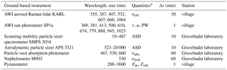
^∗ σ_ext – extinction coefficient, τ – aerosol optical depth, α – Ångstrom exponent, PW – precipitable water, ASD – aerosol size distribution, σ_abs – absorption coefficient, σ_scat – scattering coefficient, F_in – total incoming flux, F_out – total outgoing flux both at the surface.

The Global Environmental Multiscale model with atmospheric chemistry (GEM-AQ; Côté et al., 1998; Kaminski et al., 2008) was run in a global configuration with a uniform grid resolution of 0.9^∘. The vertical domain was defined on 28 hybrid levels with the model top at 10 hPa. BB emissions were taken from the Global Fire Assimilation System (GFAS; Kaiser et al., 2012). In addition to comprehensive tropospheric chemistry, the GEM-AQ model has five size-resolved aerosol species: sea salt, sulphate, black carbon, organic carbon, and dust. The microphysical processes that describe formation and transformation of aerosols are calculated by a sectional aerosol module (Gong, 2003). The particle mass is distributed into 12 logarithmically spaced bins from 0.005 to 10.24 µm. The aerosol module accounts for nucleation, condensation, coagulation, sedimentation and dry deposition, in-cloud oxidation of SO₂, in-cloud scavenging, and below-cloud scavenging by rain and snow. Calculations of τ are done online for all bins and aerosol species. Extinction cross sections are taken from the AODSEM model (Aubé et al., 2000, 2004). Anthropogenic emissions, based on ECLIPSEv4 (http://www.iiasa.ac.at/web/home/research/researchPrograms/air/ECLIPSEv4a.html), were used. The model was run for the period from 15 June to 20 July 2015. Simulations of back-trajectories and chemical composition were used to distinguish the BB layers in the lidar data and to identify the source region of the smoke plume under study.

2.2 Instruments

In this section, we present a brief description of all instruments located at Ny-Ålesund used for this research study (Table 1). For a more detailed specification, please read the section on instrumentation in Markowicz et al. (2016a).

Variables τ, Ångstrom exponent (α), and precipitable water (PW) were measured by a fully automatic sun photometer SP1a (Dr. Schulz & Partner GmbH). The instrument obtains direct solar radiation in 10 channels ranging from 369 and 1023 nm with 1^∘ field of view (Herber et al., 2002). Corrections included temperature variability, Langley methodology, and cloud-screening algorithms (Smirnov et al., 2000; Alexandrov et al., 2004).

Extinction profiles were retrieved from KARL Raman lidar. The instrument uses Nd:Yag laser pulses at 355, 532, 1064 nm with a power of 10 W at each wavelength to obtain backscatter and extinction coefficients. Also, depolarization is measured at water vapour channels (407, 660 nm). The detection is carried out by a 70 cm mirror with a 1.75 mrad field of view, and the overlap issue is fulfilled at 700 m a.g.l. Further details may be found in Hoffmann (2011) and Ritter et al. (2016).

Continuous measurements of radiation fluxes are provided at Ny-Ålesund under the Baseline Surface Radiation Network (BSRN). A ball-shaded CMP22 by Kipp & Zonen installed on a solar tracker by Schulz & Partner measures total incoming and reflected solar radiation at 200–3600 nm (Maturilli et al., 2015).

The in situ measurements of single-scattering properties were provided by the Gruvebadet Laboratory, located 1 km southwest of Ny-Ålesund. The single wavelength M903 nephelometer from Radiance Research, uses a xenon flash lamp and opal diffuser to derive the scattering coefficient at 530 nm (Müller et al., 2009), with an angular integration range of 10–170^∘. Corrections for non-ideal illumination and truncation error were performed according to the description presented in Müller et al. (2009).

Black carbon (BC) concentration and the aerosol absorption coefficient were measured at 467, 530, and 660 nm by the particle soot absorption photometer (PSAP) from Radiance Research, based on the principle of filter attenuation change due to aerosol load. Corrections for multiple scattering and non-purely absorbing aerosols were done following the methodology from Haywood and Osborne (2000).

Aerosol size distribution measurements were covered by joint spectra of the TSI scanning mobility particle sizer (SMPS 3034), with 54 channels, and the TSI aerodynamic particle sizer spectrometer (APS 3321), with 52 channels. Jointly, the spectral coverage is in the range of 10–20 000 nm, excluding a gap around 500 nm which was fitted. Both instruments delivered data with a resolution of 10 min.

2.3 Atmospheric and surface properties – inputs to models

2.3.1 Surface properties

MODIS 6th collection daily product M*D09CMG was used to retrieve surface albedo values over the area between 55 and 90^∘ N with a resolution of 1^∘ × 1^∘. Data were averaged over 1 month to obtain good coverage, assumed constant with time, and inserted into the Fu–Liou model (Markowicz et al., 2017b).

Spectral dependency of surface albedo derived from the MODTRAN built-in module, using calculations of the Fresnel reflection at the ocean top, was applied while comparing data to Fu–Liou results. An additional setup of radiometer-derived surface albedo was used for the comparison with RF, calculated by means of the radiometer measurements. Both MODTRAN and Fu–Liou codes assumed a flat and horizontal Earth surface.

MODIS MCD43A1 surface product of bidirectional reflectance distribution function (BRDF) on 12 July 2015 (closest to the simulation day), at 469 nm, was used for the 3-D Monte Carlo model over the Svalbard area. The BRDF was calculated yielding the equation of Strahler et al. (1999):

$$\begin{array}{ll}{\displaystyle }R(\mathrm{\Theta },\mathit{\vartheta },\mathit{\varphi },\mathit{\lambda })=& {\displaystyle }{f}_{\mathrm{iso}}\left(\mathit{\lambda }\right)+f_{\mathrm{vol}}\left(\mathit{\lambda }\right)\cdot K_{\mathrm{vol}}(\mathrm{\Theta },\mathit{\vartheta },\mathit{\varphi })\\ \text{(1)}& {\displaystyle }& {\displaystyle }+f_{\mathrm{geo}}\left(\mathit{\lambda }\right)\cdot K_{\mathrm{geo}}(\mathrm{\Theta },\mathit{\vartheta },\mathit{\varphi }),\end{array}$$

where f and K stand for coefficient kernels. In particular, “iso” denotes the isotropic scattering component, “geo” the diffuse reflection component, and “vol” the volume scattering component. Variables Θ, ϑ and ϕ are solar zenith angle, view zenith angle and view–sun relative azimuth angle, respectively. The gaps over land were filled in with mean values of parameters for a given surface type (glacier or tundra/rock) and elevation range. The coastal line used to distinguish between water and land was taken from the Norwegian Polar Institute (2014a). Glacier outlines (last updated 1 April 2016) were taken from the Svalbard land covering map data set (Norwegian Polar Institute, 2014b). Fresnel reflection from the water surface was assumed in the modelling. Moreover, radiation scattering by seawater and its constituents (e.g. phytoplankton or mineral suspended matter) was neglected.

The DEM used in the 3-D Monte Carlo modelling was based on maps from the Norwegian Polar Institute (2014a, UTM zone 33N projection, ellipsoid WGS84). The original DEM was regridded to a resolution of 200 m. The land surface altitude within a cell is estimated by the following equation (Ricchiazzi and Gautier, 1998):

$$\begin{array}{}\text{(2)}& z=a_{\mathrm{0}}\cdot x+a_{\mathrm{1}}\cdot y+a_{\mathrm{2}}\cdot x\cdot y+a_{\mathrm{3}},\end{array}$$

where x, y, and z are the coordinates of a given point of a cell surface and a₀, a₁, a₂, and a₃ are coefficients fitted to the coordinates of the cell nodes. The Earth's surface approximated in such a way is continuous.

2.3.2 Vertical profiles of thermodynamic variables and ozone concentration

Profiles of all thermodynamic properties, including pressure (p), temperature, wind speed, and RH, were adopted from the radio soundings performed at Ny-Ålesund for the day of interest. The radio-sounding profiles were complemented by subarctic summer profiles from the international standard atmosphere to extend them up to 100 km. These were further used for the 3-D Monte Carlo, MODTRAN, and EULAG simulations. The profiles for the Fu–Liou calculations were taken from the Navy Operational Global Analysis and Prediction System (NOGAPS).

Vertical profiles of ozone were retrieved from dimensional climatology, UGAMP (Li and Shine, 1995), then scaled to the measured values of the total ozone content by the MODIS M*D09CMG product (Fu–Liou model) and SP1a photometer (the remaining models).

2.3.3 Vertical profiles of aerosol single-scattering properties

Vertical profiles of aerosol single-scattering properties at ambient conditions were used as input parameters to MODTRAN and 3-D Monte Carlo calculations. The retrieval was based on the in situ aerosol single-scattering properties, measured at the surface in dry conditions (denoted hereinafter as superscript “d”), and on vertical profiles of ${\mathit{\sigma }}_{\mathrm{ext}}^{\mathrm{a}}$, as well as RH at ambient conditions (hereinafter superscript “a”) from KARL lidar and radio-sounding data.

In reference to temporal variability in the range-corrected signal measured at 532 nm by the micropulse lidar, Markowicz et al. (2016a) characterize smoke plume as a rather well-mixed layer of BB aerosol extending from around 4–6 km on 9 July to 0–3.5 km later on. Both contributions of BB-like aerosol in the NAAPS τ, estimated on a level as high as 80 %, and the similarity between columnar and in situ aerosol extensive properties, such as α (Markowicz et al., 2016a), suggest that the smoke plume may have crossed the planetary boundary layer, mixing with the lowermost part of the troposphere. Additionally, the infinitesimal aerosol load that exists above the smoke plume plays a minor role in affecting the radiative properties of the atmosphere, and therefore may be neglected. This is why, in the presented methodology, we assume no changes in chemical composition vertically, so that most of the possible vertical variability in ω^a at ambient conditions is attributed to changes in the RH. Therefore, we approximate initial profiles of ω^d and $R_{\mathrm{eff}}^{\mathrm{d}}$ by setting them up to the values of in situ measurements and consider them constant with altitude. By introducing the hygroscopic growth model for particles with known size distribution, one may obtain ω^a profile as well as g^a.

Algorithm for delivering single-scattering albedo ω profile at ambient conditions

From absorption (σ_abs) and scattering (σ_scat) coefficients at 530 nm (for details see Table 1), ω can be calculated, yielding

$$\begin{array}{}\text{(3)}& \mathit{\omega }(\mathit{\lambda },z)=\mathrm{1}-{\displaystyle \frac{{\mathit{\sigma }}_{\mathrm{abs}}(\mathit{\lambda },z)}{{\mathit{\sigma }}_{\mathrm{ext}}(\mathit{\lambda },z)}}\end{array}$$

at ambient and dry conditions. Subsequently, since σ_abs is a weak function of RH (Zieger et al., 2011), the assumption that ${\mathit{\sigma }}_{\mathrm{abs}}^{\mathrm{a}}$ and ${\mathit{\sigma }}_{\mathrm{abs}}^{\mathrm{d}}$ are identical is justified. We can then relate dry and ambient conditions by introducing the scattering enhancement factor f(λ,z(RH)) principle, defined as the ratio between scattering coefficients measured at mentioned RH states (Zieger et al., 2010):

$$\begin{array}{}\text{(4)}& f(\mathit{\lambda },z(\mathrm{RH}\left)\right)={\displaystyle \frac{{\mathit{\sigma }}_{\mathrm{scat}}^{\mathrm{a}}(\mathit{\lambda },z(\mathrm{RH}\left)\right)}{{\mathit{\sigma }}_{\mathrm{scat}}^{\mathrm{d}}(\mathit{\lambda },z)}}.\end{array}$$

Ultimately, from formulas (3) and (4), we may introduce the equation for ω^a satisfying

$$\begin{array}{}\text{(5)}& {\mathit{\omega }}^{\mathrm{a}}(\mathit{\lambda },z)={\displaystyle \frac{\mathrm{1}}{\mathrm{1}+\frac{\mathrm{1}-{\mathit{\omega }}^{\mathrm{d}}(\mathit{\lambda },z)}{{\mathit{\omega }}^{\mathrm{d}}(\mathit{\lambda },z)\cdot f(\mathit{\lambda },z(\mathrm{RH}\left)\right)}}}.\end{array}$$

Therefore, to derive the relationship between the aerosol water uptake and a particular aerosol species, the Hänel model (Hänel, 1976) of growth factor f(RH) is used, relating hygroscopicity of aerosols with relative humidity, yielding

$$\begin{array}{}\text{(6)}& f\left(\mathrm{RH}\right)={\left({\displaystyle \frac{\mathrm{1}-{\mathrm{RH}}^{\mathrm{a}}}{\mathrm{1}-{\mathrm{RH}}^{\mathrm{d}}}}\right)}^{-\mathit{\gamma }},\end{array}$$

where the γ parameter represents the indicator of particle hygroscopicity, a larger γ refers to more hygroscopic aerosols. In this study, a literature value of γ was introduced equal to 0.18, which applies for BB aerosols (Reid et al., 2005). In this method we combine lidar and in situ measurements. The issue of lack of data within the lidar geometrical compression range (0–700 m) is solved by an interpolation method. The proposed method leads to ω^a uncertainty of 0.05, where its vast majority may be attributed to ${\mathit{\sigma }}_{\mathrm{abs}}^{\mathrm{d}}$ and ${\mathit{\sigma }}_{\mathrm{scat}}^{\mathrm{d}}$ measurement uncertainties.

Algorithm for delivering asymmetry parameter g at ambient conditions

Asymmetry parameter g is derived iteratively using aerosol size distributions, measured by SMPS and APS, and Mie theory, as well as a one-parameter equation determined by Petters and Kreidenweis (2007) that approximates the relationship between the RH and the growth factor χ(RH), yielding

$$\begin{array}{}\text{(7)}& \mathit{\chi }\left(\mathrm{RH}\right)={\left(\mathrm{1}+\mathit{\kappa }{\displaystyle \frac{\mathrm{RH}}{\mathrm{1}-\mathrm{RH}}}\right)}^{\frac{\mathrm{1}}{\mathrm{3}}},\end{array}$$

where RH represents the relative humidity, while neglecting the Kelvin effect (in terms of the Köhler law), being true for particles significantly affecting light extinction (diameter > 0.01 µm; Zieger et al., 2011; Bar-Or et al., 2012). Coefficient κ, however, refers to particle hygroscopicity, with respect to the Raoult effect. In this study, for simplification purposes, we neglect the effect of the broadening of the aerosol size distribution spectra, due to diffusional growth of particles. To determine the most accurate literature value of κ coefficient for the BB aerosol, that vastly relies on flora being burnt, we studied the trajectory of smoke transport over the Arctic by means of the GEM-AQ model and analysed a source area in the event under study, i.e. Alaska, regarding vegetation coverage. A κ coefficient of 0.07 (0.25 µm dry diameter) was chosen to match vegetation (Duff core) covering the Alaskan tundra (Carrico et al., 2010).

The size distributions of aerosols at ambient conditions were estimated by introducing the hygroscopic growth factor χ(RH), related to the growth of particles due to water uptake, yielding

$$\begin{array}{}\text{(8)}& \mathit{\chi }\left(\mathrm{RH}\right)={\displaystyle \frac{D^{\mathrm{a}}\left(\mathrm{RH}\right)}{D_{\mathrm{d}}\left(\mathrm{RH}\right)}},\end{array}$$

where D is the diameter of the particle at a certain RH (Zieger et al., 2010).

The calculations are provided for an extreme BB event; thus, as previously mentioned, the concentration of aerosols other than smoke is negligible. That is why we used a constant refractive index for a BB aerosol for retrieval of g at ambient conditions by means of Mie theory, (1.52−0.0061i; Sayer et al., 2014).

2.3.4 Equations governing 3-D Monte Carlo simulations

The results from the 3-D Monte Carlo model, as mentioned earlier, were used to characterize spatial variability in RF, and therefore to diagnose possible uncertainties resulting from using single-column RTMs, represented by MODTRAN and Fu–Liou codes. Taking into account the above goals, we did not perform time-consuming simulations of daily mean broadband RFs for the model domain. Instead, we relied on the relative value of RF calculated for 1λ, with respect to its value at the TOA at a given zenith angle. Such an approach allowed for defining higher spatial resolution.

The relative net irradiance $F_{\mathrm{net}}^{\mathrm{rel}}$ at the Earth's surface was computed according to the equation

$$\begin{array}{}\text{(9)}& F_{\mathrm{net}}^{\mathrm{rel}}={\displaystyle \frac{F_{\mathrm{net}}}{F_{\mathrm{toa}}}}={\displaystyle \frac{S_{\mathrm{c}}}{S_{\mathrm{s}}\cdot N_{\mathrm{toa}}}}\sum _{j=\mathrm{1}}^N{w}_j,\end{array}$$

where F_net is the net irradiance aligned with the direction of the vector normal to the sloping surface in column (k,l), F_toa is the downward irradiance at the TOA, N_toa is the number of photons incident at the TOA(k,l), S_s is the area of the Earth's surface within the column (k,l), S_c is the area of the cell (k,l), N is the number of photons absorbed by the Earth's surface within the column (k,l), and w_j is the weight of the jth photon absorbed by the Earth's surface within the column (k,l).

The short-wave direct aerosol radiative forcing (spectral relative radiative forcing), RF_rel(λ), is expressed as

$$\begin{array}{}\text{(10)}& {\mathrm{RF}}_{\mathrm{rel}}\left(\mathit{\lambda }\right)={\displaystyle \frac{F_{\mathrm{net}}^{\mathrm{aer}}\left(\mathit{\lambda }\right)-F_{\mathrm{net}}^{\mathrm{0}}\left(\mathit{\lambda }\right)}{F_{\mathrm{toa}}\left(\mathit{\lambda }\right)}}=F_{\mathrm{net}}^{\mathrm{aer},\mathrm{rel}}\left(\mathit{\lambda }\right)-F_{\mathrm{net}}^{\mathrm{0},\mathrm{rel}}\left(\mathit{\lambda }\right),\end{array}$$

where superscript “aer” stands for clear-sky conditions with an aerosol included (polluted case), and superscript “0” for clear-sky conditions without an aerosol (clean case). We can also define RF with respect to the cell surface S_c instead of the actual surface within a given column S_s:

$$\begin{array}{}\text{(11)}& {\mathrm{RF}}_{\mathrm{rel}}^{\mathrm{cell}}\left(\mathit{\lambda }\right)={\displaystyle \frac{S_{\mathrm{s}}}{S_{\mathrm{c}}}}\cdot {\mathrm{RF}}_{\mathrm{rel}}\left(\mathit{\lambda }\right).\end{array}$$

RF_rel and RF${}_{\mathrm{rel}}^{\mathrm{cell}}$ have slightly different meanings. RF_rel represents the aerosol impact on the flux of solar energy absorbed by a unit area of an actual sloped surface. This quantity is of local relevance, i.e. to vegetation or changes in the surface temperature. RF${}_{\mathrm{rel}}^{\mathrm{cell}}$ is relevant to the radiative budget of the whole atmospheric column. Moreover, it can be used to compare results from RTMs with different geometries.

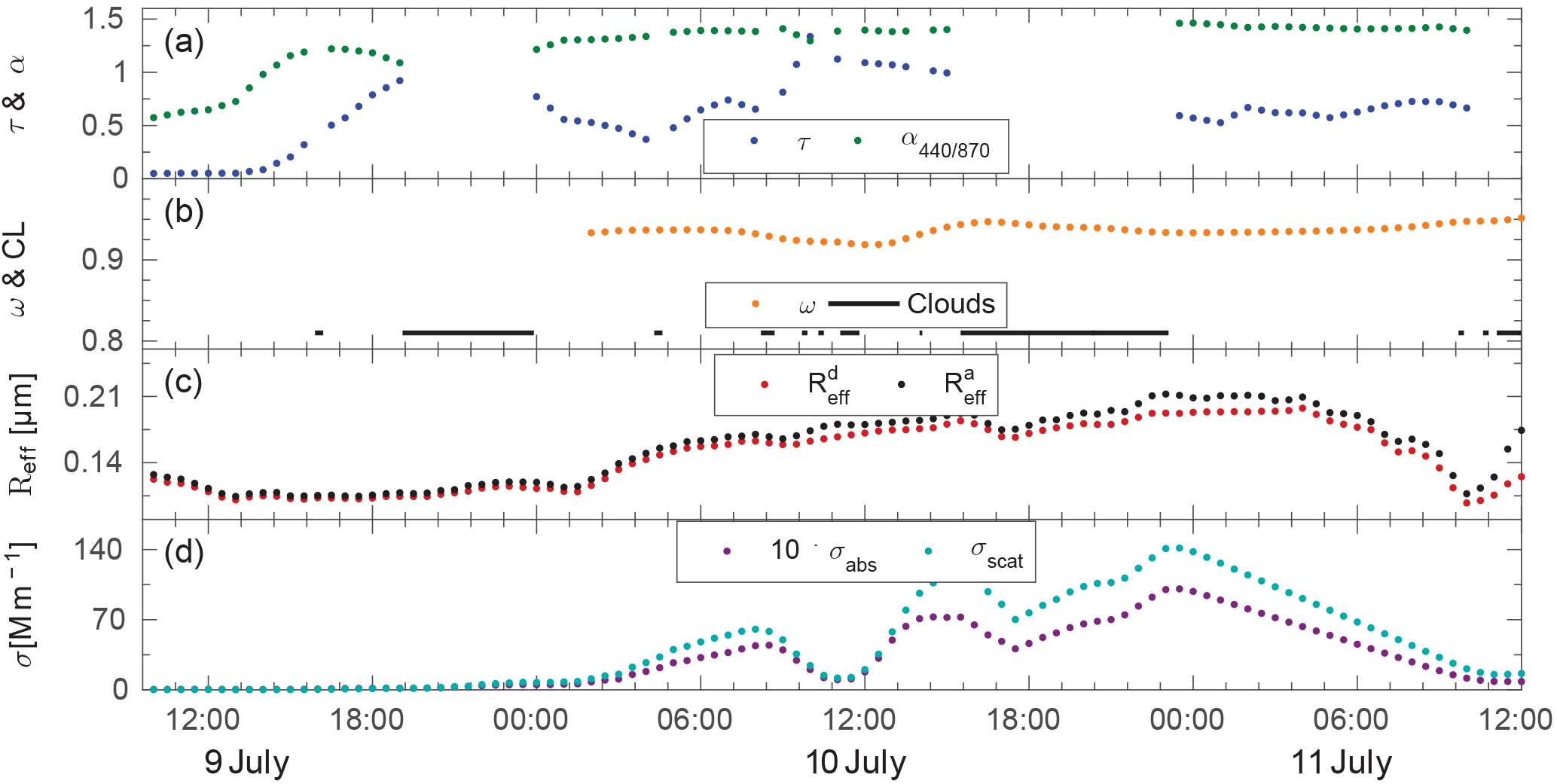
Figure 1 Temporal variability in aerosol single-scattering properties during the BB2015 event over Ny-Ålesund, in particular aerosol optical depth τ at 530 nm (blue dots) and Ångstrom exponent α (green dots) measured by SP1a (a), single-scattering albedo ω^d at 530 nm (yellow dots) calculated from in situ data and cloud coverage (black line) from the pyranometer (b), effective radiuses at dry $R_{\mathrm{eff}}^{\mathrm{d}}$ (red dots) and ambient $R_{\mathrm{eff}}^{\mathrm{a}}$ (black dots) conditions measured by SMPS and APS (c), and absorption coefficient σ_abs multiplied 10 times (purple dots) and scattering coefficient σ_scat (light blue dots) at 530 nm, obtained from the PSAP and nephelometer.

3 Results

3.1 The temporal variability in aerosol single-scattering properties during the BB event at Ny-Ålesund

In July 2015 the transport of a BB plume over the Arctic region was observed, being advected from the intense tundra and boreal forest fires in the northern regions of North America. The plume altered both the optical and microphysical properties of aerosols, as indicated by the in situ and ground-based remote sensing instruments installed at Ny-Ålesund. Thus, τ conditions characteristic of summer conditions (mean summer τ=0.08) were enhanced with a factor of 10, making it the strongest event in the past 25 years (Markowicz et al., 2016a). Markowicz et al. (2016a) reported the development and further intensification of tundra fires in Alaska, introduced by a series of frequent lightning strikes occurring from mid-June to late July 2015. The transport of the BB plume was visible between 4 and 6 July, from the central part of Alaska, via the North Pole, to the Spitsbergen. Starting in the afternoon of the 9 July, until approximately noon on 11 July, the BB plume was visible at Ny-Ålesund, as indicated by in situ and remote sensing instruments (Fig. 1). As suggested by the lidar data by Markowicz et al. (2016a), this advection lasted longer in the area of study; however, the appearance of clouds around noon on the 11 July (Fig. 1b) terminated further measurements.

Although Markowicz et al. (2016a) reported the beginning of the event at 14:00 UTC, based on the lidar data, we see a temporal discrepancy between in situ and remote sensing measurements of half a day, resulting from transport taking place in the mid-troposphere (Fig. 1d). The ultimate manifestation of a BB plume at the surface, however, might be evidence of a turbulent vertical mixing.

The event was characterized by the mean τ₅₅₀ value estimated at the level of 0.64, with a maximum reaching as high as 1.2 at noon on 10 July (Fig. 1a). The temporal variability in α was rather low, with an average value of around 1.5 throughout the advection, which indicates the existence of mostly fine particles. This hypothesis is confirmed by the aerosol size distribution measured at ground level, which shows that particles are mainly distributed in the accumulation mode during the BB event (Moroni et al., 2017).

The mean ω^d at 530 nm obtained for the event is 0.94 ± 0.02 (Fig. 1b), indicating moderate absorbing properties, characteristic for aged BB plumes. Note that the value is slightly higher than in situ ω^d reported by Moroni et al. (2017), of 0.91, resulting from the applied additional multiple-scattering correction to PSAP data in this study. During the most intense period ω^d reduces to 0.9. Aerosol absorbing properties decrease over the event, resulting in an increase in ω^d on 11 July to its maximum value of 0.95. Lund Myhre et al. (2007) presented results from the transport of smoke-enriched air masses over Ny-Ålesund. The episode was very similar to the one under study, as the mean τ₅₀₀ reached the value of 0.68 with a mean ω of 0.98, after 7 days of transport from central Europe. It is clearly visible that ω is slightly higher by comparison to the 2015 BB event (labelled BB2015). Apart from the above paper, the representation of BB plumes lasting in the atmosphere for more than 3 days, in literature, is rather rare. Reid et al. (2005) reported a number of mean surface ω, characterizing aged BB plumes ranging from 0.76 to 0.93, from various in situ measurements. Although values usually seem to be much lower by comparison to the BB2015 event, the differences result from the definition of aged plumes. In the mentioned Reid et al. (2005) paper, aged aerosol was characterized as a plume existing in the atmosphere for more than 24 h only; while in this study, its persistence is much longer, at around 7 days.

The mean value (14:00 9 July–11:30 11 July) of absorption coefficient (σ_abs) was 4.0 Mm⁻¹, while extinction coefficient (σ_ext) was 65.0 Mm⁻¹, as indicated by in situ instruments (Markowicz et al., 2016a) during BB2015. Reported extensive optical properties of aerosols significantly exceeded their typical annual mean values (σ_scat: 4.35 Mm⁻¹, σ_abs: 0.18 Mm⁻¹; α: 1.15), characterized by Schmeisser et al. (2018) for the station at Mount Zeppelin (475 m a.s.l.), located close to Ny-Ålesund.

We obtained average values of 0.17 ± 0.02 and 0.18 ± 0.02 µm for effective radius at dry ($R_{\mathrm{eff}}^{\mathrm{d}}$) and ambient ($R_{\mathrm{eff}}^{\mathrm{a}}$) conditions, respectively (Fig. 1c). Presented results are in good agreement with studies provided by Nikonovas et al. (2015), who reported the values of $R_{\mathrm{eff}}^{\mathrm{a}}$ originating from open shrublands to be as high as 0.176–0.194 µm. $R_{\mathrm{eff}}^{\mathrm{a}}$ being in the lower boundary of the class reported by Nikonovas et al. (2015) is likely to result from the chemical composition of the smoke plume, which does not allow for intense hygroscopic growth of aerosols (consisting mainly of hydrophobic particles; Moroni et al., 2017). We may also speculate that it is due to the efficiency of the scavenging processes with a much longer transport.

Figure 2 Vertical profiles of aerosol single-scattering properties at 530 nm on 10 and 11 July 2015 (UTC), based on the lidar measurements, radio-sounding profiles, and model output (lines), as well as in situ measurements (dots). Subfigures include lidar-derived (LID) extinction coefficient at ambient (${\mathit{\sigma }}_{\mathrm{ext}}^{\mathrm{a}}$; green) and dry (${\mathit{\sigma }}_{\mathrm{ext}}^{\mathrm{d}}$; blue) conditions, as well as absorption coefficient σ_abs multiplied 10 times (red; a_1–4), modelled extinction profile from GEM-AQ (GEM ${\mathit{\sigma }}_{\mathrm{ext}}^{\mathrm{a}}$; b_1–4), retrieved single-scattering albedo ω^a (c_1–4) at ambient conditions, radio-sounding profiles of relative humidity RH (d_1–4), and potential temperature θ (e_1–4). Blue transparent layers denote temperature inversions (T_inv).

Additionally, Markowicz et al. (2016a) present a significant increase of up to 2.2 cm in the precipitable water (PW); This is rather unusual in the High Arctic. The advection of such humid air masses may significantly enhance the water uptake of aerosols, hence their scattering properties. Using in situ instruments, that dry the particles (RH usually of around 15 % in the chamber), possibly leads to an appreciable underestimation of aerosol scattering, and thus radiative properties.

3.2 Retrieval of the single-scattering properties at ambient conditions

An analysis regarding the identification of a source region was performed by means of the GEM-AQ model. We investigated the path of smoke back-trajectories, transported across the Arctic region (not shown), and confirmed that the studied BB plume originated from wildfires over Alaska. Both the timing and inflow of aerosol-enriched air masses and the rapid increase in τ₅₅₀ support the above statement. Vertical profiles of PM₁₀ demonstrated polluted air masses extending up to approximately 3 km, with maximum mass mixing ratios reaching 35 ppb at 2 km. Analysis of 3-D extinction fields over Svalbard revealed a thick layer, with higher values above the PBL (Fig. 2b_1–4). The model reproduced the altitude of elevated extinction coefficients; however, the complex vertical stratification was not captured by the model due to sparse vertical resolution.

In this section, we present example results of the applied methodology concerning the retrieval of a ω^a profile. The first case (11:30 10 July; Fig. 2a₁–e₁), in terms of ${\mathit{\sigma }}_{\mathrm{ext}}^{\mathrm{a}}$ profiles, represents the moment of maximum τ value, while cases 2–3 indicate average conditions, characterizing the BB plume (23:00 10 July; Fig. 2a₂–e₂; 02:30 11 July; Fig. 2a₃–e₃). The last chosen case outlines the transition of the atmosphere – with intensified atmospheric dynamics, an appreciable turbulent mixing, and convective cloud formation – to the conditions where a formation of low clouds relying on stable conditions is visible; thus it is likely that vertical mixing is gradually suppressed.

The vertical profiles of thermodynamic variables, such as RH and potential temperature (θ), were retrieved from two radio soundings performed on the 10 and 11 July, around noon. On the 10 July, the θ profile indicates the existence of two rather thick inversion layers at around ground level and at 3.5 km, as well as an almost isothermal layer at 2–3.5 km (Fig. 2e_1–2). The profiles on the 11 July revealed that all layers were attenuated during the day and were significantly lifted (Fig. 2e_3–4). The appearance of additional thin inversions, together with a visible decay in θ lapse rate and the mentioned transformations of previous layers, suggest the existence of vertical mixing. A similar vertical structure is visible in RH profiles with values oscillating around 15–90 %. A significant decay in RH values is attributed to θ inversion layers; in between, however, the values usually exceed 75 %.

The vertical structure of ${\mathit{\sigma }}_{\mathrm{ext}}^{\mathrm{a}}$ (Fig. 2a_1–4) retrieved from the lidar observations is strongly dependent on both θ and RH profiles. The latter designates the enhancement of ${\mathit{\sigma }}_{\mathrm{ext}}^{\mathrm{a}}$ inside the visible layers, attributed to hygroscopic growth of aerosols, while θ determines their thickness. Overall, the smoke plume is visible from around ground level to 3.5 km. However, the shape of the lower boundary is uncertain, due to the lidar overlap issue under 0.7 km. The ${\mathit{\sigma }}_{\mathrm{ext}}^{\mathrm{a}}$ inside the smoke layer ranges from 100 to 350 Mm⁻¹, with a significant vertical variability. In all cases an additional secondary ${\mathit{\sigma }}_{\mathrm{ext}}^{\mathrm{a}}$ enhanced layer is visible above the main BB plume. In case 1 it is visible at around 5.5 km, and is likely to be connected with the existence of thin clouds of marginal meaning in light of the smoke plume itself. In the remaining cases, secondary layers which are visible at 3.5–4.5 km may be the residuum of cumulus clouds, reported by Markowicz et al. (2016a), resulting in mixing processes between smoke and the air layer above the BB plume. In Fig. 2a_1–4 the vertical variability of retrieved ${\mathit{\sigma }}_{\mathrm{ext}}^{\mathrm{d}}$ and σ_abs are additionally presented. The ${\mathit{\sigma }}_{\mathrm{ext}}^{\mathrm{d}}$ represents the result of Eqs. (3)–(6), where the hygroscopic growth of aerosol is removed.

The calculated profiles of ω^a vary from 0.93 to 0.96. In the presented cases, ω^a profiles shift towards less absorbing properties and as a result of the applied approximation (in particular Eq. 6), its vertical structure reflects the vertical variability in RH.

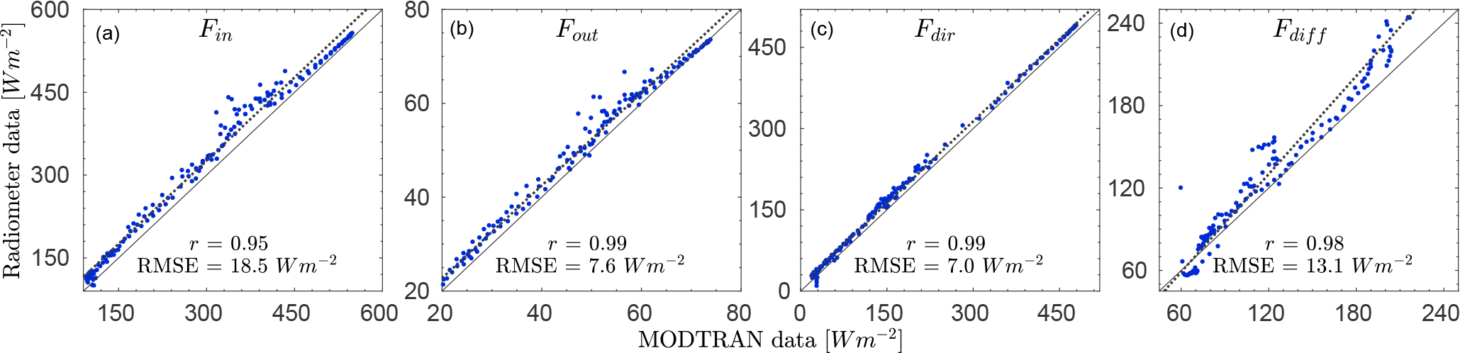
Figure 3 Comparison of model-derived and measured irradiances, in particular incoming F_in (a), outgoing F_out (b), direct F_dir (c), and diffuse F_diff (d) surface fluxes on 9–11 July 2015. The solid black lines refer to the perfect fir, dotted black lines to a linear fit, r refers to the Pearson correlation coefficient, and RMSE represents the root mean square error.

3.3 Comparison of model-derived irradiances with the measurements

Figure 3 presents the results of the performance of MODTRAN simulations compared with in situ measurements, in terms of radiative properties of the atmosphere. The Pearson correlation coefficients for MODTRAN and radiometer data exceed 0.95 for all radiation components (in particular total incoming F_in – 0.95, outgoing F_out – 0.99, direct F_dir – 0.99, diffuse F_diff – 0.98 fluxes at the surface), suggesting a well-defined statistical dependence of the variables. Nevertheless, the model seems to slightly underestimate all fluxes with regard to measurement data, especially visible in F_diff. The root mean square error (RMSE) is estimated at the level of 18.5 and 7.6 W m⁻² for F_in and F_out. The mean bias of total incoming flux at the surface is mainly related to RMSE of F_diff, being as high as 13.1 W m⁻². The F_dir RMSE is almost 2 times lower than the latter and reaches 7.0 Wm⁻². This difference in biases of F_dir and F_diff result from the distinction in parameters governing both irradiances, in particular F_dir is a function of parameters that are measured with good accuracy (τ and PW), while F_diff is additionally controlled by variables with appreciably higher uncertainty (ω, phase function, surface albedo, etc.).

Although cloud-contaminated radiometer data were previously removed, higher RMSEs together with relatively high temporal variability in F_diff, which is a significant function of the cloud coverage, might suggest that the performance of cloud-screening algorithm was insufficient for the case under study. Therefore, presented results from in situ data should be used with caution, bearing in mind that they may occasionally represent all-sky conditions.

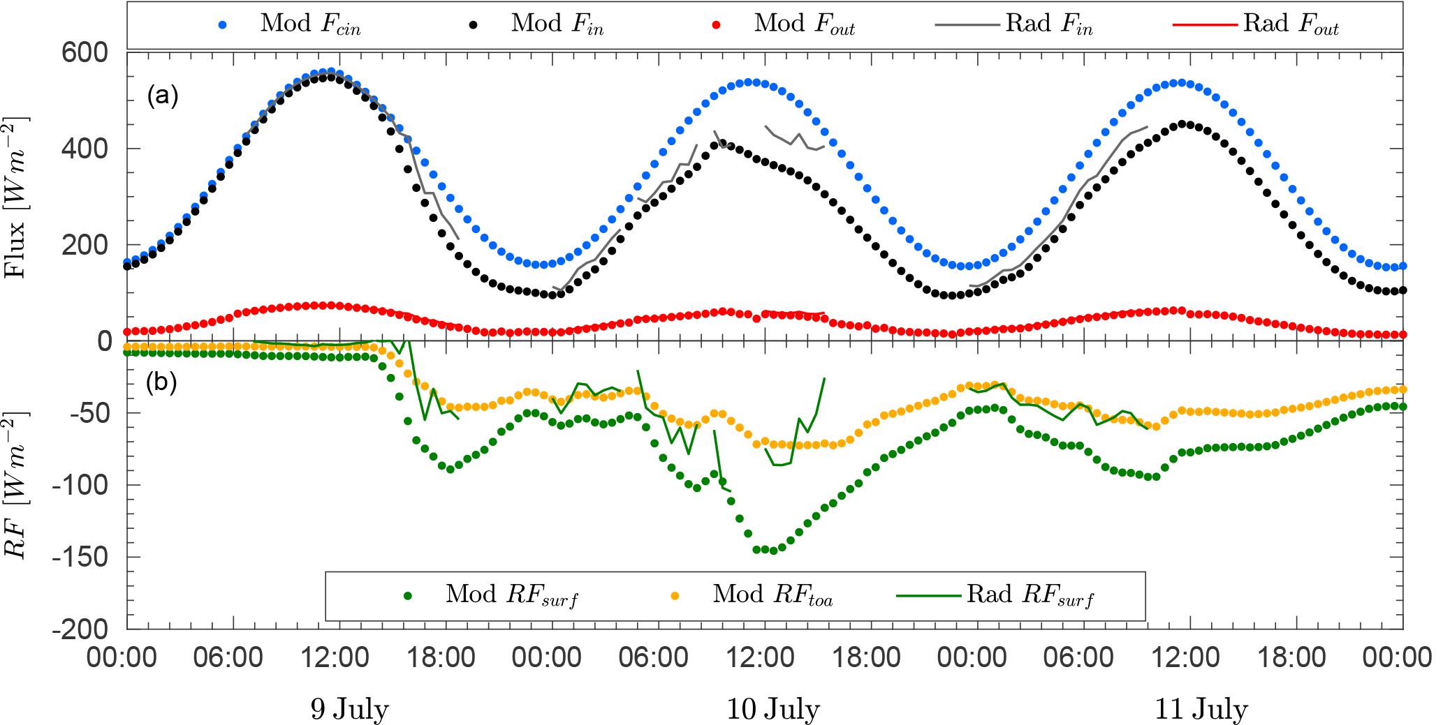
Figure 4 Temporal variability in (a) the surface radiation fluxes: total incoming flux at the polluted case F_in (black) and at the clean case F_cin (blue), as well as total outgoing flux at the polluted case F_out (red), simulated by MODTRAN (dots), and measured by radiometers (lines). The gaps in the radiometer data refer to the cloud contamination. Panel (b) presents radiative forcing at the surface RF_surf (green) and at the top of the atmosphere RF_toa (orange).

3.4 Temporal variability in radiative forcing at Ny-Ålesund

Results presented in this chapter were previously introduced in Sect. 2.3.4 concerning ω^a and g^a retrievals. To estimate the overall performance of the mentioned approximation, we performed two initial simulations that assumed fixed values of all optical and microphysical properties of aerosol, except for ω and g. In the first, we used ω^d and g^d measured by in situ instruments, while the second applied ω^a and g^a approximations. Differences between the two simulations indicated the decrease in RF (in absolute magnitude), on average by about 3.1 W m⁻² for the BB event (14:00 9 July–11:30 11 July), when ambient conditions were used. This was due to an increase in both F_in and F_out by 3.5 and 0.4 W m⁻², respectively, for the simulation with aerosol included. The impact of the retrieval on enhancement of F_in and F_out might be vastly attributed to ω correction, with the influence of 81 %, and only 19 % to g^a approximation.

Figure 4 presents the comparison of temporal variability of irradiances (Fig. 4a) and clear-sky RF (Fig. 4b). The daily variability in total incoming flux in the clean case (F_cin) is mainly a function of the solar zenith angle and for the 9–11 July 2015 ranges from around 153.0 W m⁻² at midnight to 560.8 W m⁻² at noontime. On the other hand, F_in is additionally strongly affected by the optical and physical properties of the advected smoke. The model's performance at background conditions might be validated at the period between 07:00 and 14:00 UTC on 9 July. This represents the clear-sky period with an infinitesimal load of aerosols, typical for summer background conditions in the Arctic. Both measured by radiometer (hereinafter referred to as Rad) and modelled by MODTRAN (hereinafter referred to as Mod) F_in are in rather good agreement, deviating on average by only 9.7 W m⁻² (2 %) from each other. The existence of aerosol indicates the mean decrease in F_in by 0.4 % (Rad F_in), as well as 2.3 % (Mod F_in), as compared to the mean value of F_cin (07:00 to 14:00 UTC on 9 July). Measured and modelled F_out indicate a very good agreement with a difference of less than 1 %, reaching on average 69.8 W m⁻² (Rad) and 69.4 W m⁻² (Mod).

At 14:00 UTC Markowicz et al. (2016a) reported an advection of the BB plume over Ny-Ålesund, characterized by a complicated structure of the BB layers, with a mixture of aerosol and clouds. Since the mean value of Mod F_in during the event (14:00 9 July–11:30 11 July) is estimated at the level of 243.0 W m⁻², the existence of the BB aerosol reduced the incoming flux, on average by around 90 W m⁻², when compared to the case represented by summer background conditions (332.1 W m⁻²; 07:00 to 14:00 UTC on 9 July). Furthermore, we report the mean value of outgoing irradiance (Mod F_out) reaching 36.9 W m⁻². The highest decrease in Mod F_in is visible on 10 July as indicated by the observed maximum of τ₅₅₀ during the BB event. The reduction of Mod F_in exceeded 27 % for the summer background conditions (compare 07:00–14:00 UTC on 9 and 10 July). Additionally, a higher temporal variability in Rad F_in at the time, with respect to the previous day, is observed. It is likely to result from both a possible BB aerosol activation and increased turbulence. Further to this, a number of high- and mid-level cumulus clouds are reported around noon and in the afternoon (Markowicz et al., 2016a), which support the above statement.

RFs_surf were estimated by means of two approaches: in the first approach, we used MODTRAN (Mod RF_surf) simulations to account for both terms (representing polluted and clean cases; for details see Sect. 2.1) in the following equation:

$$\begin{array}{}\text{(12)}& {\mathrm{RF}}_{\mathrm{surf}}=(F_{\mathrm{in}}-F_{\mathrm{out}})-(F_{\mathrm{cin}}-F_{\mathrm{cout}}),\end{array}$$

where F_cout is total outgoing flux at the surface, simulated in the clean case. In the second approach, the radiometer data were used in place of the polluted case simulated by MODTRAN RTM. Since the second term of Eq. (12) is identical in both RFs_surf approaches, the mean discrepancies between Mod and Rad RFs_surf, exceeding 30 % during the event, relate to differences in Mod and Rad F_in (in particular F_diff). Further to this, the 3-D effects of the surface, the uncertainty in the radiometers enhanced by high solar zenith angles, and the approximations used for the model of aerosol optical properties in the RTMs may play a major role. We report the average radiative forcing at the surface (RF_surf) of the studied smoke plume (14:00 9 July–11:30 11 July) at the levels of −78.9 W m⁻² (Mod) and −43.3 W m⁻² (Rad), indicating a significant cooling effect of BB aerosol at the surface. Radiometer data represent all-sky conditions, since the discussed BB event is extremely complicated and therefore a possible cloud contamination seems impossible to separate entirely. However, periods with a clear influence of clouds were removed (i.e. 15:00–21:00 10 July), therefore the presented mean value of Rad RF, lacks the most intense period (see Fig. 4b). The highest values (in absolute magnitude) are observed at around 12:00 UTC on 10 July, being attributed to the highest values of τ₅₅₀, as previously mentioned; thus, a momentary Mod RF_surf exceeded −147 W m⁻² regarding MODTRAN simulations. Similar results were reported by Stone et al. (2008), who studied smoke advected from Alaska to the Canadian Arctic during 2 July 2004. The authors came to the conclusion that an average diurnal τ₅₀₀ of 0.5 would produce a cooling effect at the surface, reaching 40 W m⁻². Since in our case the average τ₅₅₀ is 0.64, the results seem to be complementary. On the other hand, a study from Sitnov et al. (2013) revealed smaller absolute values of RF_surf at much higher τ₅₅₀ for the wildfires observed in European Russia at the beginning of August 2010. For the average τ₅₅₀ between 0.98 and 1.16, the authors estimated RF_surf to be around −60 W m⁻². As RF_surf is a function of the solar zenith angle (Stone et al., 2008) and the duration of the insolation, as well as surface albedo (Carslaw et al., 2010), the discrepancies between these variables might be the explanation of the reported differences.

The average value of Mod RF_toa exceeded −47.0 W m⁻², indicating that the BB plume cooled the entire atmospheric column. Within the atmosphere, however, it has a positive impact of 31.9 W m⁻² (Mod RF_atm). This pattern is in agreement with Myhre et al. (2013b) and Stone et al. (2008), who also reported negative values at the TOA and positive ones when an atmospheric layer is considered. High single-scattering albedo values and negative RF_toa clearly show that scattering is dominant with respect to the contribution of the light absorption. Indeed, absorption species (mainly BC) are able to mitigate the cooling effect of the BB event in the atmosphere, but not sufficiently to change the RF sign at the TOA. This means that BC particles play a minor role with respect to scattering particles (sulfate; organic carbon, OC; etc.). This could also be demonstrated by the changes in atmospheric concentrations of BC, OC, and sulfate aerosol, measured at Gruvebadet. In particular, the relative concentrations increase about 20 times for BC and OC, and about 10 times for non-sea-salt sulfate during the BB event, with respect to the background level. In spite of the BC and OC, relative increases are similar; the absolute concentrations of OC are more than 10 times higher than atmospheric concentration of BC (Moroni et al., 2017). Overall, the described RF of the plume had an about 31 % higher (in absolute magnitude) influence at the surface, in comparison with the TOA. Model calculations usually overestimate Mod RF_surf values, which on average, deviate from Rad RF_surf by around 32.9 %, possibly related to all-sky conditions being represented by radiometer measurements that increase diffusive flux.

The mean estimated radiative forcing efficiency at the surface (Mod RFE_surf) of the BB event in Svalbard of −126 W m${}^{-\mathrm{2}}/{\mathit{\tau }}_{\mathrm{550}}$ is slightly higher than other estimates of smoke transport, such as −99 W m${}^{-\mathrm{2}}/{\mathit{\tau }}_{\mathrm{550}}$ reported by Markowicz et al. (2016b) for the Canadian forest fires advection over Europe in 2013, and −88 W m${}^{-\mathrm{2}}/{\mathit{\tau }}_{\mathrm{550}}$ for wildfires observed over Crete, Greece in 2001 (Markowicz et al., 2002). On the other hand, multiyear mean RFE_surf values obtained for different regions are appreciably higher, i.e. RFE_surf originating from tropical forest fires over the Amazon basin is estimated at the level of −140 ± 33 W m${}^{-\mathrm{2}}/{\mathit{\tau }}_{\mathrm{550}}$, while boreal forest fires from North America are as high as −173 ± 60 W m${}^{-\mathrm{2}}/{\mathit{\tau }}_{\mathrm{550}}$ and RFE_surf for African savannahs are at the level of −183 ± 31 W m${}^{-\mathrm{2}}/{\mathit{\tau }}_{\mathrm{550}}$ (García et al., 2012). The reported discrepancies are a function of the solar zenith angle, surface albedo, and single-scattering properties of aerosols. In general, more efficient RFEs_surf are characterized by smoke plumes with lower values of ω, i.e. 0.85 and 0.91 for African savannahs and the Amazon forest, respectively (García et al., 2012). Although ω values are similar for the case under study, i.e. boreal forest, the latter is more efficient due to a higher solar zenith angle.

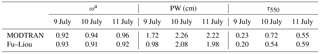
Table 2 The mean daily values of the single-scattering albedo ω^a, precipitable water PW (cm), and aerosol optical depth τ₅₅₀ at 550 nm used as inputs to MODTRAN and Fu–Liou simulations.

3.5 The comparison of RF derived from MODTRAN and Fu–Liou simulations

This section focuses on the comparison of RFs simulated by the MODTRAN and Fu–Liou models. The results of the latter were previously published in Markowicz et al. (2017b) regarding the transport of this BB plume over the Northern Hemisphere. In the following section, all RFs were retrieved over the ocean area, near Ny-Ålesund (78.5^∘ N, 9.5^∘ E), assuming a spectral surface albedo of the Fresnel reflection over a water body to eliminate discrepancies in the surface properties from our investigation.

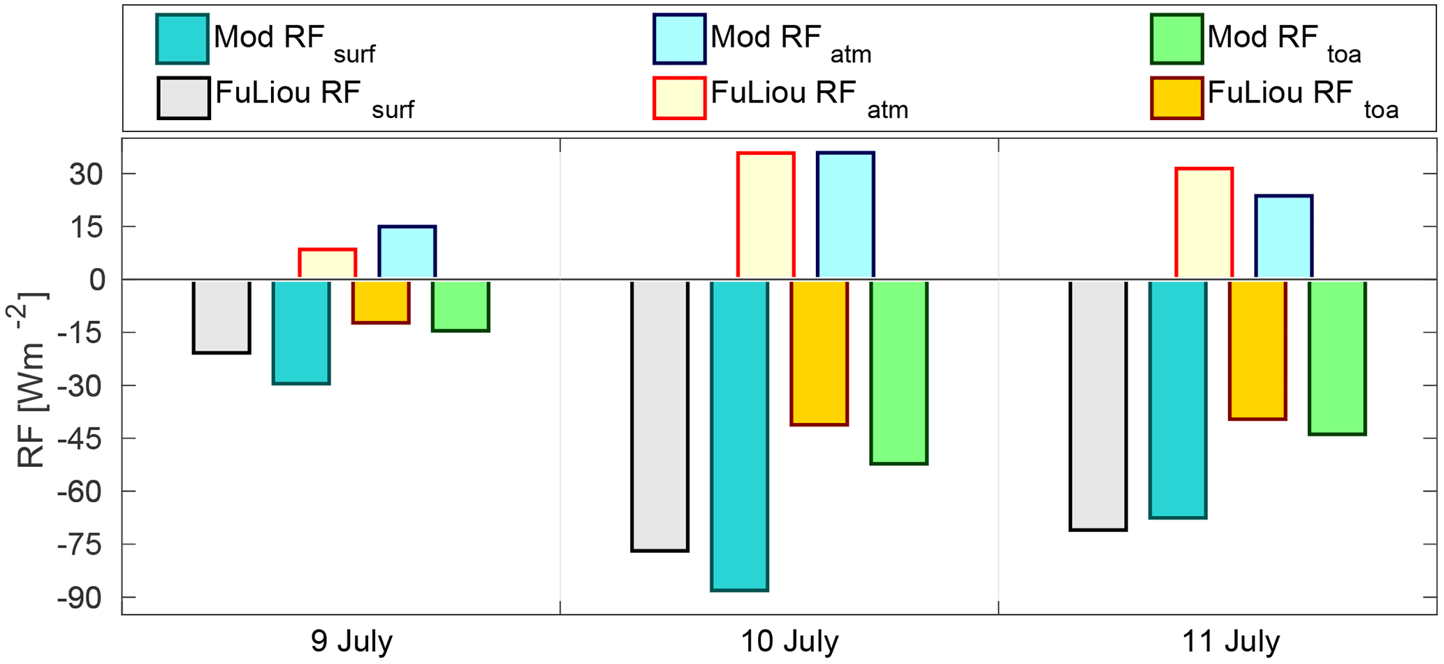
Figure 5 The mean daily values of radiative forcing (RF) calculated by means of Fu–Liou (FuLiou) and MODTRAN (Mod) models. Simulations were run for clear-sky conditions at the surface (subscript “surf”), within the atmosphere (subscript “atm”), and at the top of the atmosphere (subscript “toa”). The surface reflectance in MODTRAN simulations is based on the Fresnel reflection calculations at the ocean surface.

Table 2 presents the comparison between input variables to both models: mean daily ω^a, PW, and τ₅₅₀. Column-integrated Mod ω^a is calculated yielding (Schafer et al., 2014):

$$\begin{array}{}\text{(13)}& {\mathit{\omega }}^{\mathrm{a}}={\displaystyle \frac{\underset{\mathrm{0}}{\overset{\mathrm{10}\mathrm{km}}{\int }}{\mathit{\sigma }}_{\mathrm{ext}}^{\mathrm{a}}\left(z\right)\cdot {\mathit{\omega }}^{\mathrm{a}}\left(z\right)\mathrm{d}z}{\mathit{\tau }}},\end{array}$$

while ω^a in the case of MODTRAN simulations having an increasing trend (from 0.92 to 0.96) within 9–11 July, the same quantity shows 3–6 % more absorbing properties, and is rather constant for Fu–Liou calculations oscillating around 0.91–0.93. The same trend is visible for PW mean values, where it is between 1.72 and 2.26 cm for MODTRAN simulations; however, for Fu–Liou it is 10–40 % lower. Additionally, the retrieved mean MODTRAN τ₅₅₀ equal to 0.23–0.72 and a Fu–Liou value of 0.2–0.59 seem to deviate from each other by 8–35 %. Furthermore, while the highest τ₅₅₀ value for MODTRAN simulations is on 10 July, it is more noticeable on 11 July for the Fu–Liou simulations. Presented discrepancies between variables are satisfactory, given the fact that the Fu–Liou model has larger spatial resolution.

Figure 5 presents the daily mean values of RFs derived from MODTRAN and Fu–Liou calculations for the BB event at the surface, within the atmosphere (RF_atm), and at the TOA for clear-sky conditions. Overall, the difference between daily mean values of MODTRAN and Fu–Liou simulations is, on average, close to around 15 %, with all assumed input variables and calculated RFs being lower for the latter (with the exception of RF_atm). Differences between MODTRAN and Fu–Liou simulations are vastly connected with slightly different aerosol optical properties. Considering that for each model, different resolutions of input parameters over the slightly distinct area were used, the authors consider the obtained accuracy to be fairly good.

Given the fact that RF_toa for all-sky conditions modelled by Fu–Liou is equal to −14.0 W m⁻² (not shown) on 10 July, these results are considered exceptional in the Arctic records, being of a similar magnitude to other investigations on high aerosol load events in this region. All-sky RF_toa for the BB transport from Europe in 2006 was estimated between −12 and 0 W m⁻² (Lund Myhre et al., 2007).

3.6 3-D effects on RF at the surface in the vicinity of Kongsfjorden

In the previous sections, we discussed the RF computed for a single cell, using measurements from Ny-Ålesund as input data. In that approach, called the plane-parallel (PP) approach, the Earth's surface was assumed flat and uniform, and the atmosphere was horizontally uniform. Thus, both topographic effects (shading, slope inclination, etc.) and small-scale (subgrid) variability in surface albedo were neglected. Moreover, net photon transfer between the atmospheric column over the cell and the adjacent atmosphere was assumed zero. In this section, however, the above effects are taken into consideration. 3-D geometry and 3-D Monte Carlo simulations of radiative transfer were used to analyse RF surface variability and thus, uncertainty resulting from single-cell radiative transfer schemes in the vicinity of Konsfjorden.

The simulations were performed for a single wavelength λ=469 nm and the solar position for the time of the retrieval of the aerosol properties profile (10 July 2015 11:30 UTC; solar zenith angle = 57^∘, solar azimuth = 173^∘). We performed two simulations, one with and one without 3-D effects. In the former simulation we used the 3-D Monte Carlo code with the “real” topography (the real surface reflective properties, changeable within the domain). In this approach photons can travel freely in the 3-D atmosphere. In the simulation without 3-D effects, RF was computed using the plane-parallel geometry for each of the individual 200 m cells/columns. In this method the Earth's surface is assumed flat, horizontally within each column but both the land elevation and the reflective properties of the surface vary from cell to cell. Further to this, the atmospheric columns are independent from each other, i.e. horizontal photon exchange between columns is neglected; thereby neither optical properties of the surface and atmosphere nor topography of adjacent cells influence surface radiative forcing in a given column. Using the plane-parallel approach for RF computations for a single atmospheric column or for a group of columns may lead to biased results.

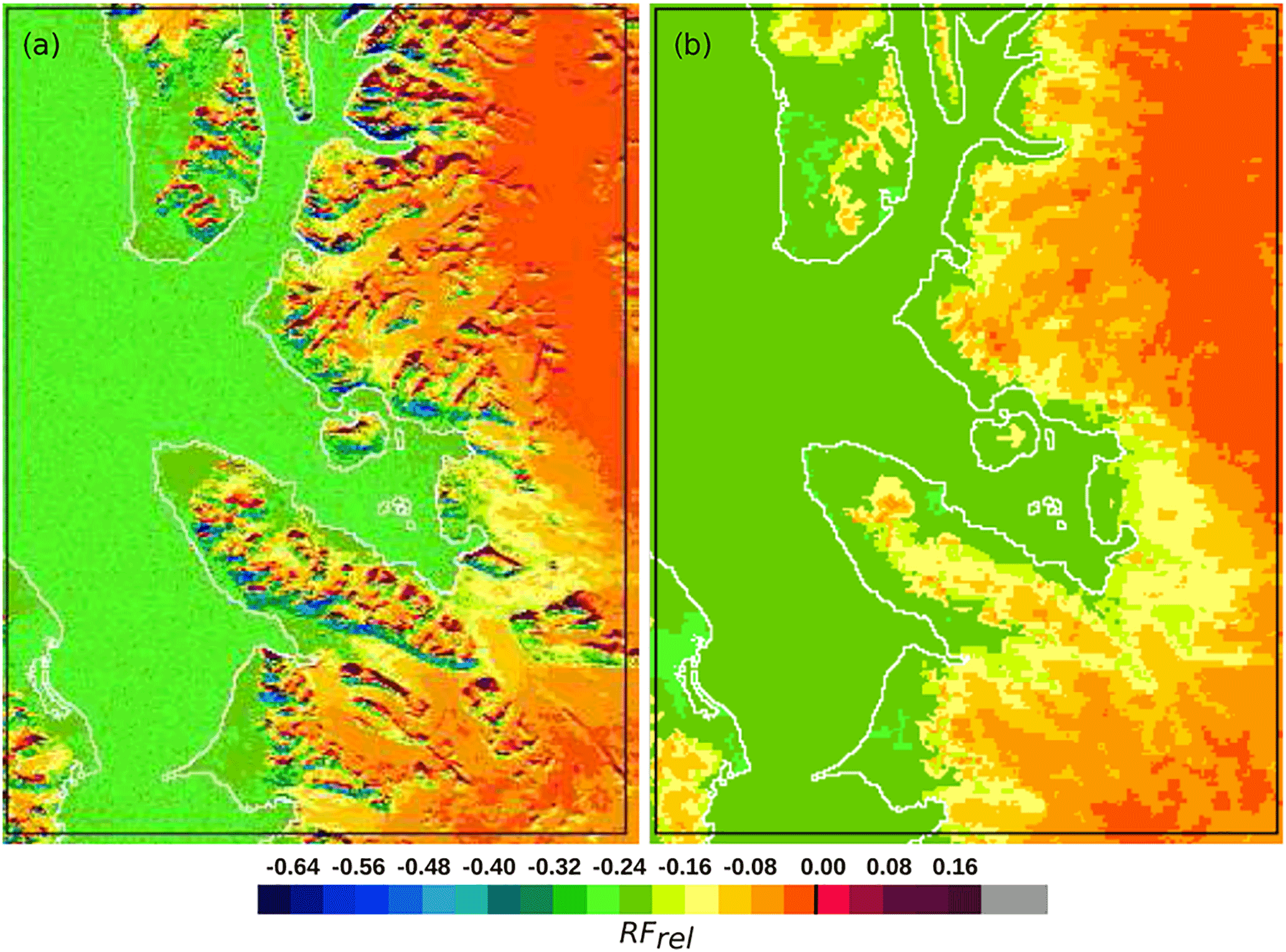
Figure 6 A comparison of the RF_rel spatial variability at the Earth's surface derived from the 3-D Monte Carlo model (a) with RF${}_{\mathrm{rel}}^{\mathrm{pp}}$ spatial variability (b) computed, applying the Monte Carlo model with plane-parallel geometry to each column independently. In panel (b) both the surface topography and photon exchange between adjacent columns are neglected. Computations for λ=469 nm, solar zenith angle = 57^∘, solar azimuth = 173^∘, and aerosol properties of 10 July 2015, 11:30 UTC.

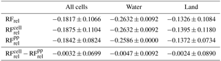
Table 3 Mean relative radiative forcing RF calculated concerning the actual surface, RF_rel, and the horizontal cell surface RF${}_{\mathrm{rel}}^{\mathrm{cell}}$ using the 3-D Monte Carlo model. RF${}_{\mathrm{rel}}^{\mathrm{pp}}$ is RF computed, using the plane-parallel geometry to each column independently. Computations were done for λ=469 nm, solar zenith angle = 57^∘, solar azimuth = 173^∘, and aerosol properties of the 191st day of 2015.

In this section, RF is expressed as a fraction of downward irradiance at the TOA (Eqs. 9–11). Further in this section, we will skip λ and RF_rel, RF${}_{\mathrm{rel}}^{\mathrm{cell}}$ and RF${}_{\mathrm{rel}}^{\mathrm{pp}}$ will denote relative spectral RF, simulated using the 3-D modelling, RF_rel (λ=469 nm), RF${}_{\mathrm{rel}}^{\mathrm{cell}}$ (λ=469 nm), and the plane-parallel approach to individual cells, RF${}_{\mathrm{rel}}^{\mathrm{pp}}$ (λ=469 nm).

Figure 6 shows the spatial distribution of RF_rel (Eq. 10) at the surface and compares it to the distribution derived using the plane-parallel geometry to each column independently. The mean values of RF and the standard deviations are compared in Table 3. In the analysed case, the domain mean values and standard deviation of RF_rel is −0.1817 ± 0.1066 for the RF calculated with respect to the real inclined surface (i.e. per unit area of the inclined surface; compare Eqs. 9–10), and RF${}_{\mathrm{rel}}^{\mathrm{cell}}$ is −0.1875 ± 0.1104 when the RF is calculated with respect to the horizontal cell surface (i.e. per unit area of the cell surface; compare Eq. 11). There is a large difference between the RF over water and land surfaces, which is mainly due to differences in surface albedo between these regions. An absolute value of RF is smaller and weakly variable over the fjord surface, where mean RF${}_{\mathrm{rel}}^{\mathrm{cell}}$ is equal to mean RF_rel and reaches −0.2632 ± 0.0092. Its coefficient of variation is 3.5 %. The actual value of RF variability over the sea may be even lower, because the noise of the Monte Carlo method may enhance it. Being a probabilistic technique where photons are traced on their random paths through the atmosphere, Monte Carlo is associated with random noise. The land RF is characterized with both RF${}_{\mathrm{rel}}^{\mathrm{cell}}$ and RF_rel less negative mean values of −0.1395 ± 0.1180, and −0.1326 ± 0.1084, respectively, and much stronger surface variability. The respective coefficients of variation are 84.6 and 81.7 %.

In our simulation, the variability in RF over the sea is caused by the impact of the surrounding land only. Apart from shading the sky and sun by the orography, the spatial variability in RF and its deviations from the plane-parallel RF values, are caused by positive net horizontal photon transfer from the land area. Horizontal photon transfer due to reflection between the atmosphere and the underlying surface is efficient over bright areas, such as snow-covered land and glaciers. The horizontal distance of the photon transmission outside the bright underlying surface, related to the effective height at which the radiation reflected upward by the Earth's surface, is reflected downward by the atmosphere. The net horizontal transport is observed for both atmospheres, with and without aerosols, but in each case the effective height of reflection is different. An appearance of a dense, low-lying aerosol layer reduces the effective reflection height, and thus the horizontal distance the photons can travel over the fjord; but at the same time, it intensifies the reflectance of the atmosphere, compared to the clean case. Therefore, the gradient in irradiance, with distance from the reflective land, is stronger in the polluted case. The atmosphere without aerosols acts similarly to a very thin cloud located higher over the Earth's surface, while the aerosol layer can be compared to a thicker cloud with its base at a lower height (Rozwadowska and Górecka, 2012).

The main factors influencing RF and its variability over land in the vicinity of Kongsfjorden are reflective properties of the land surface, slope exposition of the sun, and shading of the sun by the mountains. The impact of photons reflected from nearby sunlit slopes and horizontal photon transport due to multiple reflections between the sky and the surface on RF variability are of secondary importance over the land.

In the analysed case, the highest magnitude of negative RF was found for sun-facing slopes of white sky albedo (calculated from diffusive component only) of around 0.2. In such places, the effective solar zenith angle is relatively low and a high contribution of the direct solar radiation to the total irradiance results in a substantial reduction in the surface irradiance due to the presence of aerosols; hence, an RF_rel of about −0.39. For the slopes that are mainly lit by diffused radiation, the RF is positive, i.e. presence of aerosols increases the amount of radiation absorbed by the surface. In shaded places with the effective solar zenith angle of approximately 90^∘ and white sky albedo of around 0.4, RF_rel can be as high as 0.07 in our simulation.

Using the plane-parallel approach to RF estimation for individual columns results in an underestimation of the surface variability in the RF, and also results in biased domain mean values of the RF. In the case under study, the mean difference between the more accurate RF for the horizontal cell surface and the RF calculated using the plane-parallel approach, RF${}_{\mathrm{rel}}^{\mathrm{cell}}$ and RF${}_{\mathrm{rel}}^{\mathrm{pp}}$ are −0.0032 ± 0.0699, which is 1.9 % of the mean RF${}_{\mathrm{rel}}^{\mathrm{cell}}$. This, in conversion to daily mean short-wave RF, gives the average error not exceeding 2 W m⁻² while using the plane-parallel approach. Thus, it is almost as high as the effect of ω^d correction for ambient conditions considered in our study. Additionally, the mean bias is higher for the sea than for the land. However, for individual cells or columns, the variability in deviations from the real value of RF${}_{\mathrm{rel}}^{\mathrm{cell}}$ is much larger for the land, where the standard deviation of the difference RF${}_{\mathrm{rel}}^{\mathrm{cell}}$ − RF${}_{\mathrm{rel}}^{\mathrm{pp}}$ equals 63.8 % of the mean RF${}_{\mathrm{rel}}^{\mathrm{cell}}$. The negative bias with the largest magnitude of 0.247 was found for the case of sun-facing slopes discussed above. For shaded inclined areas, the plane-parallel approach seriously underestimates radiative forcing where the mean bias equals 0.233.

3.7 Impact of BB aerosol on the atmospheric dynamics

ILESs (see Sect. 2.1) performed using the EULAG model indicates an appreciable impact of the BB plume on atmospheric dynamics. Figure 7 presents the development of potential temperature and turbulent kinetic energy (TKE) in a clean simulation (Fig. 7b, c) representing a clear atmosphere, as well as in a polluted simulation (Fig. 7e, f), including effects related to the BB plume. Initial profiles used in the simulations are based on the radio sounding from 10 July 12:00 UTC and the applied heating rates given by

$$\begin{array}{}\text{(14)}& r_{\mathrm{h}}={\displaystyle \frac{\mathrm{1}}{\mathit{\rho }\cdot C}}{\displaystyle \frac{\partial F_{\mathrm{net}}}{\partial z}},\end{array}$$

whereby ρ is air density and C is a specific heat capacity defined both for short- and long-wave irradiances are obtained from MODTRAN simulations for 10 July 11:30 UTC. The r_h profiles for the clean case (Fig. 7a) and the aerosol polluted case (Fig. 7d) both show a thin layer near the surface (z<0.5 km) with significant heating: 2.7 and 3.4 K day⁻¹, respectively. Above 0.5 km, the clean case indicates cooling of the atmosphere at a rate of approximately 1 K day⁻¹, while in the polluted case another layer with significant heating is visible between altitudes of 1 and 3.5 km. The heating rate in the lower part of this layer is around 0.2 K day⁻¹, while in the upper part it reaches values of up to 1.8 K day⁻¹. The two simulations have the same initial profile of θ, which is represented by the navy blue lines in Fig. 7b, e. There is a layer between altitudes of 2 and 3 km with a nearly constant initial θ, but in general it decreases with altitude. Due to the stable initial stratification and the lack of strong surface heating, turbulence develops slowly in the performed simulations (see TKE profiles in Fig. 7c, f). After 16 h, a turbulent layer starts to develop near the surface in both simulations. The TKE in this layer reaches values of around 0.1 m² s⁻² and extends up to 0.5 km at the time t=48 h. After 24 h, a second turbulent layer starts to develop in the polluted case, at an altitude of approximately 3.4 km. The thickness of this layer increases with time, and at t=48 h, it covers altitudes between 2.5 and 4.2 km with maximum TKE values of 0.3 m² s⁻² and updraughts/downdraughts with vertical velocities of around 1 m s⁻¹. By contrast, the flow in the clean case remains almost non-turbulent above 0.5 km, with vertical velocities close to zero throughout the simulation period. In the regions with relatively high TKE, θ becomes nearly constant with altitude, and the polluted simulation indicates that the initially well-mixed layer around z=2.5 km expands and moves upwards over time.

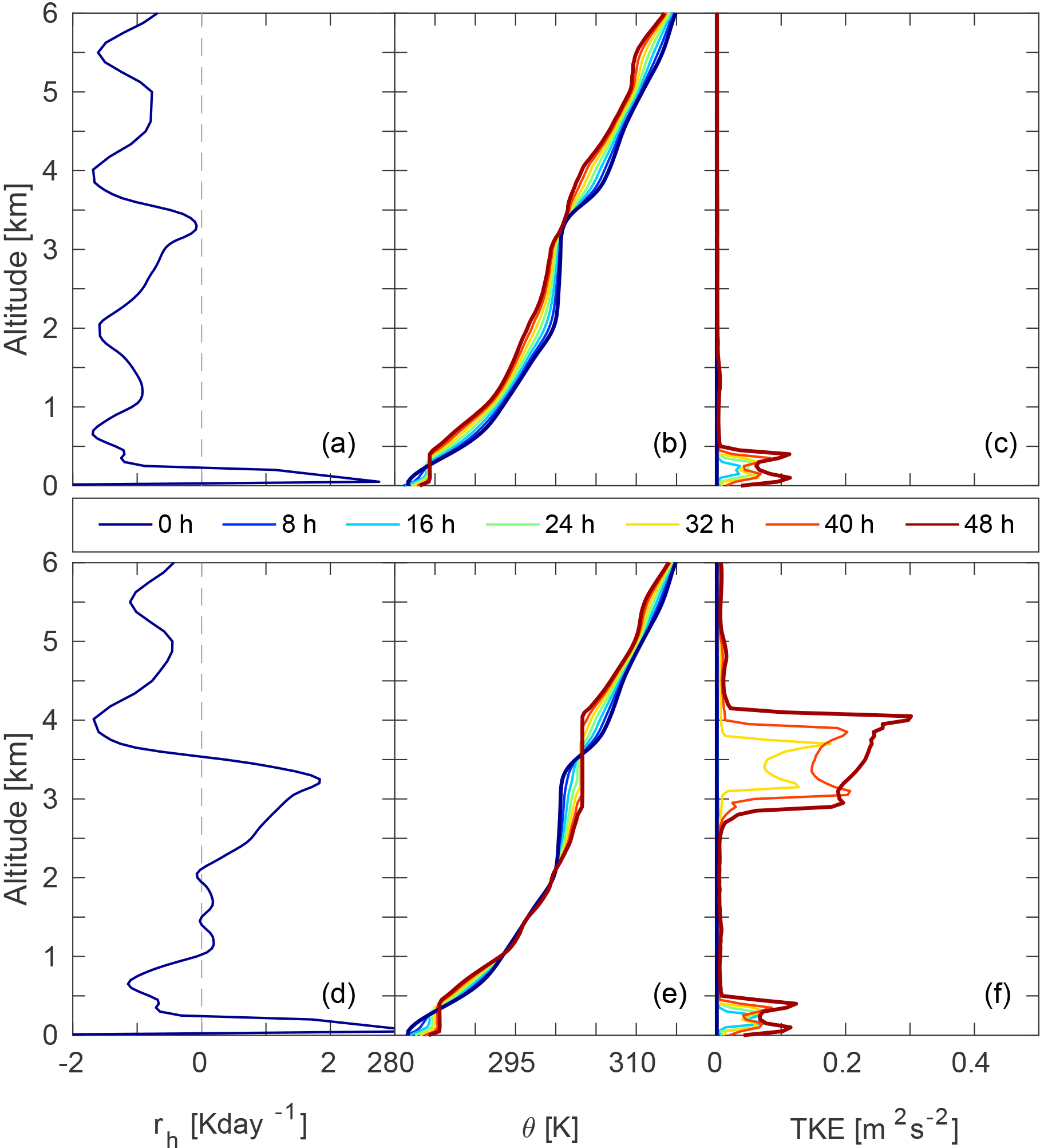
Figure 7 Vertical profiles of applied heating rate r_h (a, d), horizontally averaged potential temperature θ (b, e), turbulent kinetic energy TKE (c, f) for simulations of a clean case (a–c), and a polluted case with effects of aerosol load included (d–f). Simulation data are stored at 8 h intervals.

Outside the clearly turbulent regions, very little vertical mixing takes place, and the potential temperature is approximately given by

$$\begin{array}{}\text{(15)}& \mathit{\theta }=\mathit{\theta }(\mathrm{0},z)+r_{\mathrm{h}}\cdot t,\end{array}$$

where z symbolizes altitude and t time.

The obtained ILES results help us understand the potential effects of a BB plume on atmospheric dynamics on a local scale. Furthermore, the observed local production of turbulence and the associated vertical motion, may in turn affect factors such as cloud cover and the coupling between the surface layer and the plume layer, with potential effects on larger-scale dynamics. Further simulations, including water vapour and cloud condensate, are needed to study such effects in more detail.

4 Conclusions

This paper presented the investigation of a strong biomass-burning plume advection, which was observed during 9–11 July 2015 over the European Arctic. In this research study, we focused on the local perturbations in the radiation budget, as well as atmospheric dynamics for the Ny-Ålesund area on Spitsbergen. The discussed biomass-burning aerosol advection was one of the most spectacular in the last 25 years (Lund Myhre et al., 2007), with all aerosol optical properties typical for the summer conditions enhanced by a factor of more than 10. In particular, mean daily values of aerosol optical depth at 550 nm, precipitable water, and single-scattering albedo exceeded 0.2–0.7, 1.7–2.2 cm, and 0.93–0.97, respectively, according to in situ and photometer data at Ny-Ålesund. Here, we want to underline the most significant outcomes from our investigation:

• Simulations with the GEM-AQ model confirmed the source region (Alaskan tundra) and the arrival time at Ny-Ålesund of the biomass-burning plume, indicating a reasonable agreement in the extinction profile when compared to lidar measurements. The apparent underestimation of aerosol loading in the plume may be associated with rather coarse horizontal and vertical resolutions. Also, the large distance from the source region (approximately 4000 km) may have enhanced the uncertainties in the model output.

• Retrieved effective radius from in situ measurements of around 0.18 ± 0.02 µm, mean value of single-scattering albedo of 0.96, and an average asymmetry parameter exceeding 0.62 (all at ambient conditions) suggest moderate absorbing properties of the plume. Presented properties are in agreement with the results obtained by Nikonovas et al. (2015), who characterized a various set of smoke optical and microphysical properties retrieved from AERONET stations. Taking into account that BB variables are preferably placed in the lower part of the statistics in Nikonovas et al. (2015), we may conclude that during this prolonged transport, scavenging processes were more efficient.

• Lidar profiles indicate the existence of a biomass-burning plume at the level of 0–3.5 km, with a complicated structure of sublayers, limited by a number of (2–5) temperature inversions. A complex vertical variability is also visible in the relative humidity profile. The retrieved ω^a profiles vary from 0.92 to 0.97, enhancing with time. The highest values are associated with the bottom part of temperature inversions.

• The accuracy of modelled irradiances during the summer background conditions, represented by 09:00–14:00 9 July, is considered sufficient, with deviations from the measured quantities by 2 and 1 % for F_in and F_out, respectively. During the biomass-burning event (14:00 9 July–11:30 11 July) the differences increase to 10 and 5.8 % on average.

• We report mean values of modelled RF_surf, RF_atm, and RF_toa for the biomass-burning episode under study (14:00 9 July–11:30 11 July), at the levels of −78.9, −47.0, and 31.9 W m⁻². The values indicate cooling effects at the surface and the TOA, while RF_atm reveals relatively strong heating within the atmosphere. This might be translated up to 2 K day⁻¹ of the heating rate inside the smoke plume (0–3.5 km). Obtained values are consistent with results reported for the similar period, and likely the same solar zenith angles performed by Stone et al. (2008).

• An averaged RFE_surf at the smoke event is as high as −125.9 W m${}^{-\mathrm{2}}/{\mathit{\tau }}_{\mathrm{550}}$, indicating higher values in comparison with RFEs_surf obtained for wildfires from boreal regions (Markowicz et al., 2002, 2016b), while for other fire sources it is considerably lower by 12–32 % (García et al., 2012). The authors believe the main reason for different aerosol intensive properties is the distinct solar zenith angle and a high value of daily mean solar radiation at the TOA during the Arctic summer.

• The discrepancies between modelled RFs obtained for MODTRAN and fast Fu–Liou simulations oscillate around 15 %, with lower values usually attributed to the latter, excluding the atmospheric values. Considering different inputs and spatial resolution used for both simulations, the results are satisfactory.

• The mean bias of RFs associated with single-cell RF simulations in the vicinity of Kongsfjorden is estimated by the 3-D Monte Carlo model at the level of 2 W m⁻².

• ILES indicates that the main impact of the BB plume on the atmospheric dynamics is a gradual vertical expansion and positive displacement of the BB layer characterized by neutral stratification. The turbulent kinetic energy in the simulated BB layer is around 0.3 m² s⁻². In a clean simulation, without effects from the BB plume included, the flow remained nearly non-turbulent throughout the simulation period.

In this study we have shown that long-range transport of wildfire aerosols from Alaska to the European Arctic certainly has a significant impact on radiative properties. Furthermore, our results also indicate an impact on atmospheric dynamics. We believe that detailed studies on this topic are needed, especially considering the significant positive trend in mid-latitude fire frequency during the summer season over the last 25 years, and therefore possibly more frequent advection over the Arctic region (Young et al., 2017).