Ozone response to emission reductions in the southeastern United States

Ozone (O₃) formation in the southeastern US is studied in relation to nitrogen oxide (NO_x) emissions using long-term (1990s–2015) surface measurements of the Southeastern Aerosol Research and Characterization (SEARCH) network, U.S. Environmental Protection Agency (EPA) O₃ measurements, and EPA Clean Air Status and Trends Network (CASTNET) nitrate deposition data. Annual fourth-highest daily peak 8 h O₃ mixing ratios at EPA monitoring sites in Georgia, Alabama, and Mississippi exhibit statistically significant (p < 0.0001) linear correlations with annual NO_x emissions in those states between 1996 and 2015. The annual fourth-highest daily peak 8 h O₃ mixing ratios declined toward values of ∼ 45–50 ppbv and monthly O₃ maxima decreased at rates averaging ∼ 1–1.5 ppbv yr⁻¹. Mean annual total oxidized nitrogen (NO_y) mixing ratios at SEARCH sites declined in proportion to NO_x emission reductions. CASTNET data show declining wet and dry nitrate deposition since the late 1990s, with total (wet plus dry) nitrate deposition fluxes decreasing linearly in proportion to reductions of NO_x emissions by ∼ 60 % in Alabama and Georgia. Annual nitrate deposition rates at Georgia and Alabama CASTNET sites correspond to 30 % of Georgia emission rates and 36 % of Alabama emission rates, respectively. The fraction of NO_x emissions lost to deposition has not changed. SEARCH and CASTNET sites exhibit downward trends in mean annual nitric acid (HNO₃) concentrations. Observed relationships of O₃ to NO_z (NO_y–NO_x) support past model predictions of increases in cycling of NO and increasing responsiveness of O₃ to NO_x. The study data provide a long-term record that can be used to examine the accuracy of process relationships embedded in modeling efforts. Quantifying observed O₃ trends and relating them to reductions in ambient NO_y species concentrations offers key insights into processes of general relevance to air quality management and provides important information supporting strategies for reducing O₃ mixing ratios.

1 Introduction

Ozone (O₃) is a well known and important product of photochemical processes in the troposphere involving nitric oxide (NO), nitrogen dioxide (NO₂), and volatile organic compounds (VOCs). Ozone is of broad interest for its adverse effects on humans and ecosystems, as reflected by regulation through the US Clean Air Act (e.g., U.S. EPA, 2014, 2015a).

Regulatory actions address extreme O₃ mixing ratios: the US National Ambient Air Quality Standard (NAAQS), currently 70 ppbv, is applicable to the annual fourth-highest daily 8 h maxima averaged over 3-year periods (U.S. EPA, 2015b, c). By the early 1990s, US emission control efforts began to focus on nitrogen oxides (NO_x = NO + NO₂) in addition to VOCs (NRC, 1991). O₃ management has generally relied on precursor reduction requirements estimated from models that integrate descriptions of nonlinear chemical and atmospheric processes (e.g., Seigneur and Dennis, 2011), and guidance has also derived from so-called “observation-based” models linking O₃ and its precursors based on chemical reactions that are believed to drive ambient mixing ratios (e.g., NARSTO, 2000; Schere and Hidy, 2000).

Most of the work developing an observational basis for O₃-precursor chemistry derives from field campaigns, sometimes focusing on urban conditions. Short-term data are available from aircraft flights, for example, or summer field measurements made at a variety of locations. Such studies usually are limited to a month or two of intense sampling. One example in the southern US is the 1990 ROSE experiment at Kinterbish, a rural, forested state park in western Alabama (Frost et al., 1998). This summer study of rural O₃ at low anthropogenic VOC and low NO_x mixing ratios provided important insights into rural O₃ formation (Trainer et al., 2000). Other examples of short-term campaigns across the US and elsewhere are reviewed in Solomon et al. (2000). More recent field studies include New England in 2002 (e.g., Griffin et al., 2004; Kleinman et al., 2007), Texas in 2006 (e.g., Neuman et al., 2009), the mid-Atlantic region in 2011 (He et al., 2013), California in 2010 (Ryerson et al., 2013), Colorado in 2012 and 2014 (e.g., McDuffie et al., 2016), and the southeastern US in 2013 (e.g., Neuman et al., 2016; Warneke et al., 2016). These campaigns and accompanying analyses of O₃ production and accumulation typically address summer, which historically has the strongest photochemical activity. However, strong photochemical O₃ production can occur under special circumstances in winter (e.g., Schnell et al., 2009).

Accounting for an O₃ background is important. O₃ background is associated with biogenic influence, large-scale transport, or the potential influence of the upper atmosphere (e.g., stratospheric intrusions, especially during spring; Lin et al., 2012; Langford et al., 2015). The nature and magnitude of background O₃ remain an active area of research in the US and Europe (Naja et al., 2003; Solberg et al., 2005; Ordóñez et al., 2007; Cristofanelli and Bonasoni, 2009; Arif and Abdullah, 2011; Zhang et al., 2011; Wilson et al., 2012). Hidy and Blanchard (2015) discuss definitions of continental and regional background O₃. For this study, we adopt a definition of “background” that includes both the non-anthropogenic component and the southeastern regional component (Sect. 4.4.1).

Field studies have provided observational evidence of nonlinearity in O₃–NO_z relationships (e.g., Trainer et al., 1993, 1995; Kleinman et al., 1994; Hirsch et al., 1996; Frost et al., 1998; Kasibhatla et al., 1998; Nunnermacker et al., 1998; St. John et al., 1998; Sillman et al., 1998; Zaveri et al., 2003; Griffin et al., 2004; Travis et al., 2016). Long-term, post-1990s data are widely available for O₃ and NO₂ but detailed observations of total oxidized nitrogen (NO_y) and VOC, and especially their component species, are typically lacking (e.g., Hidy and Blanchard, 2015). One of the longest records of urban and suburban data, comprising a series of short-term campaigns as well as continuous measurements, is from southern California. This region exemplifies a photochemically active urban regime. An analysis of multi-decadal (since the 1960s) data by Pollack et al. (2013) reveals how changes in atmospheric chemical reactions have contributed to the observed reductions of O₃ in southern California since 1973. Long-term (more than one decade) measurements characterizing O₃ and NO_y relationships in both urban and rural conditions are less common.

The photochemical regime in the southeast represents humid subtropical conditions with urban emissions yielding elevated O₃ levels superimposed on a general regional background (Chameides and Cowling, 1995). The EPA O₃ and deposition data provide a regional basis for characterizing trends since the early 1980s (U.S. EPA, 2016a, b). In addition, the Southeastern Aerosol Research and Characterization (SEARCH) project (Hansen et al., 2003; Hidy et al., 2014) provides measurements that can be used to investigate changes in O₃ production resulting from changes in anthropogenic emissions in the southeastern US. The SEARCH network of eight sites began with the Southeastern Oxidant Study (SOS) (Chameides and Cowling, 1995; Meagher et al., 1998) rural locations, which were near (1) Centreville, AL, ∼ 85 km southwest of Birmingham; (2) at Yorkville, GA, ∼ 60 km northwest of Atlanta, GA; and (3) at Oak Grove, MS, ∼ 40 km southeast of Hattiesburg, MS, and 75 km north of Gulfport, MS, on private land within the confines of the De Soto National Forest (Hansen et al., 2003). Measurements of some gas-phase species began at these rural sites in 1992, thus providing a rural data record of over 20 years. Beginning in 1999, SEARCH added five sites in metropolitan Atlanta, GA; Birmingham, AL; Pensacola, FL; and Gulfport, MS.

Our goal for this study is to extend earlier analyses of the photochemical response of O₃ to precursors through 2014, emphasizing relationships between O₃ and NO_y. We first summarize relevant O₃ photochemistry to provide a context for the observational analysis. We then describe trends in emissions and ambient pollutant concentrations, and discuss O₃, NO_z, and HNO₃ observations at the SEARCH sites. The trends in O₃ mixing ratio, NO_x precursor emissions, and ambient nitrogen oxide mixing ratios offer important insight into future changes in O₃ and NO_y. Blanchard et al. (2014) previously explained the majority (66–80 %) of the day-to-day variations in daily peak 8 h average O₃ at SEARCH sites during March–October of 2002–2011 using meteorological variables coupled with ambient measurements of O₃ precursors (NO, NO₂; limited measurements of VOCs) and NO_x photochemical reaction products (NO_z) and a statistical model. The previous analyses are extended here for data through 2014 to help understand ongoing and potential future O₃ changes in relation to changes in ambient NO_z and HNO₃ mixing ratios in the southeastern US. Results are discussed in relation to modeling predictions by Reynolds et al. (2004) and others.

2 Ozone–nitrogen oxide chemistry

2.1 Key atmospheric reactions linking O₃ with NO_x

Net tropospheric O₃ accumulation occurs when sunlight acts on VOC and NO_x emissions and the O₃ production rate exceeds O₃ loss (Trainer et al., 2000). Tropospheric O₃ mixing ratios are affected by solar intensity, chemical formation and loss (e.g., deposition) rates of O₃, the rate of dispersion of O₃ and its precursors, meteorological factors, and vertical entrainment and transport of plumes. NO₂ forms rapidly by reaction of NO with O₃ and photolysis of NO₂ produces O₃, yielding steady-state mixing ratios of NO, NO₂, and O₃ in the absence of other species as expressed by the photostationary state, or Leighton relationship (Seinfeld, 1986).

In the troposphere, NO₂ also forms by reaction of NO with peroxy (HO₂) and alkyl peroxy (RO₂) free radical species, which derive in turn from the reaction of VOCs with hydroxyl (HO), HO₂, RO₂, and alkyl radicals (Seinfeld, 1986). Radical production from VOCs creates a pathway for conversion of NO to NO₂ that does not consume O₃ (Atkinson, 2000), which then leads to higher O₃ mixing ratios.

O₃ accumulation is typically associated with high solar radiation intensity and temperatures favoring atmospheric reactions, lower wind speeds, and high anthropogenic emission rates (NARSTO, 2000). O₃ accumulation requires NO mixing ratios exceeding approximately 10 to 30 pptv (Atkinson, 2000; Logan, 1985), along with the presence of HO₂ and RO₂ radicals that react with NO to form NO₂. The former conditions are normally met in urban air; NO_x mixing ratios are much lower under typical conditions in rural southeastern areas, but still well above 30 pptv (e.g., Hudman et al., 2007; Travis et al., 2016). Under these conditions, the O₃ photochemical production rate is proportional to the ambient NO multiplied by the sum of HO₂ and RO₂ radical mixing ratios, where the latter are weighted by their rates of reaction with NO (Trainer et al., 2000). Field studies show that observed rates of rural O₃ production are proportional to the rate of oxidation of NO_x. Where VOCs are present for radical production and NO_x is rate limiting (Trainer et al., 2000), regional O₃ production can be expressed in terms of the derivative d[O₃]∕d[NO_x], denoted as the O₃ production efficiency (OPE) (Liu et al., 1987). OPE is understood as the number of molecules of O₃ formed per molecule of NO_x oxidized and OPE increases as NO_x mixing ratios decrease (Liu et al., 1987; Trainer et al., 2000). OPE reflects the mean number of NO–NO₂ cycles occurring, in which each photolysis of one NO₂ molecule generates one O₃ molecule until that NO₂ molecule is oxidized to nitric acid (HNO₃) or to other species such as peroxyacetyl nitrate (PAN). NO_x reaction products, including HNO₃ and PAN, comprise NO_z. For chemical reactions, the quantity d[O₃]∕d[NO_z] is equivalent to d[O₃]∕d[NO_x], but with opposite sign, and has therefore been used to estimate OPE; limitations due to confounding influences of emissions, transport, and deposition are discussed in Sect. 4.3 and 4.4.

Empirically, the slope of a linear fit of afternoon O₃ (or O_x = O₃ + NO₂) versus NO_z has been used to estimate OPE (e.g., Trainer et al., 1993; Pollack et al., 2013). This estimate is subject to certain limitations because it does not explicitly account for (1) day-to-day variability in “old” (baseline or regional background) O₃ mixing ratios, (2) mixing of air masses having different emission histories, (3) rapid loss of HNO₃ (primarily through dry deposition, but also through gas-to-particle conversion) (Trainer et al., 2000), and (4) regeneration of NO₂ from PAN and certain other species. Because PAN regenerates NO₂, it can serve as a reservoir rather than a true NO₂ sink (Singh and Hanst, 1981; Singh, 1987). In contrast, HNO₃ largely terminates the cycling between NO and NO₂. Therefore, the relative yields of PAN and HNO₃ are of importance. Despite such limitations in using measurements to quantify OPE, data from field studies have been used since the 1990s to determine upper bounds for OPE and the results have continued to appear in the literature as an indicator of relevance to O₃ chemistry (e.g., Berkowitz et al., 2004; Neuman et al., 2009; Kim et al., 2016). Investigators caution that field measurements reveal the net of production and loss, which potentially overestimates actual OPE by factors of 3 to 6 due to rapid chemical and deposition losses of HNO₃ and other NO_z species (e.g., Trainer et al., 2000). Additional discussion is found in Sect. 4.4.

In southern California, changes in the relative proportions of NO_x-oxidation products have occurred and are thought to be instrumental in driving the rapid rates of O₃ decline in that area (Pollack et al., 2013). These results indicate that measurements of HNO₃ or PAN are needed to identify important changes in chemical pathways.

2.2 National O₃ response to emission reductions

Between 1980 and 2013, the national average of the annual fourth-highest peak daily 8 h O₃ mixing ratios, a metric relevant to the US O₃ NAAQS, declined by 33 % (U.S. EPA, 2015d) as national VOC and NO_x emissions decreased by 53 and 52 %, respectively (U.S. EPA, 2015e). Across the US and on multiple spatial scales from continental to urban, annual fourth-highest daily peak 8 h O₃ mixing ratios between 1980 and 2013 show a statistically significant (p < 0.05) linear fit to either annual average or to 98th percentile daily maximum hourly NO₂ mixing ratios; regression slopes are less than 1 : 1 and intercepts are in the range of 30 to 50 ppbv O₃ (Hidy and Blanchard, 2015). Proportionalities between O₃ and NO₂ that are less than 1 : 1 are expected, and the observed intercept terms are approximately consistent with typical O₃ mixing ratios of ∼ 20–50 ppbv observed at remote monitoring sites (Oltmans et al., 2008, 2013; U.S. EPA, 2012; Fiore et al., 2014; Lefohn et al., 2010, 2014; Cooper et al., 2012, 2014).

Although nonlinearity of O₃ production and accumulation with respect to ambient VOC and NO_x is well established (Lin et al., 1988), a tendency toward linearity is expected at sufficiently low NO_x mixing ratios. As an example, the O₃ photochemical production rate during June 1990 at Kinterbish, AL, was approximately linear over a range of ambient NO_x from 0.1 to 2 ppbv (Trainer et al., 2000). Observed O₃ extrema can also exhibit an apparent linear or near-linear response to ambient NO_x mixing ratios if the extrema consistently fall within the lower-right quadrant (NO_x-sensitive regime) of an O₃–VOC–NO_x diagram, a concise graphical representation first established empirically from southern California data and later generated using the Empirical Kinetic Modeling Approach (EKMA) (illustrated in Hidy and Blanchard, 2015). The O₃–VOC–NO_x diagram has been adopted by many investigators for displaying the output of box models (e.g., Fujita et al., 2003, 2015) and grid-based photochemical models (e.g., Reynolds et al., 2003, 2004).

Southern California historically has exhibited the highest peak O₃ mixing ratios in the US since the 1960s. Because of high ambient O₃ and precursor mixing ratios there and the complexity of the relationships of O₃ with NO_x and VOC, some investigators have described southern California O₃ and precursor trends in terms of percentage changes. For example, Pollack et al. (2013) report that peak 8 h O₃ mixing ratios in southern California declined exponentially over time at a rate of 2.8 % per year between 1973 and 2010, thus decreasing O₃ levels by approximately a factor of 3. This rate of O₃ decline exceeds rates occurring in other metropolitan areas (Hidy and Blanchard, 2015). O₃ extrema in southern California decreased along with declining mixing ratios of ambient VOCs and NO_x (7.3 % yr⁻¹ and 2.6 % yr⁻¹, respectively, 1960–2010) and declining ratios of VOC ∕ NO_x (4.8 % yr⁻¹) (Pollack et al., 2013). The rates of atmospheric oxidation of NO_x increased over time and changes in NO_x oxidation reactions increasingly favored production of HNO₃, a NO_x reaction product associated with radical termination and quenching of the O₃ formation cycle (Pollack et al., 2013). To our knowledge, changes in the relative proportions of atmospheric reaction products accounting for rapid rates of O₃ reduction have not been reported for locations other than southern California.

3 Methods

3.1 Emissions and ambient air quality measurements

Air quality monitoring data were obtained from the EPA Air Quality System (AQS) data archives for all sites in Georgia, Alabama, and Mississippi (U.S. EPA, 2016a). Daily measurement values (i.e., peak daily 8 h O₃ mixing ratio) as well as annual summary statistics (e.g., maxima, annual averages) were acquired. We obtained deposition data from the two EPA Clean Air Status and Trends Network (CASTNET) monitoring sites located within the study region: Sand Mountain, AL (125 km east-northeast of the SEARCH site at Centreville), and Georgia Station, GA (102 km SE of the SEARCH site at Yorkville) (U.S. EPA, 2016b).

Annual, state-level emission trends data were obtained from the U.S. EPA (2016c, d), Xing et al. (2013), and Hidy et al. (2014). The comparability of inventories is discussed in the Supplement (Fig. S1). Because the EPA trend inventory utilized different methods for estimating mobile-source emissions prior to 2002 compared with 2002 and later years, we combined EPA trend estimates for 2002–2016 with the 1996–2001 emission estimates of Hidy et al. (2014), which are consistent with more recent EPA methods (see Supplement).

Hourly measurements of gases (NO, NO₂, NO_y, HNO₃, and O₃) were obtained from SEARCH public archives (ARA, 2017). All parameters measured at the sites are calibrated and audited to conventional reference standards, as described in ARA (2015). Network operations, sampling, and measurement methods are documented in Hansen et al. (2003, 2006); see also Table S1 in the Supplement. The network consisted of eight extensively instrumented monitoring sites located in the southeastern US along the Gulf of Mexico and inland (Fig. S2): Pensacola, Florida (PNS), and Gulfport, Mississippi (GFP), urban coastal sites (∼ 5 and 1.5 km from the shoreline, respectively); Pensacola – outlying (aircraft) landing field (OLF) and Oak Grove, Mississippi (OAK), non-urban coastal sites near the Gulf (∼ 20 and 80 km inland, respectively); Atlanta, Georgia – Jefferson Street (JST) and North Birmingham, Alabama (BHM), urban inland sites; and Yorkville, Georgia (YRK), and Centreville, Alabama (CTR), non-urban inland sites. PNS, OAK, and GFP were closed at the end of 2009, 2010, and 2012, respectively. SEARCH site locations are described in detail, including discussion of possible emission influences, in Hansen et al. (2003) and Hidy et al. (2014). SEARCH VOC data are available for JST as daily data from 1999 through 2008, and U.S. EPA VOC measurements are available for YRK as summer hourly data and as 24 h samples collected every sixth day throughout the year (Blanchard et al., 2010a). EPA VOC samples are also available for three other sites in the Atlanta area; only one of these additional sites reported data through 2014.

SEARCH meteorological parameters and gases are sampled at a height of 10 m, characteristic of lower-tropospheric mixing ratios near the surface (Hansen et al., 2003, 2006; Edgerton et al., 2007; Saylor et al., 2010). Gas and meteorological measurements commenced in 1992 at the rural sites of CTR, OAK, and YRK. The measurements at rural SEARCH sites included O₃, NO, and NO_y beginning in 1992, and NO₂ and HNO₃ measurements began in 1996. Consistent measurement methods have been utilized for all gases except NO₂. NO₂ measurements commenced network-wide in 2002, and three NO₂ measurement methods have been employed during the network operations (Table S3). All three methods are NO₂-specific, differing primarily in the light source used for photolysis of NO₂. The NO₂ data exhibit consistency with NO and NO_y measurements but with some variations occurring during specific years (e.g., 2001 and 2002, Fig. S3). Because changes in NO₂ measurement methods could affect the computed NO_z (NO_y–NO–NO₂), we repeat some data analyses using HNO₃ in place of NO_z. As noted, HNO₃ data also provide useful insight into NO₂ termination reactions. HNO₃ measurements are the difference between NO_y and denuded NO_y (Table S1; Hansen et al., 2006). The SEARCH measurements of NO_y were designed to capture particulate nitrate and organic nitrates, as well as NO, NO₂, HNO₃, and other oxidized nitrogen species. The NO_y sampler derives from the instrument identified in Williams et al. (1998) as Environmental Science and Engineering (ESE), which was one of five instruments for which measurements of NO_y reproduced the sum of separately measured NO_y species. Additional testing in 2013 showed that SEARCH NO_y measurements agreed with the sum of measured mixing ratios of NO, NO₂, HNO₃, particulate nitrate, alkyl nitrates, and peroxy–alkyl nitrates (Hidy et al., 2014).

Trace gas calibrations were done daily for O₃ and every third day for other gases. Reported detection limits (Table S1) are 0.05–0.1 ppbv for oxidized nitrogen species and 1 ppbv for O₃ (Hansen et al., 2003, 2006). NO₂ measurement uncertainties are estimated as ∼ 30 % prior to 2002 and ∼ 10 % after 2002 (Hansen et al., 2006). Measurement uncertainties are estimated to be 10 % or less for other oxidized nitrogen species and 5 % or less for ozone (2σ in all cases). Propagation of errors indicates corresponding 2σ measurement uncertainties averaging 0.5 ppbv for mid-afternoon NO_z (< 0.1 ppbv for NO_z < 1 ppbv) and 0.16 for the ratio NO_z ∕ NO_y.

3.2 Data analysis

Multiple methods were employed to characterize the variability of ambient O₃ and NO_y mixing ratios. Analyses of seasonal variability used data from all months of each year. Diurnal hourly average mixing ratios were computed by year to characterize patterns of temporal change and to identify hours associated with O₃ maxima. Observed slopes of regressions of O₃ versus NO_z were computed as previously done in measurement studies using afternoon O₃ and NO_z data (Trainer et al., 1993, 1995; Kleinman et al., 1994; Hirsch et al., 1996; Kasibhatla et al., 1998; Nunnermacker et al., 1998; St. John et al., 1998; Sillman et al., 1998; Zaveri et al., 2003; Griffin et al., 2004; Travis et al., 2016). Because past studies have examined O₃ formation in photochemically aged air (i.e., at locations distant from fresh emissions, where atmospheric reactions have acted on emissions from earlier times) during summers (e.g., Trainer et al., 1993), our analyses focus on the months of June and July to select weeks nearest maximum solar radiation (∼ −20, +40 days). Additional analyses were carried out for other months to facilitate comparisons across seasons. As for earlier studies, the calculations are based on afternoon times, using hourly values starting at 14:00 local standard time to represent the daily peak O₃ after morning production and before mixing ratios decline with decreasing photochemical reaction in later afternoon. In addition to characterizing O₃ ∕ NO_z and its change with time, corresponding supporting analyses are presented for O₃ ∕ HNO₃. As a supplemental analysis, rates of maximum diurnal increase of O₃ and HNO₃ during late morning and early afternoon were computed for comparison of ΔO₃ with ΔHNO₃.

4 Results and discussion

4.1 Trends

Hidy et al. (2014) report a 63 % reduction of NO_x emissions in the southeastern US between 1996 and 2014. The largest NO_x emission changes in the southeast occurred between 2007 and 2009 due to reductions of emissions from electric generating units (EGUs) and from diesel engine vehicles, and they were accompanied by more gradual year-to-year reductions of gasoline-engine mobile-source NO_x emissions (de Gouw et al., 2014; Hidy et al., 2014). NO_x emission reductions led to approximately proportional responses of mean ambient NO_y and NO_z mixing ratios at SEARCH sites (Hidy et al., 2014).

The EPA CASTNET data show wet and dry nitrate deposition since the late 1990s declining at rates of ∼ 5 % per year (−0.045 ± 0.005 and −0.056 ± 0.005 yr⁻¹), nearly identical to NO_x emission changes of −0.046 ± 0.001 and −0.051 ± 0.003 yr⁻¹ (Fig. 1). Total (wet plus dry) nitrate deposition fluxes decreased linearly in proportion to reductions of NO_x emissions in Alabama and Georgia (Fig. 1). Linear regression slopes indicate that the annual nitrate deposition fluxes at the Georgia and Alabama CASTNET sites correspond to 30 % of Georgia emissions and 36 % of Alabama emissions on an annual and statewide basis (Fig. 1). Emissions are not spatially homogeneous and deposition losses likely vary with distance from emission sources. The two sites are situated differently in relation to metropolitan areas, possibly affecting deposition fluxes; Sand Mountain (SND) is northeast of Birmingham and Georgia Station (GAS) is south of Atlanta. The linearity and statistical significance of the regressions indicate that the fraction of NO_x emissions lost to deposition has not changed over time (ratios of annual deposition to state emissions varied without trend from 0.23–0.34 at GAS and 0.30–0.45 at SND). Mean annual SEARCH NO_y mixing ratios at rural CTR and YRK declined at ∼ 5–7 % yr⁻¹ (Fig. S4). SEARCH and EPA CASTNET sites exhibit downward trends in mean annual HNO₃ concentrations of ∼ 9–11 and ∼ 6–7 % yr⁻¹, respectively (Fig. S4). Ambient NO_y and HNO₃ trends are not statistically different from state-level NO_x emission trends.

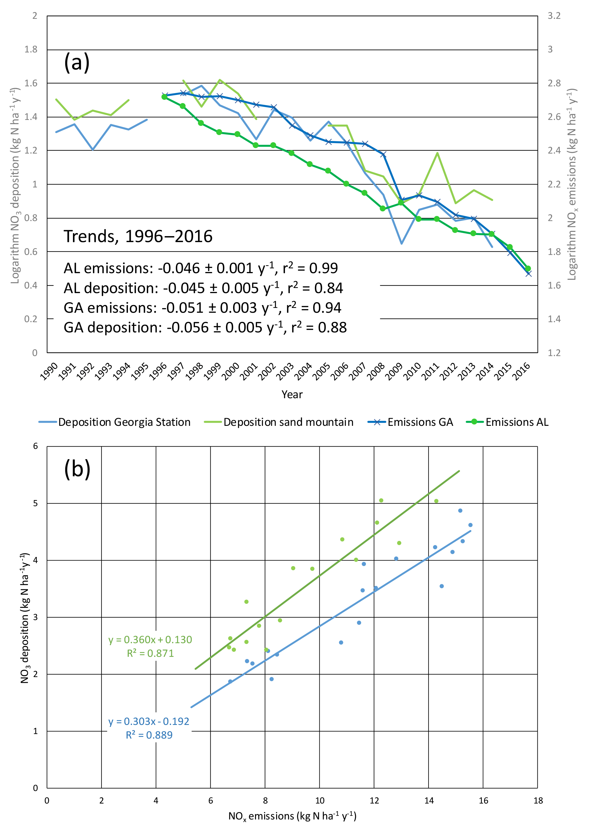
Figure 1 Comparison of nitrate deposition (wet plus dry) to NO_x emission densities in Georgia and Alabama as (a) temporal trends and (b) regression of deposition against emissions (with same color coding in both panels). Nitrate deposition and NO_x emission densities are expressed as kg ha⁻¹ yr⁻¹. NO_x emissions are from all source sectors (see Supplement). Panel (a) shows natural logarithms vs. year and indicates that emissions and deposition trended downward at the same rates. Panel (b) slopes are statistically significant (p < 0.0001) and intercepts are not (p > 0.1).

Annual fourth-highest daily peak 8 h O₃ mixing ratios at compliance monitoring sites in Georgia, Alabama, and Mississippi exhibit statistically significant (p < 0.0001) linear correlations with annual NO_x emissions in those states between 1996 and 2015 (Fig. 2), qualitatively consistent with past work indicating that high O₃ would respond to reductions of NO_x emissions (Chameides and Cowling, 1995; Jacob et al., 1995; Kasibhatla et al., 1998). Intersite differences in the annual fourth-highest daily peak 8 h O₃ mixing ratios have decreased (Fig. 2), consistent with an analysis of data from a larger number of US and European locations (Paoletti et al., 2014). The annual fourth-highest daily peak 8 h O₃ mixing ratios are declining toward nonzero values, as indicated by the statistically significant (p < 0.0001) intercepts of ∼ 45–50 ppbv (Fig. 2). SEARCH data are used to characterize the southeastern O₃ response to emission changes in greater detail. Between 1999 and 2014, the highest peak daily 8 h O₃ mixing ratios occurring each month (monthly O₃ maxima) declined at all SEARCH sites at statistically significant (p < 0.01) rates averaging ∼ 1–1.5 ppbv yr⁻¹ (Fig. 3). These declines are comparable to the trend in the 95th percentile summer peak daily 8 h O₃ mixing ratios in the southeastern US of ∼ −0.8 to −1.8 ppbv yr⁻¹ reported by Lin et al. (2017), with downward trends occurring in other seasons as well. The observed SEARCH O₃ trends are also consistent with other analyses of North American observations (e.g., Chan, 2009; Lefohn et al., 2010; Paoletti, 2014; Simon et al., 2015) and with the trends occurring at EPA monitors in the southeast (Fig. 2). Both EPA (Fig. 2) and SEARCH (Fig. 3) data suggest that O₃ mixing ratios increased during the 1990s, then began declining. This result is consistent with modeling by Reynolds et al. (2004), which predicted an initially slow response of Atlanta-area O₃ to emission reductions between 1996 and 2000, followed by increasing sensitivity to reductions of NO_x emissions. The observed O₃ decreases exceed those predicted by Reynolds et al. (2004) because actual NO_x emission reductions (∼ 60 % between 1996 and 2014) exceeded the projected emission reductions (∼ 40 % by 2010 and ∼ 55 % by 2020) that were anticipated based on known and anticipated emission control rules at the time of the modeling study. The SEARCH trends are compared with emission changes in the southeast and with emission and O₃ trends in southern California, in Table S2.

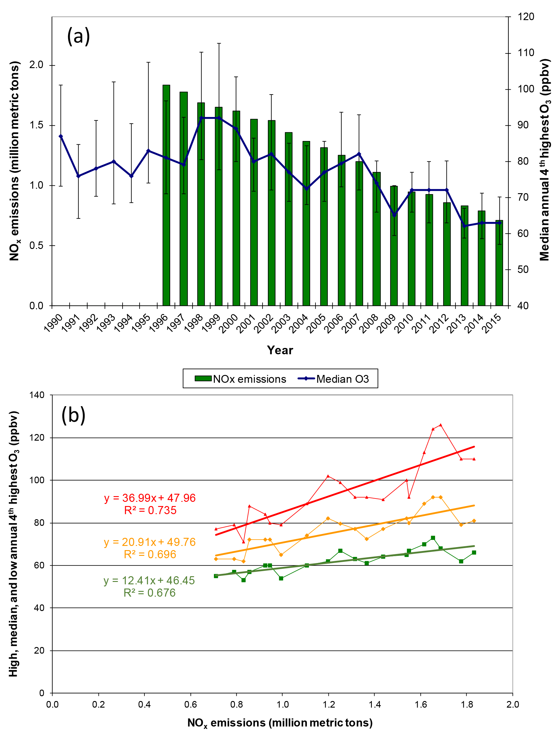
Figure 2 Comparison of annual fourth-highest daily peak 8 h O₃ to NO_x emissions in Georgia and Alabama (a) trends (±90th and 10th percentile sites) and (b) regressions (high = 90th percentile site, median, and low = 10th percentile site annual fourth-highest daily peak 8 h O₃). NO_x emissions are from all source sectors (see Supplement). O₃ data include all EPA AQS monitors in Georgia and Alabama for each year having at least 75 % data completeness (mean = 55 monitors, low of 32–36 in 1990–1993). Slopes and intercepts are statistically significant (p < 0.0001).

More complete understanding of regional O₃ trends requires consideration of both regional emission changes and possible changes in background O₃. Multiple definitions of the term “background O₃” may be found in the literature, including global background, continental background, non-anthropogenic background, and regional background, among others. For the O₃ trends shown in Figs. 2 and 3, the most relevant consideration is the amount of O₃ transported into the study domain across upwind boundaries (denoted here as regional background or transported O₃). The percentage reductions of O₃ are larger if transported O₃ can be estimated and subtracted from observed O₃ mixing ratios, and this adjustment potentially provides a better assessment of the effects of regional emission reductions on the fraction of O₃ that is manageable by means of local and regional emission control measures. For example, Parrish et al. (2017a) report that the O₃ enhancement above background in southern California decreased by 4.5 % yr⁻¹, which is larger than the unadjusted O₃ decline of 2.8 % yr⁻¹ given by Pollack et al. (2013). Similarly, rates of decline in southeastern US O₃ are larger if regional background O₃ is considered (Table S2).

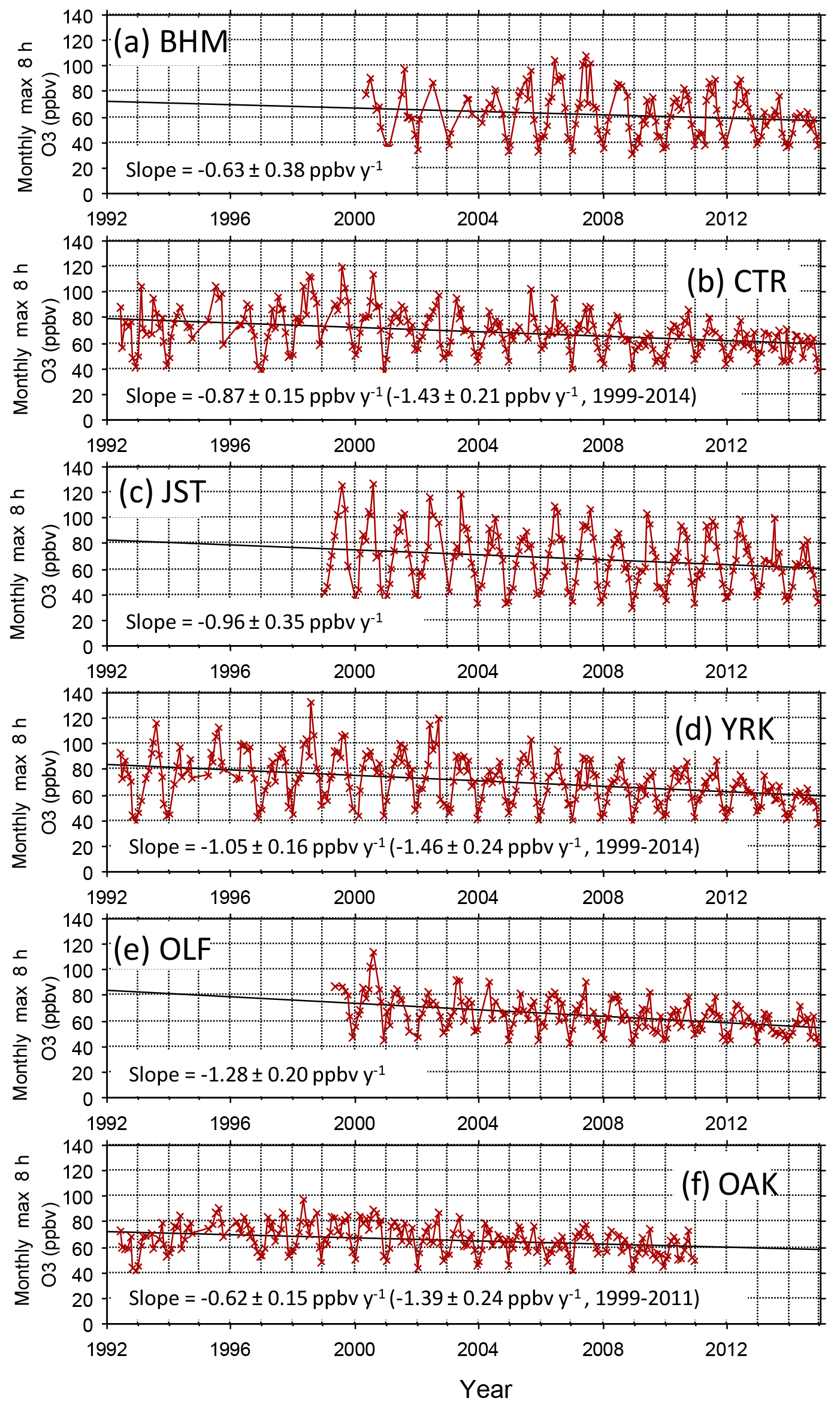
Figure 3 Monthly maxima of daily peak 8 h average O₃ mixing ratios. All monthly maxima are determined from 24 or more days with 18 or more sampling hours per day. PNS and GFP (not shown) exhibit trends of −1.64 ± 0.45 and −0.60 ± 0.32 ppbv yr⁻¹, respectively. Trends are statistically significant (p < 0.01) at CTR, JST, OAK, OLF, PNS, and YRK.

Figure 4 Monthly means of daily peak 8 h average O₃ mixing ratios. All monthly means are determined from 24 or more days with 18 or more sampling hours per day. Standard errors of the means average 2 (range 0.8–5) ppbv.

Defining and estimating regional background (or transported) O₃ are each challenging. We interpret the intercepts in Fig. 2 as indicators of mean O₃ levels that would occur on days with weather conducive to high O₃ in the absence of NO_x emissions from AL and GA sources, i.e., as estimators of O₃ transported into the region from outside the study domain (as discussed subsequently, multi-day carryover of local and regional emissions during stagnation events could also affect intercepts and slopes). Days with weather that is not conducive to high O₃ likely have different levels of transported O₃. The statistically significant slopes in Fig. 2 indicate O₃ enhancements that are attributable to AL–GA emissions, except as noted next, and a comparison of the O₃ decline to intercept-corrected O₃ would then reveal the proportionality between AL–GA emissions and AL–GA O₃ enhancements over O₃ originating outside the study domain (i.e., in excess of regional background O₃). Although the ∼ 30–35 % O₃ declines are less than proportional to the ∼ 60 % decrease in NO_x emissions, the decline in the median O₃ is ∼ 60 % if the 50 ppbv intercept shown in Fig. 2 is subtracted from the O₃ mixing ratios.

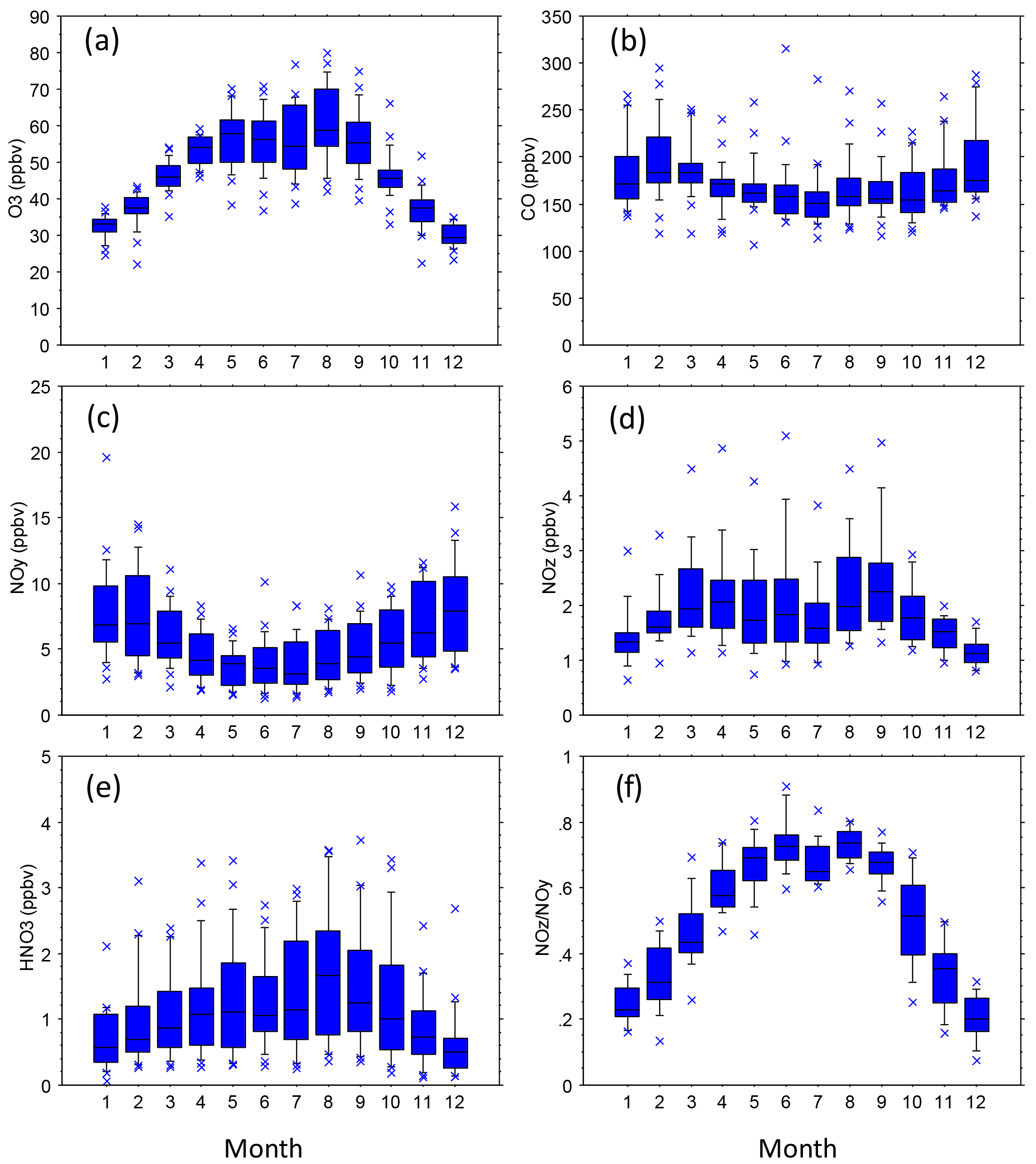
Figure 5 Statistical distributions of mean monthly species mixing ratios (all SEARCH sites, 1992–2014). Distributions indicate the 10th, 25th, 50th, 75th, and 90th percentiles of the monthly averages.

If the amount of O₃ that has been transported from upwind regions has been changing over time, e.g., declining as NO_x emissions and ambient O₃ decline in adjacent regions, the slopes shown in Fig. 2 would reflect changes in both the O₃ that originated upwind and in the O₃ enhancements attributable to AL–GA emissions, confounding attribution. Related studies do not provide consistent evidence for a trend, either upward or downward, in regional background O₃ in the southeastern US. For example, baseline O₃ concentrations in air flowing into Texas from the Gulf of Mexico during May through October did not change significantly between 1998 and 2012 (Berlin et al., 2013). Mean regional background O₃ mixing ratios were 48 to 59 ppbv in the Houston, TX, area on days with O₃ levels exceeding the NAAQS, which includes O₃ contributions from transport to the area from other regions of the US (Berlin et al., 2013). Observed trends in the 5th percentile O₃ have previously been used as indicators of changes in either regional or continental background O₃ (e.g., Wilson et al., 2012). The 5th percentile peak daily 8 h O₃ mixing ratios decreased during summer at rural sites throughout the southeastern US between 1988 and 2014 (Lin et al., 2017). By this measure, regional background O₃ levels did not increase in the southeastern US during our study period.

Large-scale transport affecting O₃ in the boundary layer and at the surface is a function of altitude. For example, during June 2013, anthropogenic emissions and long-range transport (long-range tropospheric + stratospheric) O₃ each accounted for about 40 % (15–20 ppbv each) of model-predicted O₃ below 1 km altitude at Huntsville, AL, while long-range transport accounted for ∼ 80 % of model-predicted O₃ above 4 km altitude (Johnson et al., 2016). This variation of source contributions with altitude provides an opportunity to differentiate between emission-related and transport-related trends derived from vertical soundings of upper-air O₃ mixing ratios. Using ozonesondes that are generally launched on a weekly schedule, vertical O₃ mixing ratio profiles have been determined by the University of Alabama in Huntsville, Alabama, since 1999 (Newchurch et al., 2003; Johnson et al., 2016; University of Alabama Huntsville, 2017; NOAA, 2017). We obtained these ozonesonde data (n=940 days) and identified the following statistically significant trends in the lower layers that are relatively more influenced by local and regional emissions according to Johnson et al. (2016): −0.25 ± 0.11 ppbv yr⁻¹ (p < 0.05) in daily measurements at 0.5 km, −0.40 ± 0.10 ppbv yr⁻¹ (p < 0.0001) at 1 km (daily), −0.42 ± 0.09 ppbv yr⁻¹ (p < 0.0001) at 2 km (daily), and −0.57 ± 0.13 ppbv yr⁻¹ in monthly averages of O₃ measurements made throughout the interval 1–2 km (p < 0.001). At higher altitudes where Johnson et al. (2016) predicted that long-range transport is the dominant source of O₃, no trends occurred: 0.06 ± 0.08 ppbv yr⁻¹ (p > 0.1) at 4 km (daily) and 0.09 ± 0.19 ppbv yr⁻¹ (p > 0.1) at 8 km (daily).

Global background is one component of regional background and trends in global background are expected to contribute to trends in regional background. Lin et al. (2017) show that rising NO_x emissions in Asia have increased modeled North American background O₃ levels (based on model simulations with zero North American emissions) by ∼ 0.2 ppbv yr⁻¹ in the southeastern US in summer, which is a small effect even when accumulated over 20 years in comparison with the ∼ 25 ppbv reduction in the median annual fourth-highest peak daily 8 h O₃ shown in Fig. 2. Multiple studies have demonstrated increasing trends in global background O₃ mixing ratios (Ordóñez et al., 2007; Oltmans et al., 2008; Arif and Abdullah, 2011; Wilson et al., 2012). Parrish et al. (2017a) report that the highest O₃ design values (the 3-year running mean of the annual fourth-highest peak daily 8 h O₃ mixing ratio) in southern California are converging toward a limit of 62.0 ± 1.9 ppb, which they identify as the O₃ design values that would result from US background O₃ concentrations. Parrish et al. (2017b) report decreasing O₃ transported across the Pacific into the western US after 2000. As noted, regional background O₃ in the southeastern US does not appear to be trending either upward or downward, even though trends in background O₃ have been established in other areas or globally.

In the southeastern US, the simple conceptual model of O₃ transported into a study region across upwind boundaries is incomplete. High O₃ typically occurs during multi-day stagnation episodes, which are associated with the presence of high barometric pressure over the domain and limited transport (Blanchard et al., 2013). Transport distances determined from 24 h back-trajectory computations are less than 300 km for the highest decile O₃ (Blanchard et al., 2013). Mean 24 h transport distances are less than 350 km during June and less than 380 km during July (Blanchard et al., 2014). These distances are approximately equivalent to distances from Birmingham to Mobile, AL, or from Atlanta to Savannah, GA. Local and regional emissions can accumulate over multiple days and potentially could contribute to observed O₃ concentrations (e.g., aloft) that are considered as regional background. In contrast to emissions originating upwind, carryover from emission sources within the study domain is a manageable component of efforts to reduce O₃.

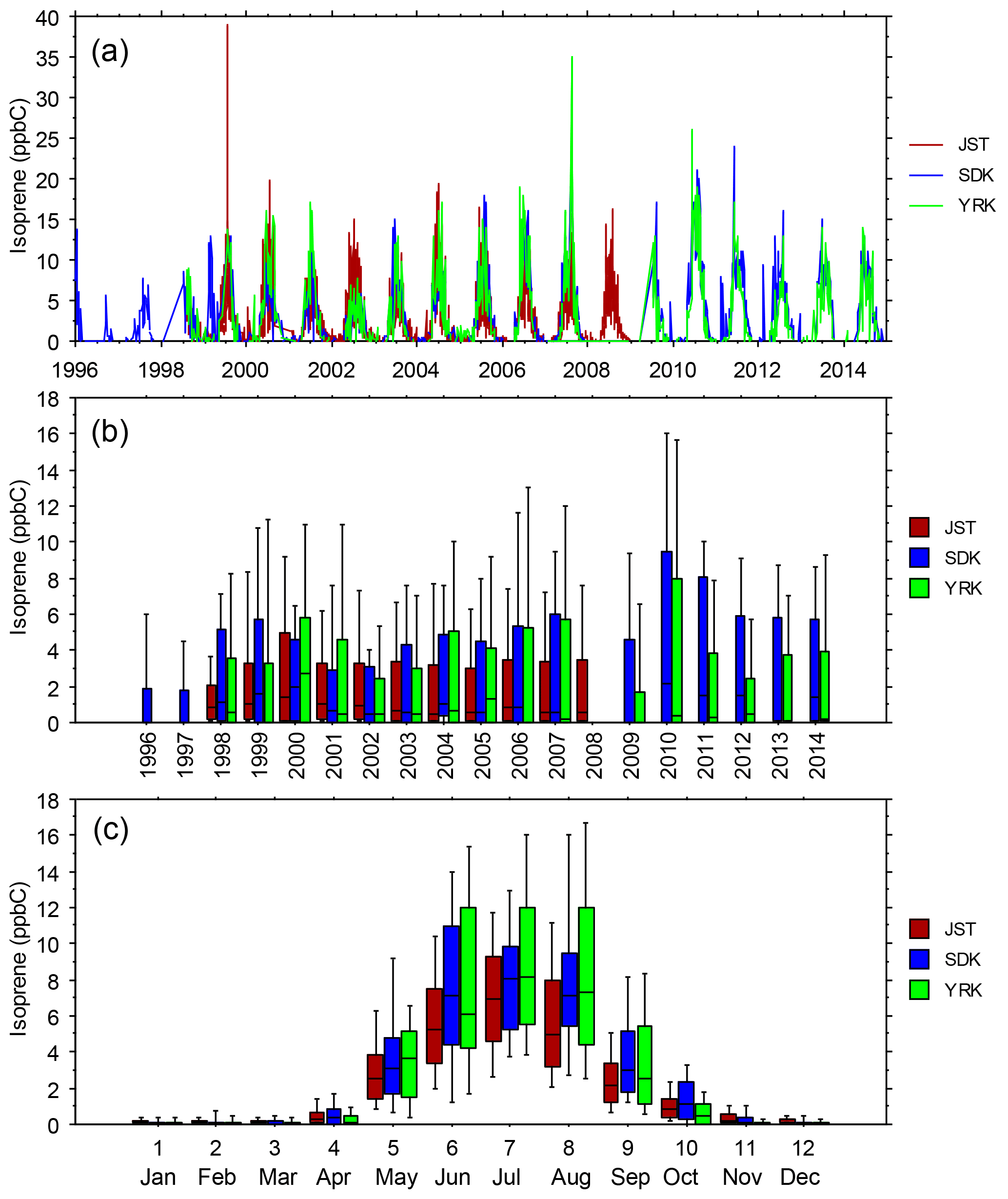
Figure 6 (a) Daily-average isoprene mixing ratios vs. date, (b) statistical distributions of daily-average isoprene mixing ratios vs. year, and (c) statistical distributions of daily-average isoprene mixing ratios vs. month. Samples were obtained every day at JST and once every 6 days at YRK and SDK (Blanchard et al., 2010a). Distributions indicate the 10th, 25th, 50th, 75th, and 90th percentiles.

4.2 Seasonal variations of O₃, NO_y, NO_z, HNO₃, and VOCs

The seasonal oscillations of monthly O₃ maxima in the southeast are coupled to local or regional meteorology, solar radiation, and emissions (e.g., Blanchard et al., 2013, 2014; Hidy et al., 2014). Variations of daily maximum temperature and midday relative humidity (RH) are associated with variations of daily peak 8 h O₃ mixing ratios by ∼ ±30 % from mean peak 8 h O₃ mixing ratios, after also accounting for variations of other meteorological factors (Blanchard et al., 2014). Air mass back trajectories originating from the south (∼ 150 to 200^∘) exhibit peak 8 h O₃ that is ∼ 5–10 % lower than average; daily peak O₃ decreases as 24 h back-trajectory distances increase from zero to ∼ 600 km, consistent with association of higher O₃ concentrations with air mass stagnation rather than transport (Blanchard et al., 2013, 2014). At SEARCH sites, the monthly O₃ maxima (highest daily peak 8 h O₃ each month) and mean daily peak 8 h O₃ mixing ratios typically occurred in summer months, especially inland, and declined more than other monthly maxima (Figs. 3 and 4). Summer means were not always higher than spring averages, especially at rural and coastal sites and during more recent years (Fig. 4). Roughly constant winter monthly peak 8 h maxima of ∼ 40 ppbv occurred throughout the period of record (Fig. 3). The seasonal variability of the highest peak daily 8 h O₃ therefore declined over time (see also Table S3). Similar results were found for monthly means of hourly measurements, discussed in Sect. 4.3 on diurnal variations. Other recent studies have reported decreasing seasonal variability of O₃ across the US using data from large numbers of monitoring sites (Chan, 2009; Chan and Vet, 2010; Cooper et al., 2012; Paoletti et al., 2014; Simon et al., 2015). Declines in seasonal variability are thought to result from changing rates of O₃ formation as precursor emissions have declined or from increasing influence of intercontinental background O₃, not from changes in seasonal variations of temperature and other meteorological factors (Chan, 2009; Cooper et al., 2012; Simon et al., 2015).

Figure 7 Average O₃ mixing ratios vs. hour, by year. Each data point is the mean of all hourly measurements during June through August. Sites at PNS and GFP (not shown) exhibit similar diurnal profiles and trends (sampling at those sites ended after 2009 and 2012, respectively). Standard errors of the means are 0.3–4 ppbv (∼ 2 % of mean O₃ mixing ratios).

The SEARCH data indicate that seasonal variations occur in ambient O₃, NO_y, NO_z, HNO₃, and the ratio of NO_z ∕ NO_y (Fig. 5). Seasonal variations of temperature and other meteorological factors are known to cause seasonal variations of O₃ and NO_y species concentrations. The monthly average NO_z and HNO₃ mixing ratios indicate that active photochemical processing of NO_x occurs during well over half the year in the warm climate of the southeastern US. The effects of VOC species on O₃ formation depend on both their ambient concentrations and their reactivities. To describe VOC variations at sites with long-term VOC measurements, we use isoprene data as an indicator of biogenic VOCs and toluene as an indicator of anthropogenic VOCs (nominally emitted as a gasoline vapor). The importance of isoprene emissions for O₃ production in the southeastern US is well established (e.g., Chameides et al., 1988; Chameides and Cowling, 1995; Frost et al., 1998; Starn et al., 1998; Wiedinmyer et al., 2006; Zhang et al., 2014; Lin et al., 2017). We also consider other reactive VOC species of interest, including α-pinene (biogenic) as well as ethylene and xylenes (anthropogenic). Summer (June–August) months exhibit elevated ambient mixing ratios of rural and urban isoprene, typically about 5–10 ppbC, that are 1 to 2 orders of magnitude greater than those occurring between October and April (Fig. 6). Transitions between low and high ambient isoprene mixing ratios occur in mid-May and mid-September in northern Georgia (Fig. 6). Annual mean isoprene mixing ratios were relatively constant, ∼ 2.5–3 ppbC, between 1998 and 2014. Biogenic VOCs, primarily isoprene, represent ∼ 20 % of the VOC reactivity at JST, ∼ 30 % at South DeKalb (SDK, located in metropolitan Atlanta ∼ 16 km southeast of JST), and ∼ 50 % at YRK, averaged over all samples collected between 1999 and 2007 (Blanchard et al., 2010a). Through precursor interactions, seasonal variations in isoprene mixing ratios are expected to affect seasonal variations in O₃ mixing ratios and production rates.

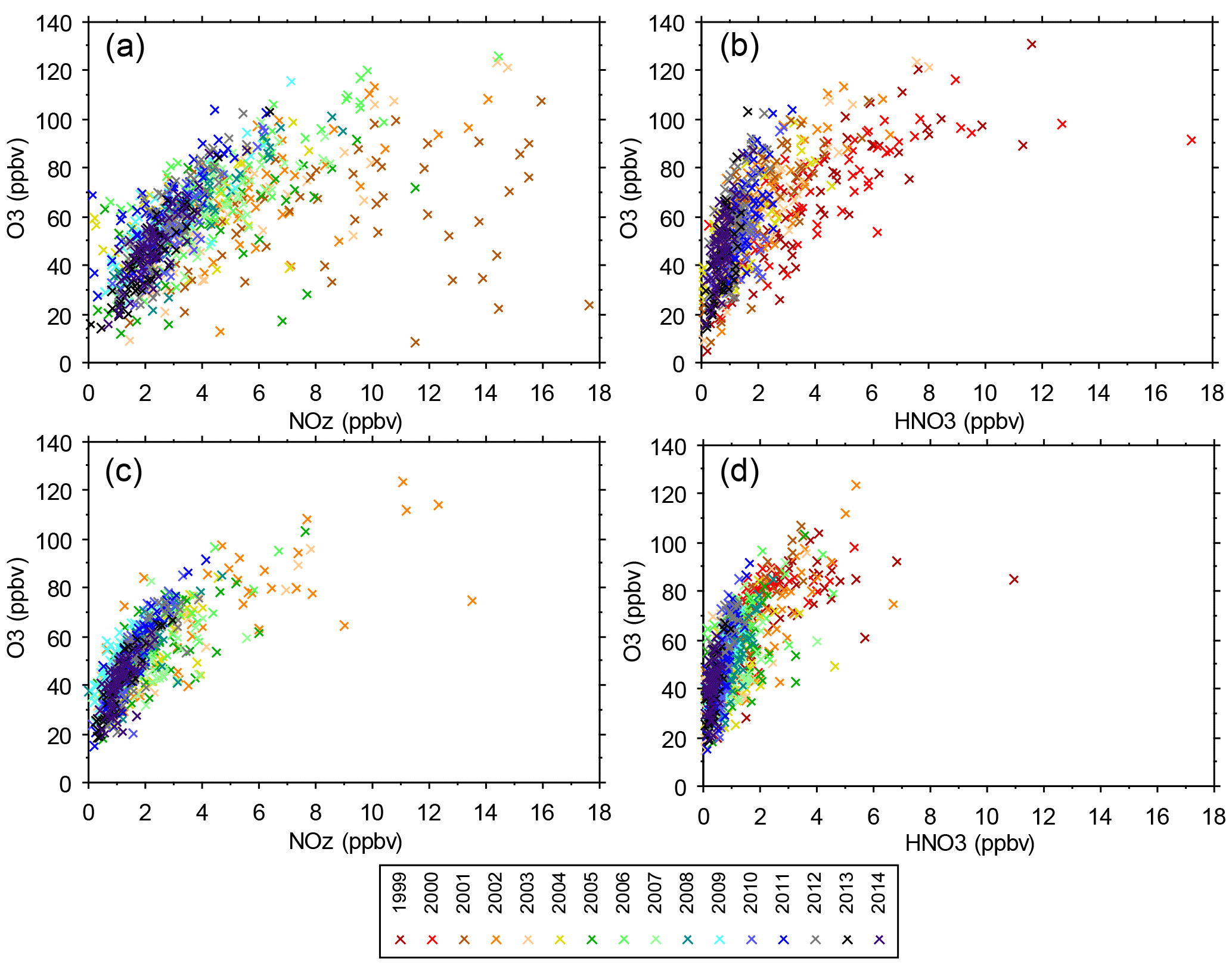
Figure 8 (a) O₃ vs. NO_z at JST, (b) O₃ vs. HNO₃ at JST, (c) O₃ vs. NO_z at YRK, and (d) O₃ vs. HNO₃ at YRK. Each point is the 14:00–15:00 hourly average on 1 day, limited to days in June or July and delineated by year. The 2001 and 2002 NO_z data may be biased high due to lower NO₂ mixing ratios obtained by the instrumentation used at that time (Fig. S2).

Mean mixing ratios of ethylene and aromatic compounds vary substantially between urban and rural sites and exhibit less, and a different, seasonal variation than does isoprene, peaking in the fall rather than in the summer (compare Figs. 6, S5, S6). Daily-average mixing ratios of toluene, xylenes, and ethylene decline over the years, consistent with regulatory reductions of anthropogenic VOC emissions (Figs. S5, S6). Seasonal variations in ambient mixing ratios and trends in the anthropogenic emissions of aromatic compounds are expected to influence O₃ mixing ratios and production in urban settings (rural anthropogenic VOC mixing ratios are lower but detectable).

The 24 h average VOC mixing ratios are of somewhat limited value for showing the influence of VOCs on O₃ formation and accumulation. VOC influence is dependent on NO_x mixing ratios, which vary depending on proximity to emission sources and time of day. Meteorological variability, including diurnal and day-to-day changes in temperature, vertical mixing, cloud cover, photolysis, and air mass transport, further obscures the quantitative effects of VOCs on seasonal and interannual variations of O₃. Influences of anthropogenic VOCs at SEARCH sites have previously been reported (Blanchard et al., 2010b, 2014) and are not analyzed beyond this summary.

4.3 Diurnal variations of O₃, NO_y, NO_z, and HNO₃

Summer (June–August) mean O₃ mixing ratios exhibit characteristic nocturnal minima and midday (noon to 16:00, midpoint ∼ 14:00) maxima at all SEARCH sites (Fig. 7). This diurnal pattern remained essentially the same at both the urban and rural sites from 1999 through 2014, but the daytime maxima decreased. Between 1999 and 2014, the summer mean midday maxima declined by ∼ 30 ppbv at all sites, while nocturnal means exhibited variable responses (Fig. 7). Similar diurnal variations occur throughout the year, with smaller decreases in the mean midday O₃ maxima occurring during seasons other than summer (Figs. S7–S9). By the end of the study period, diurnal O₃ profiles were higher during spring (March through May) than summer at the rural sites (CTR and YRK, Figs. S7 and S8), consistent with the reduction in summer mean monthly daily peak 8 h O₃ averages (Fig. 4). Decreasing summer diurnal mean NO_y, HNO₃, and NO_z mixing ratios were also observed, with a general flattening of the profiles and with the times of maxima remaining consistent (Figs. S10–S12). O₃ changes are discussed in relation to changes in NO_y and NO_z in Sect. 4.4, with emphasis on summer and additional consideration of spring months.

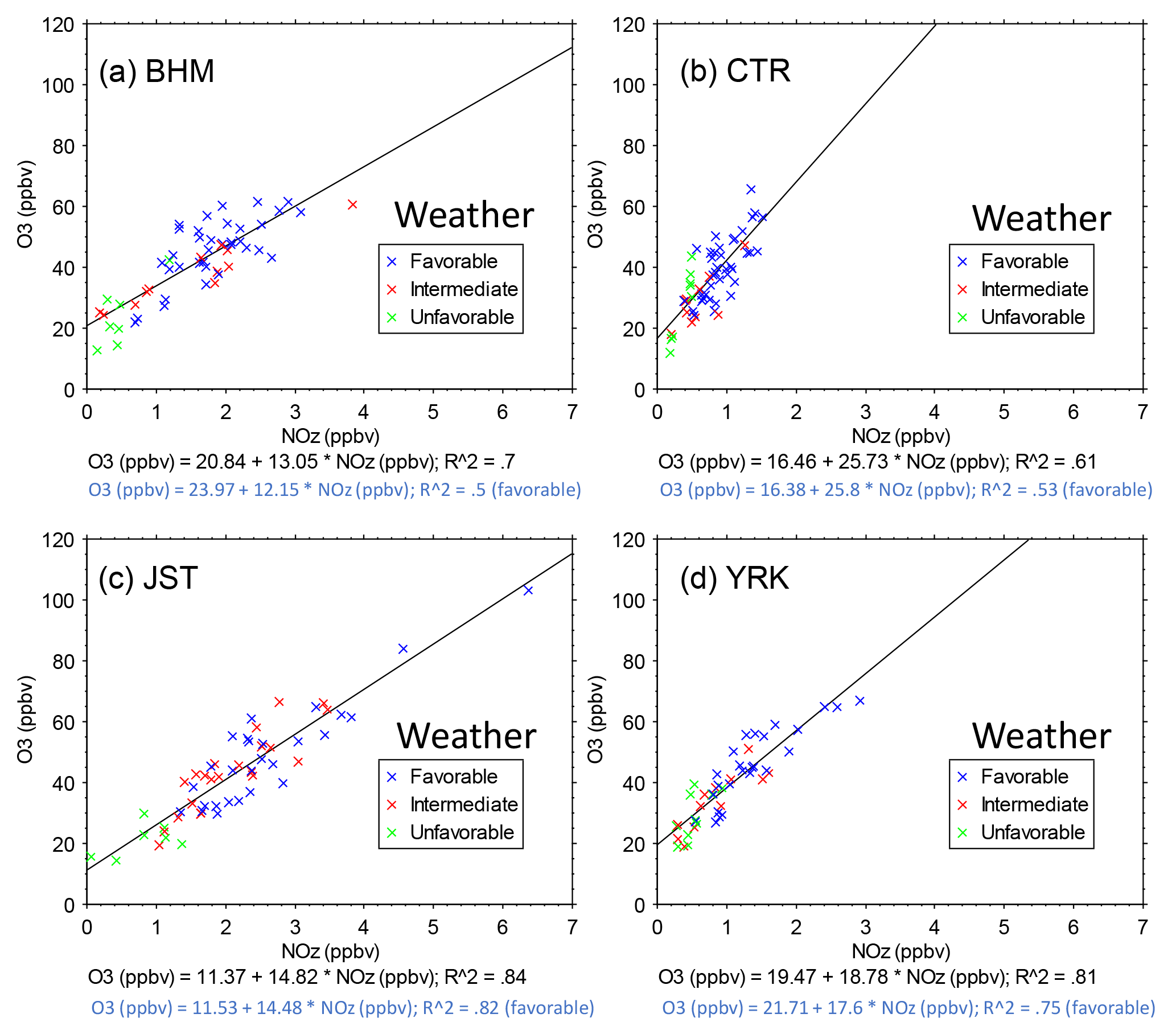
Figure 9 O₃ vs. NO_z during June and July 2013. Each point is the 14:00–15:00 hourly average on 1 day. The data were selected to represent the approximate midpoint of the midday O₃ maxima and to span a period around the summer solstice (∼ −20, ∼ +40 days) when solar radiation is highest on average. The regression slopes show higher rural than urban values: BHM = 13.05 ± 1.19 ppbv ppbv⁻¹, JST = 14.82 ± 0.88 ppbv ppbv⁻¹, YRK = 18.78 ± 1.38 ppbv ppbv⁻¹, and CTR = 25.73 ± 2.76 ppbv ppbv⁻¹. Corresponding regression slopes for O_x vs. NO_z are BHM = 12.00 ± 1.16 ppbv ppbv⁻¹, JST = 13.88,± 0.93 ppbv ppbv⁻¹, YRK = 18.85 ± 1.37 ppbv ppbv⁻¹, and CTR = 25.79 ± 2.79 ppbv ppbv⁻¹. Symbols indicate the favorability of weather to O₃ formation and accumulation: (1) favorable – T > 25 ^∘C, RH < 70 %, and solar radiation > 500 W m⁻²; (2) intermediate – neither favorable nor unfavorable; (3) unfavorable – T < 25 ^∘C, RH > 70 %, and solar radiation < 500 W m⁻². Regression results are shown for all days and for the days with favorable weather.

4.4 Observed relationships between O₃ and NO_z

As discussed above, O₃ mixing ratios vary seasonally and diurnally in response to variations in emissions, weather, background O₃, and other factors. To reduce the influence of seasonal and diurnal variability, this section focuses on mixing ratios of NO_z, HNO₃, and O₃ at 14:00 during June and July. Both temperature and solar radiation are typically high during June and July, and multi-day stagnation events occur frequently in association with high barometric pressure (Blanchard et al., 2013). Exceptions exist during the passage of frontal systems (Blanchard et al., 2013; Fig. S13). The 14:00 hour has the highest, or close to highest, average hourly O₃ for all sites and years (Fig. 7). The atmosphere is well mixed by midday. Over the range of ambient mixing ratios observed across 15 years, the June–July 14:00 O₃ values are distinctly nonlinear in relation to ambient NO_z and HNO₃ mixing ratios (Fig. 8). More variability is evident at urban sites than at rural sites, consistent with influence of urban NO_x and perhaps VOC emissions on O₃. The nonlinearity indicated in Fig. 8 is also evident when the data are restricted to days having the highest peak daily 8 h O₃ mixing ratios (Fig. S14).

4.4.1 Linear models

Linear regressions are fit to the afternoon data by year, as shown in Fig. 9 for 2013 and in Table S4 for all years. During multi-week periods within any summer, all sites exhibit near-linear relationships of midday O₃ to NO_z. Because the ranges of NO_x and NO_z mixing ratios within each year are limited, year-specific relationships are close to linear and linear models are statistically significant. Steeper slopes at rural sites than at urban sites in Fig. 9 suggest that either more O₃ molecules formed per molecule of NO_x consumed in rural locales than in urban areas or that greater losses of NO_z occurred at the rural sites, as discussed below. At all sites, similar results are obtained for regressions of O_x (O₃ + NO₂) vs. NO_z compared with O₃ vs. NO_z (Fig. 9, caption). At 14:00, rural O₃ mixing ratios are nearly identical with O_x mixing ratios and with other metrics (e.g., O₃–[NO_y–NO]) (Fig. S15). At urban sites, 14:00 NO₂ mixing ratios are non-negligible, but this difference alters the intercepts rather than the slopes of the regressions of O_x vs. NO_z compared with O₃ vs. NO_z (Fig. 9). As previously noted (Fig. S13), even during the 2-month periods that we analyzed, the weather is not always conducive to O₃ formation and such days could influence the observed slopes and intercepts. However, regression results restricted to days with weather that favors O₃ formation (as defined in Fig. 9) do not differ from the unrestricted regressions.

Plotting the year-specific (June–July) computed regression slopes versus mean June–July 14:00 NO_z shows significant increases over time as ambient NO_z mixing ratios have decreased, subject to year-to-year variability (Fig. 10, Table S4). Similar urban–rural differences and patterns of increasing regression slopes are also observed when data are restricted to March and April (spring) at YRK and JST (Fig. S16). The results for spring show more variability than the summer year-specific linear models. One key difference between spring and summer days is that cumulative solar radiation between sunrise and 14:00 is greater on summer days than on spring days, presumably fostering greater photochemical extent of reaction and accumulation of O₃ during summer.

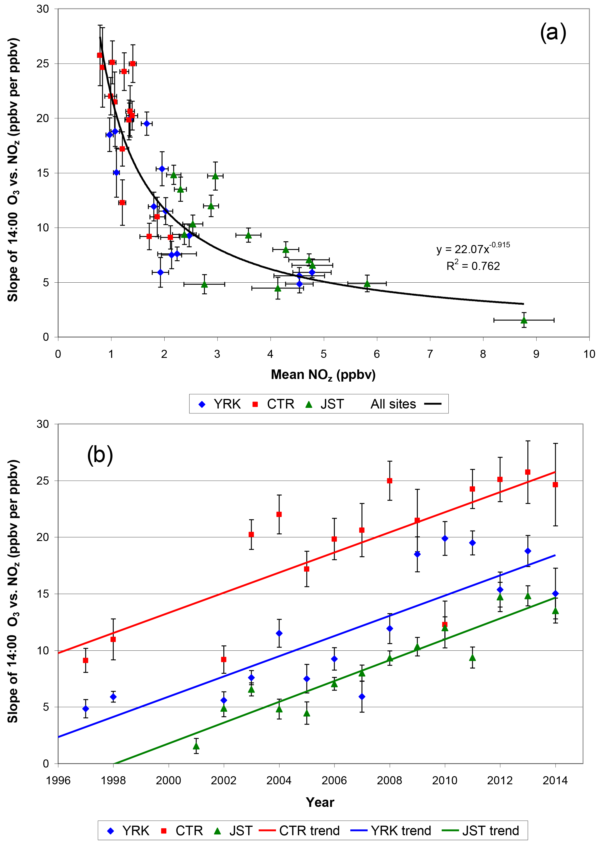
Figure 10 (a) Summer CTR, JST, and YRK slope of daily (14:00) O₃ and NO_z vs. mean (14:00) NO_z mixing ratios and (b) summer regression slope vs. year. NO₂ data were not available for 1999 through 2001. Vertical and horizontal error bars are 1 standard error of the regression slopes and 1 standard error of the NO_z means, respectively. Mean NO_z measurement uncertainty is estimated as 0.2 ppbv (1σ).

The regression slopes determined from 14:00 data could reflect day-to-day differences in transported O₃ if background O₃ is consistently higher on high-O₃ days than on low-O₃ days and NO_z is not (in contrast, random variations in day-to-day background O₃ and NO_z would introduce variations, or scatter, around the regression lines). We checked for an effect of this type by repeating the analyses using differences in mixing ratios. Two sets of difference-based regressions are used: (1) the differences between 14:00 and 10:00 hourly measurements and (2) the differences between 11:00 and 10:00 hourly measurements. The differences are computed for each day to minimize or eliminate the unknown day-specific background levels and are then used in the regressions. These hours were selected to focus on times of day when the atmosphere is well mixed. The morning rise in mixing heights is expected to contribute to increases in the mixing ratios of secondary species as aged air aloft is incorporated into the mixed layer. The most rapid rates of increase in diurnally averaged O₃, NO_z, and HNO₃ values occur between ∼ 08:00 and 12:00 noon local time (Figs. 7, S8–S9). By mid- to late-morning hours during summer, considerable vertical entrainment has occurred, and subsequent changes in the mixing ratios of secondary species likely reflect same-day atmospheric chemical reactions. Computing afternoon–morning differences and late morning–mid-morning differences helps account for day-to-day variations in regional background O₃ but also introduces higher relative uncertainties because four measurements (two differences) are used in the regressions. Results for all three approaches are tabulated in Table S5, by site and year. Like the regressions based on 14:00 measurements, the difference-based regressions indicate that observed slopes have increased over time (Table S5). The difference-based regressions exhibit lower slopes than the non-differenced afternoon regressions, which could be due to lesser statistical fit, or to better accounting for regional background O₃, or to a combination of these factors. The difference-based regressions suggest that O₃–NO_z slopes increased from less than 5 : 1 in the late 1990s and early 2000s to values between 5 : 1 and 10 : 1 after 2010 (Table S5). These lower slope values are consistent with our previous results in which observed O₃–NO_z relationships were determined while also accounting for day-to-day variations in meteorology, which indicated that JST, YRK, and CTR O₃ ∕ NO_z slopes were 3.5, 5.0, and 7.1, respectively, within the range of 1 to 5 ppbv NO_z, for measurements made during March–October of 2002–2011 (Blanchard et al., 2014).

A second potential effect on the temporal changes in the regression slopes could be due to changes in NO₂ measurement methods (previously described); this possibility was checked by using regressions of O₃ vs. HNO₃ (Fig. S17). The results indicate that the relationship in Fig. 10 is not an artifact of changes in NO₂ measurement methods. The record is more complete for the regressions of O₃ vs. HNO₃, because the HNO₃ measurements were made over a longer time than the NO₂ measurements (and the latter are needed for computing NO_z). As shown for YRK, the year-specific slopes of 14:00 O₃ vs. NO_z and for O₃ vs. HNO₃ each increased substantially after about 2008 (Figs. 10, S17). The O₃ vs. NO_z and O₃ vs. HNO₃ regression slopes tend to level out after 2011, and possibly decrease somewhat, but variability is too high to project beyond the observed data ranges (Figs. 10, S17). Similar results are obtained for spring for JST and YRK (Figs. S18 and S19).

Our increases in year-specific slopes of O₃ versus NO_z potentially could be due to increasing losses of NO_z species, especially HNO₃, over the long-term SEARCH record. As previously noted, however, the CASTNET data show declining rates of both wet and dry nitrate deposition since the late 1990s, with no change in the ratio of deposition to emissions (Fig. 1). Therefore, the long-term slope increases cannot be attributed to increasing deposition losses of HNO₃ (whether absolute or fractional). Qualitatively, the CASTNET data suggest that the observed slopes would likely be at least a factor of 2 smaller if adjusted for deposition losses. This adjustment would be comparable to the 1990s studies discussed in Sect. 4.4.2. In Fig. 9, the intercepts of year-specific regressions for 2013 approach 20 ppbv O₃, which could be interpreted as a regional background O₃ level relatively unaffected by local chemistry. These values are lower than those in Fig. 2 and lower than the estimated range of 48 to 59 ppbv for air transported into the Houston area. They are also lower than modeled western non-US-anthropogenic regional background O₃ levels of ∼ 40–50 ppbv (Lefohn et al., 2014; Dolwick et al., 2015) but are consistent with model estimates of non-US-anthropogenic background O₃ less than ∼ 30 ppbv in Atlanta (Lefohn et al., 2014). Since regression intercepts restricted to days with weather that favors O₃ formation do not differ much from the intercepts of the unrestricted regressions (Fig. 9), our low intercepts for recent years do not appear to be linked to meteorological conditions that specifically favor O₃ loss over formation. However, when considered over the full set of years, the O₃–NO_z relationships on the highest O₃ days differ from those on larger subsets of the data (Fig. S14). Possibly, the intercept terms cannot be fully interpreted without additional consideration of O₃ carryover in multi-day episodes, as previously noted. The intercept terms for earlier years are higher than for later years; for example, the intercepts for the YRK regressions range from 27 ± 3 to 42 ± 4 ppbv prior to 2009 (for all but 2 of these years, intercepts are 36–38 ppbv). The intercept terms for earlier years are consistent with 1997–2006 eastern US summer baseline O₃ levels (32 ± 12 ppbv in the absence of continental influences) reported by Chan and Vet (2010).

Higher intercepts during early years could be due to fitting a linear regression to the upper portion or the midrange of the nonlinear relationship between O₃ and NO_z, as shown in Figs. 8 and S14. The nonlinearity and the downward trends in mean NO_z and HNO₃ mixing ratios mean that slopes of regressions computed at higher mean NO_z and HNO₃ mixing ratios should not be extrapolated beyond their range of applicability to the y intercept. Alternatively, the trend toward lower intercepts could reflect declining mixing ratios upwind of the study sites, consistent with documented long-term reductions of ambient O₃ mixing ratios throughout the US (e.g., Chan and Vet, 2010; Lefohn et al., 2010; Paoletti et al., 2014; Simon et al., 2015; Hidy and Blanchard, 2015). As previously discussed, however, regional background O₃ in the southeastern US does not appear to be trending either upward or downward.

4.4.2 Comparisons with observational and modeling studies

The preceding section demonstrates that the slopes of the regressions of O₃ versus NO_z increased over time and examines the potential influence of measurement artifacts, weather, deposition, and pollutant transport on the results; none of these plausible influences adequately explains why the slopes of the regressions of O₃ versus NO_z increased. The increasing slopes appear to indicate that relationships between O₃ and NO_z changed over time, yet the physical processes associated with the changes remain ambiguous. Modeling studies offer insights. Modeling process analysis by Reynolds et al. (2004) for the eastern US predicted that the number of NO cycles (i.e., the ratio of new plus recreated NO to new NO) would increase from 8 to 14 (∼ 75 %) in central (metropolitan) Atlanta and from 9 to 11 (∼ 20 %) northwest of Atlanta in response to a 60 % reduction of NO_x emissions from a 1996 emissions base case. Both the modeled emission reduction (60 %; compare to Fig. 2) and the modeling subregions (central Atlanta, JST; northwest Atlanta, YRK) are directly comparable to our study period and domain. NO cycling is relevant to our regressions of O₃ versus NO_z because an O₃ molecule is produced, with some loss, each time NO cycles through a set of reactions until NO cycling terminates in reaction products that are components of NO_z (e.g., HNO₃, PAN). Thus, the observed increases in the slopes of the regressions of O₃ versus NO_z are directionally consistent with modeling predictions but larger than the predicted 20–75 % increases in NO cycling.

The data were selected to represent periods that have consistent weather from day to day to minimize the influence of meteorological variability, and regressions of subsets of the data yield slopes and intercepts comparable to those based on all days of June and July (Fig. 9). However, the observed O₃ decreases that have occurred in the region (Figs. 2 and 3) could not have occurred if O₃ formation rates increased by factors of ∼ 3 to 4 (as suggested by Fig. 10) or even by a factor of 2 (Table S5), since NO_x emissions declined by ∼ 60 %, or ∼ 5 % per year over 20 years (Fig. 1; Hidy et al., 2014). This consideration suggests that increased NO cycling, while likely linked with our observational results, cannot be the only factor involved. The regression slopes are nonetheless consistent with related studies when a basis for comparison exists.

The SEARCH-observed afternoon slope values of ∼ 5 : 1 prior to 2003–2007 are comparable to, or lower than, similar regression results obtained in studies during the 1990s – which showed observed summer slope values of 11 : 1 in rural Georgia in 1991 (Kleinman et al., 1994); 8.5 : 1 at rural eastern sites (Trainer et al., 1993); 7 : 1 near Birmingham, AL, in 1992 (Trainer et al., 1995); 5.7 : 1 near Nashville, TN, in 1995 (Sillman et al., 1998); and 4.7 : 1 near Nashville, TN, in 1999 (Zaveri et al., 2003) – and to modeling results and observations with composite regression slope values of 6.7 and 7.6, respectively, within the afternoon planetary boundary layer in the eastern US during the summer of 2002 (Godowitch et al., 2011). The SEARCH regression slope values prior to 2003–2007 are, as expected, higher than other 1990s values that were corrected for deposition losses, which, for example, yielded adjusted estimated values between 3 : 1 and 5 : 1 near Nashville in 1995 (Nunnermacker et al., 1998; St. John et al., 1998; Sillman et al., 1998). Our higher observed slope values after 2010 are consistent with aircraft measurements made in the southeast in August and September 2013, which show an O_x (= O₃ + NO₂) versus NO_z slope of 17.4, and they are also consistent with model calculations, which show slopes of 14.1 to 16.7 (Travis et al., 2016). Consistent with our regressions, Travis et al. (2016) did not adjust for variations in background O₃ and NO_z. For comparability, we note that our O₃ versus NO_z regression slopes were 13.1 to 18.8 (±1.2 to 1.4) in June and July 2013 at three of four sites (25.7 ± 2.8 at the fourth site, which is the most rural in character) and our O_x versus NO_z slopes were 12.0 to 18.9 (±1.2 to 1.4) at three of the four sites (25.8 ± 2.8 at the fourth site). The increase in recently observed slope values that we report is therefore supported by the 2013 data of Travis et al. (2016). Our apparently high regression slope values are comparable to observations that averaged 12.9 in ship plumes and 33.5 in assumed background marine air, as reported by Kim et al. (2016) using data from a 2002 study of ship emission plumes off the coast of southern California, though the specific conditions associated with these two studies are different from ours and thus limit the applicability of the comparisons.

The increase in regression slopes with decreasing ambient NO_x and NO_z is also directionally consistent with computations by Liu et al. (1987), which showed increasing OPE as NO_x declines. The numerical results of the modeling calculations by Liu et al. (1987) are specific to the modeled conditions, which represented complete oxidation of VOCs over a period of months. However, increases in model-predicted NO_x OPE with declining NO_x result from multiple factors, such as radical reactions involving VOCs and NO_x, that are pertinent to other situations (Lin et al., 1988).

In contrast to southern California, where Pollack et al. (2013) reported a shift from PAN to HNO₃ production, the SEARCH data do not definitively show a changing fraction of HNO₃ relative to NO_y. Increasing formation of PAN (which regenerates NO₂) and decreasing formation of HNO₃ (which terminates cycling between NO and NO₂) could facilitate O₃ accumulation as ambient NO_x and NO_z mixing ratios continue to decline. Since the long-term SEARCH data record does not include measurements of PAN, this possible effect could not be investigated.

5 Implications

Observed relationships between O₃ and NO_y species provide insight into the potential for future O₃ changes in the southeastern US. Sustained urban and rural measurements of O₃ and precursors, as carried out in the SEARCH study, show O₃ changes in response to emission precursor reductions in a region having unusually high emissions of natural volatile organic compounds. Anthropogenic NO_x and VOC emissions are each expected to continue to decline. O₃ in the southeast is sensitive to NO_x, and this sensitivity is expected to strengthen with reduced anthropogenic NO_x and VOC emissions. The SEARCH observations could be used for retrospective testing of model projections to enhance the credibility of the models.

6 Conclusions

This study illustrates the value of consistent, long-term measurements of O₃ and reactive nitrogen made at both urban and rural sites for characterizing the response of O₃ to changes in precursor emissions. In the southeastern United States, O₃ production is sensitive to nitrogen oxides; long-term observations document increasing sensitivity with declining NO_x emissions and ambient mixing ratios. Over a period of 14 years, the rate of change in afternoon O₃ mixing ratios with respect to observed mixing ratios of NO_z increased at urban and rural monitoring sites as ambient NO_y mixing ratios declined. In addition, changes in the relative importance of chemical reactions that yield HNO₃ compared with PAN could have played a role in altering O₃ accumulation. The highest peak daily 8 h average O₃ mixing ratios tended to occur in summer, but the study provides some evidence for a recent shift in the frequency of maxima to spring in some locations. Maintaining measurements of O₃, NO, NO₂, and NO_y and adding routine observations of HNO₃ and organonitrates would assist in clarifying future changes of ΔO₃ ∕ ΔNO_z. Long-term documentation and analysis of trends in O₃ mixing ratios in relation to NO_x emission reductions and decreases in ambient reactive nitrogen concentrations yields opportunities for obtaining insights about ambient O₃ reductions that complement and corroborate air quality modeling predictions and add substantially to the “weight-of-evidence” approach for air quality management adopted by the US government after 2000.