the Creative Commons Attribution 4.0 License.
the Creative Commons Attribution 4.0 License.
 | 31 May 2018
Multiple symptoms of total ozone recovery inside the Antarctic vortex during austral spring
Andrea Pazmiño
Sophie Godin-Beekmann
Alain Hauchecorne
Chantal Claud
Sergey Khaykin
Florence Goutail
Elian Wolfram
Jacobo Salvador
Eduardo Quel
The long-term evolution of total ozone column inside the Antarctic polar vortex is investigated over the 1980–2017 period. Trend analyses are performed using a multilinear regression (MLR) model based on various proxies for the evaluation of ozone interannual variability (heat flux, quasi-biennial oscillation, solar flux, Antarctic oscillation and aerosols). Annual total ozone column measurements corresponding to the mean monthly values inside the vortex in September and during the period of maximum ozone depletion from 15 September to 15 October are used. Total ozone columns from the Multi-Sensor Reanalysis version 2 (MSR-2) dataset and from a combined record based on TOMS and OMI satellite datasets with gaps filled by MSR-2 (1993–1995) are considered in the study. Ozone trends are computed by a piece-wise trend (PWT) proxy that includes two linear functions before and after the turnaround year in 2001 and a parabolic function to account for the saturation of the polar ozone destruction. In order to evaluate average total ozone within the vortex, two classification methods are used, based on the potential vorticity gradient as a function of equivalent latitude. The first standard one considers this gradient at a single isentropic level (475 or 550 K), while the second one uses a range of isentropic levels between 400 and 600 K. The regression model includes a new proxy (GRAD) linked to the gradient of potential vorticity as a function of equivalent latitude and representing the stability of the vortex during the studied month. The determination coefficient (R2) between observations and modelled values increases by ∼ 0.05 when this proxy is included in the MLR model. Highest R2 (0.92–0.95) and minimum residuals are obtained for the second classification method for both datasets and months.
Trends in September over the 2001–2017 period are statistically significant at 2σ level with values ranging between 1.84 ± 1.03 and 2.83 ± 1.48 DU yr−1 depending on the methods and considered proxies. This result confirms the recent studies of Antarctic ozone healing during that month. Trends from 2001 are 2 to 3 times smaller than before the turnaround year, as expected from the response to the slowly ozone-depleting substances decrease in polar regions.
For the first time, significant trends are found for the period of maximum ozone depletion. Estimated trends from 2001 for the 15 September–15 October period over 2001–2017 vary from 1.21 ± 0.83 to 1.96 DU ± 0.99 yr−1 and are significant at 2σ level.
MLR analysis is also applied to the ozone mass deficit (OMD) metric for both periods, considering a threshold at 220 DU and total ozone columns south of 60∘ S. Significant trend values are observed for all cases and periods. A decrease of OMD of 0.86 ± 0.36 and 0.65 ± 0.33 Mt yr−1 since 2001 is observed in September and 15 September–15 October, respectively.
Ozone recovery is also confirmed by a steady decrease of the relative area of total ozone values lower than 175 DU within the vortex in the 15 September–15 October period since 2010 and a delay in the occurrence of ozone levels below 125 DU since 2005.
- Article
(736 KB) - Full-text XML
-
Supplement
(130 KB) - BibTeX
- EndNote


The evolution of total ozone content (TOC) in Antarctica during austral spring is strongly linked to the important stratospheric ozone decline that was highlighted for the first time by Chubachi et al. (1985) and Farman et al. (1985). Nowadays the photochemical and microphysical processes leading to the massive and seasonal destruction of ozone in polar regions are well understood. The latest Ozone Assessment Reports (WMO, 2007, 2011, 2014) have confirmed the stabilization of ozone loss in Antarctica since 2000. The challenge now is to assess the impact of the observed reduction in the concentration of ozone-depleting substances (ODSs) (evaluated in the polar regions to ∼ 10 % in 2013 from the peak values in 2000; WMO, 2014) on the amplitude of the ozone destruction every year. During the last decade, several studies have been carried out to quantify a possible increase in total ozone column in the Antarctic polar vortex in spring directly linked to this decrease in the polar stratosphere. Most analyses use multilinear regression (MLR) models with different proxies to represent the interannual variability of ozone as a function of the 11-year solar cycle, the quasi-biennial oscillation (QBO), volcanic aerosols (Aer) or eddy heat flux (HF) (Salby et al., 2012; Kuttippurath et al., 2013; de Laat et al., 2015). These studies generally show a significant increase of TOC since 2000 for the September–November averaged period but they differ on the proxies used for the quantification of ozone interannual variability. De Laat et al. (2015) used a “big data” ensemble approach to calculate trends. Several scenarios were considered for the period over which the ozone record is calculated and for the different proxy records. They found that the significance of trends could vary from negligible to 100 % significant at 2σ levels depending on the scenario considered. They have also determined the optimal proxy records and ozone record scenarios to obtain the best regression. The limitation of MLR analysis is that only formal statistical error of trend is estimated and structural uncertainties linked to the single and arbitrary combination of proxies is not taken into account. De Laat et al. (2017) inferred trend values from daily ozone mass deficit (OMD) computed from a multi-sensor reanalysis (MSR) dataset without using any model but filtering the anomalous years with low polar stratospheric cloud (PSC) volume. The authors found positive and highly significant trend of OMD since 2000.
Solomon et al. (2016) evaluated trends in total ozone and ozone profiles records as well as healing characteristics by combining measurements (satellites and ozonesondes) and the Specified Dynamics version of the Whole Atmosphere Community Climate Model (SD-WACCM). They found a significant healing in September but not in October, during which ozone depletion is largest in the first 2 weeks. They also explain the difficulty of estimating the trend in October because the large variability of ozone linked to temperature variations and transport. The baroclinicity of the polar vortex in October and its displacement from the geographic pole can also contribute to the variability of the total ozone series averaged during the month of October.
The direct link observed between positive trends of total ozone within the polar vortex and the reduction of ODSs remains open to debate, given the natural variability of the Antarctic vortex and the possible contribution of greenhouse gases to the trends (Chipperfield et al., 2017).
The purpose of this paper is to provide an update of the ozone evolution inside the Antarctic vortex during the last decades, taking into account the vortex baroclinicity. The main aim is to determine the different contributions to ozone interannual variability and to estimate the post-2001 total ozone trend and related significance for different periods: September, which corresponds to the period of fastest development of catalytic photochemical ozone destruction, and mid-September to mid-October when the maximum ozone loss is reached.
This paper is organized as follows. Ozone datasets from satellites and MSR are presented in Sect. 2 and the description of the method used for total ozone column classification inside the vortex in Sect. 3. The influence of vortex baroclinicity on total ozone column inside the vortex is assessed in Sect. 4 by using a new classification method compared to standard ones based on a single isentropic level. Ozone trends before and after the turnaround year calculated using a multi-regression model for September and mid-September to mid-October are presented and discussed in Sect. 5. Results of trends using OMD records as a metric are also presented. The temporal evolution of the amount of very low total ozone values inside the vortex is evaluated in Sect. 6. Conclusions are finally presented in Sect. 7.
Total ozone global fields from satellite observations – Total Ozone Mapping Spectrometer (TOMS) and Ozone Monitoring Instrument (OMI) – and MSR are used in this study to cross-check trend estimation before and after a turnaround year over the 1980–2017 period.
2.1 Space-borne observations
Total ozone column data series of NASA's TOMS instrument on board Nimbus-7 (N7) and Earth Probe (EP) between 1980 and 2004 are used. The instrument is a single monochromator that was designed for near-nadir measurements of the total ozone column (e.g. McPeters et al., 1998). TOMS measures the backscattering of solar radiation by the Earth's atmosphere in six 1 nm bands of ultraviolet wavelength between 306 to 380 nm, more or less absorbed by ozone. Total ozone column is inferred from the ratio of two wavelengths, 317.5 nm strongly absorbed by ozone and 331.2 nm weakly absorbed (Bhartia and Wellemeyer, 2002). Level 3 gridded TV8 data of 1.0∘ (lat) × 1.25∘ (long) of total ozone columns of TOMS were used in this work and are available from the Goddard Earth Sciences Distributed Information and Services Center (GES DISC) in simple ASCII format in the NASA anonymous ftp site (ftp://toms.gsfc.nasa.gov/, last access: 27 May 2018)
Ozone total column observations of OMI on board Aura satellite are also used to continue TOMS measurements from 2005 to 2017. The OMI instrument is a nadir-viewing hyperspectral imaging in a push-broom mode. OMI measures the solar backscatter radiation in the complete spectrum of the ultraviolet–visible wavelength range (270–500 nm) with 0.5 nm spectral resolution (Levelt et al., 2006). Total ozone column used in this work was retrieved using TV8 algorithm, hereafter referred to as OMIT in order to maintain continuity with TOMS data record (McPeters et al., 2008). Level 3 daily gridded data of OMI with better spatial resolution (1.0∘ × 1.0∘) than TOMS are used. Data are also available on NASA's anonymous ftp site.
The total ozone column data series was combined by using specific satellite data over the following periods: TOMS-N7 (1980–1992), TOMS-EP (1996–2004) and OMI (2005–2017). Note that data of 1993–1995 are sparse or missing for the September–October period. In order to complete the data series, total ozone columns of Multi-Sensor Reanalysis version 2 (MSR-2) were used (see Sect. 2.2). Since TOMS and OMI UV sensors do not receive enough UV light in early September, originating from regions not illuminated by the Sun (from 77 to 82.5∘ S up to mid-September), these regions were not considered to compute the total ozone mean value in MSR-2 data.
TOMS, OMI and MSR-2 data series have previously been used in different scientific studies of ozone recovery in the southern polar region (Salby et al., 2012; Kuttippurath et al., 2013; Solomon et al., 2016). Hereafter the 1980–2017 composite satellite total ozone series will be called SAT.
2.2 Multi-sensor reanalysis
Ozone MSR-2 provides global assimilated ozone fields for the period 1980–2017 based on 14 satellite datasets (van der A et al., 2015). The 14 polar-orbiting satellites measuring in the near-ultraviolet Huggins band were corrected to construct a merged satellite data series that are assimilated within the chemistry–transport assimilation model TM3-DAM to obtain MSR-2 data (see van der A et al., 2010, for a detailed description and van der A et al., 2015, for last improvements of the assimilation model). Corrections of offset, trends and variations of solar zenith angle and temperature in the stratosphere were computed in satellite datasets by comparisons with individual ground-based Dobson and Brewer measurements from World Ozone and Ultraviolet Data Center (WOUDC). Those corrections are specified in van der A et al. (2015), Table 2.
Table 1Information of proxies (source, characteristics and time window for the mean yearly value).
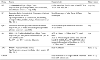
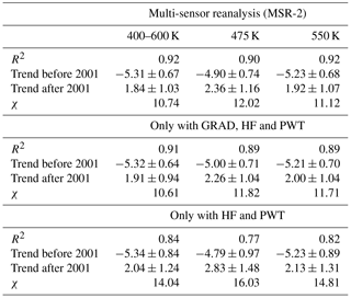
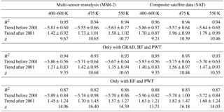
Table 2Coefficient of determination R2 and trends ±2σ in DU yr−1 before and after the turnaround year 2001 derived from multi-regression model using as input MSR-2 (1980–2017) total ozone anomalies inside the vortex for September using three classification methods described in Sect. 3.2. The residual is represented in DU by , where obsi and modi correspond to observations and model monthly mean, n the number of years and m the number of parameters fitted as in Weber et al. (2018).
Daily gridded forecast ozone data of MSR-2 at 12:00 UTC and spatial resolution of 0.5∘ × 0.5∘ were used in this work and they are available from the Tropospheric Emission Monitoring Internet Service (TEMIS) of KNMI/ESA (http://www.temis.nl/protocols/o3field/data/msr2/, last access: 27 May 2018).
Different studies on trends in the Southern Hemisphere have used MSR-2 data (Kuttippurath et al., 2013; de Laat et al., 2015, 2017). Hereafter the 1980–2017 ozone series will be called MSR-2.
In order to consider total ozone columns only within the polar vortex, the data classification is performed by evaluating the vortex's position at different isentropic levels from 1 May to 31 December, each year. Two classification methods are then applied in order to evaluate the impact of baroclinicity of the vortex on the averaged total ozone columns in both studied depletion periods. The first one is based on a single isentropic level, while the second one considers a range of isentropic levels.
3.1 Vortex position
For each day of the studied periods, the vortex position is determined by using a 2-D quasi-conservative coordinate system (equivalent latitude–potential temperature) described by McIntyre and Palmer (1984), where the pole in equivalent latitude (EL) corresponds to the position of maximum potential vorticity (PV). This conservative system is computed from PV field simulated by the Modélisation Isentrope du transport Mésoéchelle de l'Ozone Stratosphérique par Advection (MIMOSA) PV advection model (Hauchecorne et al., 2002). The model was forced by ERA-Interim (Dee et al., 2011) meteorological data (2.5∘ × 2.5∘) of European Centre for Medium-Range Weather Forecasts (ECMWF). Daily advected PV fields (1∘ × 1∘) on the 30–90∘ S latitude band at 12:00 UTC are used to calculate EL on the isentropic level range between 400 and 600 K with a step of 25 K.
Following Nash et al. (1996), PV is evaluated as a function of EL and three particular regions are identified: inside the vortex, characterized by high PV values, at the vortex edge, corresponding to high PV gradients and outside the vortex (or surf zone) with small PV values. The limit of the vortex corresponds to the EL of maximum PV gradient, weighted by the wind module. This limit is subsequently smoothed temporally with a moving average of 5 days to reduce the noise in the vortex edge data series.
3.2 Methodology for classification
The Nash criterion was already used in several studies to distinguish measurements (ozone profiles and total columns) inside and outside the vortex in the Southern Hemisphere (Godin et al., 2001; Bodeker et al., 2002; Pazmiño et al., 2005, 2008; Kuttippurath et al., 2013, 2015). In the case of total columns, measurements were considered inside the vortex when their corresponding EL was larger than the EL of the vortex limit at a specific isentropic level (e.g. 550 K, Bodeker et al., 2002; Pazmiño et al., 2005). However, this “standard” method does not take into account the baroclinicity of the vortex. It can result in the classification of total ozone columns inside the vortex while partial columns below or above the selected isentropic level are outside the vortex. The total ozone column may thus not represent the ozone behaviour inside the vortex. In order to consider possible vortex baroclinicity, another approach is used, where vortex classification at different isentropic levels is considered at the same time. For this second approach, the range of selected isentropic levels is chosen in the altitude region of maximum ozone depletion: from 400 to 600 K with a step of 25 K. The same nine isentropic levels considered for 400–600 K range classification are applied each year.
In order to illustrate the impact of vortex baroclinicity on the classification of total ozone column inside the vortex, Fig. 1 shows MSR-2 total ozone fields on 7 October 2012, with the vortex position computed at different isentropic levels superimposed. The vortex position curves are represented by black to light grey colours. On this particular day, the region classified inside the vortex in the 400–600 K range is limited by the vortex position at 400 K (black line) towards west Antarctic coast and Palmer Peninsula and at 600 K (light grey line) towards the east Antarctic coast. The white dot marks in Fig. 1 show the limit of the region considered in this new classification. In the case of standard classification using a single level at 475 or 550 K, the region estimated as inside the vortex consists of an area with total ozone columns larger than 400 DU. These areas are not considered in the classification using several isentropic levels between 400 and 600 K. Regions where total ozone columns are lower than 220 DU are taken into account by the classification at all the isentropic levels. A daily mean total ozone column of 213.4 DU was computed inside the vortex using this new classification method. The standard classification estimates a 40 and 20 DU larger ozone average values at 475 and 550 K, respectively, on that day.

Figure 1Total ozone (DU) from MSR-2 on 7 October 2012 at 12:00 UTC. Vortex edge position at different isentropic levels are added to the map and represented by black to light grey lines. White dot marks identify the region considered inside the vortex using the 400–600 K range classification.
Both methods of classification described in the previous section were applied to satellite composite total ozone data series SAT and MSR-2 reanalysis at each grid point. For each year, daily mean total ozone amount inside the vortex was averaged over two periods: the whole month of September and the period of maximum ozone depletion between 15 September and 15 October. Figure 2 shows the evolution of total ozone average inside the vortex for the 15 September–15 October period between 1980 and 2017 for the MSR-2 data series computed with the standard classification method based on the single isentropic level (475 and 550 K) and with the second method using the 400–600 K range of isentropic levels. Error bars represent the 2σ standard error. Similar interannual total ozone variability is observed for the time series obtained by the different methods. The correlation coefficients between the range method and the standard one at 475 and 550 K are 0.98 and 0.99, respectively. Despite these good correlations, the data series are significantly different at the 2σ level. Larger ozone values are found with the standard method, especially for the 475 K level, which shows a mean difference with the TOC time series based on the range method of ∼ 15 % over the whole analysis period. Three years stand out in the comparison – 1995, 1999 and 2011 – during which the inside vortex region was systematically larger at 475 K compared to higher isentropic levels during the period. Similar results are observed for September (not shown). In this work, the second method is preferred since it takes into account the ozone loss at different isentropic levels, which strongly impacts the total column.
MSR-2 total ozone time series obtained in September and 15 September–15 October with the range classification method are displayed in Fig. 3. September presents ∼ 8 % larger ozone mean values than the 15 September–15 October period. Similar interannual variability is observed between the two periods as shown by the correlation coefficient of 0.98. The last 4 years present very similar ozone values of around 205 DU in September, while during the 15 September–15 October period they show larger variability.
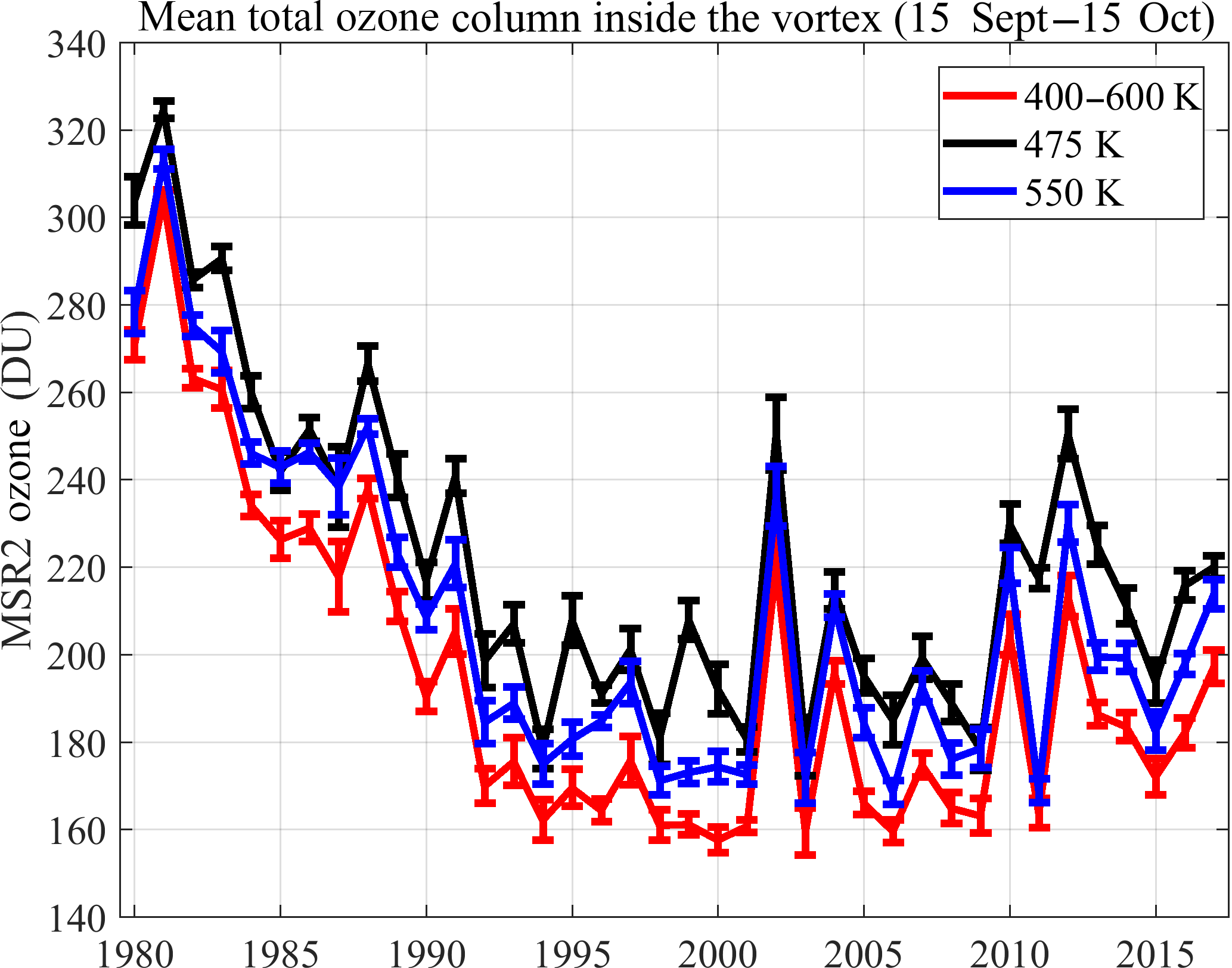
Figure 2Evolution of total ozone of MSR-2 dataset inside the vortex averaged each year on 15 September–15 October period for different classifications: standard method at 475 and 550 K represented by black and blue lines, respectively, and method considering the 400–600 K altitude range by the red line. Error bars represent twice the standard error.
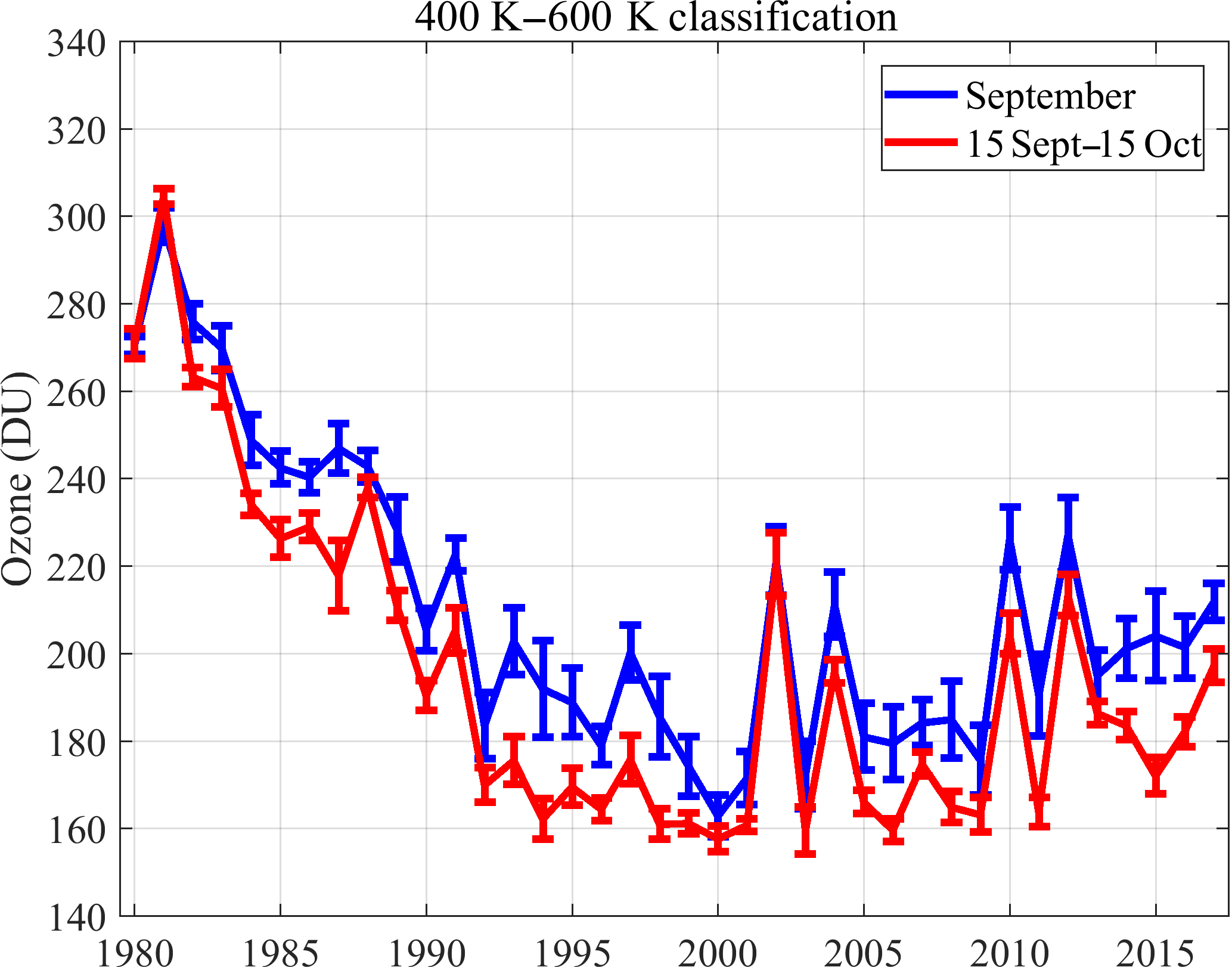
Figure 3As in Fig. 2 but only for 400–600 K classification on different periods: September and mid-September to mid-October. Error bars represent 2σ.
MSR-2 total ozone data series inside the vortex are compared to SAT series as shown in Fig. 4, which displays the relative difference between MSR-2 and SAT for the 400–600 K range classification. Differences of about ±0.5 % are observed in the 1980s. Small differences are expected during this period since only TOMS data are used in both datasets until 1993. In the 1993–1995 period discrepancies between both curves are only due to the differences in the selection of MSR-2 data for the SAT record in order to have similar spatial coverage as the data from the other instruments incorporated in the SAT time series. These differences varying between −1 and 0.5 % represent an estimation of the impact of reduced spatial coverage in SAT dataset on the averaged total ozone level in September. The 15 September–15 October period presents negligible differences. The addition of GOME (1996–2005) in MSR-2 assimilation could explain the discrepancies with the SAT dataset that considers only TOMS-EP. From 2001, differences are larger and generally positive, reaching ∼ 5 % in September and ∼ 3 % in the 15 September–15 October period. These increased differences are especially visible during the period where data from instruments on board the ENVISAT platform (e.g. SCIAMACHY) are assimilated in the MSR-2 record. Overall, values in September present a mean bias of 1.3 % (dash blue line in Fig. 4) and during 15 September–15 October a smaller bias value of 0.5 % (dash red line in Fig. 4). Temporal evolution of the differences, e.g. negative trend in the 1980s and positive trend in the 2000s, can have an impact on the long-term ozone trends retrieved from both records. In general, differences between SAT and MSR-2 records are caused by MSR-2 starting to use multiple satellite total ozone columns records after 1996, procedures in MSR-2 to account for inter-instrument differences and data assimilation methodology that allows for filling gaps (van der A et al., 2015).
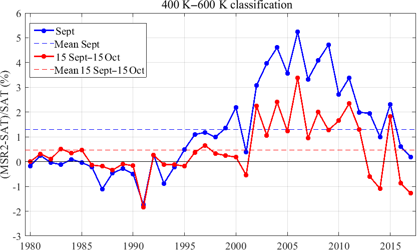
Figure 4Relative difference between MSR-2 and SAT mean total ozone inside the vortex for September (blue curve) and 15 September–15 October (red curve) periods. Horizontal dash lines correspond to the mean bias between data series.
Despite the differences between those datasets, one purpose of this work was to analyse, in the same way, satellite data such as those included in the SAT record without any correction or adjustment and the MSR-2 record, which accounts for inter-instrument differences using ground-based total column data. Due to the larger differences observed between both datasets in September, especially in the 1995–2010 period, which may have an impact on trend analysis, it was decided to retrieve trends from the SAT dataset in the 15 September–15 October only.
In the next section, ozone data series based on the different classification methods are used to evaluate the impact of vortex baroclinicity on ozone trends inside the vortex for both studied periods.
5.1 Method
In order to evaluate ozone recovery in Antarctica, estimation of trends before and after 2001 were calculated using a multi-regression model (Nair et al., 2013) updated from the AMOUNTS (Adaptative Model for Unambiguous Trend Survey) model (Hauchecorne et al., 1991; Kerzenmacher et al., 2006). Different common explanatory variables such as eddy HF, solar flux (SF), QBO, Aer and Antarctic oscillation (AAO) are used to explain total ozone variability over the 1980–2017 period. These proxies were widely applied in different trend studies (e.g. de Laat et al., 2015, and references herein). The ODS contribution to long-term trend in ozone is represented by piece-wise trend (PWT) functions. The total ozone variability (Y) can be expressed following Eq. (1):
where t is year from 1980 to 2017, K is a constant, Cproxy are the regression coefficients of the respective proxies mentioned above and ∈(t) is the total ozone residuals. Table 1 shows the respective information for each proxy: source, specific characteristics and time window where proxy values are averaged to represent the respective year value. QBO effect on ozone variability is estimated using two proxies at 30 hPa (QBO30) and 10 hPa (QBO10), which are out of phase by (Steinbrecht et al., 2003). The HF proxy corresponds to the average over the August–September period of the 45-day mean heat flux in the 45–75∘ S latitude range at 70 hPa from MERRA-2 analyses. The time window of August–September is selected for computing the mean HF, following de Laat et al. (2015) recommendation to obtain the best regression results. For the Aer term, a merged proxy of monthly aerosol optical depth (AOD) is computed from updated Sato et al. (1993) dataset for the 1980–1990 period and from four satellite data series (SAGE II, OSIRIS, CALIOP and OMPS) for the 1991–2017 period. AOD datasets are averaged over the 40–65∘ S zonal region in the 15–30 km altitude range. Updated Sato et al. data are obtained from NASA monthly AOD at 550 nm. The satellite AOD data over 1991–2017 period were computed at 532 nm. The Sato et al. dataset was converted to 532 nm according to Khaykin et al. (2017). The merged AOD proxy was obtained by normalizing the Sato et al. time series to the SAGE II data in December 1991. The regression code uses the AOD values in April before the complete formation of the vortex in order to avoid possible contamination of aerosols satellite data by PSCs. The April AOD proxy is represented by a bold black line in Fig. 5 together with Sato et al. (1993) and satellites datasets for the 1991–2017 period.

Figure 5Time series of April monthly mean AOD at 532 nm within 40–65∘ S and 15–30 km of normalized Sato et al. (1993) dataset (see main text) and from satellites (SAGE II, OSIRIS, CALIOP, OMPS). The corresponding merged data are represented by the bold line.
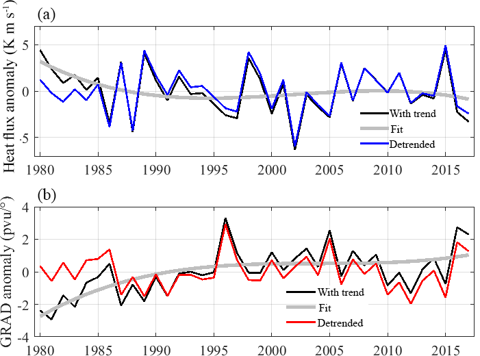
Figure 6Heat flux (a) and gradient (GRAD) (b) anomalies for the 15 September–15 October period: before removing a polynomial fit of third order (black line), the fit (grey line) and after removing the fit (blue/red line).
A new GRAD(t) proxy was developed in order to take into account the stability of the vortex during the studied period. This proxy corresponds to the maximum gradient of PV as a function of EL at 550 K during both studied periods (e.g. September and 15 September–15 October). It is calculated from ERA-Interim data. GRAD and HF proxies are detrended by removing a third-order polynomial fit to minimize correlation with PWT proxies. Figure 6 displays GRAD and HF proxies before and after removing trends. An anticorrelation of ∼ 0.55 between these two proxies is observed with a p value < 0.01, but the addition of GRAD proxy provides a much better agreement between measurements and model, especially during the last decade. The contribution of the GRAD(t) proxy to the improvement of the MLR results is discussed in Sect. 5.2.3.
For the long-term trends, two piece-wise linear trend functions calculated before and after the turnaround year are usually used to estimate the change of slope in the long-term evolution of ozone due to ODSs (e.g. Reinsel et al., 2002; Kuttippurath et al., 2013; de Laat et al., 2015). In this work our modified PWLT model (PWT) uses an additional function in order to take into account the slower growth of ODSs near the turnaround year and the ozone loss saturation effect within the Antarctic polar vortex in October (Yang et al., 2008). The PWT model is represented by Eq. (2):
where Ct11 and Ct2 are the coefficients of the linear functions and Ct12 of the parabolic function. The first period is represented by a linear time proxy t11 and a parabolic time proxy t12. The second period is expressed only by a linear time proxy t2. The proxies are computed as follows:
T0 corresponds to the turnaround year in the considered period. In this work, 2001 was selected as the turnaround year when equivalent effective stratospheric chlorine maximizes for a mean age of air of 5.5 years (Newman et al., 2007). The corresponding value for T0 is 22. Tend corresponds to the number of years considered in the study (38 for 1980–2017). The minimum of the parabolic time proxy t12 is set to the middle of the period before the turnaround year so that the slope of the proxy is zero on that year. In this case the coefficient of t11 (Ct11) can be considered as the linear trend before 2001. After 2001, t11 and t12 are constant and then the linear trend is given by the Ct2 coefficient. Figure 7 represents the evolution of the three piece-wise proxy anomalies normalized by the corresponding standard deviation. The improvement using PWT instead of PWLT is discussed in Sect. 5.2.4.
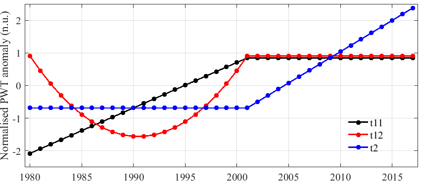
Figure 7Anomalies of the linear functions before and after 2001 (t11 and t2, respectively) and parabolic function (t12) that correspond to the PWT proxy (see Eqs. 2 to 5). Each proxy anomaly is normalized by the corresponding standard deviation.
5.2 Trend results for the averaged total ozone column records
The multi-regression model described in previous section was applied to MSR-2 total ozone anomalies time series computed as monthly total ozone–mean total ozone for the September and 15 September–15 October periods and to SAT for the 15 September–15 October period only. Time series of total ozone data corresponding to the different classification methods described in Sect. 4 were also used to evaluate the impact of vortex baroclinicity on total ozone trends.
5.2.1 September
A rapid decrease of ozone levels occurs within the polar vortex in Antarctica from the last 2 weeks of August to the end of September when the necessary sunlight to start the ozone catalytic destruction cycles is present again above austral polar regions. Important differences in total ozone levels are found inside the vortex between the first and second half of September, with very low values observed mostly during the last week. Although pronounced decrease in total ozone is observed in September, recent publications have used ozone records obtained during this month to detect the ozone recovery (Solomon et al., 2016; Chipperfield et al., 2017; Weber et al., 2018). Those studies use data and/or simulations poleward of ∼ 60∘ S and identify first signs of Antarctic ozone recovery for September but not yet for October due to the larger dynamical variability during that month. In this paper, results from our multi-regression model are evaluated and compared to those previous publications for the September period. Figure 8 illustrates the results of the regression model described in Sect. 5.1 for the MSR-2 total ozone data series inside the vortex using the 400–600 K range classification. The top panel represents the deseasonalized total ozone observations as well as the regressed ozone values. The model results reproduce quite well the interannual variability of measurements except in 2002, when the vortex split in two parts in late September due to a major sudden stratospheric warming (e.g. Allen et al., 2003). Likewise, the year 2000 was characterized by a large ozone hole area (OHA) in September and yielded a relatively high value of residual of ∼ 30 DU on that year. Contributions of the different proxies are shown in the second to fourth panels of Fig. 8. Fitted HF and GRAD were added (black line in second panel of Fig. 8) due to the correlation between both proxies. The model term linked to the HF and GRAD fitted proxy represents the second largest contribution to total ozone interannual variability (∼ 10 % of the total variance) after the PWT proxy which contributes to about 80 % of the total variability. Other proxies (third panel of Fig. 8) represent only 1 % of total ozone variability. Aerosol proxy contributes by ∼ 6 DU in 1992 and ∼ 3 DU in 1983 due to Pinatubo and El Chichón eruptions, respectively. Negligible impact is seen in other years. Fitted QBO (QBO30hPa + QBO10hPa) explains ±5 DU ozone variability. The contributions of SF and AAO proxies are negligible.
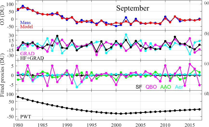
Figure 8Deseasonalized total ozone inside the vortex of MSR-2 series (meas) and regression model (model) for September using 400–600 K classification (a). Contributions of proxies are also shown: heat flux (HF), gradient (GRAD) and the combination of both HF and GRAD (b); solar flux (SF), QBO (QBO at 30 hPa and QBO at 50 hPa), Antarctic oscillation (AAO) and aerosol (Aer) (c); and PWT (d). Ozone anomalies and contributions of proxies are given in DU.
The model explains 92 % of the ozone variability as deduced from the determination coefficient R2. The estimated total ozone trends before and after 2001 are −5.31 ± 0.67 DU yr−1 (−25.2 ± 3.2 % decade−1) and 1.84 ± 1.03 DU yr−1 (8.8 ± 4.9 % decade−1), respectively. Both trends are significant (i.e. statistically different from zero) at 2σ. The 1980–2000 period presents larger depletion rate compared to Weber et al. (2018) (from −12 to −19 % per decade depending on dataset) and comparable rate for the period of recovery (8–10 % decade−1). Comparable values of trends are found when the 475 K classification level is used (−21 ± 3.2 and 10.1 ± 5 % decade−1). The 400–600 K classification allows us to obtain the best agreement between observations and regressed values (larger R2) and lower χ of residuals. Those results are represented in Table 2 for MSR-2 total ozone datasets inside the vortex and for the three classifications analysed in this study. Despite trend values after 2001 for the 475 K classification being larger by about 28 % than for the 400–600 K classification range, trend results between both classifications are not significantly different at 2σ level, suggesting a limited effect of vortex baroclinicity on trend estimation using MLR analysis. The different results in Table 2 generally present a ratio between trends before and after 2001 close to 3, similar to that of ODS trends before and after the peak (Chipperfield et al., 2017). This indicates that the ozone recovery trend could be due to ODS decrease. Nonetheless this trend cannot be reliably associated with chemical processes alone and other processes could also play a role.
Computed trends over the 2001–2017 September period obtained with our model range from 1.84 to 2.36 DU yr−1 for all studied cases. They are all significant at 2σ level. Solomon et al. (2016) found significant total ozone trend of 2.5 ± 1.7 DU yr−1 in September from SBUV and ozonesonde observations and similar results from the Chemistry + Dynamics + Volcanoes (Chem-Dyn-Vol) simulation (2.8 ± 1.6 DU yr−1) using the WACCM. Estimated total ozone trend when only chemistry is considered in the model (Chem-Only) correspond to only half of the final trend (1.3 ± 0.1 DU yr−1).
A simulation test was done to evaluate the pertinence of using other proxies than PWT, HF and GRAD since only these fitted proxies present significant regression coefficient values at 95 % confidence interval. Results are represented in Table 2. Slightly lower determination factor R2 is computed if only PWT, HF and GRAD are considered for September and comparable residual and trends. This results suggest that the others proxies provide marginal improvement to the MLR analysis.
5.2.2 15 September to 15 October
In order to confirm healing of the Antarctic ozone hole, it is important to evaluate trends for the period where the lowest total ozone values are observed inside the vortex e.g. between 15 September and 15 October. The same analysis as for September is thus performed. Figure 9 illustrates the results of regression model for total ozone of MSR-2 data series inside the vortex using the 400–600 K classification. It shows that the interannual variability of measurements is better represented by the model than in September. For that period, the determination coefficient R2 is 0.95 (see also Table 3). As for the September regression, the sum of fitted HF and GRAD proxies (black line in second panel) represents the second largest contribution to total ozone interannual variability (∼ 13 % of the total variance) after the PWT proxy (∼ 80 %) and the last decade of measurement is correctly reproduced by the model. Significant trends of −5.81 ± 0.6 DU yr−1 (−29.8 ± 3 % decade−1) and 1.42 ± 0.92 DU yr−1 (7.3 ± 4.7 % decade−1) are estimated before and after 2001. Similar results are observed if a single level classification is used with larger trend values after 2001 for 475 K. All trend results are comparable within ±2σ. Results based on the SAT record are similar, with slightly larger trend values after 2001. Note that the addition in the MLR analysis of the 2 most recent years (2016–2017), which were characterized by weak ozone holes, changed the significance of the 2001–2017 trend from hardly significant to significant better than 2σ. Results obtained in the 1980–2017 period by the MLR analysis thus show for the first time a significant recovery in the 15 September–15 October period. SF, QBO, Antarctic oscillation and Aer (third panel of Fig. 9) explain ∼ 1 % of the total variance. QBO explains ±3 DU interannual variability and Aer signals amount to ∼ 6 and ∼ 3 DU linked to Pinatubo in 1992 and El Chichón in 1983. SF contribution varies from 4.5 DU during the maximum (except for the last solar cycle, ∼ 1 DU) to −2.2 DU during the minimum. AAO represents negligible contribution. The same test as for September was performed where proxies of SF, QBO, AAO and Aer were removed from the linear regression. Results are presented in Table 3. Negligible differences in trends, R2 and residuals are observed depending on whether those proxies are considered in the MLR analysis. In addition, lower χ values are found for smaller number of fitted parameters, which is the case for the regression using PWT, HF and GRAD only.
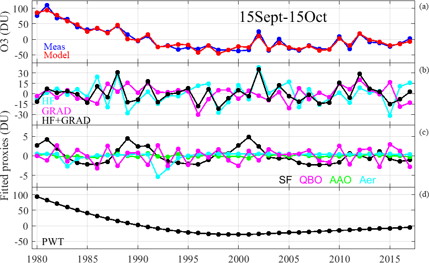
Table 3Same as Table 2 but for 15 September–15 October period. SAT dataset is also presented.
The different cases shown in Table 3 present significant trends at 2σ over the 1980–2000 and the 2001–2017 periods. The computed trend with 400–600 K range classification is comparable to the Chem-Only trend calculated by WACCM in Solomon et al. (2016). Despite the good agreement between regressed values and measurements, especially for the period of 15 September–15 October and for the range classification method (400–600 K), it is not possible to attribute ozone significant increase to ODS decrease. In addition, the ratio between trends before and after 2001 is larger than 3, which could be due to the effect of desaturation of the ozone loss.
5.2.3 Impact of GRAD proxy on trend estimation
The HF proxy represents the cumulative effect of wave activity on vortex stability (e.g. a high HF corresponds to a warmer vortex) that seems insufficient to represent total ozone variability over the last decade, especially in 2010 and 2012. The GRAD proxy was developed in order to also consider the vortex stability during both studied periods. Since Aer, QBO, SF and AAO represent lower contribution to ozone variability, trend analyses using HF, PWT proxies only and including (or not) the GRAD proxy are performed in order to highlight the impact of this parameter. Figure 10 shows residuals of MLR analysis with and without GRAD on MSR-2 data inside the vortex for the 400–600 K classification range for September and 15 September–15 October periods. The residual anomalies are significantly reduced after 2002 when GRAD is used, especially in the 15 September–15 October period. The second panels of Figs. 8 and 9 show that in some years HF and GRAD proxies are in phase, as during 2009–2014 when GRAD intensifies the HF contribution to ozone variability. This improvement is especially visible for the years 2010 and 2012. When both proxies are anticorrelated, as in 2005–2008, the improvement linked to the GRAD proxy is also observed. Tables 2 and 3 show the results of the regressions excluding GRAD proxy for September and 15 September–15 October, respectively. The determination coefficient is generally reduced by ∼ 0.07 and the χ values are 25 to 50 % larger. Trend values are mostly similar but the error bars are reduced when GRAD is used as explanatory variable, especially after 2001. Trends over the 2001–2017 period estimated without the GRAD proxy are still significant at 2σ in September and 15 September–15 October for both datasets.

Figure 10Residual (in DU) with and without contribution of GRAD proxy for September (a) and 15 September–15 October period (b).
5.2.4 PWT vs. PWLT
In order to evaluate the improvement of an additional parabolic function to the linear functions of the piece-wise trend proxy, the classical PWLT is applied in the MLR analysis of MSR-2 datasets. Figure S1 in the Supplement shows average total ozone anomalies of MSR-2 inside the vortex (400–600 K range classification method) in September and 15 September–15 October and the retrieved trends using both the PWLT and PWT methods. In the case of the 15 September–15 October period, the PWT model provides a better representation of long-term ozone evolution compared to PWLT, as it better captures ozone loss saturation during the 1990s. The trend error bars are also smaller using PWT before and after 2001. In addition, a better agreement between measurements and model values is observed with a larger R2 and lower residuals. The 2001–2017 trend error bars are ∼ 60 % larger when PWLT is used and the trend value itself is nearly double. In the case of September, a slight improvement in R2, residuals and error bars is obtained with PWT. The 2001–2017 trend value with PWLT is 40 % larger.
5.3 Results using OMD metric
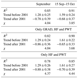
OMD has been used in previous studies to evaluate ozone loss and ozone recovery (e.g. de Laat et al., 2017). This metric has the advantage to be independent of the vortex position. Total ozone MSR-2 data were used to compute the average daily OMD on September and 15 September–15 October periods. The total ozone columns are referenced to the 220 DU threshold value and the corresponding mass deficit of the partial column (220 DU – total ozone column) is computed at each grid point (e.g. Bodeker and Scourfield, 1995). Only total ozone columns south of 60∘ S and lower than 220 DU are considered and the daily OMDs correspond to the sum of OMD at each pixel multiplied by the cosine of the latitude and the square of the Earth's radius. Table 4 shows the MLR analysis of OMD using different sets of proxies as for ozone average in Tables 2 and 3. The contributions of Aer, AAO, QBO and SF do not shown an impact on MLR analysis, where similar R2, χ, trend and error bars values are obtained. However, the inclusion of GRAD results in larger R2 and lower residuals in both periods. For the different cases and periods shown in Table 4, the OMD trend values are significant at 2σ. The MLR analysis using GRAD, HF and PWT proxies provides trends before and after 2001 of −1.29 ± 0.24 and 0.86 ± 0.36 Mt yr−1 in September and −1.61 ± 0.22 and 0.65 ± 0.33 Mt yr−1 in 15 September–15 October. De Laat el al. (2017) found a similar trend for the recovery period of 0.77 Mt yr−1 for the averaged OMD between days 220 and 280 of the year. Figure 11 displays the comparison between the OMD records and results of MLR analysis for the September and 15 September–15 October period, together with the trend components of the model. The effect of ozone loss saturation is particularly visible in the 15 September–15 October period. There are some years that are not totally explained by the model, e.g. 2002 and 2004 for both periods and 2000 for September. The contributions of GRAD, HF and GRAD + HF are shown in upper panels of Fig. S2, where GRAD intensifies HF contribution in 2010 and 2012, while both proxies are anticorrelated in 2005–2008 as observed for the total ozone analysis. The residuals with and without GRAD are shown in the bottom panels of Fig. S2. The improvement linked to the use of GRAD proxy is particularly visible in the last decade.
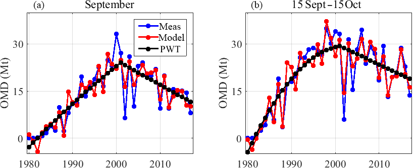
Figure 11OMD (in Mt) computed from total columns of MSR-2 dataset lower than 220 DU and south of 60∘ S for September (a) and 15 September–15 October (b). Regressed values by MLR analysis using GRAD, HF and PWT are also shown as well as the fitted PWT proxy.
Table 4Coefficient of determination R2 and trends ±2σ in Mt yr−1 before and after the turnaround year 2001 derived from multi-regression model using OMD dataset (MSR-2 total ozone columns and threshold of 220 DU; see the text) for September and 15 September–15 October over 1980–2017 period. The residual is represented in Mt by χ as explained in Table 2.
As for total ozone, MLR analysis using PWLT was performed for comparison with the PWT model. Figure S3 shows the OMD records together with PWLT and PWT components of the regression model for the both periods. Similar agreement is obtained for September but the regression results in larger residuals for 15 September–15 October using PWLT (not shown). A major difference is observed in the period 2001–2017, with a large trend value of −0.91 ± 0.41 Mt yr−1, corresponding to an increase of 40 % in absolute value.
The ozone hole is generally defined as the region with total ozone columns lower than 220 DU. This standard value was used in different studies to evaluate the ozone depletion from the OHA (e.g. Newman et al., 2006; Solomon et al., 2016) or the OMD (e.g. de Laat and van Weele, 2011; de Laat et al., 2017) metrics. In order to evaluate how the ozone hole is influenced by very low ozone values, the surface relative to the vortex area occupied by ozone values lower than different threshold levels is computed for each day and averaged over different periods (September, 15 September–15 October and October). The top panel of Fig. 12 shows the evolution of these average relative areas for five different thresholds: 220, 200, 175, 150 and 125 DU for the 15 September–15 October period. MSR-2 datasets are used for this analysis and vortex areas are estimated using the 400–600 K range classification, the results of previous sections having shown that the range classification better constrains the OHA. Results show increasing areas during the 1980s, a stabilization in the 1990s and a larger interannual variability since 2001. In contrast to the 220 DU threshold case, the evolution of relative areas corresponding to lower thresholds shows a delayed increase from the beginning of the 1980s to the early 1990s, reaching a maximum in all cases in 2000. After 2000, a larger interannual variability is generally observed and from 2006 a steady decrease is seen for thresholds lower than 200 DU. In all cases, several anomalous years are observed with important reduction of ozone depletion: 1988, 1991, 2002, 2004, 2010 and 2012. Note that these years correspond to a high contribution of HF and GRAD proxies to the regressed ozone values (Fig. 9, second panel). If we exclude these anomalous years, the 220 DU relative area remains fairly stable at about 90 % of the total vortex in average since 1990. In the most recent years, relative areas for 125 and 150 DU thresholds decrease to less than 10 and 30 %, respectively, from their peak value of 21 and 57 % reached in 2000. If such trend persists, the frequency of very low ozone values (e.g. below 125 DU) is expected to become negligible in the coming decade.
In addition, OMD were computed for the same thresholds (bottom panel of Fig. 12). The evolutions of OMD present similar behaviour as the relative area, but in this case OMD at 220 DU threshold shows a visible decrease since 2000. Nowadays OMD at a threshold lower than 150 DU presents very small values lower than 0.2 Mt.

Figure 12Relative area inside the vortex (in percent) with values lower than five level thresholds (125, 150, 175, 200 and 220 DU) computed from MSR-2 dataset using 400–600 K classification on 15 September–15 October period (a). OMD (in Mt) time series computed from MSR-2 total ozone data for the same five thresholds and time period are displayed in panel (b).
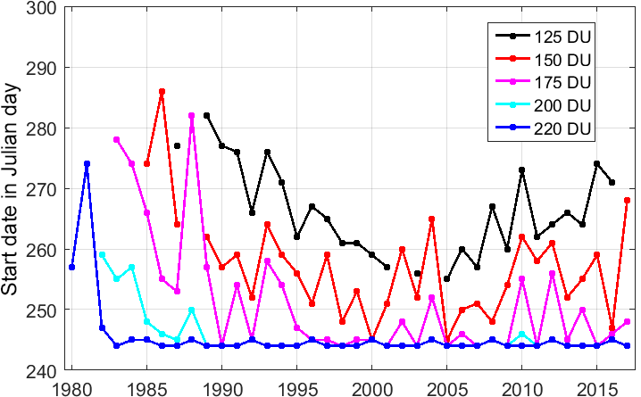
Figure 13Start day of occurrences of total ozone levels lower than different thresholds (125, 150, 175, 200 and 220 DU) computed from the MSR-2 dataset using the 400–600 K classification between 1 September and 15 October.
Solomon et al. (2016) have highlighted for the first time a delay in the formation of the ozone hole after 2000. This shift can be explained by the slower ozone loss rates after sun appearance over the pole due to ODS decrease in the polar stratosphere. In this work, such a time shift was investigated by computing the first day when ozone levels below certain thresholds occur inside the vortex (using the 400–600 K classification range), from 1 September to 15 October (Fig. 13). The same thresholds values as for Fig. 12 were used. In order to avoid influence of spurious values, the number of 1∘ × 1∘ grid cells with total ozone columns below the various thresholds in the first day (or start day) has to be larger than 10. For each curve, day values equal to 244∕245 correspond to years when ozone levels below the corresponding threshold have appeared at or before the beginning of September. For the 220 DU threshold, the dark blue curve shows that this is the case since 1983. For the 200 DU threshold, lower ozone values appear before the beginning of September after the mid-1980s. For the other thresholds, we observe a decrease, with some variability, of the start day during the 1980s, the two lowest thresholds in the 1990s and an increase after 2000–2005. This increase is most visible on the 125 DU threshold curve and to some extent also on the 150 DU threshold curve. In 2016, ozone levels below 150 DU have appeared in the beginning of September, similar to ozone holes at the end of the 1990s, but levels below 125 DU still appeared later. No values for a particular year in the threshold curves indicate that total ozone levels were above that threshold during the whole period considered. This is the case for the two lower thresholds before 1985 and for the 125 DU threshold in 2002, 2004 and 2017.
MSR-2 and SAT (TOMS and OMI with gaps in 1993–1995 filled by MSR-2) datasets have been used to evaluate total ozone trends within the southern polar vortex over the 1980–2017 period. A multi-regression model is applied to ozone values averaged over the month of September and the 15 September to 15 October period in order to compute long-term trends before and after the ODS peak in the polar stratosphere that occurred around 2001 (Newman et al., 2007). The 15 September–15 October time range corresponds to the period of maximum ozone depletion. It was not commonly used in previous works. Proxies and time windows for averaging them are selected following de Laat et al. (2015) work.
For the classification of total ozone measurements inside the vortex, the classical Nash et al. (1996) method is used. In order to evaluate the impact of vortex baroclinicity on trend analysis, classifications using a single isentropic levels (475 and 550 K) and a range of levels (400–600 K) are tested. Systematic differences are found between the various datasets. However, the interannual variability is similar, with correlation coefficients ranging from 0.98 to 0.99 in both studied periods. While larger trend values are generally found with the 475 K classification, the differences with trends related to the 400–600 K range classification are not significant at 2σ level.
The use of combined piece-wise linear and parabolic functions for the trend proxies (PWT) in the 1980–2000 and 2001–2017 periods provides a good representation of the total ozone long-term behaviour inside the vortex (after removal of interannual variability), especially for the 15 September–15 October period, probably in relation to the effect of ozone loss saturation. The classical PWLT used in previous studies seems to overestimate the trends during the recovery period.
A new proxy (GRAD) representing the vortex stability over both studied periods is included in the multilinear regression. This proxy improves the representation of total ozone interannual variability by the regressed values especially over the last decade. It results in a ∼ 0.05 larger value for the R2 determination coefficient, lower fitted residuals and smaller trend uncertainties for the different classification methods and datasets. In general, the best agreement between observations and regressed values is found for the 15 September–15 October period. While the HF combined with GRAD proxies reproduce the interannual variability of ozone quite well, other proxies such as Aer, QBO, SF and AAO present smaller explanatory power and contribute less to reduce trend uncertainties.
In the period of increasing ODSs (1980–2000), the MLR analysis shows negative and significant trends for both studied periods, similar to values found in previous studies (e.g. Kuttippurath et al., 2013, and de Laat et al., 2015). The 15 September–15 October period presents slightly larger negative trends in absolute value than the month of September.
In the 2001–2017 period, positive trends are obtained for all scenarios. The largest trends and highest significance are found for the September period, with a trend value of 1.84 ± 1 DU for the MSR-2 total ozone record using the 400–600 K range classification method. For the 15 September–15 October period, a lower trend of 1.42 ± 0.92 DU is obtained using the same record. Better fit and smaller residuals are obtained for that period. Differences with trend results from the other SAT dataset evaluated in the study are not statistically significant.
The ratio between trends before and after 2001 varies according to the studied period. Only September trends present a ratio of ∼ 3 as expected for an ozone response to ODS evolution. However, as for other trend studies based on MLR fit to observations, it is not possible from this analysis alone to fully attribute the retrieved trends to ODS evolution. For such a study, a combination of model and observations is needed. Potential feedbacks between chemistry, radiation and dynamics will play a role in ozone recovery. A recent study indicates an increase in temperatures within the vortex core from MERRA reanalyses during the period 2000–2014 in austral spring and summer (Solomon et al., 2017). Such a temperature increase that could be linked to ozone increase could play a role in the decrease of occurrence of low ozone values within the vortex and subsequent ozone increase.
The evolution of OMD was also analysed using MSR-2 data. MLR analysis on this metric confirms the findings obtained for total ozone columns, e.g. a general improvement of the fits with the GRAD proxy and the main explanatory power provided by the GRAD, HF and PWT proxies. The 2001–2017 OMD trends are larger in absolute value for September (−0.86 ± 0.36 Mt yr−1) than for 15 September–15 October (−0.65 ± 0.33 Mt yr−1). They are significant at 2σ level in both cases. These results are in general good agreement with those obtained in de Laat et al. (2017). Similar reductions of 53 and 35 % of OMD are computed for September and 15 September–15 October, respectively. This is consistent with the 30–40 % change in ODSs relative to their level in 1980, when total ozone values below the 220 DU threshold started to appear systematically (WMO, 2011).
The structural uncertainties of the MLR analysis linked to the selection of proxies were not fully analysed in this work, as in de Laat et al. (2015). The main sensitivity tests concerned the baroclinicity of the vortex and the impact of its stability during the studied periods. Trend differences in the various scenarios analysed provide some quantification of related uncertainties and are lower than the statistical trend uncertainties. Further, the large determination coefficients obtained for both periods analysed give confidence in the retrieved trends. The heat flux proxy that provides the largest explanatory power in the various fits is a well-known driver of vortex temperature conditions that are the primary causes of polar ozone depletion in periods of high ODS levels. The influence of the GRAD proxy in recent years highlights the importance of the vortex stability for the containment of the ozone hole during the period of maximum depletion.
Polar ozone recovery was also evaluated by examining the temporal evolution of relative areas occupied by ozone levels below various thresholds within the vortex. Very small total ozone columns (< 150 DU) did not occur inside the vortex before the late 1980s and early 1990s. For the 125, 150 and 175 DU thresholds, relative areas display a steady decrease since the beginning of the 21st century, while for the 200 and 220 DU thresholds, the relative area's evolution is quite stable. All relative area curves are marked by increased variability since 2000. Relative areas related to the lowest thresholds show a more rapid decrease, which further points towards polar ozone recovery. OMD records based on the same thresholds show a similar behaviour.
In summary, this work present clear symptoms of polar ozone recovery. Recovery is found for the month of September and for the first time for the period of maximum ozone depletion, e.g. from 15 September to 15 October. For both studied periods, recovery is deduced from the significant positive trends in total ozone, significant negative trends of ozone mass deficit and from the steady decrease of the occurrence of low ozone values within the polar vortex. As ODSs continue to decrease in the next years, it is likely that ozone recovery in the polar vortex in spring will become more evident.
The satellite data used to build the aerosol proxy were created by Sergey Khaykin and are available at https://drive.google.com/open?id=1lql_p0xuPpVcWVnSJhVWW6FVPTFz3ift, last access: 28 May 2018.
The supplement related to this article is available online at: https://doi.org/10.5194/acp-18-7557-2018-supplement.
The authors declare that they have no conflict of interest.
This article is part of the special issue “Quadrennial Ozone Symposium 2016 – Status and trends of atmospheric ozone (ACP/AMT inter-journal SI)”. It is a result of the Quadrennial Ozone Symposium 2016, Edinburgh, United Kingdom, 4–9 September 2016.
The authors thank NASA's GSFC and TEMIS for total ozone column data of
TOMS/SBUV/OMI-TOMS and MSR-2, respectively. They are grateful to Cathy Boone
of ESPRI data centre of Institut Pierre Simone Laplace (IPSL) for providing ERA-Interim data.
This work was supported by the Dynozpol/LEFE project funded by
the French Institut National des Sciences de l'Univers (INSU) of the Centre
National de la Recherche Scientifique (CNRS). The authors thank Susan Solomon
for fruitful interactions and the two anonymous referees
for their constructive reviews.
Edited by: Richard Eckman
Reviewed by: two anonymous referees
Allen, D., Bevilacqua, R., Nedoluha, G., Randall, C., and Manney, G.: Unusual stratospheric transport and mixing during 2002 Antarctic winter, Geophys. Res. Lett., 30, 1599, https://doi.org/10.1029/2003GL017117, 2003.
Bhartia, P. K. and Wellemeyer, C.: TOMS-V8 total O3 algorithm, in OMI Algorithm Theoretical Basis Document, vol. II, OMI Ozone Products, edited by: P. K. Bhartia, 15–31, NASA Goddard Space Flight Center, Greenbelt, Maryland, USA, 2002.
Bodeker, G. E. and Scourfield, M. W. J.: Planetary waves in total ozone and their relation to Antarctic ozone depletion, Geophys. Res. Lett., 22, 2949–2952, 1995.
Bodeker, G. E., Struthers, H., and Connor, B. J.: Dynamical containment of Antarctic ozone depletion, Geophys. Res. Lett., 29, 1098, https://doi.org/10.1029/2001GL014206, 2002.
Chipperfield, M., Bekki, S., Dhomse, S., Harris, N. R. P., Hassler, B., Hossaini, R., Steinbrecht, W., Thiéblemont, R., and Weber, M.: Detecting recovery of stratospheric ozone layer, Nature, 549, 211–218, https://doi.org/10.1038/nature23681, 2017.
Chubachi, S.: A special observation at Syowa station, Antarctica from February 1982 to January 1983, in: Atmospheric Ozone, edited by: Zerefos, C. and A. Ghazi, Springer, the Netherlands, 285–289, https://doi.org/10.1007/978-94-009-5313-0_58, 1985.
Farman, J. C., Gardiner, B. G., and Shanklin, J. D.: Large losses of total ozone in Antarctica reveal seasonal ClOx/NOx interaction, Nature, 315, 207–210, https://doi.org/10.1038/315207a0, 1985.
Dee, D. P., Uppala, S. M., Simmons, A. J., Berrisford, P., Poli, P., Kobayashi, S., Andrae, U., Balmaseda, M. A., Balsamo, G., Bauer, P., Bechtold, P., Beljaars, A. C. M., van de Berg, L., Bidlot, J., Bormann, N., Delsol, C., Dragani, R., Fuentes, M., Geer, A. J., Haimberger, L., Healy, S. B., Hersbach, H., Hólm, E. V., Isaksen, L., Kållberg, P., Köhler, M., Matricardi, M., McNally, A. P., Monge-Sanz, B. M., Morcrette, J.-J., Park, B.-K., Peubey, C., de Rosnay, P., Tavolato, C., Thépaut, J.-N., and Vitart, F.: The ERA-Interim reanalysis: configuration and performance of the data assimilation system, Q. J. R. Meteorol. Soc., 137, 553–597, https://doi.org/10.1002/qj.828, 2011.
de Laat, A. T. J. and van Weele, M.: The 2010 Antarctic ozone hole: Observed reduction in ozone destruction by minor sudden stratospheric warmings, Sci. Rep., 1, 38, https://doi.org/10.1038/srep00038, 2011.
de Laat, A. T. J., van der A, R. J., and van Weele, M.: Tracing the second stage of ozone recovery in the Antarctic ozone-hole with a “big data” approach to multivariate regressions, Atmos. Chem. Phys., 15, 79–97, https://doi.org/10.5194/acp-15-79-2015, 2015.
de Laat, A. T. J., van Weele, M., and van der A, R. J.: Onset of Stratospheric Ozone Recovery in the Antarctic Ozone Hole in Assimilated Daily Total Ozone Columns, J. Geophys. Res., 122, 11880–11899, https://doi.org/10.1002/2016JD025723, 2017.
Godin, S., Bergeret, V., Bekki, S., David, C., and Mégie, G.: Study of the interannual ozone loss and the permeability of the Antarctic polar vortex from aerosols and ozone lidar measurements in Dumont d'Urville (66.4∘ S, 140∘ E), J. Geophys. Res., 106, 1311–1330, https://doi.org/10.1029/2000JD900459, 2001.
Hauchecorne, A., Chanin, M.-L., and Keckhut, P.: Climatology and trends of the middle atmospheric temperature (33–87 km) as seen by Rayleigh lidar over the south of France, J. Geophys. Res., 96, 15297–15309, https://doi.org/10.1029/91JD01213, 1991.
Hauchecorne, A., Godin, S., Marchand, M., Heese, B., and Souprayen, C.: Estimation of the Transport of Chemical Constituents from the Polar Vortex to Middle Latitudes in the Lower Stratosphere using the High-Resolution Advection Model MIMOSA and Effective Diffusivity, J. Geophys. Res., 107, 8289, https://doi.org/10.1029/2001JD000491, 2002.
Kerzenmacher, T. E., Keckhut, P., Hauchecorne, A., and Chanin, M.-L.: Methodological uncertainties in multi-regression analyses of middle-atmospheric data series, J. Environ. Monitor., 7, 682–690, https://doi.org/10.1039/B603750J, 2006.
Khaykin, S. M., Godin-Beekmann, S., Keckhut, P., Hauchecorne, A., Jumelet, J., Vernier, J.-P., Bourassa, A., Degenstein, D. A., Rieger, L. A., Bingen, C., Vanhellemont, F., Robert, C., DeLand, M., and Bhartia, P. K.: Variability and evolution of the midlatitude stratospheric aerosol budget from 22 years of ground-based lidar and satellite observations, Atmos. Chem. Phys., 17, 1829–1845, https://doi.org/10.5194/acp-17-1829-2017, 2017.
Kuttippurath, J., Lefèvre, F., Pommereau, J.-P., Roscoe, H. K., Goutail, F., Pazmiño, A., and Shanklin, J. D.: Antarctic ozone loss in 1979–2010: first sign of ozone recovery, Atmos. Chem. Phys., 13, 1625–1635, https://doi.org/10.5194/acp-13-1625-2013, 2013.
Kuttippurath, J., Godin-Beekmann, S., Lefèvre, F., Santee, M. L., Froidevaux, L., and Hauchecorne, A.: Variability in Antarctic ozone loss in the last decade (2004–2013): high-resolution simulations compared to Aura MLS observations, Atmos. Chem. Phys., 15, 10385–10397, https://doi.org/10.5194/acp-15-10385-2015, 2015.
Levelt, P. F., van den Oord, G. H. J., Dobber, M. R., Mälkki, A., Visser, H., de Vries, J., Stammes, P., Lundell, J. O. V., and Saari, H.: The Ozone Monitoring Instrument, IEEE T. Geosci. Remote, 44, 1093–1101, 2006.
McIntyre, M. and Palmer, T.: The “surf zone” in the stratosphere, J. Atmos. Terr. Phys., 46, 825–849, https://doi.org/10.1016/0021-9169(84)90063-1, 1984.
McPeters, R., Kroon, M., Labow, G., Brinksma, E., Balis, D., Petropavlovskikh, I., Veefkind, J. P., Bhartia, P. K., and Levelt, P. F.: Validation of the Aura Ozone Monitoring Instrument total column ozone product, J. Geophys. Res., 113, D15S14, https://doi.org/10.1029/2007JD008802, 2008.
McPeters, R. D., Krueger, A. J., Bhartia, P. K., Herman, J. R., Wellemeyer, C. G., Seftor, C. J., Jaross, G., Torres, O., Moy, L., Labow, G., Byerly, W., Taylor, S. L., Swissler, T., and Cebula, R. P.: Earth Probe Total Ozone Mapping Spectrometer (TOMS) Data Products User's Guide, NASA Reference Publication 1998-206895, NASA, Washington DC, 1998.
Nair, P. J., Godin-Beekmann, S., Kuttippurath, J., Ancellet, G., Goutail, F., Pazmiño, A., Froidevaux, L., Zawodny, J. M., Evans, R. D., Wang, H. J., Anderson, J., and Pastel, M.: Ozone trends derived from the total column and vertical profiles at a northern mid-latitude station, Atmos. Chem. Phys., 13, 10373–10384, https://doi.org/10.5194/acp-13-10373-2013, 2013.
Nash, E. R., Newman, P. A., Rosenfield, J. E., and Schoeberl, M. R.: An objective determination of the polar vortex using Ertel's potential vorticity, J. Geophys. Res., 101, 9471–9478, https://doi.org/10.1029/96JD00066, 1996.
Newman, P. A., Nash, E. R., Kawa, S. R., Montzka, S. A., and Schauffler, S. M.: When will the Antarctic ozone hole recover?, Geophys. Res. Lett., 33, L12814, https://doi.org/10.1029/2005GL025232, 2006.
Newman, P. A., Daniel, J. S., Waugh, D. W., and Nash, E. R.: A new formulation of equivalent effective stratospheric chlorine (EESC), Atmos. Chem. Phys., 7, 4537–4552, https://doi.org/10.5194/acp-7-4537-2007, 2007.
Pazmiño, A. F., Godin-Beekmann, S., Ginzburg, M., Bekki, S., Hauchecorne, A., Piacentini, R., and Quel, E.: Impact of Antarctic polar vortex occurrences on total ozone and UVB radiation at southern Argentinean and Antarctic stations during 1997–2003 period, J. Geophys. Res., 110, D03103, https://doi.org/10.1029/2004JD005304, 2005.
Pazmiño, A. F., Godin-Beekmann, S., Luccini, E. A., Piacentini, R. D., Quel, E. J., and Hauchecorne, A.: Increased UV radiation due to polar ozone chemical depletion and vortex occurrences at Southern Sub-polar Latitudes in the period [1997–2005], Atmos. Chem. Phys., 8, 5339–5352, https://doi.org/10.5194/acp-8-5339-2008, 2008.
Reinsel, G. C., Weatherhead, E. C., Tiao, G. C., Miller, A. J., Nagatani, R. M., Wuebbles, D. J., and Flynn, L. E.: On detection of turnaround and recovery in trend for ozone, J. Geophys. Res., 107, 4078, https://doi.org/10.1029/2001JD000500, 2002.
Salby, M. L., Titova, E. A., and Deschamps, L.: Changes of the Antarctic ozone hole: Controlling mechanisms, seasonal predictability, and evolution, J. Geophys. Res., 117, D10111, https://doi.org/10.1029/2011JD016285, 2012.
Sato, M., Hansen, J. E., McCormick, M. P., and Pollack, J. B.: Stratospheric aerosol optical depth, 1850–1990, J. Geophys. Res., 98, 22987–22994, https://doi.org/10.1029/93JD02553, 1993.
Solomon, S., Ivy, D. J., Kinnison, D., Mills, M. J., Neely, R. R., and Schmidt, A.: Emergence of healing in the Antarctic ozone layer, Science, 353, 269–274, https://doi.org/10.1126/science.aae0061, 2016.
Solomon, S., Ivy, D., Gupta, M., Bandoro, J., Santer, B., Fu, Q., Lin, P., Garcia, R. R., Kinnison, D., and Mills, M.: Mirrored changes in Antarctic ozone and stratospheric temperature in the late 20th versus early 21st centuries, J. Geophys. Res.-Atmos., 122, 8940–8950, https://doi.org/10.1002/2017JD026719, 2017.
Steinbrecht, W., Hassler, B., Claude, H., Winkler, P., and Stolarski, R. S.: Global distribution of total ozone and lower stratospheric temperature variations, Atmos. Chem. Phys., 3, 1421–1438, https://doi.org/10.5194/acp-3-1421-2003, 2003.
van der A, R. J., Allaart, M. A. F., and Eskes, H. J.: Multi sensor reanalysis of total ozone, Atmos. Chem. Phys., 10, 11277–11294, https://doi.org/10.5194/acp-10-11277-2010, 2010.
van der A, R. J., Allaart, M. A. F., and Eskes, H. J.: Extended and refined multi sensor reanalysis of total ozone for the period 1970–2012, Atmos. Meas. Tech., 8, 3021–3035, https://doi.org/10.5194/amt-8-3021-2015, 2015.
Weber, M., Coldewey-Egbers, M., Fioletov, V. E., Frith, S. M., Wild, J. D., Burrows, J. P., Long, C. S., and Loyola, D.: Total ozone trends from 1979 to 2016 derived from five merged observational datasets – the emergence into ozone recovery, Atmos. Chem. Phys., 18, 2097–2117, https://doi.org/10.5194/acp-18-2097-2018, 2018.
WMO (World Meteorological Organization): Scientific assessment of ozone depletion: 2006, Global Ozone Research and Monitoring Project-Report 50, Geneva, Switzerland, 2007.
WMO (World Meteorological Organisation): Scientific assessment of ozone depletion: 2010, Global Ozone Research and Monitoring Project, Report 52, Geneva, Switzerland, 516 pp., 2011.
WMO (World Meteorological Organization): Scientific Assessment of Ozone Depletion: 2014, Global Ozone Research and Monitoring Project, Report No. 55, Geneva, Switzerland, 416 pp., 2014.
Yang, E.-S., Cunnold, D. M., Newchurch, M. J., Salawitch, R. J., McCormick, M. P., Russell, J. M., Zawodny, J. M., and Oltmans, S. J.: First stage of Antarctic ozone recovery, J. Geophys. Res., 113, D20308, https://doi.org/10.1029/2007JD009675, 2008.
- Abstract
- Introduction
- Total ozone column data series
- Data classification within the vortex
- Vortex baroclinicity
- Trend analysis
- Temporal evolution of low total ozone values inside the vortex
- Conclusions
- Data availability
- Competing interests
- Special issue statement
- Acknowledgements
- References
- Supplement