Convective environment in pre-monsoon and monsoon conditions over the Indian subcontinent: the impact of surface forcing

Thermodynamic soundings for pre-monsoon and monsoon seasons from the Indian subcontinent are analysed to document differences between convective environments. The pre-monsoon environment features more variability for both near-surface moisture and free-tropospheric temperature and moisture profiles. As a result, the level of neutral buoyancy (LNB) and pseudo-adiabatic convective available potential energy (CAPE) vary more for the pre-monsoon environment. Pre-monsoon soundings also feature higher lifting condensation levels (LCLs). LCL heights are shown to depend on the availability of surface moisture, with low LCLs corresponding to high surface humidity, arguably because of the availability of soil moisture. A simple theoretical argument is developed and showed to mimic the observed relationship between LCLs and surface moisture. We argue that the key element is the partitioning of surface energy flux into its sensible and latent components, that is, the surface Bowen ratio, and the way the Bowen ratio affects surface buoyancy flux. We support our argument with observations of changes in the Bowen ratio and LCL height around the monsoon onset, and with idealized simulations of cloud fields driven by surface heat fluxes with different Bowen ratios.

1 Introduction

The convective environment over the Indian subcontinent changes significantly from hot and dry pre-monsoon conditions to cooler and wetter monsoon conditions. The change comes from the dramatic evolution of the large-scale circulation (e.g. Yin, 1949 and Lau and Yang, 1996, and references therein) that brings significant oceanic moisture during the monsoon. The conveyer belt of moisture is the monsoon low-level jet (Joseph and Sijikumar, 2004) that moistens land areas, changes cloud characteristics, and brings monsoon rains that are key to the Indian economy. The change from pre-monsoon to monsoon conditions is rapid, with convective precipitation driven by the surface heating in the pre-monsoon period giving way to an increase in cloud cover and surface rainfall during the monsoon season (e.g. Ananthakrishnan and Soman, 1988). Significant rainfall occurs over the west coast and the north-eastern region, and it further extends westward in association with the north-westward movement of weather systems formed over the Bay of Bengal (Gadgil et al., 1984).

The monsoon low-level jet weakens during the monsoon break periods, influencing moisture content over land and strongly reducing the rainfall (Sandeep et al., 2014; Balaji et al., 2017). Intraseasonal oscillations of monsoon rainfall are well documented (e.g. Goswami and Mohan, 2001; Gadgil, 2003), with active and break periods featuring considerable spatio-temporal variations (Rajeevan et al., 2010). Initial studies of the monsoon boundary layers (BLs) focused on the contrast between active and break monsoon periods (e.g. Parasnis et al., 1985), with a contrasting moisture availability in the lower troposphere. The active/break monsoon conditions are characterized by lower/higher boundary layer heights (e.g. Kusuma et al., 1991). Higher cloud bases also occur during weak monsoon conditions when the lower atmosphere is drier compared to the active monsoon. Parasnis and Goyal (1990) report enhanced convective instability in the boundary layer on weak monsoon days when compared to the active monsoon. Convective available potential energy (CAPE), a proxy for the strength of convection, feature higher values over coastal regions because of the presence of more moisture in the boundary layer (Alappattu and Kunhikrishnan, 2009). That study argues that the temporal variability of CAPE and convective inhibition is predominantly controlled by the BL moisture. Resmi et al. (2016) show that sustaining convective storms in the diurnal cycle is possible because of moisture advection and increase of CAPE over the rain shadow region of the Indian subcontinent. Diurnal variations of CAPE are directly linked to water vapour content near the surface, with higher CAPE environments favouring higher precipitation (Balaji et al., 2017). Precipitable water (PW) and lifting condensation level (LCL) derived from various observations are also closely related (Murugavel et al., 2016). Balaji et al. (2017) show that high PW conditions correspond to a shallower boundary layer (with a boundary layer height close to the LCL) and a higher LCL combined, with a deeper boundary layer height typically occurring during drier conditions. Balaji et al. (2017) also illustrate diurnal variations of PW and CAPE during wet and dry regimes within the monsoon.

The monsoon onset marks a striking change in the surface and boundary layer conditions because of the change of the partitioning of the surface energy flux into its sensible and latent components. However, there are no comprehensive comparisons of pre-monsoon and monsoon thermodynamic environments and their contrasting characteristics with respect to parcel buoyancy and boundary layer characteristics. The soil moisture variations typically follow rainfall patterns or variations. Transition from pre-monsoon to monsoon conditions is associated with an increase in soil moisture (Sathyanadh et al., 2016) and thus with the change of the partitioning of the surface energy flux into its sensible and latent fluxes. The ratio of the sensible to latent surface heat fluxes is commonly referred to as the Bowen ratio. The Bowen ratio affects the surface buoyancy flux that drives boundary layer dynamics (e.g. Stevens, 2007, and references therein) and affects the rate at which the convective boundary layer deepens. It also sets the mean boundary layer humidity (e.g. Ek and Mahrt, 1994) and impacts the efficiency of the moist convection heat cycle (i.e. the ratio between mechanical work and energy input at the surface; Shutts and Gray, 1999) and the distribution of the shallow convection cloud base mass flux (Sakradzija and Hohenegger, 2017). One might thus expect different boundary layer characteristics in surface-forced pre-monsoon and monsoon conditions due to different Bowen ratios for the two environments. However, the Bowen ratio does not seem to affect the updraft intensity in deep convection (Hansen and Back, 2015). Instead, the free-tropospheric conditions, impacted by larger scale atmospheric dynamics, may affect the strength of convection as measured by parameters such as CAPE, LCL height, or maximum pseudo-adiabatic parcel buoyancy.

The present study contrasts pre-monsoon and monsoon environments by analysing a large set of soundings released from Pune, India, in the semi-arid Western Ghat mountains rain shadow region. Traditional measures of the convective environment are discussed, with the emphasis on surface forcing. Since no surface flux information is available for the region where long period soundings were obtained, we use data collected at another location in the rain shadow area to document changes in the Bowen ratio and LCL height between pre-monsoon and monsoon conditions. Subsequently, we discuss two sets of idealized numerical simulations that consider the impact of the surface Bowen ratio on convective development. We argue that model results are broadly consistent with our interpretation of the sounding analysis. A brief summary concludes the paper.

2 Observations

2.1 Data and instrumentation

Data from radiosonde measurements conducted at Pune (18^∘31^′ N, 73^∘51^′ E; elevation 530 m a.m.s.l.) and measurements from Mahabubnagar (16^∘45^′ N, 78^∘00^′ E; elevation 498 m a.m.s.l.), about 500 km south-east of Pune) are used in this study. Both locations are in the lee side of the Western Ghat mountains in the semi-arid rain shadow region. A total of 84 soundings from the years 2010 to 2014 from Pune, divided into 42 pre-monsoon (March, April, May) and 42 monsoon (June, July, August, September) soundings, were analysed. The Pune soundings are launched irregularly (typically once a week) and they are not part of the daily global sounding network (i.e. they are not available, for instance, from the Wyoming air sounding database; http://weather.uwyo.edu/upperair/sounding.html, last access: 1 July 2016). The original data are archived at the Indian Institute for Tropical Meteorology (IITM) and they feature a high spatial resolution as explained below. The Vaisala radiosonde RS92-SGP is used, measuring atmospheric temperature, pressure, and humidity. Wind speed and direction (not considered in this study) are obtained by tracking the position of the radiosonde using GPS. The launch time is 13:00 IST when the solar insolation is near its peak. The operation takes almost 2 h, with the radiosonde typically reaching up to 30 km altitude, with an ascent rate of around 5 m s⁻¹. Data are available at approximately 3 m vertical resolution.

The second set of observations are surface flux and tropospheric profiles from the Integrated Ground Observational Campaign (IGOC) at Mahabubnagar, south-east of Pune. Observations were conducted during the transition from pre-monsoon to monsoon and during the monsoon season of 2011. The latent and sensible surface heat fluxes were measured using eddy covariance sensors located on a meteorological tower at 6 m above surface. In addition to the surface heat flux measurements, a microwave radiometer profiler (MWRP) was also placed about 1.2 km from the tower location. The MWRP provides vertical profiles of temperature and humidity during the diurnal cycle (Balaji et al., 2017). This information is used to calculate the lifting condensation level, applying the same method as for the Pune soundings (see the next section).

2.2 Analysis of Pune soundings

For Pune soundings, thermodynamic parameters, such as the potential temperature (θ), equivalent potential temperature (θ_e), water vapour mixing ratio (q_v), relative humidity (RH), cloud water mixing ratio (q_c), parcel buoyancy (B), and cumulative convective available potential energy (cCAPE), were derived using thermodynamic equations and standard procedures as described below. Standard parameters describing the convective environment, such as the lifting condensation level (LCL), the level of free convection (LFC), and the level of neutral buoyancy (LNB), were calculated as well.

Pressure (p), temperature (T), q_v, and RH of the environment were given as the standard sounding data. Geometrical heights of data levels were obtained by integrating the hydrostatic pressure equation from the surface upwards. Subsequently, the input data were interpolated to a regular vertical grid with a uniform spacing of 50 m. A simple adiabatic parcel model was then applied to calculate various parameters describing convective environment. Initial conditions for the parcel came from the lowest levels available in the sounding, typically corresponding to the near-surface conditions. The θ, q_v, q_c, and the B inside the parcel (i.e. neglecting cloud water which is assumed to convert to precipitation and fall out) were derived, considering only condensation of water vapour. Condensation was calculated, assuming that the parcel maintained water saturation, and the corresponding latent heating was added to the parcel potential temperature. The first level where condensation occurred was marked as LCL. The level above LCL where parcel buoyancy became positive was marked as LFC, and the level where parcel buoyancy changed from positive to negative (typically in the upper troposphere) was marked as LNB. Pseudo-adiabatic parcel buoyancy was calculated as $B=g(\mathrm{\Delta }{\mathit{\theta }}_{\mathrm{v}}/{\mathit{\theta }}_{\mathrm{ve}})$, where θ_v and θ_ve are virtual potential temperatures of the rising parcel and of the environment, respectively, and g is gravitational acceleration. The virtual potential temperature is defined as ${\mathit{\theta }}_{\mathrm{v}}=\mathit{\theta }(\mathrm{1}+\mathit{\epsilon }{q}_{\mathrm{v}})$, where $\mathit{\epsilon }=R_{\mathrm{v}}/R_{\mathrm{d}}-\mathrm{1}\approx \mathrm{0.61}$ and R_v and R_d are gas constants for the water vapour and dry air, respectively. The cCAPE was calculated by vertical integration of the parcel positive buoyancy; it is formally defined as $\text{cCAPE}\left(z\right)={\int }_{\mathrm{0}}^{z}max(\mathrm{0},B)\mathrm{d}z$. Cumulative CAPE shows how CAPE builds up within a rising pseudo-adiabatic parcel. Note that CAPE is given as cCAPE(z=LNB). In addition, the equivalent potential temperature θ_e was calculated using the following approximate formula:

$$\begin{array}{}\text{(1)}& {\mathit{\theta }}_{\mathrm{e}}=\mathit{\theta }\exp \left({\displaystyle \frac{L}{C_{\mathrm{p}}T}}{q}_{\mathrm{v}}\right),\end{array}$$

where L is the latent heat of condensation.

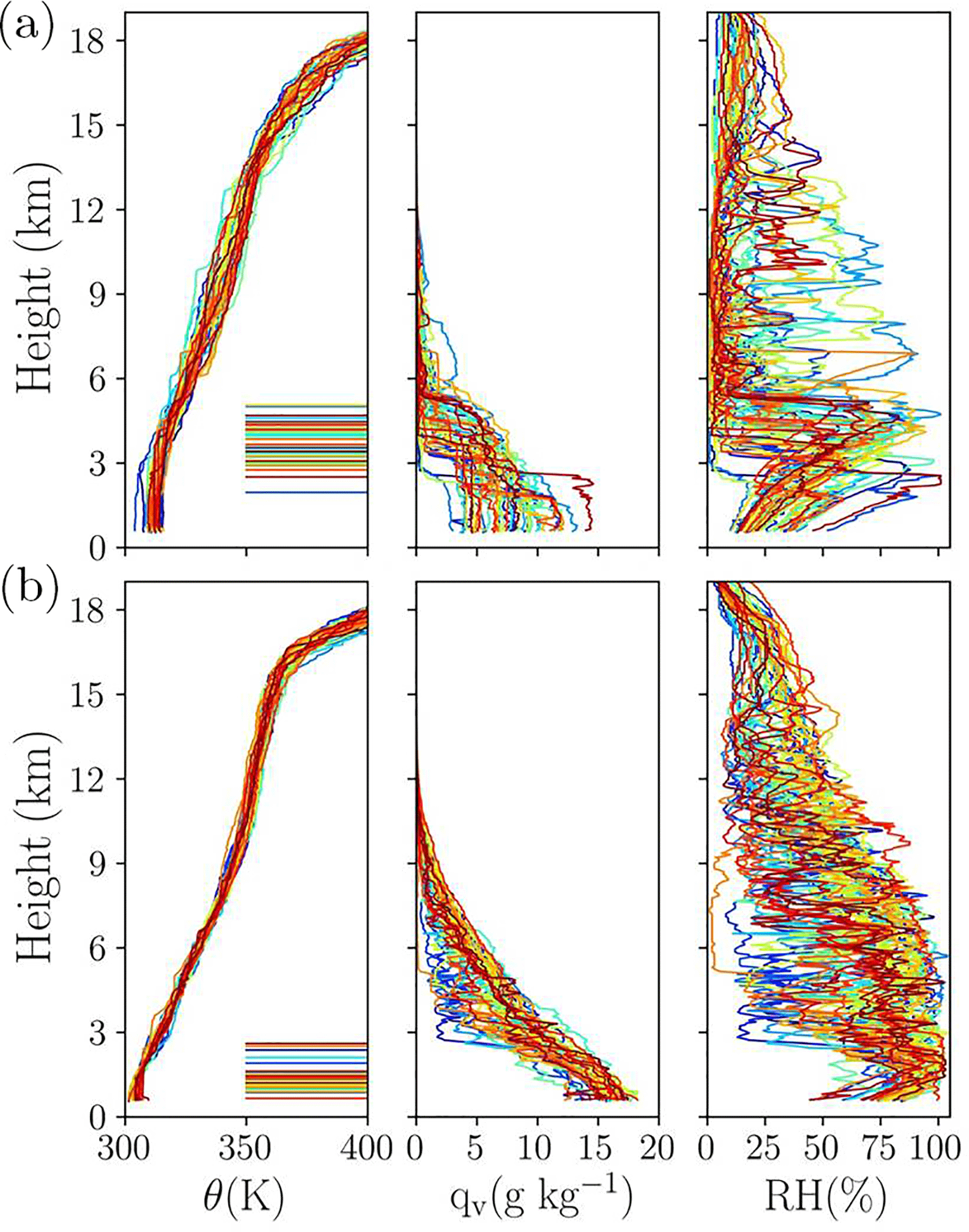
Figure 1 Profiles of potential temperature (θ), water vapour mixing ratio (q_v), and relative humidity (RH) for (a) pre-monsoon and (b) monsoon soundings. Different colours represent different soundings, with a total of 42 soundings for both cases. The horizontal lines in the left-hand panels are LCL heights, with the same colours as the corresponding profile.

3 Results of sounding analysis

3.1 Temperature and moisture profiles

Figure 1 shows vertical profiles of θ, q_v, and corresponding RH, separated into pre-monsoon and monsoon periods. Panels with the potential temperature profiles also show corresponding LCLs, represented by horizontal lines. The atmosphere exhibits contrasting features during the two seasons. Pre-monsoon soundings are characterized by a deeper BL than monsoon soundings. The BL can be identified by regions of constant potential temperature in the lower atmosphere up to 3 km from the surface. LCL heights show higher cloud base heights for pre-monsoon clouds and lower cloud base heights for monsoon clouds. The lower and middle troposphere is significantly more humid for the monsoon when compared to the pre-monsoon. The pre-monsoon BL is typically topped by a strong inversion that is accompanied by a decrease of RH within a few hundred metres. Higher RH for the monsoon BL, with values closer to saturation, is evident. Monsoon soundings show a well-defined tropopause identified from the potential temperature sharp gradient at the height of around 16 km. Details of these are discussed in Sect. 3.1.1–3.1.3.

3.1.1 Temperature and moisture profiles and their variability

For pre-monsoon conditions, the surface temperature is on average several degrees warmer and water vapour mixing ratio is on average about half of that of the monsoon period. The latter is arguably related to the contrasting levels of soil moisture in pre-monsoon and monsoon conditions. The temperature and moisture profiles exhibit less day-to-day variability for the monsoon period. The spread of temperature in the middle troposphere in the monsoon environment is about half of that for the pre-monsoon. In the upper troposphere and the lower stratosphere, the differences are smaller. For the pre-monsoon period, moisture profiles below 6 km vary significantly and the atmosphere is significantly drier above 6 km when compared to monsoon soundings. Arguably, higher moisture contents in the middle and upper troposphere during the monsoon come from convection reaching higher levels as documented later in the paper. However, differences due to large-scale horizontal advection may play some role as well.

Individual moisture profiles feature significant fluctuations, which are even more apparent if no smoothing is applied to the original high-resolution data. This is evident at lower levels (i.e. within the boundary layer) as well as aloft. Fluctuations within the boundary layer show that it is not well mixed for the water vapour in most soundings, especially for monsoon conditions. However, relative humidity does increase approximately linearly within the boundary layer in most profiles similar to the case of the well-mixed boundary layer (i.e. featuring a constant with the height potential temperature and water vapour mixing ratio).

3.1.2 LCL/boundary layer height

In surface-driven convective situations and midday conditions with either shallow or deep convective clouds above the boundary layer, LCL height should be relatively close to boundary layer height, as noted by Balaji et al. (2017) using temperature and moisture profile observations with a microwave radiometer profiler. This is because the adiabatic (neutral) temperature profile (i.e. constant θ) within the well-mixed boundary layer has to change to a stably stratified profile (i.e. θ increasing with height) in the free troposphere aloft. Since the LCL marks the transition from a dry to a moist temperature lapse rate within a rising adiabatic parcel, the change from a neutral boundary layer and moist-convecting stratified atmosphere aloft should also correspond to the LCL. This is consistent with idealized simulations of the diurnal cycle of shallow and deep convection over land (see Brown et al., 2002, and Grabowski et al., 2006, respectively). These simulations show that a deepening of boundary layer is accompanied by an increase of LCL height. However, the presence of deep convection and significant precipitation can lead to the separation of the well-mixed boundary layer height and LCL height, as illustrated later in the paper in idealized simulations (cf., Sect. 5). As Fig. 1 documents, LCLs around 13:00 LST (local sidereal time) are significantly higher for the pre-monsoon period. This may come from either different surface fluxes during the course of the day between pre-monsoon and monsoon periods or from partitioning of the surface energy flux into sensible and latent components. One can argue, however, that the energy that passed from the earth surface to the atmosphere (the sum of sensible and latent heat fluxes) should be similar in pre-monsoon and monsoon conditions because the solar insolation is similar in both cases. The presence of extensive clouds in monsoon conditions can make a difference to the surface energy budget, but we neglect this aspect for the qualitative discussion here. Thus, we assume that development of the convective boundary layer during pre-monsoon and monsoon periods is, to the leading order, affected by partitioning of total surface energy flux into its sensible and latent components, and not by the differences in total flux.

The partitioning of the surface flux into sensible and latent components depends on the soil moisture that differs drastically between pre-monsoon and monsoon conditions. The surface buoyancy flux that drives boundary layer dynamics is affected by the surface Bowen ratio. Since the thermodynamic variable relevant for the buoyancy flux is the virtual potential temperature ${\mathit{\theta }}_{\mathrm{v}}=\mathit{\theta }(\mathrm{1}+\mathit{\epsilon }{q}_{\mathrm{v}})$, the total surface buoyancy flux (BF) can be approximated as $\text{BF}=<w{\mathit{\theta }}_{\mathrm{v}}\mathit{>=}<w\mathit{\theta }>+{\mathit{\theta }}_{\mathrm{o}}\mathit{\epsilon }<w{q}_{\mathrm{v}}>$, where θ_o is the surface potential temperature. The total surface energy flux (EF) can be similarly written (using the moist static energy or the equivalent potential temperature) as $\text{EF}=<w\mathit{\theta }>+\frac{L}{c_{\mathrm{p}}}<w{q}_{\mathrm{v}}>$. Consequently, the BF / EF ratio between the buoyancy and energy surface fluxes can then be represented as

$$\begin{array}{}\text{(2)}& \text{BF}/\text{EF}=(\mathit{\alpha }+B)/(\mathrm{1}+B),\end{array}$$

where $\mathit{\alpha }={\mathit{\theta }}_{\mathrm{o}}\mathit{\epsilon }\frac{c_{\mathrm{p}}}{L}\approx \mathrm{0.1}$ is a numerical coefficient, and $B=\frac{c_{\mathrm{p}}<w\mathit{\theta }>}{L<w{q}_{\mathrm{v}}>}$ is the Bowen ratio. For small Bowen ratios (i.e. the surface latent heat flux dominates as typically over the oceans), the BF ∕ EF ratio approaches 0.1; that is, only 10 % of the total surface energy flux contributes to the buoyancy flux. For large Bowen ratios (i.e. the surface sensible heat flux dominates as over arid and semi-arid areas) the BF ∕ EF ratio approaches 1; that is, all of the total surface energy flux contributes to the buoyancy flux. For a Bowen ratio of 1 (i.e. equal surface sensible and latent fluxes), only about half of the energy flux contributes to the buoyancy flux. Equation (2) is shown in Fig. 2. The impact of the surface Bowen ratio on the shallow convective cloud base mass flux has recently been highlighted by Sakradzija and Hohenegger (2017).

The above considerations explain the well-known fact that the daytime convective boundary layer deepens over arid and semi-arid areas that feature a high Bowen ratio due to limited availability of water at the surface. For instance, over the Sahara desert, the boundary layer height can reach several kilometres (e.g. Ao et al., 2012). In contrast, the surface-driven convective boundary layer over tropical and subtropical oceans is relatively shallow, often a mere several hundred metres. We argue that the differences between pre-monsoon and monsoon periods can, to a large degree, be explained by the availability of soil moisture and partitioning of surface energy flux between sensible and latent components. These differences will be further illustrated by model simulations discussed in Sect. 5.

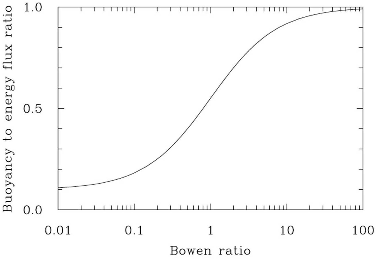
Figure 2 The ratio of the surface buoyancy flux to the total energy flux (sensible plus latent) as a function of the Bowen ratio.

3.1.3 Troposphere–stratosphere transition

As Fig. 1 illustrates, the tropopause is much better defined and varies less during monsoon. In contrast, transition from the troposphere to the stratosphere is gradual in the pre-monsoon environment. This may come from the fact that convection does not always have a chance to get to the tropopause in the pre-monsoon environment (as documented later in the paper) and other processes (e.g. large-scale advection or radiative transfer) play an important or even dominant role. A well-defined tropopause is a feature of the monsoon environment. This is associated with the mid-tropospheric anticyclone of the Asian monsoon system. Dethof et al. (1999) show that the upper-level monsoon anticyclone located close to the tropopause is moistened by the monsoon convection. The strong potential vorticity gradients around the tropopause prevent transport across the upper troposphere–lower stratosphere (UTLS) region and result in strong temperature gradients there. The latitude of Pune is in the region that separates upper-level westerlies to the north and easterlies to the south, which are associated with mid-tropospheric anticyclone.

In the case of pre-monsoon conditions, the moisture availability in BL is considerably reduced and this has a significant influence on the cloud base height. Air parcels need to rise to greater heights in pre-monsoon conditions to reach the LCL compared to monsoon conditions. Significant variations are observed in LCL heights during these two seasons. Pre-monsoon clouds have their bases at higher levels, 2 to 6 km from the surface, whereas monsoon soundings indicate cloud bases at lower levels, with most of them being lower than 2 km. This result is highly correlated with surface-level moisture as documented below.

The BL as well as the mid-tropospheric moisture for the two seasons exhibit contrasting characteristics. The mean tropospheric moisture is higher for monsoon soundings. During the monsoon, the surface values of q_v are higher compared to the pre-monsoon, and most of them fall within the range of 14–18 g kg⁻¹. Pre-monsoon surface q_v has a lower but wider range from 3 to 14 g kg⁻¹. Monsoon soundings also indicate higher levels of mid-tropospheric moisture. The main reason is south-westerly winds that transport moisture from the Arabian Sea to the Indian subcontinent. Because of the Western Ghat mountains, the transport features strong low-level convergence over the Indian west coast. However, for the inland locations over the rain shadow region, the jet core level is seen at 1.5–2 km, just above the boundary layer. Arguably, boundary layer convection developing during the day pushes the jet layer to an elevated height.

3.2 Cloud base height and surface-level moisture

For a well-mixed boundary layer, the water vapour mixing ratio near the surface is the main determining factor for the cloud base height. Figure 3 shows the scatter plot of the cloud base height and the surface moisture. Monsoon soundings with higher surface mixing ratios correspond to lower cloud bases, and pre-monsoon soundings with lower mixing ratios have significantly higher cloud bases. The relationship between the mixing ratio at the surface and the cloud base height is approximately linear but with a significant scatter. However, the relationship between cloud base height and near-surface RH is non-linear, with little scatter.

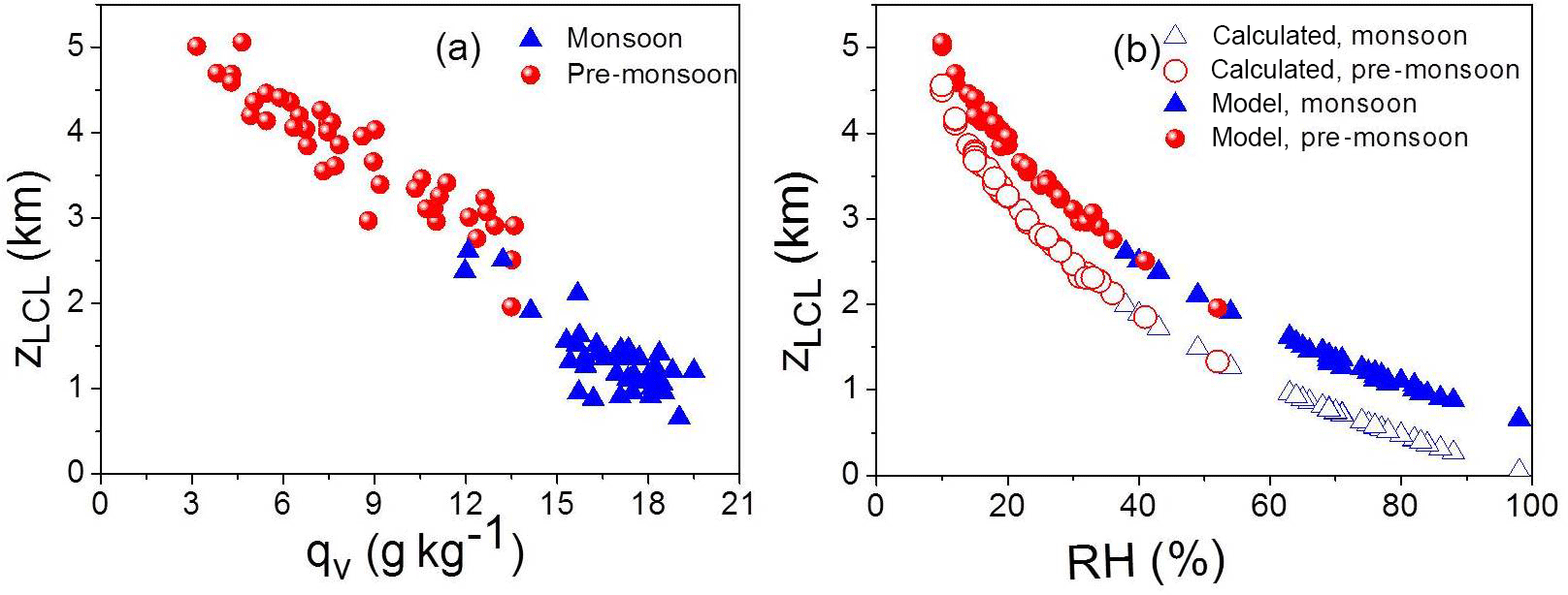
Figure 3 Variation of LCL height z_LCL with (a) surface q_v and (b) surface RH. Red/blue circles/triangles represent pre-monsoon/monsoon cases. Parcel-model-derived parameters (RH and LCL height) are shown as filled symbols. LCL heights derived using Eq. (3) are shown as empty symbols.

The following simple theoretical analysis explains the close relationship between the surface relative humidity and the cloud base height as shown in Fig. 3. The key assumptions are that the boundary layer is well mixed and the cloud base is not far from the boundary layer top. The two assumptions ensure that air parcels originating from near the surface and reaching the LCL insignificantly change their thermodynamic properties during their rise. Overall, these should be valid assumptions in surface-driven convective situations. However, the presence of significant precipitation can change this picture, as documented later in the paper. When the two assumptions are valid, then the height of the cloud base (i.e. LCL) is the level where the adiabatic air parcel rising from surface reaches saturation. If T_LCL depicts the LCL temperature and T_s and RH_s depict temperature and relative humidity at the surface, then $q_{\mathrm{vs}}\left(T_{\mathrm{LCL}}\right)/q_{\mathrm{vs}}\left(T_{\mathrm{s}}\right)={\text{RH}}_{\mathrm{s}}$. Since $q_{\mathrm{vs}}\approx e_{\mathrm{s}}/p$, where e_s and p are the saturation water vapour pressure and environmental air pressure, it follows that $e_{\mathrm{s}}\left(T_{\mathrm{LCL}}\right)/e_{\mathrm{s}}\left(T_{\mathrm{s}}\right)=p_{\mathrm{LCL}}/p_{\mathrm{s}}{\text{RH}}_{\mathrm{s}}$, where p_LCL and p_s represent pressure at the LCL and the surface, respectively. Applying an approximate Clausius–Clapeyron formula in the form $e_{\mathrm{s}}\left(T\right)=e_{\mathrm{0}}\exp \left[\frac{L}{R_{\mathrm{v}}}\left(\frac{\mathrm{1}}{T_{\mathrm{0}}}-\frac{\mathrm{1}}{T}\right)\right]$, where e₀ is the saturated water vapour pressure at the temperature T₀, leads to $\frac{\mathrm{1}}{T_{\mathrm{s}}}-\frac{\mathrm{1}}{T_{\mathrm{LCL}}}=\frac{R_{\mathrm{v}}}{L}\ln \left(\frac{p_{\mathrm{LCL}}}{p_{\mathrm{s}}{\text{RH}}_{\mathrm{s}}}\right)$. Using the dry adiabatic relationship between T_LCL and T_s in the form $T_{\mathrm{LCL}}=T_{\mathrm{s}}-\frac{g{z}_{\mathrm{LCL}}}{C_{\mathrm{p}}}$ gives

$$\begin{array}{}\text{(3)}& \ln \left({\displaystyle \frac{p_{\mathrm{LCL}}}{p_{\mathrm{s}}{\text{RH}}_{\mathrm{s}}}}\right)=-{\displaystyle \frac{Lg{z}_{\mathrm{LCL}}}{c_{\mathrm{p}}{R}_{\mathrm{v}}{T}_{\mathrm{LCL}}{T}_{\mathrm{s}}}}.\end{array}$$

To show that the relationship is approximately valid for the data used in this study, we derived z_LCL from observed p_s, RH_s, and T_s, and the parcel model derived p_LCL and T_LCL. As the figure shows, Eq. (3) provides z_LCL estimates that are lower than the z_LCL calculated from the parcel model, and the difference between z_LCL estimated from the parcel model and derived from Eq. (3) is typically around 600 m, regardless of the surface humidity.

There are at least two explanations for the underestimation of z_LCL by Eq. (3), both associated with the well-mixed assumption for the boundary layer. The first one has to do with the presence of superadiabatic layer near the surface (i.e. the potential temperature decreasing with height), clearly evident in many soundings shown in Fig. 1. With the surface temperature higher than the mean boundary layer potential temperature, z_LCL needs to be higher to keep z_LCL/(T_LCLT_S) approximately constant on the right-hand side of Eq. (3) as p_LCL∕p_s can change little. Since 600 m corresponds to about 6 K along the dry adiabatic lapse rate, such an explanation would imply that the air temperature change across the superadiabatic layer is universally about 6 K in the sounding data used here. This does not seem inconsistent with at least some soundings shown in Fig. 1. The boundary layer may also become not well mixed (i.e. develop moisture and temperature stratification) because of precipitation or low-level horizontal advection; the presence of neither is possible to deduce from the available data. In convective situations, significant surface precipitation is always accompanied by convective-scale downdrafts and BL cold pools. Since the air in a cold pool typically comes from the middle troposphere, the low-level water vapour mixing ratio inside the cold pool is typically lower than on the outside (e.g. Tompkins, 2001). In such a situation, the boundary layer cannot be assumed to be well mixed and entrainment of the BL air into a plume rising from surface would lead to plume dilution and thus to the increase of LCL height. Moreover the parcel model constitutes a significant simplification of the real atmosphere in which the sonde is flown, taking a Lagrangian path and cutting across different air columns.

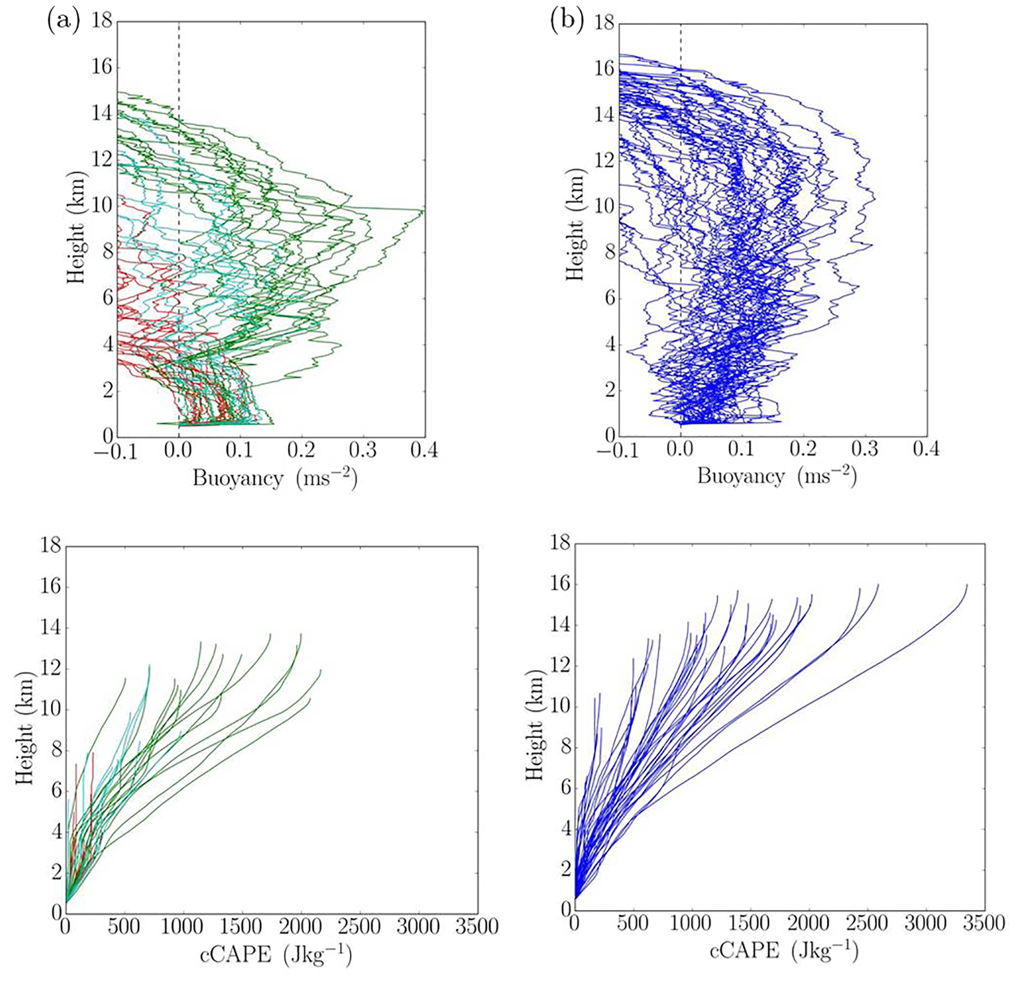
Figure 4 Profiles of the pseudo-adiabatic buoyancy (upper panels) and cCAPE (lower panels) for pre-monsoon (a) and monsoon (b) soundings. cCAPE profiles terminate at LNB. Pre-monsoon soundings are divided into three groups marked by red, light blue, and green lines, depending on the CAPE value.

The above analysis is consistent with results discussed in Murugavel et al. (2016). They showed that the column precipitable water (PW), the vertical integral of water vapour density in the atmosphere, is a good predictor of LCL temperature and height over the Indian subcontinent. Since the column PW is dominated by moisture in the lowest levels (and in the boundary layer in particular), the mixing ratio near the surface should then be well correlated with LCL height, as documented in Fig. 3.

The above results can also be used in reverse. The fact that, despite some offset, there is an almost a perfect relationship between RH and z_LCL implies that the midday boundary layer for all soundings considered in this study is of a convective type, that is, with close to the adiabatic potential temperature profile from above the superadiabatic surface layer up to the convective boundary layer height and the LCL.

3.3 Profiles of pseudo-adiabatic buoyancy and cCAPE

CAPE represents the energy available for moist convection, and larger values of CAPE indicate a larger potential for strong convection. Figure 4 shows profiles of pseudo-adiabatic buoyancy (i.e. the difference in the virtual potential temperature between the pseudo-adiabatic parcel and the environment) and cCAPE from all soundings separated into pre-monsoon and monsoon conditions. In addition, pre-monsoon soundings are divided into three groups (marked by red, blue, and green lines in the left-hand panels) depending on CAPE values, with red/blue/green colours corresponding to low/medium/high CAPE values. This partitioning will be used in the subsequent analysis. Monsoon and pre-monsoon environments exhibit distinct patterns. First, there is a significant day-to-day variability for both environments as marked by the spread in profiles, but the variability seems larger for pre-monsoon conditions. The variability is affected mostly by the surface water vapour mixing ratio, as quantified later in the paper. Large CAPE pre-monsoon soundings (green colour) are characterized by pseudo-adiabatic parcel maximum buoyancies that are not different from their monsoon counterparts, but LNBs and CAPE values (evident from end points of cCAPE profiles) are typically lower for the pre-monsoon environment.

Most of the monsoon pseudo-adiabatic buoyancy and cCAPE profiles follow a consistent pattern, as shown in the right-hand panels of Fig. 4. These soundings maintain positive pseudo-adiabatic buoyancies up to the upper troposphere, with CAPE values typically between 1000 and 2000 J kg⁻¹, except for a few cases. This is different for pre-monsoon soundings that feature a wide range of maximum in-cloud buoyancies, with three distinct branches. The first branch represented by green lines follows a pattern similar to monsoon cases, but with lower CAPE values and lower LNBs. The second branch, marked by blue lines, represents intermediate soundings, with CAPE typically between 500 and 1000 J kg⁻¹, and LNBs typically in the middle troposphere. Red lines represent the cases with low CAPE and LNBs located in the lower or middle troposphere.

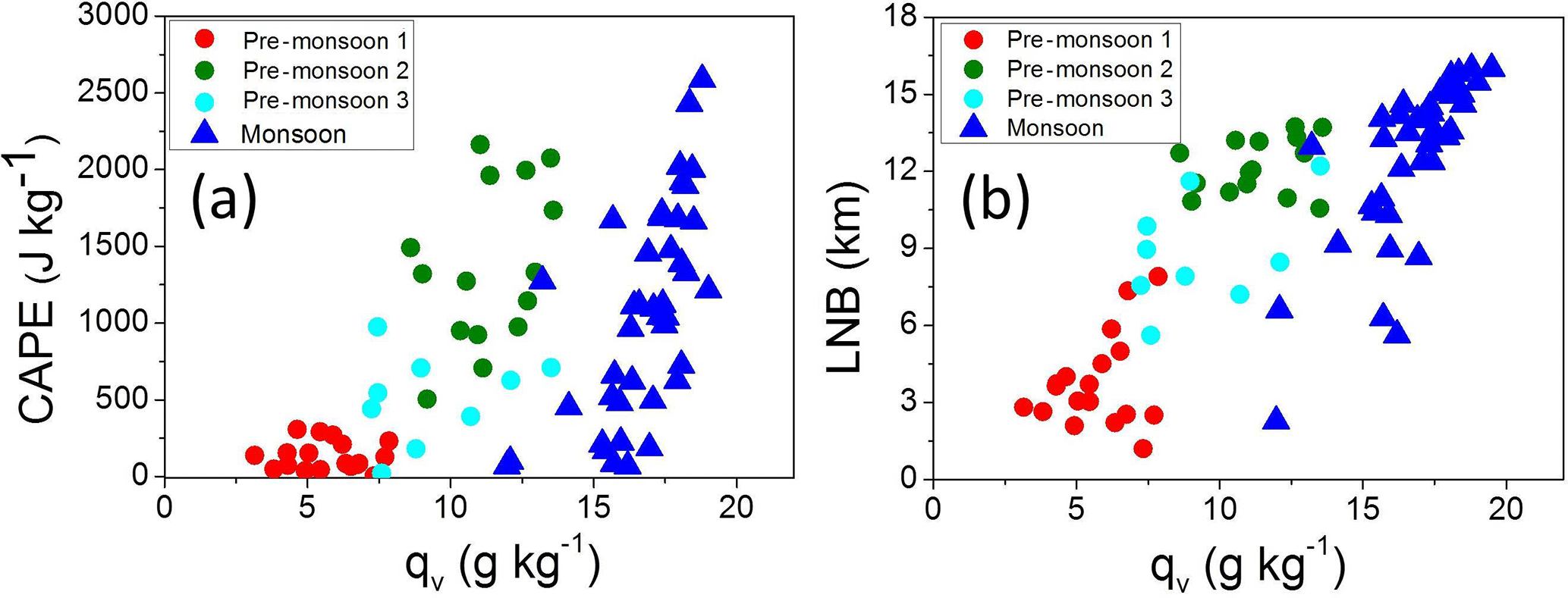
Figure 5 Variation of (a) CAPE and (b) LNB as a function of the surface water vapour mixing ratio. Pre-monsoon cases are grouped similarly as in Fig. 4.

These results show that the monsoon season features convective environments that are all similar and can be grouped into a single family. In contrast, the pre-monsoon season witnesses a wide range of atmospheric conditions and convection with diverse properties, from situations with low CAPE and LNBs in the lower and middle troposphere to situations with CAPE comparable to monsoon environments and LNBs in the upper troposphere. One distinct feature of the high CAPE pre-monsoon category is that the positive buoyancy increases steeply above the LFC compared to the monsoon cases where buoyancy increased gradually above the boundary layer. This is possibly due to the stark difference in moisture above the LFC between pre-monsoon and monsoon environments and its impact on the pseudo-adiabatic buoyancy.

3.4 CAPE, LNB, and maximum buoyancy as a function of surface conditions

Figure 5 relates CAPE and the LNB to the surface water vapour mixing ratio q_v. Using surface relative humidity instead of q_v gives similar results (not shown). Despite significant scatter, the clear pattern is evident: a low q_v pre-monsoon environment is associated with the lowest LNB and CAPE, with q_v as low as a quarter of the high-CAPE monsoon cases. A gradual increase of q_v in pre-monsoon cases leads to a gradual increase of CAPE and LNB. High CAPE and LNB monsoon cases are associated with high surface q_v. The increase of CAPE with surface humidity is consistent with results reported in Alappattu and Kunhikrishnan (2009), who analysed pre-monsoon observations over the oceanic region surrounding the Indian subcontinent (cf., Fig. 8 therein). Our study also supports findings of Bhat (2001), who reported that CAPE over the Bay of Bengal during the monsoon season varies linearly with mixed layer specific humidity (cf., Fig. 3 therein). In our analysis, the linear relationship between surface q_v and CAPE is well defined for the monsoon season, arguably because of the small free-troposphere temperature variations (cf., Fig. 1) and small variations of LNB (Fig. 5b). Pre-monsoon convective environments exhibit larger scatter, arguably because of the larger variability of temperature profiles (Fig. 1) and LNBs (Fig. 5b). However, there appears to be a threshold value of surface q_v above which CAPE responds linearly to changes in q_v. This may suggest a separation between shallow and deeper convection (e.g. congestus).

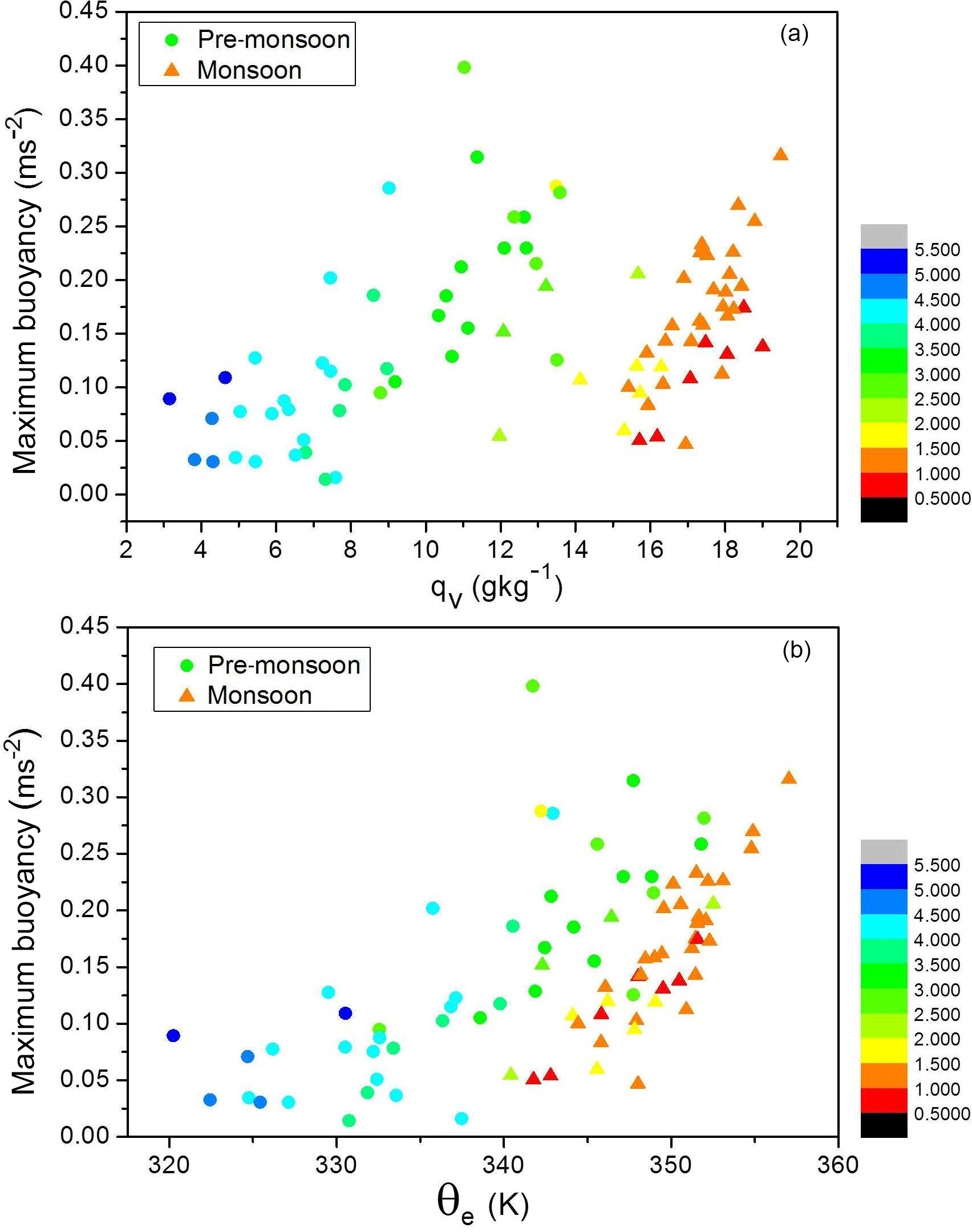
Figure 6 Variation of the maximum quasi-adiabatic buoyancy as a function of (a) surface water mixing ratio and (b) surface equivalent potential temperature. Triangular/circular symbols are for monsoon/pre-monsoon soundings, with the colour depicting the cloud base height. Pre-monsoon cases are grouped as in Figs. 4 and 5.

Figure 6 shows the maximum pseudo-adiabatic parcel buoyancy as a function of surface water vapour mixing ratio, q_v (panel a), and the surface equivalent potential temperature, θ_e (panel b). Circles (triangles) mark pre-monsoon (monsoon) conditions and the symbol colour depicts cloud base height according to the colour scale shown to the right of the panels. Overall, neither surface q_v nor surface θ_e is a good predictor of the parcel maximum buoyancy. The maximum buoyancy does seem to increase with the surface q_v, but the relationship is rather weak and there is a large scatter. The scatter reduced while soundings with similar cloud base heights are considered.

The most apparent pattern, already discussed in Sect. 3.2, is that the surface q_v strongly affects the cloud base height. The main contrast between pre-monsoon and monsoon conditions comes from a contrasting relationship in low-level temperature and humidity, that is, higher temperature and lower humidity for pre-monsoon cases, and lower temperature and higher humidity for monsoon cases. Because of compensating effects of the temperature and humidity on θ_e, its surface values are thus not a good predictor of the maximum pseudo-adiabatic parcel buoyancy either.

In summary, the availability of surface moisture seems to be a significant determinant of deep convection development over the Indian subcontinent (assuming that conditions near Pune can be taken as being representative of the rain shadow region), with pre-monsoon and monsoon conditions providing contrasting examples of the impact. Day-to-day variability of surface moisture is larger during the pre-monsoon season and it adds to the variability associated with free-tropospheric conditions, such as temperature and moisture stratification.

4 Observations of surface forcing during the pre-monsoon to monsoon transition

Since surface flux observations are not available simultaneously with Pune sounding data, we use observations collected during the IGOC campaign to contrast the role of surface forcing between pre-monsoon and monsoon conditions. As explained in Sect. 2.1, IGOC tower measurements of surface sensible and latent heat fluxes are combined with the estimates of the LCL using MWRP-derived lower tropospheric temperature and moisture profiles. Figure 7 shows evolutions of surface fluxes, the Bowen ratio, and the LCL height between 24 June and the end of July using 3-hourly data during the diurnal cycle. The pre-monsoon to monsoon transition (monsoon onset hereafter) around 1 July is clearly evident in the figure. Before the monsoon onset, the sensible heat flux is typically much larger than the latent flux, and the Bowen ratio is larger than 1. After the monsoon onset, latent and sensible fluxes reverse, with the latent heat flux becoming much larger than the sensible flux and the Bowen ratio becomes smaller than 1. The LCL height seems to decrease as Bowen ratio decreases after the monsoon onset and diurnal variations of LCL height become less significant after the monsoon onset. There seems to be a weak decreasing trend in the evolutions of the Bowen ratio and the LCL height after the monsoon onset, arguably consistent with the gradual increase of soil moisture during monsoon.

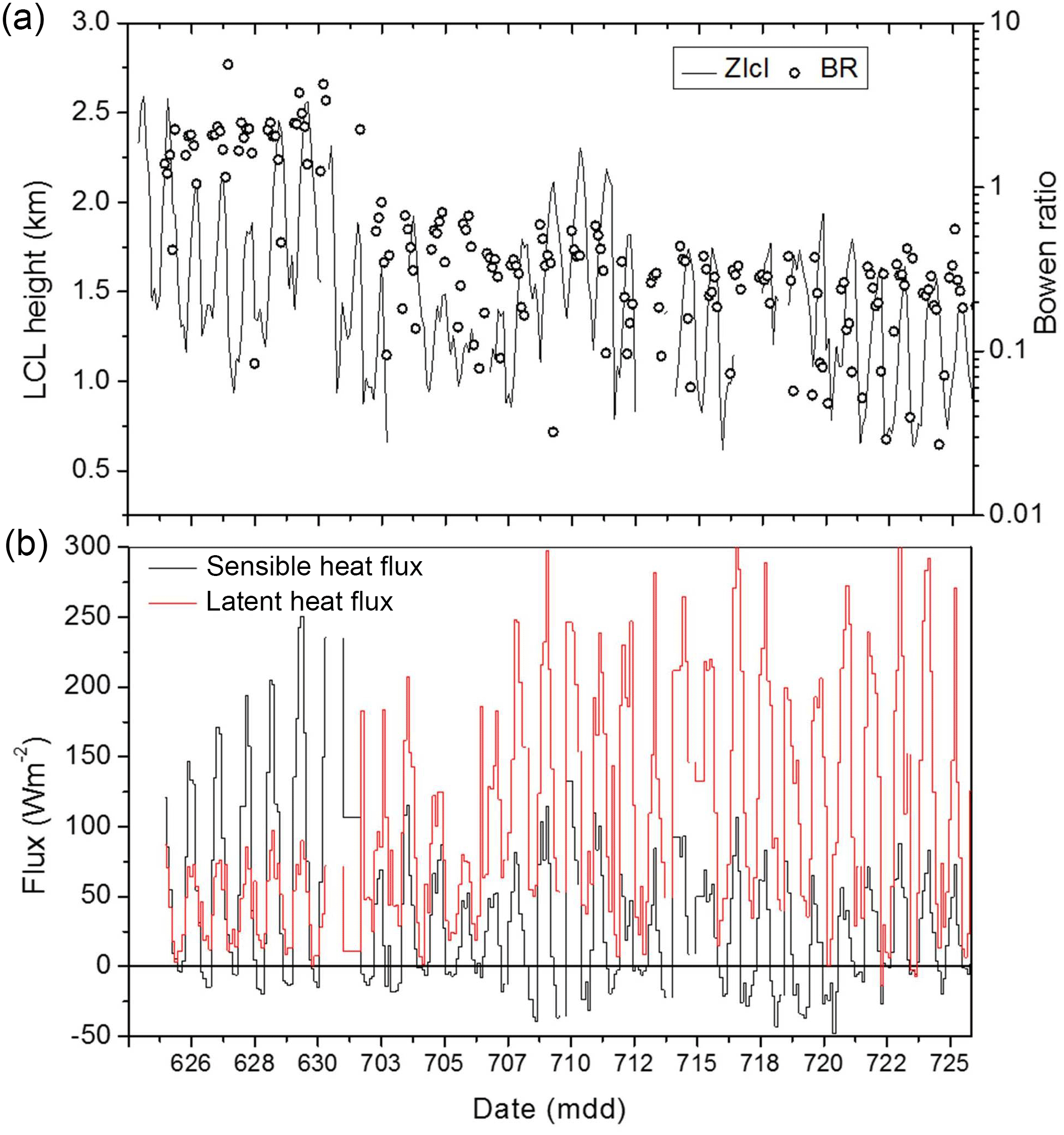
Figure 7 Evolutions of (a) the Bowen ratio (BR) and LCL height (Z_LCL) and (b) sensible (black lines) and latent (red lines) surface heat fluxes around the monsoon onset from the IGOC data.

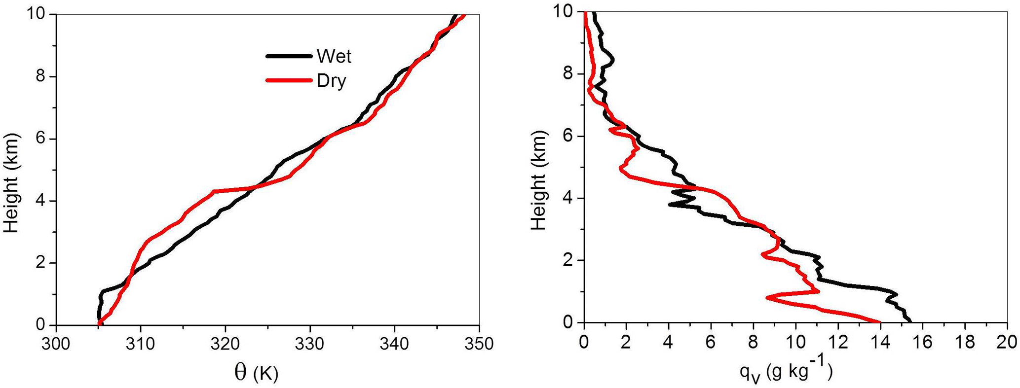
Figure 8 Vertical profile of the potential temperature and the water vapour mixing ratio used as initial conditions in the simulations for wet and dry cases from the IGOC field project.

Although IGOC flux data shown here are for a single monsoon onset case, in contrast to 5 years of sounding data, the transition from the high-Bowen ratio pre-monsoon environment to the low-Bowen ratio monsoon environment is fairly typical over the Indian subcontinent. The impact of the surface Bowen ratio on the evolution of monsoon deep convection is further illustrated by numerical simulations discussed in the next section.

5 Simulations of deep convection driven by surface forcing

Two sets of idealized simulations of moist convection with emphasis on the surface forcing are discussed in this section in support of analysis presented previously. The first pair of simulations considers monsoon convection applying two specific midday soundings from the IGOC field project, one corresponding to relatively moist surface conditions and the second corresponding to dry conditions. The soundings are from the period toward the end of monsoon, 18 September (wet case) and 2 October (dry case). As already explained, the soundings come from a radiosonde released about 1.2 km away from the surface flux tower site. The simulations are idealized because they apply midday sounding as initial conditions and use midday observed surface conditions to calculate surface fluxes, driving the simulations that are several hours long. In reality, surface conditions change because of the diurnal variations of surface insolation.

Because of such a limitation, we employ a second set of simulations that considers a daytime convective development from an early morning sounding driven by evolving surface fluxes. The simulations are based on observations in the South American Amazon region (Grabowski et al., 2006). As an illustration, we introduce a simple modification of the surface Bowen ratio and analyse its impact. Although idealized (i.e. prescribed horizontally uniform surface fluxes), the simulations provide additional illustration of the role of surface forcing in deep convection development.

5.1 Two IGOC cases of monsoon convection over India

Two contrasting soundings, referred to as wet and dry, were collected as the south-west monsoon was receding from the Indian subcontinent and the lower atmosphere was getting progressively dry. The wet case is 18 September and the dry case is 2 October. Soundings on both days were conducted around noon local time. The surface potential temperature and water vapour mixing ratio for the wet case were 305.2 K and 16.6 g kg⁻¹. Corresponding values for the dry case were 306.1 K and 13.5 g kg⁻¹. The contrasting surface temperature and moisture has been the determining factor for selecting these two cases.

Figure 8 compares the two soundings. The wet sounding features a mixed layer that is about 1 km deep (although with a noticeable vertical moisture gradient) and relatively uniform free-tropospheric stability aloft. In contrast, the dry sounding features no mixed layer near the surface and a fairly complex structure in the lowest 5 km, with distinct layers of approximately constant stability: a weakly stratified layer between the surface and about 3 km, a typically stratified layer between 3 and approximately 4.5 km, and an inversion between 4.5 and 5 km. The wet case has higher wind speed (greater than 4 m s⁻¹; not shown) compared to the dry case (smaller than 3 m s⁻¹). The mid-tropospheric inversion provides a barrier for deep convection, as illustrated by model results. The LCL height for the wet case is around 1.1 km, significantly lower than that for the dry case (around 1.6 km) due to moisture availability near the surface.

The model used for the two case simulations is the NCAR Weather Research and Forecasting (WRF) model (Skamarock et al., 2005), run in the large eddy simulation (LES) mode. The horizontal domain of 20 by 20 km² applies the 100 m grid length. The 10 km deep vertical domain is covered with a uniform grid with a 50 m vertical spacing. The model is run in an idealized manner for 8 h, applying surface fluxes derived from initial prescribed constant surface temperature and moisture values. Both simulations are initialized with radiosonde observations shown in Fig. 8. Surface conditions are prescribed from micrometeorological-tower-based observations of temperature and water vapour. The time step used in the simulation is 1 s. Since the simulations start with horizontally uniform conditions and require spin-up time to develop small-scale circulations and clouds, we present model results starting from hour 3. Figure 9 shows the evolution of surface sensible and latent heat fluxes and the Bowen ratio between hours 3 and 8. The sensible heat fluxes change little during the simulations, but latent fluxes decrease significantly, especially in the dry case. The initial total surface heat flux is about 20 W m⁻² larger in the wet case, and the difference increases as simulations progress. This implies that the surface total heat flux is larger in the wet case and the difference between two simulations increases with time. The Bowen ratio is approximately 2 at the onset of the two simulations. It remains close to 2 for the wet simulation, but increases to a value of around 12 at hour 8 for the dry case.

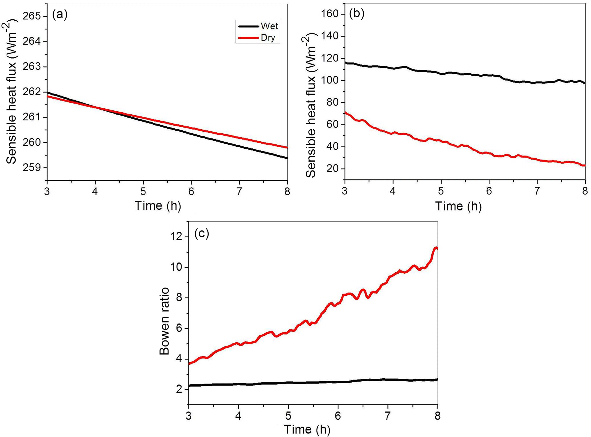
Figure 9 Evolution of (a) the sensible heat flux, (b) the latent heat flux, and (c) the Bowen ratio in simulations of dry and wet cases from the IGOC field project. Red/black lines are for the dry/wet case.

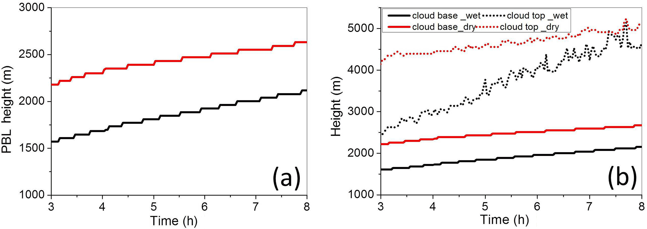
Figure 10 Evolution of (a) the planetary boundary layer (PBL) height and (b) the cloud base and cloud top heights from dry and wet simulations of the IGOC field project. Red/black lines are for the dry/wet case.

For the wet case, the initial sounding features a mixed layer that is already well identifiable (at least for the potential temperature), and the surface energy and the Bowen ratio change little throughout the simulation. Thus, the BL height increases steadily throughout the simulation, as shown in Fig. 10. The increase of boundary layer height in the wet case is accompanied by the increase of the cloud base height. The depth of the cloud field, however, increases at a higher rate, from about 2.5 km at hour 3 to about 5 km at hour 8. For the dry case, the mixed layer is absent in the initial sounding, and thus it rapidly develops during the initial couple of hours of the simulation. The BL depth is about 1 km at hour 1 (not shown) and about 2.2 km at hour 3. The rate then decreases significantly and the BL deepens subsequently at a rate comparable to the wet case, about 100 m per hour. The cloud base height rises at a similar rate, and cloud field depth remains quite steady at around 2 km between hours 3 and 8. The presence of a deep inversion between 4.5 and 5 km (see Fig. 9) provides an efficient lid for the convective development.

The changes in cloud field between hour 5 and 8 are illustrated in Fig. 11, which shows corresponding cloud fraction profiles for the two simulations. The figure illustrates the increase of cloud base heights with time, which are similar for dry and moist cases, a significant deepening of the cloud field in the moist case, and the impact of inversion between 4.5 and 5 km for the dry case, which results in almost 100 % cloud cover within the inversion.

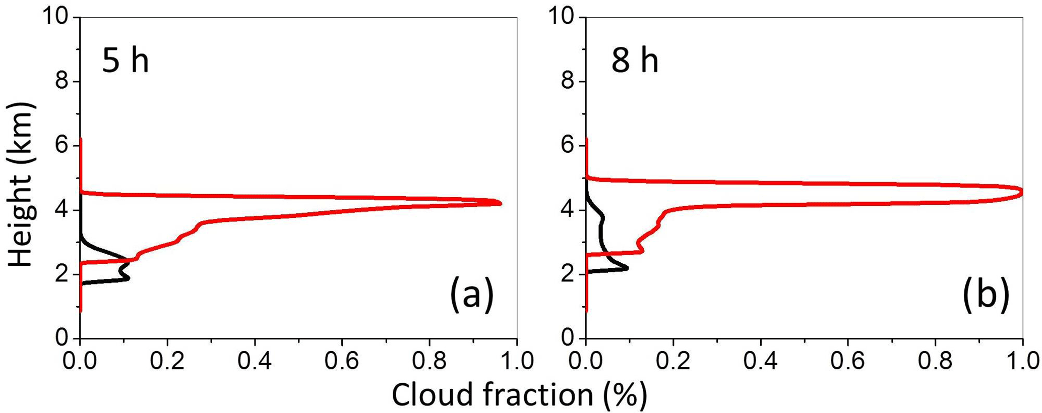
Figure 11 Cloud fraction profiles at (a) hour 5 and (b) hour 8 from dry and wet simulations of the IGOC field project. Red/black lines are for the dry/wet case.

In summary, high-resolution simulations of contrasting realistic cases observed over the Indian subcontinent illustrate the impact of surface forcing and highlight the role of specific free-tropospheric conditions in convective development and the cloud fraction. The latter are no doubt responsible, to some extent, for the observed convective environments apparent in Pune sounding data analysed in Sect. 3.

5.2 Idealized simulations of daytime convective development over land: the LBA case

Since the first set of simulations applied highly idealized forcing, we use another pair of simulations that aim at simulating daytime convective development over land, starting from the cloud-free morning sounding and finishing with the midday deep convection. We apply the case developed in Grabowski et al. (2006), whereby observations from the Amazon region motivated the design of a simple modelling case. The case features formation and deepening of the cloud-free convective boundary layer in the early morning hours, development of shallow convection in the late morning, and transition to deep convection around local noon. The 6 h simulation covers the period from 07.30 local time (approximately at sunrise) to the midday hours (13.30 local time). It starts from the horizontally homogeneous morning sounding and is forced by increasing surface latent and sensible heat fluxes mimicking effects of the increasing daytime surface insolation. This case has been used in several past studies, such as Khairoutdinov and Randall (2006), Grabowski (2015), and Grabowski and Morrison (2016, 2017). We apply the microphysical set-up based on Grabowski (1999), that is, the one referred to as IAB in Grabowski (2015).

Two simulations are performed. The first simulation, referred to as LBA (Large-Scale Biosphere–Atmosphere), follows the original set-up and features a significantly larger surface latent flux compared to the sensible flux, with the Bowen ratio between 0.4 and 0.5 as the surface fluxes evolve (this is similar to wet cases during the Indian monsoon season). Surface fluxes are switched in the second simulation; that is, the sensible flux takes values of the latent flux and the latent flux assumes values of the sensible flux. This simulation is referred to as reversed LBA, or R-LBA, and it features a surface Bowen ratio of between 2.0 and 2.5. According to Fig. 2, such a change approximately doubles the buoyancy to energy flux ratio, from about 0.4 to about 0.7. One should thus expect a significantly deeper boundary layer to develop during the course of the R-LBA simulation.

The model used in the two simulations is the same as in Grabowski (2015) and Grabowski and Morrison (2016, 2017), referred to as babyEULAG, a simplified version of the EULAG model (see http://www2.mmm.ucar.edu/eulag/, last access: 1 August 2017). Since the interest is in the boundary layer development, we apply a higher horizontal resolution with a horizontal grid length of 200 m and the same stretched vertical grid as in Grabowski (2015) and Grabowski and Morrison (2016, 2017). The horizontal domain is 24×24 km². Overall, one can argue that differences between LBA and R-LBA towards the end of the simulation should be relevant to the differences in the midday soundings between dry pre-monsoon and humid monsoon situations discussed earlier.

Figures 12 and 13 summarize results of the two simulations pertinent to the impact of the surface flux Bowen ratio on convective development. Figure 12 shows profiles of the cloud fraction in 1 h intervals from 6 h long LBA and R-LBA. Overall, the profiles evolve in a quite similar way, with only shallow clouds at hours 2 and 3, and deep convection present at hours 5 and 6. The profiles at hour 4 correspond to the shallow–deep transition period. The differences in the cloud base height in the simulations are apparent, with R-LBA (higher Bowen ratio) featuring a higher mean cloud base. Figure 13 shows the evolution of the mean cloud base height together with the evolution of the estimated height of the boundary layer. As the figure shows, the boundary layer depth is up to twice as deep in the R-LBA case than in the LBA case, especially between hours 2 and 3 and during hour 5 of these simulations. The cloud base height and the height of the boundary layer top track each other well up to the onset of significant precipitation after hour 3. The difference between the two heights is especially evident in the LBA case as the boundary layer height changes little during the two final hours. Specific differences between LBA and R-LBA in the last 2 h of the simulations may not be statistically significant due to the small domain size.

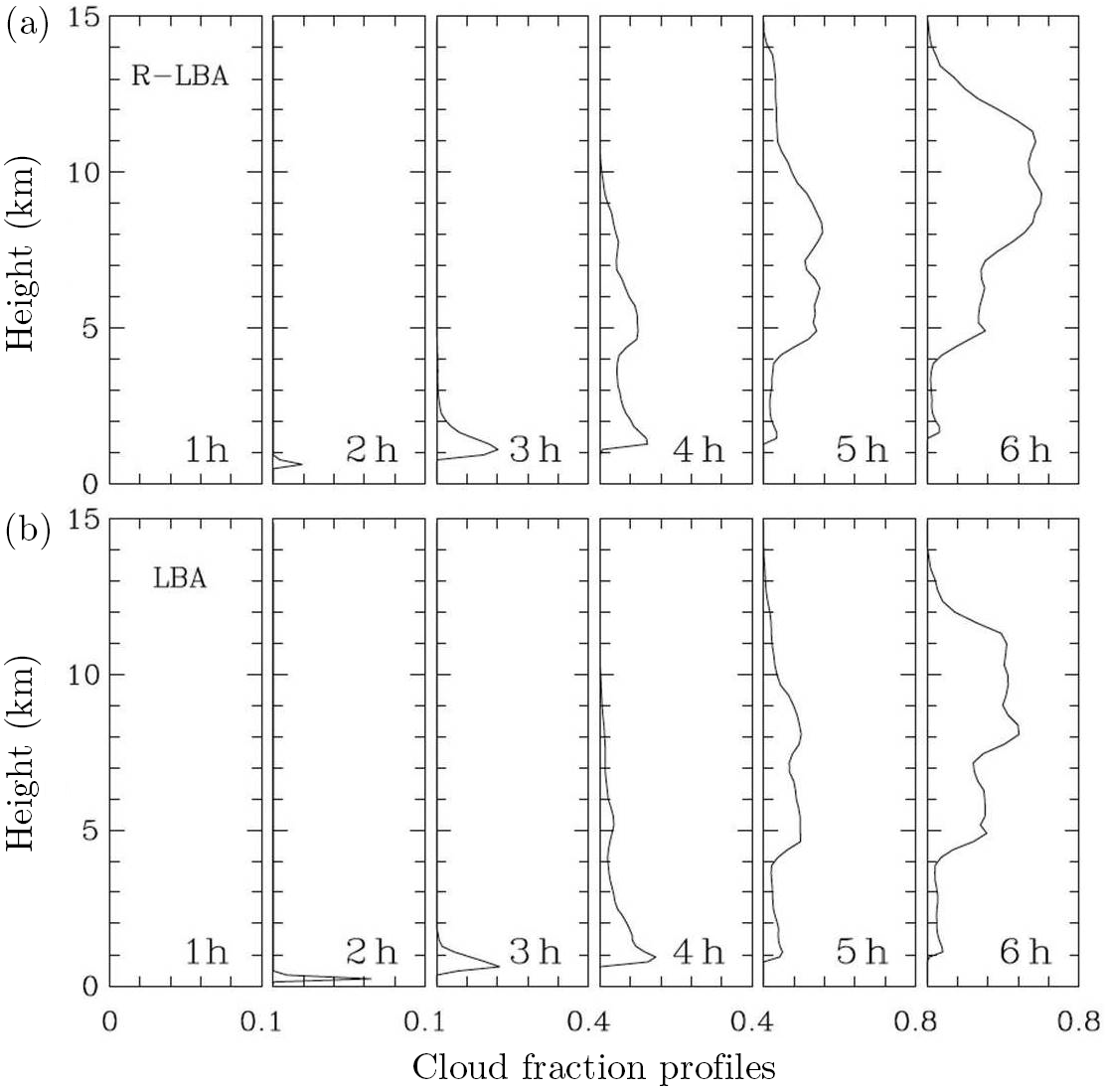
Figure 12 Cloud fraction profiles at hour 1, 2, 3, 4, 5, and 6 from (a) R-LBA and (b) LBA simulations.

Overall, differences simulated in LBA and R-LBA cases highlight the impact of the surface flux Bowen ratio and provide additional support for its role in the difference between pre-monsoon and monsoon soundings.

6 Summary

Thermodynamic soundings released around local noon for several pre-monsoon and monsoon seasons over the Indian subcontinent were analysed. Various parameters, such as the pseudo-adiabatic parcel buoyancy, the lifting condensation level (LCL), the level of free convection (LFC), the level of neutral buoyancy (LNB), convective available potential energy (CAPE), and cumulative CAPE (cCAPE), were derived by applying a pseudo-adiabatic parcel model. Overall, pre-monsoon soundings show more variability of surface and free-tropospheric conditions, as documented in Fig. 1. For the surface, the key is availability of surface moisture in both pre-monsoon and monsoon environments, whereas variability of free tropospheric temperature and humidity for the pre-monsoon is arguably because of the impact of factors other than deep convection itself, for instance, the large-scale dynamics.

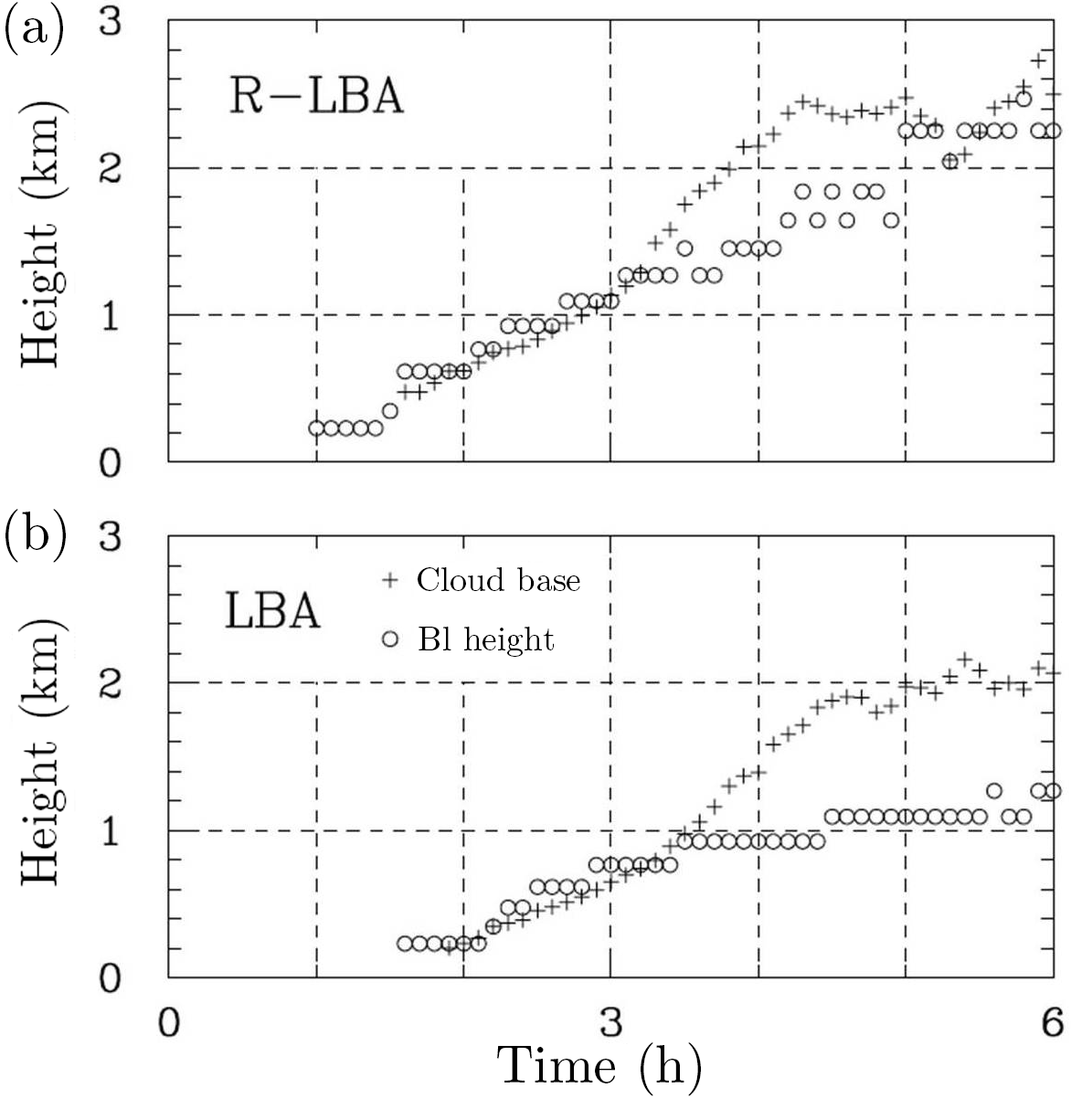
Figure 13 Evolution of the cloud base height (plus signs) and the boundary layer height (circles) in R-LBA (a) and LBA (b) simulations. Dashed lines are included to highlight differences between the simulations.

The pre-monsoon soundings feature higher cloud bases than monsoon soundings. We argue that this is a consequence of the partitioning of the surface energy flux into its sensible and latent components, as expressed by the Bowen ratio. For large Bowen ratios (the sensible surface flux is much larger than the latent flux), the ratio between the buoyancy to energy flux is close to 1; that is, all of the surface flux contributes to the buoyancy flux, which drives boundary layer dynamics. For small Bowen ratios (i.e. the sensible surface flux is much smaller than the latent flux), only about 10 % of the energy flux is used for the surface buoyancy flux (see Fig. 2). We argue that the partitioning of surface energy flux into its sensible and latent components determines variations in the LCL height as illustrated by observed rapid changes in the Bowen ratio and LCL height near the monsoon onset and illustrated in idealized numerical simulations. Observations of LCL height and the Bowen ratio during the pre-monsoon to monsoon transition illustrate rapid and concurrent changes, with the Bowen ratio and LCL height decreasing significantly as the monsoon sets in. The impact of surface forcing on the evolution of boundary layer and moist convection is also illustrated through numerical simulations that complement sounding analysis.

The sounding data show that LCL height is linearly related to surface-level moisture content with some scatter around the perfect linear relationship (Fig. 3a). The scatter is eliminated when surface-level relative humidity (RH) is used as a measure of surface layer moisture content (Fig. 3b). A theoretical basis for such a relationship is developed; see Eq. (3). The theoretical relationship between LCL height and surface-level RH mimics the relationship obtained with the parcel model. However, a significant offset is present between the theoretical LCL height and the LCL predicted by the parcel model. The offset is argued to most likely come from the presence of the surface superadiabatic layer not considered in the theoretical argument. The general consistency between theoretical and parcel-model-derived relationships between LCL height and surface moisture (Fig. 3) supports the conjecture that surface forcing determines LCL height. This should be expected in high-insolation pre-monsoon and monsoon conditions, when surface forcing due to the diurnal cycle drives the formation of a well-mixed convective boundary layer in the morning and development of deep convection at later hours.

Overall, the LNB and CAPE vary more for the pre-monsoon soundings. Large CAPE pre-monsoon soundings are characterized by maximum pseudo-adiabatic parcel buoyancies that are similar to monsoon soundings. With a few monsoon exceptions, a low LNB and thus low CAPE soundings are present only for the pre-monsoon environment. For both pre-monsoon and monsoon soundings, the LNB and CAPE are linearly related to the surface q_v with a larger scatter for the pre-monsoon environment. In general, neither surface q_v nor surface θ_e are good predictors of the parcel maximum pseudo-adiabatic buoyancy, although there is a general increase of the maximum buoyancy and CAPE with the increase of either the surface q_v or θ_e. The increase is along different paths for pre-monsoon and monsoon soundings; see Figs. 4 and 5. The scatter is small for monsoon cases, no doubt because of smaller variability of free-tropospheric structure as documented in Fig. 1.

In this study, we consider changes of the Bowen ratio as the controlling factor rather than the effect of monsoon precipitation. Because monsoon precipitation changes the surface moisture availability, the Bowen ratio is both the effect (say, on longer timescales) and the cause (say, on a daily timescale) of the differences in convection and precipitation. This brings the issue of the soil–precipitation (S–P) feedback. Land surface parameters, such as soil moisture and vegetation cover, collectively determine the surface energy balance that influences turbulent motion and the boundary layer depth (Jones and Brunsell, 2009). Arguably, of all the surface properties, soil moisture has the largest impact on the Bowen ratio. Soil moisture has the memory of atmospheric processes (Orlowsky and Seneviratne, 2010), it responds to precipitation variability, and it affects precipitation through evaporation (Douville et al., 2001). The S–P feedback has been studied in the past for the Indian monsoon region. For instance, Asharaf et al. (2012) found that the pre-monsoon soil moisture significantly influences monsoonal precipitation. However, for a single day, the Bowen ratio acts as the controlling factor, especially for the semi-arid region presented in the present study. This has been demonstrated in several studies. Rabin et al. (1990) studied the observed variability of clouds over a landscape using a one-dimensional parcel model, attributing changes in cloudiness to changes in the Bowen ratio. Our study points to previous findings by Rabin (1977), which note that on moist days clouds develop earlier over places with a low Bowen ratio, and on dry days convection occurs sooner over regions with a higher Bowen ratio. Lewellen et al. (1996) considered the impact of the Bowen ratio on boundary layer clouds using LESs. They suggest that lower cloud ceilings occur for low values of the Bowen ratio. Schär et al. (1999) conducted simulations using a regional climate model focusing on the S–P feedback and noticed that wet soils with a small Bowen ratio produces shallow boundary layer. All these studies are consistent with the picture emerging from our analysis.

It may be important to mention that soil moisture has different scales of variability from a few minutes to several months and carries the memory into subsequent seasons. The surface fluxes are also controlled by the net insolation. Although the latent heat flux remains high during the monsoon period, the sensible heat flux increases during the break periods and this leads to slight variations in the Bowen ratio, as indicated in Fig. 7. However, during the monsoon season, the Bowen ratio stays close to 2, mostly due to a consistently high latent heat flux. It comes from both the surface and vegetation through evapotranspiration. Consistent cloudiness during the season reduces incident radiation, which gives a lower sensible heat flux. A detailed study of surface fluxes and relation with clouds and radiation can be found in Urankar et al. (2012), indicating that clouds also have a significant feedback on the surface energy budget.

This study is not adequate to explain active and break period characteristics of monsoon convective environments. Relevant studies concerning monsoon active and break periods (e.g. Pai et al., 2016; Rajeevan et al., 2010) introduce classification based on the weather properties over the monsoon core region that covers most of central India. Our study considers high-resolution radiosonde measurements, for which the data are collected over a single location over the Indian subcontinent. The local data are insufficient to explain active break conditions because of the significant spatio-temporal variability of the monsoon.

Finally, results presented in this paper should help to understand effects of aerosols, dramatically different between the highly polluted pre-monsoon environment and the relatively clean environment during the monsoon, on moist convection over the Indian subcontinent. Understanding dynamical effects, for instance, partitioning of the surface heat flux into its sensible and latent components and how the partitioning affects the cloud base height and cloud buoyancy, is required for a confident selection of deep convection cases suitable for cloud seeding, the target of the ongoing Indian precipitation enhancement programme (Prabha et al., 2011; Kulkarni et al., 2012; Prabha, 2014).