the Creative Commons Attribution 4.0 License.
the Creative Commons Attribution 4.0 License.
 | 14 May 2018
Quantifying the effect of mixing on the mean age of air in CCMVal-2 and CCMI-1 models
Simone Dietmüller
Roland Eichinger
Hella Garny
Thomas Birner
Harald Boenisch
Giovanni Pitari
Eva Mancini
Daniele Visioni
Andrea Stenke
Laura Revell
Eugene Rozanov
David A. Plummer
John Scinocca
Patrick Jöckel
Luke Oman
Makoto Deushi
Shibata Kiyotaka
Douglas E. Kinnison
Rolando Garcia
Olaf Morgenstern
Guang Zeng
Kane Adam Stone
Robyn Schofield
The stratospheric age of air (AoA) is a useful measure of the overall capabilities of a general circulation model (GCM) to simulate stratospheric transport. Previous studies have reported a large spread in the simulation of AoA by GCMs and coupled chemistry–climate models (CCMs). Compared to observational estimates, simulated AoA is mostly too low. Here we attempt to untangle the processes that lead to the AoA differences between the models and between models and observations. AoA is influenced by both mean transport by the residual circulation and two-way mixing; we quantify the effects of these processes using data from the CCM inter-comparison projects CCMVal-2 (Chemistry–Climate Model Validation Activity 2) and CCMI-1 (Chemistry–Climate Model Initiative, phase 1). Transport along the residual circulation is measured by the residual circulation transit time (RCTT). We interpret the difference between AoA and RCTT as additional aging by mixing. Aging by mixing thus includes mixing on both the resolved and subgrid scale. We find that the spread in AoA between the models is primarily caused by differences in the effects of mixing and only to some extent by differences in residual circulation strength. These effects are quantified by the mixing efficiency, a measure of the relative increase in AoA by mixing. The mixing efficiency varies strongly between the models from 0.24 to 1.02. We show that the mixing efficiency is not only controlled by horizontal mixing, but by vertical mixing and vertical diffusion as well. Possible causes for the differences in the models' mixing efficiencies are discussed. Differences in subgrid-scale mixing (including differences in advection schemes and model resolutions) likely contribute to the differences in mixing efficiency. However, differences in the relative contribution of resolved versus parameterized wave forcing do not appear to be related to differences in mixing efficiency or AoA.
- Article
(3484 KB) - Full-text XML
-
Supplement
(210 KB) - BibTeX
- EndNote


The Brewer–Dobson circulation (BDC) affects the stratospheric distribution of radiative active trace gases, which strongly contribute to the radiative forcing of the climate system. Stratospheric mean age of air (AoA) is defined as the mean transport time of an air parcel from the entry region at the tropical tropopause to any region in the stratosphere (Hall and Plumb, 1994; Waugh and Hall, 2002). AoA is a useful measure for the analysis of stratospheric transport, as it includes both the effects of the slow overturning residual circulation and the effect of the two-way mass exchange of air parcels, referred to as (eddy) mixing (e.g., Butchart, 2014). AoA can also be derived from observations of conserved tracers whose tropospheric concentrations increase approximately linearly over time, such as balloon-borne and satellite observations of SF6 or CO2 mixing ratios (e.g., Andrews et al., 2001; Engel et al., 2009, 2017; Stiller et al., 2012; Haenel et al., 2015). AoA derived from observations then can be directly compared to AoA simulated by general circulation models (GCMs) and chemistry–climate models (CCMs) (as done, for example, in Eyring et al., 2006; SPARC, 2010). The concept of stratospheric AoA is very helpful, as it is a possible observation-based measure of the BDC. However, it is important to note that the AoA diagnostic bears information on both mean residual circulation and effects of two-way mixing, as it is the integrated effect of all transport processes.
In the past model inter-comparison studies with GCMs, chemical transport models (CTMs) and CCMs (e.g., Hall et al., 1999; Eyring et al., 2006; Butchart et al., 2010) showed a significant model spread in AoA. In comparison to observations, simulated AoA was too low in many models, mainly in the middle and upper stratosphere. The model inter-comparison activity CCMVal-2 (Chemistry–Climate Model Validation Activity 2) was conducted with the goal of improving the understanding of stratosphere-resolving CCMs. In the SPARC (Stratospheric Processes and their Role in Climate Project) CCMVal-2 report (SPARC, 2010) the AoA diagnostics of 15 CCMVal-2 models were analyzed at a wide range of latitudes and altitudes. The models' AoA was compared to in situ observations of Andrews et al. (2001) and Engel et al. (2009) (see the tropical and midlatitude AoA profiles and the latitudinal AoA distribution at 50 hPa in Fig. 5.5 of SPARC, 2010). It was shown that 7 out of 15 models match closely the observed AoA at 50 hPa at all latitudes and also their vertical tropical AoA profiles are within the uncertainties of the observations at all altitudes. However, for most of these models AoA is too low in the middle stratosphere when compared to in situ observations. Moreover, the spread of simulated AoA between the models is high.
To understand the model spread in AoA and their discrepancy to observations, the processes that drive stratospheric transport need to be disentangled, namely the effects of residual transport and mixing. Several methods for this separation have been used. Ray et al. (2010) have used a methodology based on the conceptual one-dimensional tropical leaky pipe (TLP) model (see Neu and Plumb, 1999) to constrain the circulation strength and mixing strength across the subtropical barrier in a model by observed concentrations of long-lived tracers. In SPARC (2010) several diagnostics were employed to measure transport characteristics like tropical ascent or tropical to midlatitude mixing. Those diagnostics were based on tracer concentrations, allowing for a comparison to observations. However, with most diagnostics it is not possible to entirely separate the different effects. It was found that most models appear to have too-strong tropical-to-midlatitude mixing and too-fast tropical ascent. As those two biases compensate, it is argued that despite those model biases a reasonable AoA can be produced in the models. Overall, a good relationship between the model's ability to simulate mean AoA to the ability to simulate both tropical lower stratospheric ascent and tropical-midlatitude mixing was found (see SPARC, 2010, their Fig. 5.20).
Previous studies have developed diagnostics to measure dispersive stratospheric transport associated with eddy mixing (e.g., Newman et al., 1986; Nakamura, 1996; Haynes and Shuckburgh, 2000). Transport times, i. e. AoA, are affected by the path-integrated effects of local eddy mixing. Several theoretical concept studies with idealized models found that overall mixing increases AoA due to enhanced re-circulation (e.g., Hall and Plumb, 1994; Neu and Plumb, 1999). More recent studies have developed diagnostics to quantify the effect of mixing on AoA from global model data (e.g., Garny et al., 2014; Ploeger et al., 2015b; Dietmüller et al., 2017). Garny et al. (2014) quantified the effect of mixing on AoA (termed as aging by mixing) with the global climate model ECHAM6 (European Centre/Hamburg version 6). They analyzed the difference of simulated AoA and the transit time of the hypothetical transport along the residual circulation only (in the following termed as residual circulation transit time, RCTT). They found that additional aging by mixing can be found in most of the stratosphere, because mixing between the tropics and extratropics causes air to recirculate, and thus AoA is increased. Only in the lowermost stratosphere, where air mass exchange with young tropospheric air occurs, mixing leads to a reduction of AoA. Ploeger et al. (2015b) confirmed these results with the Lagrangian chemistry transport model CLaMS (Chemical Lagrangian Model of the Stratosphere) by explicitly calculating aging by mixing on resolved scales through integration of local eddy mixing tendencies along the residual circulation trajectories. In the explicit calculation of aging by mixing, parameterized and numerical diffusion are not included. Dietmüller et al. (2017) combined the two methods of calculating aging by mixing and thus the effects of resolved and unresolved mixing on AoA (latter termed aging by diffusion) can be separated. By analyzing simulation data of the CCM EMAC (ECHAM/MESSy Atmospheric Chemistry) and of CLaMS, they found that aging by diffusion enhances AoA, contradicting some previous thoughts, which assumed that diffusion makes air younger (e.g., Eluszkiewicz et al., 2000; Waugh and Hall, 2002; SPARC, 2010). However, the contribution of unresolved mixing was found to only play a minor role (impact of 5–10 % on AoA) in both models.
By applying the concept of the idealized TLP model, Garny et al. (2014) derived the so-called “mixing efficiency”. The mixing efficiency is defined as the ratio of the two-way mixing mass flux across the subtropical barrier to the net residual mass flux. This mixing efficiency controls the ratio of tropical mean AoA to RCTT and thus describes the relative increase in AoA by mixing. Garny et al. (2014) investigated the mixing efficiency for three different climate equilibrium states (pre-industrial – 1860, present-day – 1990, and future – 2050) and found that the strength of two-way mixing is tightly coupled to the strength of the lower stratospheric residual circulation. The ratio of mixing strength to residual circulation strength is almost constant in the three different climate states (i.e., the mixing efficiency is constant). Garny et al. (2014) proposed that the comparison of the relative aging by mixing (or of the mixing efficiency) between models can provide useful insights in the widely known model deficits in the AoA simulation.
Scinocca et al. (2008)Pawson et al. (2008)Jourdain et al. (2008)Shibata and Deushi (2008)Schraner et al. (2008)Pitari et al. (2002)Morgenstern et al. (2009)Garcia et al. (2007)Morgenstern et al. (2009, 2013)Stone et al. (2016)Jonsson et al. (2004)Scinocca et al. (2008)Solomon et al. (2015)Garcia et al. (2017)Marsh et al. (2013)Jöckel et al. (2010, 2016)Jöckel et al. (2010, 2016)Molod et al. (2012, 2015)Oman et al. (2011, 2013)Deushi and Shibata (2011)Yukimoto et al. (2011, 2012)Stenke et al. (2013)Revell et al. (2015)Morgenstern et al. (2009, 2013)Stone et al. (2016)Pitari et al. (2014)Table 1Overview of the CCMs and their simulation setups used in the present study. The reference(s), the horizontal and vertical resolution (number of model layers), and the model top and the advection schemes (of chemical tracers) of the individual models of CCMVal-2 (upper rows) and CCMI-1 (lower rows) are listed. For the spectral models, horizontal resolution is given as triangular truncation of the spectral domain, with T21 ≈ 5.65∘ × 5.65∘, T30/T32 ≈ 3.75∘ × 3.75∘, T42 ≈ 2.8∘ × 2.8∘ and T47 ≈ 2.5∘ × 2.5∘. TL159 ≈ 1.1∘ × 1.1∘ The advection schemes are as follows SP is spectral, FFSL is flux-form semi-Lagrangian, SL is semi-Lagrangian, STFD is spectral transform and finite difference, FFEE is flux-form Eulerian explicit, FV is finite volume (for details see SPARC, 2010).
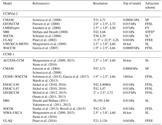
∗ These models use different transport schemes for meteorological tracers.
In this study we seek to gain a better quantitative understanding of the processes that control the BDC, in order to explain the differences in climatological AoA between CCMs. To do so the effects of residual transport and of mixing on AoA are analyzed and investigated for various recent CCMs. We use the data of the hindcast simulations of the inter-comparison projects CCMVal-2 and CCMI-1 (Chemistry–Climate Model Initiative, phase 1). A brief description of the models and simulations is presented in Sect. 2. The methods of calculating AoA, RCTT, aging by mixing, the mixing efficiency and tropical upwelling are shortly introduced in Sect. 3. Annual mean AoA, RCTT, aging by mixing and mixing efficiency are analyzed in Sect. 4. In Sect. 5 we discuss possible causes for the inter-model differences in mixing, including effects of vertical dispersion and model characteristics. A summary and concluding remarks are given in Sect. 6.
In the present study, we analyze the model output from 17 state-of-the-art CCM simulations. The output of eight simulations is obtained from the coordinated model inter-comparison Chemistry–Climate Model Validation Activity 2 (Morgenstern et al., 2010; Eyring et al., 2006) and the output of the other nine simulations from the ongoing Chemistry–Climate Model Initiative phase 1 (Eyring et al., 2013; Morgenstern et al., 2017). A list of these CCMs is provided in Table 1, together with references and relevant information on the model setups, namely the vertical and horizontal resolution, the height of the model top and the advection scheme. This subset of models that contributed to CCMVal-2 and CCMI-1 is chosen according to the availability of the necessary data (AoA and residual circulation velocities).
In the following, we briefly describe some aspects of the CCMs that are relevant for our study. A detailed overview of all models that participated in CCMVal-2 and CCMI-1 is provided by Morgenstern et al. (2010, 2017). Note that many CCMI-1 models have a predecessor model in CCMVal-2, thus the development since CCMVal-2 (e.g., improvements in chemistry and physics or higher resolution) can be studied. Note also that there are family relationships between different models; e.g., the models ACCESS-CCM and NIWA-UKCA are identical and the models EMAC and SOCOL are both based on the ECHAM5 climate model. Moreover, we use the EMAC model in two different vertical resolutions (i.e., EMAC-L47 and EMAC-L90MA).
The models' horizontal resolutions vary between ∼ 5 and ∼ 2∘ and the vertical resolutions range from 26 to 126 levels with the top of the different models from 0.07 up to 0.00005 hPa.
Several types of advection schemes are used in the CCMVal-2 and CCMI-1 models. Numerical diffusion in GCMs is linked to the discrete nature of grids which are used for transport processes. Generally, advection schemes are designed to minimize numerical diffusion; however, for stability reasons several models require explicit diffusion (Morgenstern et al., 2010, 2017). The different advection schemes are also provided in Table 1. Note that in CCMVal-2 there are two models (MRI and SOCOL) that use different schemes for meteorological and chemical tracers. Thus, in these models, the advection of the different types of tracers is physically not self-consistent (Morgenstern et al., 2010). The SOCOL model has changed the advection scheme between CCMVal-2 and CCMI-1. Differences in the advection scheme may cause differences in the distribution of chemical species and AoA, particularly in the lower stratosphere (Morgenstern et al., 2010; Eluszkiewicz et al., 2000).
The BDC is driven by the momentum deposition of breaking waves (Haynes et al., 1991) with small-scale gravity waves contributing significantly, but these small-scale waves are not resolved in most GCMs. Numerous parameterization schemes for the calculation of gravity wave drag (GWD) are applied in the different CCMVal-2 and CCMI-1 models. Based on the generation of the gravity wave scheme, the computation of their drag is separated into orographic and non-orographic parameterization schemes. For the non-orographic gravity wave drag (NOGWD), various methods are used to determine the sources as well as the launch levels of the gravity waves. The gravity wave schemes used by the different models are listed in Table S9 of Morgenstern et al. (2017) and in Table 3 of Morgenstern et al. (2010).
The simulations evaluated here are the long transient (free running) reference simulations REF-B1 of CCMVal-2 (covering the recent past from 1960 to 2006) and REF-C1 of CCMI-1 (covering the recent past from 1960 to 2010). The long-term mean over those years provides the base for our inter-comparison. The REF-B1 and REF-C1 reference simulations were performed analogously, using observational forcings, including all anthropogenic and natural forcings based on changes in trace gases, solar variability, volcanic eruptions and sea surface temperatures. Some of these forcings, however, differ between CCMVal-2 and CCMI-1. All details of the REF-B1 and REF-C1 simulations are documented by Morgenstern et al. (2010, 2017) and follow the designs of Eyring et al. (2006) or Eyring et al. (2013).
3.1 Calculation of AoA, RCTT and aging by mixing
Stratospheric mean age of air is defined as the transit time of air parcels in the stratosphere, starting at the tropical tropopause (e.g Hall and Plumb, 1994; Waugh and Hall, 2002) and is affected both by the residual circulation and by eddy mixing. In almost all CCMs, the AoA tracer is implemented as an inert tracer with prescribed lower boundary conditions (in some models the lower boundary condition is applied globally and in others only in the tropics) that linearly increase in mixing ratio over time (“clock-tracer”; Hall and Plumb, 1994). Diagnosed AoA at a certain grid point in the stratosphere is then calculated as the time lag between the local tracer mixing ratio (at this certain grid point) and the current mixing ratio at a reference point. As this reference point does vary among the models (e.g., boundary layer, tropical thermal tropopause, 100hPa), we subtract the AoA value at each model's individual tropical thermal tropopause from AoA (so that AoA = 0 there) to obtain consistency between the models. Only the CCMVal-2 model CMAM uses a stratospheric source AoA tracer (for details see SPARC, 2010).
The residual circulation transit time is the hypothetical age air would have if it were only transported by the residual circulation, i.e., without eddy mixing. RCTTs are calculated following Birner and Bönisch (2011) by calculating backward trajectories that are driven by the transformed Eulerian-mean (TEM) meridional and vertical monthly velocities ( and , referred to as residual velocities) with a standard fourth-order Runge–Kutta integration. The backward trajectories are initialized on a latitude pressure grid (depending on the model). The residual velocities are available in the CCMI-1 and CCMVal-2 data base. The backward trajectories are terminated when they reach the thermal tropopause. The elapsed time is then the residual circulation transit time. A detailed description is given by Birner and Bönisch (2011) and by Garny et al. (2014). It is important to mention here that the calculation of is treated inconsistently within the different models, as in some models a fixed-scale height was used to transform from Pa s−1 to m s−1, while in other models the actual density was used for this transformation. The different calculation methods of can lead to significant differences in (e.g., 17 % at 70 hPa for EMAC). To facilitate a quantitative model comparison we thus recalculated from the given fields using the continuity equation for all models. Further details are given in the Supplement of this paper.
Besides the transport by the residual circulation, AoA is affected by eddy mixing (Neu and Plumb, 1999; Garny et al., 2014; Ploeger et al., 2015b, a). As pointed out by Garny et al. (2014), mixing of air from the midlatitudes into the tropical pipe can cause additional aging through recirculation of aged air. This process is called aging by mixing. In their study, Garny et al. (2014) proposed that in global models aging by mixing can be interpreted as the difference between simulated AoA and RCTT. However, it has to be taken into account that aging by mixing obtained as the difference between AoA and RCTT includes mixing on unresolved scales (namely parameterized and numerical diffusion).
3.2 TLP model and mixing efficiency
We use the concept of the tropical leaky pipe model (Neu and Plumb, 1999) to better understand the contribution of different processes to AoA. The TLP model is a simple one-dimensional conceptual model of stratospheric transport, which includes advection and horizontal two-way mixing between tropics and extratropics across the subtropical barrier. When neglecting vertical diffusion, an analytical solution for tropical and midlatitude AoA can be formulated. The solution of the TLP model with height-dependent tropical vertical velocity for tropical AoA (AoAT) is defined as follows:
Here H stands for the scale height (7 km), α for the ratio of tropical to extratropical mass, zT for the height of the tropical tropopause and . From Eq. (1) it is clear that the two free parameters that AoA depends on are the advective vertical velocity (i.e., the residual velocity ) and the amount of mixing between the tropics and extratropics, controlled by the so-called mixing efficiency ϵ. The mixing efficiency is defined as the ratio of the mixing mass flux to the net mass flux across the subtropical barrier. Solving Eq. (1) for the mixing efficiency gives ; i.e., the mixing efficiency is approximately proportional to the relative increase in AoA by mixing. Thus, mixing efficiency is a useful measure of the relative mixing effects (see Garny et al., 2014). The mixing efficiency is calculated as the best fit of Eq. (1) to the tropical profiles of AoA and from the model data over a certain height range. The tropical profiles are averaged over the latitudinal band of 20∘ S–20∘ N (sensitivity to the width of the tropical band is discussed in Sect. 4) and are interpolated to vertical coordinates relative to the tropopause height of each model, and the fit is performed for the altitude range from the tropopause to 32 km (details for the calculation of the mixing efficiency are given in Garny et al., 2014).
To analyze the role of vertical diffusion for AoA profiles and the derived mixing efficiency (see Sect. 5.1) the TLP model is implemented as Lagrangian model (following Ray et al., 2014). Briefly, the model consists of three vertical “pipes” (tropics, northern hemisphere, NH, and southern hemisphere, SH), and particles are injected in the tropics, advected vertically with given vertical winds, and exchanged between tropics and the NH and SH extratropics. Horizontal advection and mixing is modeled as a Bernoulli process based on probabilities of parcel exchange. Vertical diffusion (which is neglected in the analytical TLP solution) is implemented as random walk: the height of each parcel i is calculated as , where ζ is a random displacement drawn from a Gaussian distribution with zero mean and variance σ2=2Kδt (where K is the vertical diffusivity at this height; see Ghoniem and Sherman, 1985).
3.3 Tropical upwelling
The stratospheric circulation is driven by the dissipation of waves that propagate upwards from the troposphere to the stratosphere. As measure for the strength of the residual circulation, the strength of tropical upwelling is commonly used (Holton et al., 1995). Here, we use the quasi-geostrophic approximation of the transformed Eulerian-mean equations to calculate the streamfunction of the residual circulation driven by the Eliassen–Palm flux divergence (EPFD) and the sum of orographic and non-orographic gravity wave drag (OGWD and NOGWD) as follows:
Here, F denotes the Eliassen–Palm flux, the total zonal gravity wave drag, f the coriolis parameter, ϕ the given latitude, p the given pressure and the meridional gradient of the zonal mean angular momentum. Tropical upwelling is then given by the difference in the residual streamfunction at the tropical boundaries (20∘ S, 20∘ N). This calculation linearly separates the influence of resolved planetary wave driving (EPFD: ) and unresolved gravity wave drag (GWD: ) on tropical upwelling. This can provide insights into the driving mechanisms of stratospheric transport and mixing variations, and thereby in AoA spread among the models.
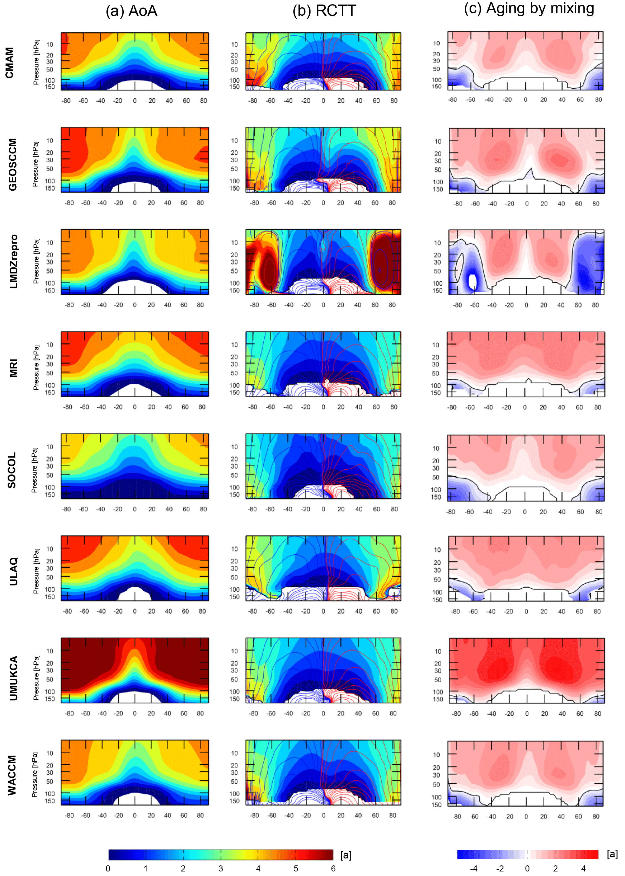
Figure 1Zonal annual mean of (a) AoA, (b) RCTT and (c) aging by mixing. Annual means show the average over the years 1980–2006 for the REF-B1 simulations of CCMVal-2. Units are given in years. Annual mean residual circulation is overlaid over the RCTT patterns (blue and red lines).
4.1 AoA, RCTT and aging by mixing
The long-term climatological mean AoA, RCTT, and aging by mixing are calculated for each model listed in Table 1 and are shown in Fig. 1 for the CCMVal-2 models and in Fig. 2 for the CCMI-1 models. Additionally, the residual circulation is overlaid in the RCTT panels. The climatological means are calculated over the years 1980 to 2006 for CCMVal-2 REF-B1 models and from 1980 to 2010 for CCMI REF-C1 models, because all available simulations overlap in this period. In general, the zonal annual mean patterns of AoA of all CCMs (Figs. 1 and 2, left panel) agree qualitatively in the typical AoA distribution. All models have lower AoA in the tropical lower stratosphere and old air in the extra-tropical middle stratosphere. However, the simulated magnitude of AoA shows large variations among the different models of CCMVal-2 and CCMI-1, mainly at high latitudes in the upper stratosphere. In this region, the AoA values range between 4.0 and 6.5 years. Generally, the highest AoA values are found in the UMUKCA-METO (CCMVal-2), lying far outside of the model spread. For the CCMVal-2 models (Fig. 1), besides the UMUKCA-METO model, the ULAQ and MRI models simulated rather high AoA values and the SOCOL model has the lowest AoA values. Within the CCMI-1 models, EMAC and MRI are on the high side of AoA values, whereas the models NIWA-UKCA, SOCOL, ULAQ and WACCM are on the low side. Furthermore, differences in the shape of the AoA isopleths between the analyzed CCMs are apparent, ranging from peaked to flat gradients. Figures 1 and 2 show strong horizontal gradients for the models GEOSCCM and UMUKCA-METO of CCMVal-2 and for the model MRI of CCMI-1 as well as low gradients for the model SOCOL of CCMVal-2 and for the models NIWA-UKCA, SOCOL and ULAQ of CCMI-1. Note that the CCMs NIWA-UMUKCA and ACCESS are identical and use the same model setup for the REF-C1 simulations; however, they were conducted on two different platforms. We found that the two model runs are climatologically identical for dynamics (as seen, for example, for upwelling, residual circulation and zonal winds) and also for transport-determined tracers (e.g., CH4). However, there are significant differences in AoA between the two models (with considerably lower AoA in ACCESS), which we can currently not explain. If the platform dependence was the reason for differences in transport, we would expect to find similar differences in other tracers. Therefore, we will only show the results of NIWA-UMUKCA in the following.

Figure 2As Fig. 1, but annual means show the average over the years 1980–2010 for the REF-C1 simulations of CCMI-1.
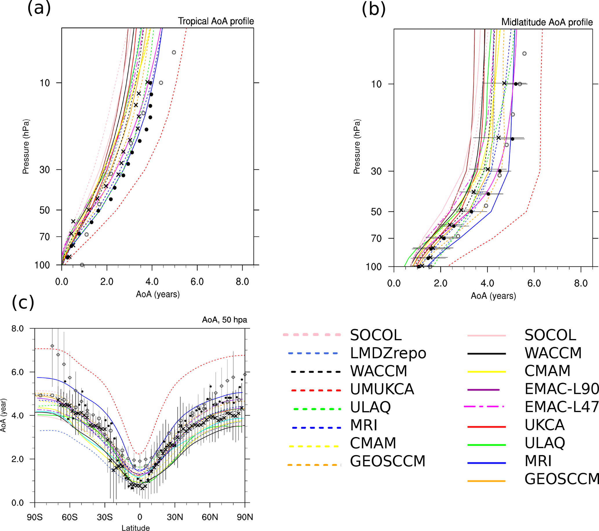
Figure 3(a) Tropical (10∘ N–10∘ S) AoA profile, (b) midlatitude (35–45∘ N) AoA profile and (c) latitudinal AoA distribution at 50 hPa for all analyzed CCMVal-2 models (dashed lines) and CCMI-1 models (solid line), with AoA averaged over the years 1980–2006. AoA profiles are shown together with the observational AoA data derived from airborne in situ measurements of SF6 (black dots) and CO2 (black crosses). For the extra-tropics the observations from Engel et al. (2009) and for the tropics the observations of Andrews et al. (2001) are used. Uncertainties of the observational data of Engel et al. (2009) are shown as 1σ. Observational data of Andrews et al. (2001) were not reported with uncertainties. Moreover, AoA determined from GOZCARDS N2O data is used (gray circles) (Andrews et al., 2001; Linz et al., 2017). The latitudinal AoA distribution is shown together with AoA from MIPAS SF6 data (gray diamond symbols), with AoA from GOZCARDS N2O data (gray circle) and with in situ measurements of Andrews et al. (2001) (black cross for CO2 and black dot for SF6). Error bars of the observational MIPAS data at 50 hPa give the range between minimum and maximum values.
For a more quantitative comparison, we show (analogously to chap. 5 of SPARC, 2010) the tropical (10∘ N–10∘ S) and midlatitude (35–45∘ N) annual mean AoA profile and the latitudinal distribution of AoA at 50 hPa for all analyzed CCMs together with the available observed AoA profiles in Fig. 3. The observational data are obtained from airborne in situ observations of the SF6 and CO2 profiles from different measurement campaigns during the last decades (Andrews et al., 2001; Engel et al., 2009, 2017). For the midlatitudes we use the AoA profiles of Engel et al. (2009) and for the tropics the AoA profiles of Andrews et al. (2001). The observational uncertainty in AoA for the data of Engel et al. (2009) includes both trace gas uncertainty and variability of AoA over 30 years (see Engel et al., 2009), whereas the observed tropical AoA profiles of Andrews et al. (2001) were not reported with uncertainties. In addition to AoA from in situ data we also use AoA calculated from the satellite-based GOZCARDS (Global OZone Chemistry And Related trace gas Data records for the Stratosphere, Froidevaux et al., 2015) N2O data, using the empirical relationship of N2O with AoA (see Andrews et al., 2001; Linz et al., 2017). The N2O AoA data are available for the tropical and midlatitude profiles for the years 2007–2011. The latitudinal distribution is compared to the in situ data of Andrews et al. (2001). As observation-based in situ measurements of the BDC are sparse, we use for the latitudinal distribution AoA values derived from SF6 satellite observations from the ENVISAT Michelson Interferometer for Passive Atmospheric Sounding (MIPAS) (Stiller et al., 2012; Haenel et al., 2015). However, AoA derived from observed SF6 is overestimated because of the mesospheric sinks of SF6 (Haenel et al., 2015; Ray et al., 2017). The uncertainty of this observational latitudinal AoA profile is shown as a range between maximum and minimum AoA values. In addition to AoA from MIPAS SF6 data we again use AoA calculated from GOZCARDS N2O data, as they do not include the high MIPAS bias due to SF6 sinks.
The tropical AoA profile (Fig. 3a), which is influenced by the ascent in the tropics, vertical diffusion and horizontal mixing across the subtropics (see SPARC, 2010), shows increasing AoA values with altitude. We find that throughout the stratosphere many models have lower AoA values compared to in situ and satellite observations, apart from the UMUKCA-METO model whose air is 1–2 years older. Regarding the inter-model differences in the tropical profiles of AoA, we find a large spread between the various models: the standard deviation of the AoA multi-model mean is about 10 % at 20 hPa and 30 % at 70 hPa (excluding the outlier model UMUKCA-METO). The midlatitude AoA (Fig. 3b) is influenced by the ascent in the tropics, the mixing across the subtropical barrier, the descent in polar regions and by the degree of polar vortex isolation. Its profile is characterized by a rapid AoA increase with altitude in the lower stratosphere and nearly constant AoA values above. Stratospheric air in the CCMVal-2 model UMUKCA-METO is very old (outlier); however, compared to in situ observations (Engel et al., 2009) and to AoA from GOZCARDS N2O data again AoA in most models is slightly too young. This is mainly the case for the middle and upper stratosphere, but in the lower stratosphere AoA from many models is within the range of uncertainty. Midlatitude AoA profiles also show high inter-model spread, with standard deviations of about 15 % at 20 hPa and 20 % at 70 hPa. In Fig. 3c the simulated AoA (CCMVal-2 and CCMI-1) at 50 hPa at all latitudes is compared to AoA from MIPAS SF6, to AoA from GOZCARDS N2O observations and to in situ observations of Andrews et al. (2001). Except for UMUKCA-METO, all models show younger air than observed, particularly at high latitudes. However, especially at high latitudes AoA derived from observed SF6 is overestimated because of the mesospheric sinks of SF6 (see Haenel et al., 2015; Ray et al., 2017; Kovács et al., 2017). Overall, we can say that, compared to observations, AoA is too low in most of the models analyzed in our study. The fact that AoA in CCMVal-2 models is too low compared to observations has been reported before (see Fig. 5.5, in chap. 5 of SPARC, 2010).
As discussed in the introduction, we separate the effect of transport along the residual circulation (RCTT, Figs.1 and 2, middle panel) and the integrated effect of eddy mixing (aging by mixing, Figs. 1 and 2, right panel) on the simulated AoA. First, the model differences in the RCTTs are discussed. All CCMs show a quite consistent structure in the RCTTs, with strong meridional gradients mainly in the midlatitudes and high latitudes. All RCTTs follow the structure of the residual circulation (see overlaid red and blue contours in the RCTT panels). However, inter-model differences in RCTT are apparent. Maximum RCTT values range between about 3 and 5 years in polar regions, with the ULAQ model of CCMI-1 having the lowest transit time (and thus the fastest circulation) and the CMAM model of CCMVal-2 having the highest transit times (and thus slowest circulation). Note that the RCTTs are calculated with respect to the model's thermal tropopause, so differences in RCTT between models can arise not only due to different residual velocities, but also due to differences in tropopause height. This is in particular important close to the tropopause. For the quantitative calculations in the next section, we transfer tropical profiles to coordinates relative to the tropical tropopause to avoid the dependence on tropopause height.
Regarding the structures of the RCTTs, the models GEOSCCM, LMDZrepro, SOCOL and WACCM from CCMVal-2 and the models GEOSCCM and WACCM of CCMI-1 show two minima in the RCTT in the subtropics. In contrast, the remaining CCMs show one wide RCTT minimum in the subtropics. Whether there is one wide minimum or two minima is probably a question of the seasonal cycle of the circulation. The CCMVal-2 model LMDZrepro has additional circulation cells of poleward transport at high latitudes in the residual circulation. This is reflected in the RCTTs by vertical gradients at high latitudes.1
As seen in previous studies (e.g., Garny et al., 2014), AoA significantly differs from RCTT in magnitude and structure (see Figs. 1 and 2). Thus, aging by mixing (interpreted as the difference between AoA and RCTT; see Garny et al., 2014) plays an important role for AoA. Figures 1 and 2 (right panels) consistently show for all models that mixing leads to additional aging of air in most parts of the stratosphere, with maximum values in aging by mixing in the subtropical upper stratosphere. Only in the extratropical lowermost stratosphere, where mixing with tropospheric air occurs, mixing leads to younger air (see minimum aging by mixing values there). Similar structures of aging by mixing are found in all CCMs, but quantitative differences are apparent. Aging by mixing varies between 2.5 and 3.5 years, with the models CMAM, SOCOL of CCMVal-2 and the models CMAM, SOCOL and NIWA-UKCA of CCMI-1 having the lowest aging by mixing values, and the models UMUKCA-METO and LMDZrepro of CCMVal-2 and EMAC and MRI of CCMI-1 having the highest aging by mixing values. Note that numerical and vertical diffusion is included in that aging by mixing term. Recently, Dietmüller et al. (2017) separated the effects of resolved aging by mixing (by explicitly calculating daily local mixing tendencies along the residual circulation trajectories) and unresolved aging by mixing (referred to as aging by diffusion) in two global models. Note that one of these models was EMAC-L90, and we analyze the identical simulation here. They found for both models that numerical diffusion makes air slightly older (aging by diffusion impacts AoA by about 10 %). Another conclusion of this study was that the contribution of aging by diffusion on AoA is different in magnitude and distribution in the two models, mainly because they have different advection schemes. Thus, differences in unresolved mixing likely contribute to inter-model differences in aging by mixing. We discuss this issue in Sect. 5, where we qualitatively relate model characteristics (i.e., advection scheme and resolution) to AoA.
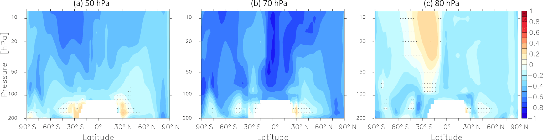
Figure 4Inter-model correlation coefficients for the correlation between RCTTs and tropical upwelling calculated at the turnaround latitudes (a) at 50 hPa, (b) at 70 hPa and (c) at 80 hPa. The stippled regions mark where the correlation is not significant on the 95 % confidence level.
We also address the question of whether simulated AoA (and thus CCM transport) improved in CCMI-1 compared to CCMVal-2. Eyring et al. (2006) analyzed CCMs from CCMVal-1 and reported that AoA in CCMVal-1 models is improved compared to previous model-data inter-comparisons. In the SPARC (2010) report, CCMs that participated both in CCMVal-1 and in CCMVal-2 were compared and no clear improvement in the simulation of AoA could be found. In our study the AoA performance for all analyzed CCMI-1 models that have a predecessor model in CCMVal-2, i.e., the models CMAM, MRI, GEOSCCM, SOCOL, ULAQ and WACCM (see Table 1) are examined (Fig. 3, dashed lines for CCMVal-2 and solid lines for CCMI-1). The AoA model spread is not reduced for the CCMI-1 REF-C1 simulations compared to the CCMVal-2 REF-B1 simulations. Additionally, we find that in most CCMI-1 models air is even younger than in their CCMVal-2 predecessor models (except for MRI, and tropical AoA values of SOCOL), and thus the simulations with the predecessor models agree better with observations. However, some forcings used in the CCMI-1 REF-C1 and the CCMVal-2 REF-B1 simulations are not identical. For example, one significant difference is the inclusion of an additional major volcanic injection of aerosol into the stratosphere in the CCMI-1 volcanic forcing dataset (see Morgenstern et al., 2017). This could explain the lower AoA in CCMI-1 REF-C1 simulations, as AoA in model simulations tends to be lowered by major volcanic eruptions at higher altitudes (30 hPa), as recently shown by Pitari et al. (2014). However, this also means that we cannot clearly separate the effect of differences in forcing and model improvement (e.g., higher resolution in CCMI-1 REF-C1 simulations).
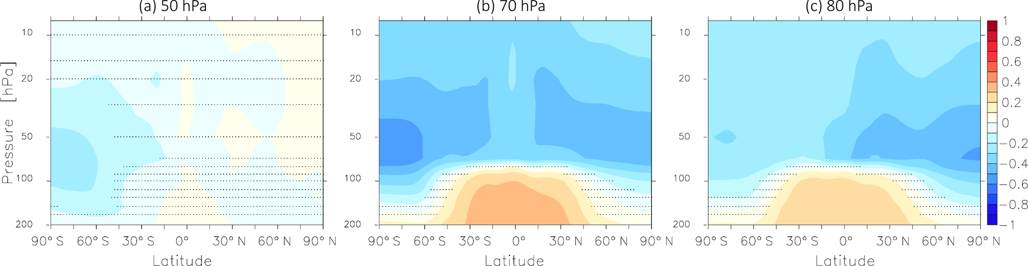
4.2 Inter-model correlation of tropical upwelling with RCTT and AoA
The residual circulation is often measured by the strength of tropical upwelling, commonly used at 70 hPa. In the following we investigate whether tropical upwelling is a good measure of the transport times along the residual circulation throughout the stratosphere. We calculate the inter-model correlation of annual mean climatologies of tropical upwelling at a certain level with the RCTTs across all 17 models. Tropical upwelling is averaged between the individual turnaround latitudes of each model, respectively. Note here that all correlations are quite robust, meaning that excluding the one or the other model from this analysis hardly changes the overall picture. Figure 4 shows the correlations between RCTTs and tropical upwelling at 80, 70 and 50 hPa. All panels in Fig. 4 mostly show negative correlations, which indicates that stronger tropical upwelling leads to reduced transit times through acceleration of the residual circulation (as expected from the dependence of RCTT on upwelling). The highest correlations can be found for tropical upwelling at 70 hPa. Here, the correlation reaches values above 0.8. These maxima can be found in the tropical pipe as well as in the downwelling branches of the BDC in the extratropics. The maximal correlation of tropical upwelling at 50 hPa with the RCTTs is found between 30 and 10 hPa and the structure resembles the deep BDC branch. The correlation with the tropical upwelling at 80 hPa is generally weaker and has its maxima in the lower extratropical stratosphere, i.e., in the region of the shallow branch of the BDC. Note that if we exclude the model LMDZrepro (which has a somewhat different RCTT pattern than other models, see Sect. 4.1), all these structures are even more pronounced in all three panels. These results indicate that tropical upwelling is a good measure of transport along the residual circulation, in particular at 70 hPa, while tropical upwelling above relates to transport in the deep branch and below to the shallow branch of the BDC.
Additionally, in Fig. 5, the correlations of tropical upwelling with AoA are shown. In general, the correlations of tropical upwelling with AoA are far weaker than for the RCTTs. The patterns seen in Fig. 4 are not visible here. Again, the highest correlations are found for tropical upwelling at 70 hPa with maxima reaching values around 0.5 in the extratropical lower stratosphere. For tropical upwelling at 50 hPa, hardly any correlation with AoA can be seen and tropical upwelling at 80 hPa only weakly correlates with AoA. As for the RCTTs, the strongest correlations are found in the extratropical lower stratosphere (only in the NH). Interestingly, in particular in the tropical pipe, correlations are lower compared to the extratropics (see 70 hPa tropical upwelling). This indicates that additional processes that act locally on AoA in the tropics play a role here, as for example tropical vertical diffusion. The comparably low correlations of tropical upwelling to AoA among all models show that mixing in general plays an important role for the simulation of AoA and that its relative effect on AoA varies in strength in different models. A more quantitative contribution of AoA to RCTTs and mixing follows in Sect. 4.3.
4.3 Mixing efficiency
In Sect. 4.1, we showed that AoA is influenced by the residual circulation and by mixing. However, these two processes are not independent, as both are linked to wave forcing (e.g., Garny et al., 2014). Furthermore, aging by mixing depends on the speed of recirculation, so that a stronger residual circulation also leads to lower aging by mixing, even if the strength of mixing itself does not change. To get a more independent measure of the mixing strength, we use the mixing efficiency ϵ. This measure is proportional to the relative increase in AoA due to mixing (i.e , see Eq. 1). Thus, ϵ=0 refers to no mixing (and AoA = RCTT) and increasing values of ϵ refer to an increase in relative mixing strength. The original definition of the mixing efficiency stems from the theoretical concept of the TLP model (see Sect. 3.2), where the mixing efficiency is defined as the ratio of the mixing mass flux to the net mass flux across the tropical barrier. However, in this formulation of the TLP model, vertical mixing or diffusion is neglected. Any numerical or parameterized diffusion both horizontally and vertically will influence tracer transport in the global model. The mixing efficiency calculated from the AoA fields of the models should therefore be interpreted as a measure of the relative enhancement of AoA by any mixing or diffusion.
Table 2 lists the derived mixing efficiencies for all model simulations. For the individual CCMVal-2 models the mixing efficiency varies between 0.24 (CMAM) and 1.02 (UMUKCA-METO). Note that the mixing efficiency of UMUKCA-METO lies far outside the typical range of the other models' mixing efficiency (from about 0.24 to 0.47). The CCMVal-2 multi-model mean of ϵ is 0.38 with a standard deviation of 32 % (see Table 3, first column). Note, however, that for calculating this multi-model mean UMUKCA-METO is excluded. For the CCMI-1 models the spread in mixing efficiency ranges from 0.28 (CMAM, WACCM) to 0.55 (MRI). The multi-model mean of the CCMI-1 model mixing efficiency of 0.36 is similar to that of the CCMVal-2 models. The standard deviation of 26 %, however, is somewhat smaller (see Table 3, first column). Taking into account all models together (CCMVal-2 and CCMI-1), the mean mixing efficiency is 0.37 with a standard deviation of 26 %. Sensitivity experiments with TLP calculations for two different tropical pipe definitions (i.e 30∘ N–30∘ S and turnaround latitudes) were conducted. These sensitivity experiments show that the variation in mixing efficiency does not decrease when using the model's individual turnaround latitudes (see Table 3, second and third column). Thus, it can be concluded that the large differences in ϵ between models cannot be explained by the fact that the various models have different widths of the tropical band.
Table 2Mixing efficiency ϵ for all CCMVal-2 REF-B1 (left) and CCMI-1 REF-C1 (right) simulations used in this study. ϵ is derived from the TLP model, with the border of the tropical pipe ranging between 20∘ N and 20∘ S.
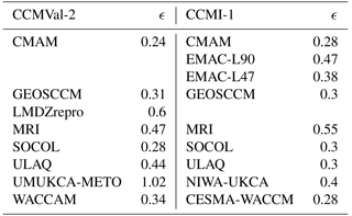
Table 3CCMVal-2 REF-B1 and the CCMI-1 REF-C1 multi-model mean of mixing efficiency ϵ and its 1σ inter-model standard deviation (in %). ϵ is derived by the TLP model, using three different tropical pipe definitions: 20∘ S–20∘ N, 30∘ S–30∘ N, and turnaround latitudes (TR). Note that the multi-model means of ϵ exclude the models UMUKCA-METO (CCMVal-2).
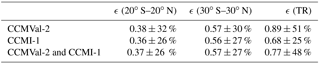

Figure 6Scatterplot showing the relationship between mean tropical (20∘ N–20∘ S) AoA and (a) mean tropical RCTT and (b) mixing efficiency. CCMVal-2 models are represented by cross symbols and CCMI-1 models by filled dots, except EMAC-L47, which is represented by a triangle. Values are all given at 10 km above the tropical tropopause. The corresponding correlation coefficients R are given within the individual panels.
The large CCMVal-2 and CCMI-1 model spreads in ϵ indicate that the relative mixing strength (i.e., the amount of any kind of mixing relative to the strength of the residual circulation) varies strongly among the different models or, in other words, mixing leads to different magnitudes in the relative enhancement of AoA.
Figure 6 shows the relationship between tropical AoA and tropical RCTT (Fig. 6a) and between tropical AoA and mixing efficiency (Fig. 6b) for all analyzed CCMVal-2 (crosses) and CCMI-1 (dots) models. Tropical values are all averaged over 20∘ N–20∘ S and are given at 10 km above the tropopause (corresponding to approximately 20 hPa).
As shown in Fig. 6a, tropical AoA is poorly correlated with tropical RCTT. The correlation coefficient for CCMVal-2 models is only 0.15 (increases to 0.66 when neglecting the outlier model UMUKCA-METO). For the CCMI-1 models the correlation is 0.29 (see Fig. 6a), and for all models (CCMVal-2 and CCMI-1) the correlation is 0.21. However, neglecting the outlier model UMUKCA-METO, the correlation increases to 0.47 for all models. Thus, the differences in AoA between the models can be explained only to some degree by differences in the strength of the residual circulation. In contrast, a high correlation is found between the tropical AoA and the mixing efficiency (Fig. 6b) with a correlation coefficient of 0.85 for CCMVal-2, of 0.82 for CCMI-1 and of 0.85 for all analyzed models. Note here that excluding again the outlier model UMUKCA-METO does decrease the correlation coefficient of all models to 0.63. The relation of tropical AoA to RCTT and the mixing efficiency is shown here for 10 km above the tropopause, but the result of the strong relation of AoA to the mixing efficiency and the weak relation of AoA to RCTT holds for all heights (not shown here). We conclude that the differences in the mixing efficiency between the models can explain large parts of the spread in simulated AoA. For example, for the outlier model UMUKCA-METO the very high AoA value can be explained with a very high mixing efficiency of 1.02, while the RCTT of UMUKCA-METO lies in the same range as other models (see Fig. 6a). Thus, it is not a particularly slow circulation that leads to high AoA in UMUKCA-METO, but relatively large mixing.
Further, we compare CCMI-1 models with their CCMVal-2 predecessor models to analyze if there is a systematic change with respect to mixing efficiency in the more recent CCMI-1 simulations. Table 2 shows that ϵ changes from CCMVal-2 to CCMI-1 are very small (< 2 %) for GEOSCCM and SOCOL and minor (< 15 %) for CMAM, MRI and WACCM. Two models show a significant change in ϵ from CCMVal-2 to CCMI-1: in ULAQ, the mixing efficiency decreases from 0.44 to 0.3 and in the UKCA model from 1.02 to 0.4. Thus, in both cases the mixing efficiency lies closer to the multi-model mean in CCMI-1. Reasons for this will be discussed in the Sect. 5.2.
In the last section, we showed that differences in the simulation of AoA in different models are strongly determined by differences in the mixing efficiency, i.e., the relative enhancement of AoA by any mixing processes in the model. In the formulation of the TLP model, the mixing efficiency is defined as the relative strength of horizontal mixing between the up- and downwelling regions. An independent measure of the relative role of horizontal mixing and mean transport is the ratio of mean potential vorticity (PV) to the meridional PV gradient (dPVdy). Details for the calculation of the PV gradients diagnostic are given in Garny et al. (2014). The spread of mixing efficiencies across the models is, however, only weakly correlated to the PV gradient diagnostic with the highest correlations found in midlatitudes at 450 K and correlation coefficients of about 0.5 (not shown). This weak correlation indicates that processes other than horizontal mixing play an important role in determining the mixing efficiency. In the following we present a detailed discussion of the possible effects of different processes on the mixing efficiency.
In Sect. 5.1 we will focus on the impact of vertical dispersion and in Sect. 5.2 on the impact of model-dependent representations of numerics (e.g., advection scheme and resolution) and dynamics (unresolved wave forcing).

Figure 7(a) Tropical mean (20∘ N–20∘ S) vertical residual velocities (black dashed) from one model (EMAC-L90) and effective tropical velocities derived from the tropics-to-midlatitude age difference in EMAC-L90 (black solid), in a TLP model driven by vertical velocities from EMAC-L90 and without diffusion (gray), with vertical diffusion of K=0.2 m2 s−1 in the tropics (green) and the extratropics (red). (b) Tropical (20∘ N–20∘ S) AoA profiles from EMAC-L90 (black solid) together with AoA profiles simulated by a TLP model with no vertical diffusion (gray line, identical to analytical TLP solution used to derive the mixing efficiencies), with vertical diffusion of K=0.2 m2 s−1 in the tropics (green) and the extratropics (red). (c) Same as (b) but for midlatitude AoA profiles (35–45∘ N and 35–45∘ S). (d) Difference between midlatitude and tropical AoA profiles.
5.1 Impact of vertical dispersion on AoA profiles
According to the TLP model formulation, the age difference between tropics and midlatitudes (ΔAoA) is a function of the tropical vertical velocity (w∗), but independent of horizontal mixing (Neu and Plumb, 1999): . Tropical means are calculated over 20∘ N–20∘ S and extratropical means over 35–45∘ N and 35–45∘ S. This solution is only valid when vertical diffusion is neglected. As this is not necessarily a good assumption, the vertical velocity calculated from the AoA difference will be a tracer-dependent effective vertical velocity in the tropics (weff). “Effective” refers to the effective vertical transport of the regarded tracer (i.e., AoA) that is consistent with the TLP model.
The effective vertical velocities calculated from age differences (AoA difference see Fig. 7d) from one model (EMAC-L90) are compared to the actual tropical mean residual vertical velocity (w∗) in Fig. 7a. In particular in the lower stratosphere, the effective vertical velocity (black line) calculated from the age difference overestimates the actual vertical velocity w∗ (black dashed line). Note that, in all the models analyzed in this study, the effective vertical velocity is similar to or larger than w∗ (not shown), as was also shown for the CCMVal-2 models in SPARC (2010) (their Fig. 5.6).
Vertical diffusion (or more generally, any process causing vertical dispersion) reduces the AoA difference. As discussed in Neu and Plumb (1999) and in Linz et al. (2016) (for isentropic coordinates). In the following, the TLP model is modified by including vertical diffusion (calculated as a Lagrangian random walk model, see Sect. 3.2). Figure 7b and c show tropical and midlatitude AoA profiles simulated with the TLP model given the vertical velocity profiles from one CCM (EMAC-L90). Profiles are given in height coordinates above the tropical mean tropopause. The Lagrangian TLP model without diffusion (K=0, gray line) reproduces the analytical solution of the TLP model (mixing efficiency as estimated with the method described above). The tropical AoA profile from the TLP model is close to the AoA profile from the full CCM (black line), but the midlatitude AoA of the CCM is overestimated by the TLP model without diffusion between 0 and 8 km above the tropical tropopause.
Introducing vertical diffusion in the extratropics (KML=0.2 m2 s−1) in the TLP model reduces extratropical AoA in the region of 0–8 km above the tropopause (red line) and weakly influences tropical AoA. Tropical vertical diffusion (with vertical diffusivity KTr=0.2 m2 s−1) leads to younger air in the tropics, and this signal is propagated into the midlatitudes (green line). Adding vertical diffusion in both regions (K=0.2 m2 s−1) combines the effects of tropical and extratropical vertical diffusion (not shown). The effective vertical velocities derived from the TLP model with extratropical diffusion roughly match the effective vertical velocities from the CCM (see black and red line in Fig. 7a). This simple experiment with the TLP model thus indicates that the deviations of the effective vertical velocities (derived from age gradients) from w∗ can be explained by vertical dispersion, which in particular leads to a reduced vertical age gradient in the extratropical lower stratosphere. The differences between the weff and w∗ varies across models (not shown); i.e., in some models AoA is more strongly modified by vertical dispersion than in others. In the simplified and conceptual TLP model, a constant vertical diffusivity was prescribed to illustrate the effects of any processes that act like vertical diffusion have on the AoA profile. In the full CCMs, a number of processes might contribute to the vertical dispersion. In most models, the vertical resolution is high enough to resolve some gravity waves (or mixed Rossby-gravity waves), which lead to resolved vertical dispersion. Furthermore, as we use (log-)p coordinates, adiabatic mixing is partly projected to the vertical axis. Nevertheless, diffusion due to unresolved processes and numerical diffusion (see also next section) contribute to varying degrees of vertical dispersion. Linz et al. (2016) estimate a lower stratospheric diffusivity of K=0.1 m2 s−1 based on isentropic coordinate diagnostics. This value is consistent with earlier estimates (e.g., Sparling et al., 1997). However, it is important to note that some vertical mixing is quasi-adiabatic and therefore implicitly included in isentropic (adiabatic) coordinates. Glanville and Birner (2017) find a much enhanced contribution to lower stratospheric water vapor transport due to vertical diffusion in pressure coordinates.
From the discussion of the effects of vertical dispersion on AoA, the following conclusions can be drawn: (1) the AoA difference is a biased measure of the tropical vertical residual circulation velocities in the lower stratosphere, or, in other words, vertical dispersion cannot be neglected. At higher altitudes (above about 10 km above the tropical tropopause, i.e., about 26 km or 30 hPa) the age difference is a better measure of tropical residual circulation velocities. This result is in agreement with Linz et al. (2016). (2) The mixing efficiencies derived for the models will bear non-negligible information of vertical dispersion and are not necessarily good measures of the relative strength of horizontal mixing. As the strength of vertical dispersion differs from model to model and thus has varying influence on the mixing efficiency, the spread in the mixing efficiencies across models cannot be related to differences in horizontal mixing alone (i.e., the correlation to the PV gradient diagnostic is weak, see above).
When calculating mixing efficiencies based on the effective vertical velocities (that include the effects of vertical dispersion), the spread in those modified mixing efficiencies relates better to horizontal mixing as measured by the PV diagnostic (with a correlation coefficient of about 0.77 at 450 K in midlatitudes), as the effective vertical velocities implicitly include the effects of vertical dispersion.
In other words, the mixing efficiency diagnosed from w∗ is a measure of the overall effects of both horizontal and vertical mixing.
5.2 Model characteristics that can influence mixing
In this section, we discuss dynamical and numerical model characteristics which have the potential to influence horizontal, vertical and numerical mixing. First, we analyze the possible role of the models' dynamics on horizontal mixing. As mentioned above, the dissipation of wave energy in the stratosphere largely controls the BDC. This wave energy comes from resolved planetary and synoptic waves as well as from unresolved gravity waves. Butchart et al. (2011) found an approximate ratio of 70 % EPFD and 30 % GWD (20 % NOGWD and 10 % OGWD) that drives tropical upwelling at 70 hPa in the CCMVal-2 models. However, this ratio differs largely between various models. Cohen et al. (2013) suggest that due to compensation effects between the different wave types, the impact of the differences in gravity wave perturbation on the total circulation is reduced. Hence, models tend to agree more on the total strength of the circulation than on individual components. Mixing, however, is influenced differently through the two wave types. Rossby-wave breaking predominately causes mixing and stirring in the horizontal, while dissipation of gravity waves mainly leads to vertical mixing. Furthermore, gravity waves are parameterized in the models, and effects of mixing on tracers are usually not explicitly included in the parameterizations. Thus, while all wave types drive residual transport, GWs do not cause horizontal mixing in the same way as resolved waves do.
A resulting hypothesis is that the ratio of Rossby-wave forcing to overall wave forcing influences the strength of horizontal mixing and thus the mixing efficiency. This means that the models' ratios between EPFD and total wave forcing (EPFD+GWD) could be related to their mixing efficiencies, which could at least partly explain the AoA differences between the models.
Figure 8 shows the climatological ratio of resolved wave drag divided by the total wave drag between 100 and 10 hPa for the CCMVal-2 REF-B1 and for the CCMI-1 REF-C1 simulations. Note that compared to the previous sections, fewer models are included in this analysis because the EPFD and GWD data are not provided for all models. In the lower stratosphere, all models indicate the strongest GWD contribution (low ratios); thus, gravity wave forcing has the strongest contribution by the overall forcing of the residual circulation in the analyzed height range. Towards higher altitudes (10 hPa), the impact of gravity waves decreases, before it increases again strongly above 1 hPa (not shown). Three models are presented twice in the figure, once each for the CCMI-1 and CCMVal-2 simulations. The EMAC model is also presented twice, but once for the simulation with 90 layers in the vertical and once with 47 layers. The two CMAM simulations show very similar wave-type ratios, the two GEOSCCM simulations have a similar vertical structure, but with an offset. The MRI simulations differ vastly. Note that in both model inter-comparison projects the same gravity wave parameterization schemes have been used in the respective models. The vertically higher resolved EMAC model has a more compact region of low wave-type ratio in the lower stratosphere but otherwise the two simulations show similar results.
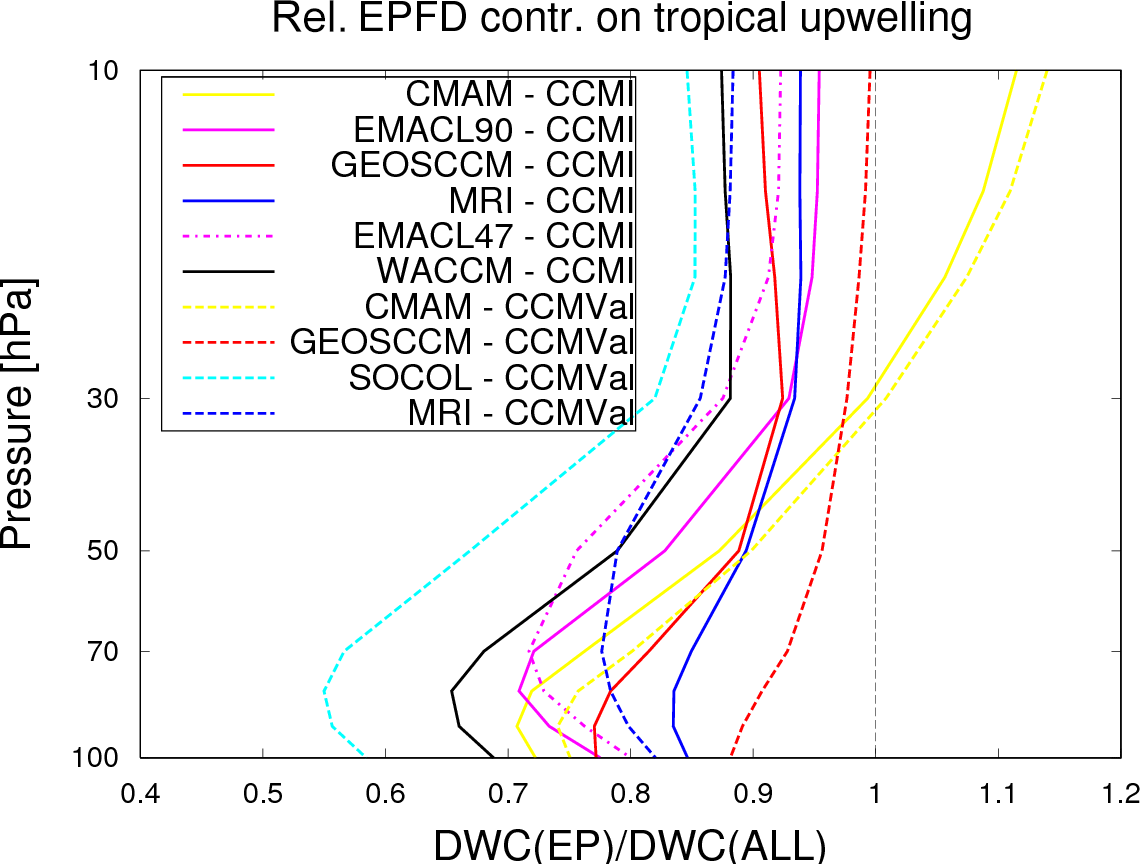
Figure 8Relative EPFD contribution on tropical upwelling (calculated as EPFD contribution of downward control calculated tropical upwelling divided by overall tropical upwelling) 30∘ N–30∘ S as function of pressure for all CCMVal-2 and CCMI-1 models providing the data for this analysis.
In general, the wave-type ratios of the different models show a considerable spread. At 70 hPa for example, it ranges from around 0.55 in the SOCOL (CCMVal-2) simulation to around 0.9 in the GEOSCCM (CCMVal-2) simulation.
As explained above, a larger ratio of resolved to parameterized wave forcing in the region where wave breaking leads to transport across the subtropical barrier causes stronger horizontal mixing and, therefore, leads to additional aging by mixing of stratospheric air. However, we found no clear correlation (ranging from 0.2 to 0.53 depending on altitude) between the wave-type ratio and the mixing efficiency throughout this altitude range. The hypothesis that differences in mixing efficiency can be explained by differences in wave driving therefore has to be rejected. For two of the three models that appear twice in the statistics (CMAM and GEOSCCM), the mixing efficiency increases while the EPFD wave-type ratio decreases from one model version to another. This behavior also stands in contrast to our possible physical explanation. Rossby waves can have a strengthening or weakening effect on the subtropical transport barrier depending on latitude and height of their location of dissipation. This may be the reason why the wave-type ratio is apparently not a good measure for the mixing between tropics and extratropics. However, the sample size of the available data is too small to statistically draw robust conclusions, so more data could possibly still impact the results. As for now, however, this attempt does not explain the potential to help explaining the AoA differences between the models.
As discussed in detail in Sect. 5.1 vertical mixing and diffusion (both resolved and unresolved) influences AoA (and thus the mixing efficiency). Furthermore, numerical diffusion can also influence horizontal mixing. Dietmüller et al. (2017) presented a method to separate resolved and unresolved mixing (including both vertical and horizontal unresolved mixing) by explicitly calculating the contribution of subgrid-scale mixing to aging by mixing (termed aging by diffusion). Their study showed that aging by diffusion is positive in most regions, indicating that horizontal diffusion dominates (as vertical diffusion would lead to a reduction in AoA). The calculation as performed in Dietmüller et al. (2017) requires the full four-dimensional fields of dynamical quantities and AoA, which were not available for the CCMVal-2 and CCMI-1 models. Therefore, we can only discuss the possible differences in subgrid-scale mixing between the models qualitatively. The two factors that most likely contribute to subgrid-scale mixing are the advection scheme and the horizontal and vertical resolution.
First we discuss the possible role of the model's advection schemes (see Table 1). The study of Eluszkiewicz et al. (2000) showed that AoA is very sensitive to the advection scheme used to integrate the tracer continuity equation. Semi-Lagrangian schemes are overly diffusive, whereas the finite volume and flux-form schemes are more accurate. However, the more recent study of Eyring et al. (2006) showed only small differences in AoA between spectral and flux-form advection schemes; thus, errors associated with spectral advection do not accumulate (Shepherd, 2007). Linking the mixing efficiency obtained for the CCMVal-2 and CCMI-1 models to their advection scheme, we find that ϵ for more accurate advection schemes (FFSL, FFEE) ranges from 0.28 to 0.47 and for more diffusive advection schemes (SP and SL) from 0.24 to 0.55 (1.02 UMUKCA-METO). SOCOL changed the advection scheme from SL in CCMVal-2 to FFSL in CCMI-1 with nearly no effect on ϵ. Thus, based on this sample, we cannot find a clear systematic relationship between ϵ and different advection schemes; however, the simple size is very small. Moreover, models can use the same advection scheme, but with additional explicit diffusion, or in SL schemes higher order interpolation is possible; thus, the model's advective transport can differ although using the same type of advection scheme. For example, the UMUKCA-METO model and its predecessor model NIWA-UKCA both use the same SL advection scheme, but with different polynomial interpolation. The CCMI model NIWA-UKCA used optimized settings governing transport and advection by a higher order of interpolation. This likely strongly reduces horizontal numerical diffusion and thus leads to lower AoA (and smaller ϵ) in NIWA-UKCA.
Second, we address whether the increase in spatial resolution, which is apparent for many CCMs since CCMVal-2 (see the models' horizontal and vertical resolution in Table 1), has an impact on the mixing efficiency. Rind et al. (2007) showed that horizontal resolution (truncation error) has little impact on AoA, whereas a fine vertical resolution leads to higher AoA throughout the stratosphere. Faster inter-hemispheric transport and slower mixing into and out of the stratosphere cause this behavior. The models CMAM, MRI, SOCOL and ULAQ have increased their horizontal resolution since CCMVal-2, and the models MRI and ULAQ have also increased their vertical resolution. The ULAQ model is the only model that substantially changed vertical and horizontal resolution (see Table 1). The coarse resolution (in particular very low horizontal resolution) in the ULAQ REF-B1 simulation indicates that the transport barriers at the edge of the tropics and at the polar vortex are likely not reproduced very well (see also SPARC, 2010). The quite-large mixing efficiency of 0.44 in CCMVal-2 is now closer to the multi-model mean with the higher resolution in CCMI-1 (to 0.3). The fact that ULAQ AoA in CCMVal-2 was in a similar range as the other models might well be due to compensation effects of vertical and horizontal numerical diffusion on AoA. This hypothesis is also supported by the PV gradient of ULAQ CCMVal-2 simulation, which lies far outside of the model range (figure not shown here). Regarding the two EMAC simulations within CCMI-1 with differing vertical resolution, the version with higher vertical resolution has a higher AoA (see Fig. 2), as expected from less vertical diffusion. A similar result was obtained for SOCOL sensitivity simulations (Revell et al., 2015 and Andrea Stenke, personal communication, 2017). The mixing efficiency in the EMAC simulation with lower resolution is reduced compared to the higher resolved model (mixing efficiency 0.47 for EMAC-L90 vs. 0.38 for EMAC-L47), likely due to enhanced vertical numerical diffusion.
In general the results presented here suggest that the vertical resolution affects AoA and mixing efficiency, as seen in the EMAC and SOCOL sensitivity simulations and also for the ULAQ model. However, except ULAQ, the only model that changed vertical resolution from CCMVal-2 to CCMI is MRI; all other models only have changes in the horizontal resolution, where at this high resolution the models used might not play a big role (in agreement with Rind et al., 2007). For all other models with smaller changes in resolution than in ULAQ, no clear effect on the mixing efficiency could be detected.
The various factors that likely influence a model's subgrid mixing or diffusion are hard to disentangle for the given set of models. Additional sensitivity studies with one given model would be necessary to analyze the role of the different factors (i.e., advection scheme, horizontal and vertical resolution).
This study analyzes the climatological AoA of various stratosphere-resolving CCMs, which participated in the model inter-comparison projects CCMVal-2 and CCMI-1, in order to investigate the causes of the differences in AoA among the models. We showed that the tropical and midlatitude AoA profiles of most examined models have younger air compared to observations, but most AoA profiles lie within the uncertainty of values derived from observations. Moreover, there is a large spread in the simulated AoA between models. This result is in agreement with earlier model comparison studies (e.g., Eyring et al., 2006; SPARC, 2010). We could not detect an improvement in the simulation of AoA from CCMI-1 models compared to CCMVal-2. The CCMI-1 models tend to simulate younger air compared to their predecessor models. However, an exact one-by-one comparison is not possible because the forcings used in the CCMVal-2 and CCMI-1 hindcast simulations are not identical.
To better understand the AoA model differences, we investigated the processes that affect stratospheric transport and thus AoA. Both transport by the residual circulation and aging by mixing influence the zonal structure and magnitude of AoA. Models agree on the zonal pattern of residual transport and aging by mixing, with mixing leading to additional aging in most of the stratosphere in all model simulations. Also the high inter-model correlation between tropical upwelling and RCTTs and the low correlation between tropical upwelling and AoA indicate that mixing plays an important role in the simulation of AoA. The strength of tropical-to-midlatitude mixing relative to residual transport is measured by the mixing efficiency, a quantity that can be calculated from model data given the tropical mean AoA profile and tropical vertical residual velocities. The mixing efficiency is a measure of the relative aging by mixing in a model, which is independent of the strength of the residual circulation, and it varies strongly between models. However, the mixing efficiency measures the overall effects of mixing, as it accounts for both horizontal and vertical mixing and both resolved and unresolved mixing. We showed with the help of the Lagrangian TLP model that vertical diffusion has a significant impact on the mixing efficiency and thereby on the structure of AoA. The consequence of this is that the mixing efficiency is not necessarily a good measure of the relative strength of horizontal mixing alone.
We showed that the model spread in the simulation of AoA is mostly caused by large differences in the mixing efficiency, because the inter-model correlation coefficient of mixing efficiency with AoA is higher (0.85/0.67 with/without outlier model) compared to the correlation with residual transport: the correlation of residual transport (RCTT) to AoA is quite low (inter-model correlation is 0.21/0.47 with/without outlier model). Thus, differences in the simulated residual circulation matter less to the simulated AoA compared to the relative mixing strength. We can conclude that analyzing the models' mixing efficiency is very useful for the understanding of their differences in AoA. The values of the mixing efficiency vary strongly, ranging between 0.24 and 1.02. The multi-model mean of the mixing efficiency of the CCMVal-2 REF-B1 simulations (ϵ=0.38) is similar to the one for the CCMI-1 REF-C1 simulations (ϵ=0.37), but the model spread in mixing efficiency is somewhat higher in the CCMVal-2 models (standard deviation of 32 % compared to 26 % in CCMI-1, without outliers).
In the SPARC CCMVal report the model performance on stratospheric transport diagnostics was qualitatively evaluated. CCMVal-2 models were graded (with grades indicating the agreement with observations) based on their mean AoA and on measures of tropical ascent and tropical–extratropical mixing derived from tracer diagnostics (see Table 5.1 in SPARC, 2010). The models with high grades in global mean AoA according to SPARC (2010) generally also were graded high in tropical ascent and mixing (see Fig. 5.19 in SPARC, 2010). It was also found that the grade of tropical ascent and mixing correlate quite strongly (see Fig. 5.20 in SPARC, 2010). This finding is somewhat opposed to our results, where a perfect relation between residual transport and mixing would lead to the same mixing efficiency for all CCMVal-2 and CCMI-1 models. However, first, the measures of tropical ascent and mixing in SPARC (2010) were based on tracers that did not perfectly separate the processes of mixing and residual circulation and, second, we expect a good relationship between residual transport and the absolute amount of mixing (as both are driven by wave driving), but the deviation from this relationship caused the differences in the relative mixing strength (i.e., the mixing efficiency). In general, models that were graded high in SPARC (2010) (namely CMAM, GEOSCCM, MRI, ULAQ and WACCM of CCMVal-2) were also found to have mixing efficiencies in the typical range (between 0.24 and 0.47) here. The models that obtained low grades in SPARC (2010) and that were analyzed here are SOCOL, with very young air, and UMUKCA-METO, with very old air. For SOCOL, we found that, next to fast tropical ascent, a quite-low mixing efficiency (0.3) also contributes to the young air. For the outlier model UMUKCA-METO, in SPARC (2010) slow tropical ascent and too-weak mixing was found. While weak mixing would lead to lower AoA, we show that mixing is strong relative to the residual circulation. Thus, we find that, on top of a slow circulation, a large mixing efficiency (ϵ=1.02) leads to the very old air in UMUKCA-METO. The comparison to the stratospheric transport diagnostics used in SPARC (2010) shows that using the diagnostic of the mixing efficiency provides additional information on the ability of a model to simulate stratospheric transport. We found that the relative strength of mixing in a model can mainly explain deficits in the simulation of AoA. However, a problem with the mixing efficiency diagnostic is the lack of observational constraints. It would be possible to define a mixing efficiency from the observational AoA profile and the vertical residual velocities estimated from the AoA gradients. However, those vertical velocities are substantially influenced by vertical diffusion and thus this mixing efficiency does not measure the same thing as the model-derived mixing efficiency. Thus, we cannot identify whether deficits in the absolute circulation and mixing strength or a too-strong or too-weak mixing efficiency are the cause for deviations in AoA from observations. Another problem might be that any errors in the calculation of AoA or RCTTs would be reflected in the mixing efficiency.
Within this study we also discussed the different dynamical and numerical model characteristics, which impact horizontal, vertical and numerical mixing. Besides vertical diffusion (Sect. 5.1), subgrid-scale mixing likely influences the mixing efficiency. This assumption motivates a closer look at the possible impact of the models' different advection schemes as well as horizontal and vertical resolution on sub-grid-scale mixing (Sect. 5.2). The results suggest that the vertical resolution affects AoA and mixing efficiency, as seen from EMAC and SOCOL sensitivity simulations with different vertical resolution (for EMAC the mixing efficiency increases from 0.38 to 0.47 with higher resolution; for SOCOL the sensitivity simulation was not available within CCMI-1). Moreover, for the ULAQ model a substantial increase in the resolution (both horizontal and vertical) between CCMVal-2 and CCMI-1 reduced the mixing efficiency (from 0.44 to 0.3). We did not find a systematic relationship between mixing efficiency and the models' different advection schemes. In general no systematic attribution of AoA differences to advection schemes or resolution could be made. This is because more than one parameter has been changed between the simulations. Furthermore, we demonstrated that the relative contribution of resolved versus parameterized wave forcing of the circulation is very different among the models. Since resolved Rossby-wave forcing induces strong horizontal mixing, parameterized GW forcing induces no mixing, and both drive the residual circulation; this might have an influence on the mixing efficiency. However, since the correlation of modeled wave-type ratio with the mixing efficiency is very low, the difference in models' resolved and parameterized waves does not explain the AoA differences. In conclusion, we can say that we found some evidence for the differences in mixing efficiency. However, overall, dedicated sensitivity studies with at least one given model system will be necessary to better determine the role of possible causes for the spread in the mixing efficiency (e.g., differences in resolution, advection scheme, GW drag).
Previous studies showed that within one model the mixing efficiency remains constant also in a changing climate (Garny et al., 2014). If this is true for all models, any changes in the residual circulation will be related linearly to changes in AoA (as also suggested by Austin and Li, 2006). The different values of the mixing efficiency in models would then modulate the relative increase in AoA by increasing the residual circulation. In a follow-up study, we will focus on AoA trends in the CCMVal-2 and CCMI-1 future change scenario simulations and investigate how the mixing efficiency in the analyzed models evolves in a changing climate, and possible processes for changes in the mixing efficiency will be discussed.
All data of CCMVal-2 and CCMI-1 used in this study can be obtained through the British Atmospheric Data Centre (BADC) archive (ftp://ftp.ceda.ac.uk, last access: June 2017). CESM1-WACCM data have been downloaded from http://www.earthsystemgrid.org (last access: June 2017). For instructions for access to both archives see http://blogs.reading.ac.uk/ccmi/badc-data-access. MIPAS data are available from https://www.imk-asf.kit.edu/english/308.php (last access: November 2017, after registration). AoA from GOZCARDS N2O are available under https://figshare.com/articles/NGeo2017_plots_m/5229844/1 (last access: February 2018).
The supplement related to this article is available online at: https://doi.org/10.5194/acp-18-6699-2018-supplement.
SD, RE and HG made substantial contributions to the conception and design, analysis and interpretation of the data. Moreover, they participated in drafting the article. TB and HB contributed to the discussion on the content and the structure of the paper. The other authors contributed information pertaining to their individual models and helped revise this paper.
The authors declare that they have no conflict of interest.
This article is part of the special issue “Chemistry–Climate Modelling Initiative (CCMI) (ACP/AMT/ESSD/GMD inter-journal SI)”. It is not associated with a conference.
This study was funded by the Helmholtz Association under grant VH-NG-1014
(Helmholtz-Hochschul-Nachwuchsforschergruppe MACClim).
We acknowledge the
modeling groups for making their simulations available for this analysis, the
WCRP SPARC Chemistry–Climate Model Validation (CCMVal) Activity and
the SPARC/IGAC Chemistry–Climate Model Initiative (CCMI) project for
organizing and coordinating the model data analysis activity, as well as the British
Atmospheric Data Centre (BADC) for collecting and archiving the CCMVal and
CCMI model output. Moreover, we want to acknowledge that the EMAC simulations
were done within the project ESCiMo (Earth System Chemistry integrated
Modelling), a national (German) contribution to the Chemistry–Climate Model
Initiative, and have been performed at the German Climate Computing Centre
DKRZ through support from the Bundesministerium für Bildung und Forschung
(BMBF). Moreover, we thank Florian Haenel and Gabriele Stiller for providing
us the MIPAS AoA data, Marianna Linz for providing us AoA from GOZCARDS
N2O data and also Andreas Engel for providing us the in situ tropical AoA
data.
The article processing charges for this open-access
publication
were covered by a Research
Centre of the Helmholtz Association.
Edited by: Andrew Gettelman
Reviewed by: Marianna Linz, Eric Ray, and one anonymous referee
Andrews, A. E., Boering, K. A., Daube, B. C., Wofsy, S. C., Loewenstein, M., Jost, H., Podolske, J. R., Webster, C. R., Herman, R. L., Scott, D. C., Flesch, G. J., Moyer, E. J., Elkins, J. W., Dutton, G. S., Hurst, D. F., Moore, F. L., Ray, E. A., Romashkin, P. A., and Strahan, S. E.: Mean ages of stratospheric air derived from in situ observations of CO2, CH4, and N2O, J. Geophys. Res.-Atmos., 106, 32295–32314, https://doi.org/10.1029/2001JD000465, 2001. a, b, c, d, e, f, g, h, i, j, k, l
Austin, J. and Li, F.: On the relationship between the strength of the Brewer-Dobson circulation and the age of stratospheric air, Geophys. Res. Lett., 33, L17807, https://doi.org/10.1029/2006GL026867, 2006. a
Birner, T. and Bönisch, H.: Residual circulation trajectories and transit times into the extratropical lowermost stratosphere, Atmos. Chem. Phys., 11, 817–827, https://doi.org/10.5194/acp-11-817-2011, 2011. a, b
Butchart, N.: The Brewer-Dobson circulation, Rev. Geophys., 52, 157–184, https://doi.org/10.1002/2013RG000448, 2014. a
Butchart, N., Cionni, I., Eyring, V., Shepherd, T., Waugh, D., Akiyoshi, H., Austin, J., Brühl, C., Chipperfield, M., Cordero, E., Dameris, M., Deckert, R., Dhomse, S., Frith, S., Garcia, R., Gettelman, A., Giorgetta, M., Kinnison, D., Li, F., Mancini, E., McLandress, C., Pawson, S., Pitari, G., Plummer, D., Rozanov, E., Sassi, F., Scinocca, J., Shibata, K., Steil, B., and Tian, W.: Chemistry-climate model simulations of twenty-first century stratospheric climate and circulation changes, J. Climate, 23, 5349–5374, 2010. a
Butchart, N., Charlton-Perez, A. J., Cionni, I., Hardiman, S. C., Haynes, P. H., Krüger, K., Kushner, P. J., Newman, P. A., Osprey, S. M., Perlwitz, J., Sigmond, M., Wang, L., Akiyoshi, H., Austin, J., Bekki, S., Baumgaertner, A., Braesicke, P., Brühl, C., Chipperfield, M., Dameris, M., Dhomse, S., Eyring, V., Garcia, R., Garny, H., Jöckel, P., Lamarque, J.-F., Marchand, M., Michou, M., Morgenstern, O., Nakamura, T., Pawson, S., Plummer, D., Pyle, J., Rozanov, E., Scinocca, J., Shepherd, T. G., Shibata, K., Smale, D., Teyssèdre, H., Tian, W., Waugh, D., and Yamashita, Y.: Multimodel climate and variability of the stratosphere, J. Geophys. Res.-Atmos., 116, 2156–2202, https://doi.org/10.1029/2010JD014995, 2011. a
Cohen, N. Y., Gerber, E. P., and Bühler, O.: Compensation between Resolved and Unresolved Wave Driving in the Stratosphere: Implications for Downward Control, J. Atmos. Sci., 70, 3780–2798, https://doi.org/10.1175/JAS-D-12-0346.1, 2013. a
Deushi, M. and Shibata, K.: Development of a Meteorological Research Institute chemistry-climate model version 2 for the study of tropospheric and stratospheric chemistry, Pap. Meteorol. Geophys., 62, 1–46, 2011. a
Dietmüller, S., Garny, H., Plöger, F., Jöckel, P., and Cai, D.: Effects of mixing on resolved and unresolved scales on stratospheric age of air, Atmos. Chem. Phys., 17, 7703–7719, https://doi.org/10.5194/acp-17-7703-2017, 2017. a, b, c, d, e
Eluszkiewicz, J., Hemler, R. S., Mahlman, J. D., Bruhwiler, L., and Takacs, L. L.: Sensitivity of age-of-air calculations to the choice of advection scheme, J. Atmos. Sci., 57, 3185–3201, 2000. a, b, c
Engel, A., Möbius, T., Bönisch, H., Schmidt, U., Heinz, R., Levin, I., Atlas, E., Aoki, S., Nakazawa, T., Sugawara, S., Moore, F., Hurst, D., Elkins, J., Schauffler, S., Andrews, A., and Boering, A.: Age of stratospheric air unchanged within uncertainties over the past 30 years, Nat. Geosci., 2, 28–31, 2009. a, b, c, d, e, f, g, h, i
Engel, A., Bönisch, H., Ullrich, M., Sitals, R., Membrive, O., Danis, F., and Crevoisier, C.: Mean age of stratospheric air derived from AirCore observations, Atmos. Chem. Phys., 17, 6825–6838, https://doi.org/10.5194/acp-17-6825-2017, 2017. a, b
Eyring, V., Butchart, N., Waugh, D. W., Akiyoshi, H., Austin, J., Bekki, S., Bodeker, G. E., Boville, B. A., Brühl, C., Chipperfield, M. P., Cordero, E. andls Dameris, M., Deushi, M., Fioletov, V. E., Frith, S. M., Garcia, R. R., Gettelman, A., Giorgetta, M. A., Grewe, V., Jourdain, L., Kinnison, D. E., Mancini, E., Manzini, E., Marchand, M., Marsh, D. R., Nagashima, T., Newman, P. A., Nielsen, J. E., Pawson, S., Pitari, G., Plummer, D. A., Rozanov, E., Schraner, M., Shepherd, T. G., Shibata, K., Stolarski, R. S., Struthers, H., Tian, W., and Yoshiki, M.: Assessment of temperature, trace species, and ozone in chemistry-climate model simulations of the recent past, J. Geophys. Res.-Atmos., 111, D22308, https://doi.org/10.1029/2006JD007327, 2006. a, b, c, d, e, f, g
Eyring, V., Lamarque, J.-F., Hess, P., Arfeuille, F., Bowman, K., Chipperfield, M., Duncan, B., Fiore, A., Gettelman, A., Giorgetta, M., Granier, C., Hegglin, M., Kinnison, D., Kunze, M., Langematz, U., Luo, B., Martin, R., Matthes, K., Newman, P., Peter, T., Robock, A., Ryerson, A., Saiz-Lopez, A., Salawitch, R., Schultz, M., Shepherd, T., Shindell, D., Stähelin, J., Tegtmeier, S., Thomason, L., Tilmes, S., Vernier, J.-P., Waugh, D., and Young, P.: Overview of IGAC/SPARC Chemistry-Climate Model Initiative (CCMI) Community Simulations in Support of Upcoming Ozone and Climate Assessments, SPARC newsletter, 40, 48–66, 2013. a, b
Froidevaux, L., Anderson, J., Wang, H.-J., Fuller, R. A., Schwartz, M. J., Santee, M. L., Livesey, N. J., Pumphrey, H. C., Bernath, P. F., Russell III, J. M., and McCormick, M. P.: Global OZone Chemistry And Related trace gas Data records for the Stratosphere (GOZCARDS): methodology and sample results with a focus on HCl, H2O, and O3, Atmos. Chem. Phys., 15, 10471–10507, https://doi.org/10.5194/acp-15-10471-2015, 2015. a
Garcia, R., Marsh, D., Kinnison, D., Boville, B., and Sassi, F.: Simulation of secular trends in the middle atmosphere, 1950–2003, J. Geophys. Res.-Atmos., 112, D09301, https://doi.org/10.1029/2006JD007485, 2007. a
Garcia, R. R., Smith, A. K., Kinnison, D. E., Cámara, Á. D. L., and Murphy, D. J.: Modification of the Gravity Wave Parameterization in the Whole Atmosphere Community Climate Model: Motivation and Results, J. Atmos. Sci., 74, 275–291, 2017. a
Garny, H., Birner, T., Bönisch, H., and Bunzel, F.: The effects of mixing on age of air, J. Geophys. Res.-Atmos., 119, 7015–7034, 2014. a, b, c, d, e, f, g, h, i, j, k, l, m, n, o, p
Ghoniem, A. F. and Sherman, F. S.: Grid-free simulation of diffusion using random walk methods, J. Comput. Phys., 61, 1–37, https://doi.org/10.1016/0021-9991(85)90058-0, 1985. a
Glanville, A. A. and Birner, T.: Role of vertical and horizontal mixing in the tape recorder signal near the tropical tropopause, Atmos. Chem. Phys., 17, 4337–4353, https://doi.org/10.5194/acp-17-4337-2017, 2017. a
Haenel, F. J., Stiller, G. P., von Clarmann, T., Funke, B., Eckert, E., Glatthor, N., Grabowski, U., Kellmann, S., Kiefer, M., Linden, A., and Reddmann, T.: Reassessment of MIPAS age of air trends and variability, Atmos. Chem. Phys., 15, 13161–13176, https://doi.org/10.5194/acp-15-13161-2015, 2015. a, b, c, d
Hall, T. M. and Plumb, R. A.: Age as a diagnostic of stratospheric transport, J. Geophys. Res.-Atmos., 99, 1059–1070, 1994. a, b, c, d
Hall, T. M., Waugh, D. W., Boering, K. A., and Plumb, R. A.: Evaluation of transport in stratospheric models, J. Geophys. Res.-Atmos., 104, 18815–18839, 1999. a
Haynes, P. and Shuckburgh, E.: Effective diffusivity as a diagnostic of atmospheric transport: 1. Stratosphere, J. Geophys. Res.-Atmos., 105, 22777–22794, https://doi.org/10.1029/2000JD900093, 2000. a
Haynes, P. H., McIntyre, M. E., Shepherd, T. G., Marks, C. J, and Shine K. P.: On the “Downward Control” of Extratropical Diabatic Circulations by Eddy-Induced Mean Zonal Forces, J. Atmos. Sci., 48, 651–678, https://doi.org/10.1175/1520-0469(1991)048<0651:OTCOED>2.0.CO;2, 1991. a
Holton, J. R., Haynes, P. H., McIntyre, M. E., Douglass, A. R., Rood, R. B., and Pfister, L.: Stratosphere-troposphere exchange, Rev. Geophys., 33, 403–439, https://doi.org/10.1029/95RG02097, 1995. a
Jöckel, P., Kerkweg, A., Pozzer, A., Sander, R., Tost, H., Riede, H., Baumgaertner, A., Gromov, S., and Kern, B.: Development cycle 2 of the Modular Earth Submodel System (MESSy2), Geosci. Model Dev., 3, 717–752, https://doi.org/10.5194/gmd-3-717-2010, 2010. a, b
Jöckel, P., Tost, H., Pozzer, A., Kunze, M., Kirner, O., Brenninkmeijer, C. A. M., Brinkop, S., Cai, D. S., Dyroff, C., Eckstein, J., Frank, F., Garny, H., Gottschaldt, K.-D., Graf, P., Grewe, V., Kerkweg, A., Kern, B., Matthes, S., Mertens, M., Meul, S., Neumaier, M., Nützel, M., Oberländer-Hayn, S., Ruhnke, R., Runde, T., Sander, R., Scharffe, D., and Zahn, A.: Earth System Chemistry integrated Modelling (ESCiMo) with the Modular Earth Submodel System (MESSy) version 2.51, Geosci. Model Dev., 9, 1153–1200, https://doi.org/10.5194/gmd-9-1153-2016, 2016. a, b
Jonsson, A., De Grandpre, J., Fomichev, V., McConnell, J., and Beagley, S.: Doubled CO2-induced cooling in the middle atmosphere: Photochemical analysis of the ozone radiative feedback, J. Geophys. Res.-Atmos., 109, D24103, https://doi.org/10.1029/2004JD005093, 2004. a
Jourdain, L., Bekki, S., Lott, F., and Lefèvre, F.: The coupled chemistry-climate model LMDz-REPROBUS: description and evaluation of a transient simulation of the period 1980–1999, Ann. Geophys., 26, 1391–1413, https://doi.org/10.5194/angeo-26-1391-2008, 2008. a
Kovács, T., Feng, W., Totterdill, A., Plane, J. M. C., Dhomse, S., Gómez-Martín, J. C., Stiller, G. P., Haenel, F. J., Smith, C., Forster, P. M., García, R. R., Marsh, D. R., and Chipperfield, M. P.: Determination of the atmospheric lifetime and global warming potential of sulfur hexafluoride using a three-dimensional model, Atmos. Chem. Phys., 17, 883–898, https://doi.org/10.5194/acp-17-883-2017, 2017. a
Linz, M., Plumb, R. A., Gerber, E. P., and Sheshadri, A.: The Relationship between Age of Air and the Diabatic Circulation of the Stratosphere, J. Atmos. Sci., 73, 4507–4518, https://doi.org/10.1175/JAS-D-16-0125.1, 2016. a, b, c
Linz, M., Plumb, R. A., Gerber, E. P., Haenel, F. J., Stiller, G., Kinnison, D. E., Ming, A., and Neu, J. L.: The strength of the meridional overturning circulation of the stratosphere, Nat. Geosci., 10, 663–667, https://doi.org/10.1038/ngeo3013, 2017. a, b
Marsh, D. R., Mills, M. J., Kinnison, D. E., Lamarque, J.-F., Calvo, N., and Polvani, L. M.: Climate change from 1850 to 2005 simulated in CESM1 (WACCM), J. Climate, 26, 7372–7391, 2013. a
Molod, A., Takacs, L., Suarez, M., Bacmeister, J., Song, I.-S., and Eichmann, A.: The GEOS-5 atmospheric general circulation model: Mean climate and development from MERRA to Fortuna, NASA Technical Report Series on Global Modeling Data Assimilation, NASA TM-2012-104606, 28, Greenbelt, MD, USA, 117 pp., 2012. a
Molod, A., Takacs, L., Suarez, M., and Bacmeister, J.: Development of the GEOS-5 atmospheric general circulation model: evolution from MERRA to MERRA2, Geosci. Model Dev., 8, 1339–1356, https://doi.org/10.5194/gmd-8-1339-2015, 2015. a
Morgenstern, O., Braesicke, P., O'Connor, F. M., Bushell, A. C., Johnson, C. E., Osprey, S. M., and Pyle, J. A.: Evaluation of the new UKCA climate-composition model – Part 1: The stratosphere, Geosci. Model Dev., 2, 43–57, https://doi.org/10.5194/gmd-2-43-2009, 2009. a, b, c
Morgenstern, O., Giorgetta, M., Shibata, K., Eyring, V., Waugh, D., Shepherd, T., Akiyoshi, H., Austin, J., Baumgaertner, A., Bekki, S., et al.: Review of the formulation of present-generation stratospheric chemistry-climate models and associated external forcings, J. Geophys. Res., 115, D00M02, https://doi.org/10.1029/2009JD013728, 2010. a, b, c, d, e, f, g
Morgenstern, O., Zeng, G., Luke Abraham, N., Telford, P. J., Braesicke, P., Pyle, J. A., Hardiman, S. C., O'Connor, F. M., and Johnson, C. E.: Impacts of climate change, ozone recovery, and increasing methane on surface ozone and the tropospheric oxidizing capacity, J. Geophys. Res.-Atmos., 118, 1028–1041, 2013. a, b
Morgenstern, O., Hegglin, M. I., Rozanov, E., O'Connor, F. M., Abraham, N. L., Akiyoshi, H., Archibald, A. T., Bekki, S., Butchart, N., Chipperfield, M. P., Deushi, M., Dhomse, S. S., Garcia, R. R., Hardiman, S. C., Horowitz, L. W., Jöckel, P., Josse, B., Kinnison, D., Lin, M., Mancini, E., Manyin, M. E., Marchand, M., Marécal, V., Michou, M., Oman, L. D., Pitari, G., Plummer, D. A., Revell, L. E., Saint-Martin, D., Schofield, R., Stenke, A., Stone, K., Sudo, K., Tanaka, T. Y., Tilmes, S., Yamashita, Y., Yoshida, K., and Zeng, G.: Review of the global models used within phase 1 of the Chemistry–Climate Model Initiative (CCMI), Geosci. Model Dev., 10, 639–671, https://doi.org/10.5194/gmd-10-639-2017, 2017. a, b, c, d, e, f
Nakamura, N.: Two-dimensional mixing, edge formation, and permeability diagnosed in an area coordinate, J. Atmos. Sci., 53, 1524–1537, 1996. a
Neu, J. L. and Plumb, R. A.: Age of air in a leaky pipe model of stratospheric transport, J. Geophys. Res.-Atmos., 104, 19243–19255, 1999. a, b, c, d, e, f
Newman, P. A., Schoeberl, M. R., and Plumb, R. A.: Horizontal mixing coefficients for two-dimensional chemical models calculated from National Meteorological Center data, J. Geophys. Res.-Atmos., 91, 7919–7924, https://doi.org/10.1029/JD091iD07p07919, 1986. a
Oman, L., Ziemke, J., Douglass, A., Waugh, D., Lang, C., Rodriguez, J., and Nielsen, J.: The response of tropical tropospheric ozone to ENSO, Geophys. Res. Lett., 38, L13706, https://doi.org/10.1029/2011GL047865, 2011. a
Oman, L. D., Douglass, A. R., Ziemke, J. R., Rodriguez, J. M., Waugh, D. W., and Nielsen, J. E.: The ozone response to ENSO in Aura satellite measurements and a chemistry-climate simulation, J. Geophys. Res.-Atmos., 118, 965–976, 2013. a
Pawson, S., Stolarski, R. S., Douglass, A. R., Newman, P. A., Nielsen, J. E., Frith, S. M., and Gupta, M. L.: Goddard Earth Observing System chemistry-climate model simulations of stratospheric ozone-temperature coupling between 1950 and 2005, J. Geophys. Res.-Atmos., 113, D12103, https://doi.org/10.1029/2007JD009511, 2008. a
Pitari, G., Mancini, E., Rizi, V., and Shindell, D.: Impact of future climate and emission changes on stratospheric aerosols and ozone, J. Atmos. Sci., 59, 414–440, 2002. a
Pitari, G., Aquila, V., Kravitz, B., Robock, A., Watanabe, S., Cionni, I., Luca, N. D., Genova, G. D., Mancini, E., and Tilmes, S.: Stratospheric ozone response to sulfate geoengineering: Results from the Geoengineering Model Intercomparison Project (GeoMIP), J. Geophys. Res.-Atmos., 119, 2629–2653, 2014. a, b
Ploeger, F., Abalos, M., Birner, T., Konopka, P., Legras, B., Müller, R., and Riese, M.: Quantifying the effects of mixing and residual circulation on trends of stratospheric mean age of air, Geophys. Res. Lett., 42, 2047–2054, https://doi.org/10.1002/2014GL062927, 2015a. a
Ploeger, F., Riese, M., Haenel, F., Konopka, P., Müller, R., and Stiller, G.: Variability of stratospheric mean age of air and of the local effects of residual circulation and eddy mixing, J. Geophys. Res.-Atmos., 120, 716–733, https://doi.org/10.1002/2014JD022468, 2015b. a, b, c
Ray, E. A., Moore, F. L., Rosenlof, K. H., Davis, S. M., Boenisch, H., Morgenstern, O., Smale, D., Rozanov, E., Hegglin, M., Pitari, G., Mancini, E., Braesicke, P., Butchart, N., Hardiman, S., Li, F., Shibata, K., and Plummer, D. A.: Evidence for changes in stratospheric transport and mixing over the past three decades based on multiple data sets and tropical leaky pipe analysis, J. Geophys. Res.-Atmos., 115, D21304, https://doi.org/10.1029/2010JD014206, 2010. a
Ray, E. A., Moore, F. L., Rosenlof, K. H., Davis, S. M., Sweeney, C., Tans, P., Wang, T., Elkins, J. W., Boenisch, H., Engel, A., Sugawara, S., Nakazawa, T., and Aoki, S.: Improving stratospheric transport trend analysis based on SF6 and CO2 measurements, J. Geophys. Res.-Atmos., 119, 14110–14128, https://doi.org/10.1002/2014JD021802, 2014. a
Ray, E. A., Moore, F., Elkins, J., W., Rosenlof, K., Laube, J., Röckmann, T., Marsh, D., and Andrews, A.: Quantification of the SF6 lifetime based on mesospheric loss measured in the stratospheric polar vortex, J. Geophys. Res., 122, 4626–4638, https://doi.org/10.1002/2016JD026198, 2017. a, b
Revell, L. E., Tummon, F., Stenke, A., Sukhodolov, T., Coulon, A., Rozanov, E., Garny, H., Grewe, V., and Peter, T.: Drivers of the tropospheric ozone budget throughout the 21st century under the medium-high climate scenario RCP 6.0, Atmos. Chem. Phys., 15, 5887–5902, https://doi.org/10.5194/acp-15-5887-2015, 2015. a, b
Rind, D., Lerner, J., Jonas, J., and McLinden, C.: Effects of resolution and model physics on tracer transports in the NASA Goddard Institute for Space Studies general circulation models, J. Geophys. Res.-Atmos., 112, D09315, https://doi.org/10.1029/2006JD007476, 2007. a, b
Schraner, M., Rozanov, E., Schnadt Poberaj, C., Kenzelmann, P., Fischer, A. M., Zubov, V., Luo, B. P., Hoyle, C. R., Egorova, T., Fueglistaler, S., Brönnimann, S., Schmutz, W., and Peter, T.: Technical Note: Chemistry-climate model SOCOL: version 2.0 with improved transport and chemistry/microphysics schemes, Atmos. Chem. Phys., 8, 5957–5974, https://doi.org/10.5194/acp-8-5957-2008, 2008. a
Scinocca, J. F., McFarlane, N. A., Lazare, M., Li, J., and Plummer, D.: Technical Note: The CCCma third generation AGCM and its extension into the middle atmosphere, Atmos. Chem. Phys., 8, 7055–7074, https://doi.org/10.5194/acp-8-7055-2008, 2008. a, b
Shepherd, T. G.: Transport in the middle atmosphere, J. Meteorol. Soc. Jpn., 85, 165–191, 2007. a
Shibata, K. and Deushi, M.: Long-term variations and trends in the simulation of the middle atmosphere 1980–2004 by the chemistry-climate model of the Meteorological Research Institute, Ann. Geophys., 26, 1299–1326, https://doi.org/10.5194/angeo-26-1299-2008, 2008. a
Solomon, S., Kinnison, D., Bandoro, J., and Garcia, R.: Simulation of polar ozone depletion: An update, J. Geophys. Res.-Atmos., 120, 7958–7974, 2015. a
SPARC: SPARC CCMVal Report on the Evaluation of Chemistry-Climate Models, edited by: Eyring, V., Shepherd, T., and Waugh, D., SPARC Report No. 5, WCRP-30/2010, WMO/TD – No. 40, available at: http://www.sparc-climate.org/publications/sparc-reports/ (last access: June 2016), 2010. a, b, c, d, e, f, g, h, i, j, k, l, m, n, o, p, q, r, s, t, u, v, w, x
Sparling, L. C., Kettleborough, J. A., Haynes, P. H., McIntyre, M. E., Rosenfield, J. E., Schoeberl, M. R., and Newman, P. A.: Diabatic cross-isentropic dispersion in the lower stratosphere, J. Geophys. Res.-Atmos., 102, 25817–25829, https://doi.org/10.1029/97JD01968, 1997. a
Stenke, A., Schraner, M., Rozanov, E., Egorova, T., Luo, B., and Peter, T.: The SOCOL version 3.0 chemistry–climate model: description, evaluation, and implications from an advanced transport algorithm, Geosci. Model Dev., 6, 1407–1427, https://doi.org/10.5194/gmd-6-1407-2013, 2013. a
Stiller, G. P., von Clarmann, T., Haenel, F., Funke, B., Glatthor, N., Grabowski, U., Kellmann, S., Kiefer, M., Linden, A., Lossow, S., and López-Puertas, M.: Observed temporal evolution of global mean age of stratospheric air for the 2002 to 2010 period, Atmos. Chem. Phys., 12, 3311–3331, https://doi.org/10.5194/acp-12-3311-2012, 2012. a, b
Stone, K. A., Morgenstern, O., Karoly, D. J., Klekociuk, A. R., French, W. J., Abraham, N. L., and Schofield, R.: Evaluation of the ACCESS – chemistry–climate model for the Southern Hemisphere, Atmos. Chem. Phys., 16, 2401–2415, https://doi.org/10.5194/acp-16-2401-2016, 2016. a, b
Waugh, D. and Hall, T.: Age of stratospheric air: Theory, observations, and models, Rev. Geophys., 40, 1010, https://doi.org/10.1029/2000RG000101, 2002. a, b, c
Yukimoto, S., Yoshimura, H., Hosaka, M., Sakami, T., Tsujino, H., Hirabara, M., Tanaka, T. Y., Deushi, M., Obata, A., Nakano, H., Adachi, Y., Shindo, E., Yabu, S., Ose, T., and Kitoh, A.: Meteorological Research Institute Earth System Model Version 1 (MRI-ESM1) – Model Description, Tech. Rep. of MRI, 64, Tsukuba, Japan, 83 pp., 2011. a
Yukimoto, S., Adachi, Y., Hosaka, M., Sakami, T., Yoshimura, H., Hirabara, M., Tanaka, T. Y., Shindo, E., Tsujino, H., Deushi, M., Mizuta, R., Yabu, S., Obata, A., Nakano, H., Koshiro, T., Ose, T., and Kitoh, A.: A new global climate model of the Meteorological Research Institute: MRI-CGCM3 model description and basic performance, J. Meteorol. Soc. Jpn. Ser. II, 90, 23–64, 2012. a
The reason for these additional circulation cells is unknown. However, as the model shows a reasonable AoA, there might be a diagnostic problem in the residual circulation data.