the Creative Commons Attribution 4.0 License.
the Creative Commons Attribution 4.0 License.
 | 08 May 2018
The use of hierarchical clustering for the design of optimized monitoring networks
Joana Soares
Paul Andrew Makar
Yayne Aklilu
Ayodeji Akingunola
Associativity analysis is a powerful tool to deal with large-scale datasets by clustering the data on the basis of (dis)similarity and can be used to assess the efficacy and design of air quality monitoring networks. We describe here our use of Kolmogorov–Zurbenko filtering and hierarchical clustering of NO2 and SO2 passive and continuous monitoring data to analyse and optimize air quality networks for these species in the province of Alberta, Canada. The methodology applied in this study assesses dissimilarity between monitoring station time series based on two metrics: 1−R, R being the Pearson correlation coefficient, and the Euclidean distance; we find that both should be used in evaluating monitoring site similarity. We have combined the analytic power of hierarchical clustering with the spatial information provided by deterministic air quality model results, using the gridded time series of model output as potential station locations, as a proxy for assessing monitoring network design and for network optimization. We demonstrate that clustering results depend on the air contaminant analysed, reflecting the difference in the respective emission sources of SO2 and NO2 in the region under study. Our work shows that much of the signal identifying the sources of NO2 and SO2 emissions resides in shorter timescales (hourly to daily) due to short-term variation of concentrations and that longer-term averages in data collection may lose the information needed to identify local sources. However, the methodology identifies stations mainly influenced by seasonality, if larger timescales (weekly to monthly) are considered. We have performed the first dissimilarity analysis based on gridded air quality model output and have shown that the methodology is capable of generating maps of subregions within which a single station will represent the entire subregion, to a given level of dissimilarity. We have also shown that our approach is capable of identifying different sampling methodologies as well as outliers (stations' time series which are markedly different from all others in a given dataset).
- Article
(4870 KB) - Full-text XML
-
Supplement
(3361 KB) - BibTeX
- EndNote


Air quality monitoring networks are established to obtain objective, reliable, and comparable information on the air quality of a specific area, and they serve the purposes of supporting measures to reduce impacts on human health and the natural environment, monitoring specific sources, and documenting air quality trends over time. Typically, the site location of an air quality monitoring network may be determined in response to regulations enforced by government-regulated agencies (e.g. EEA, 1997; US-EPA, 2008) and requires at least some a priori knowledge of the expected concentrations and concentration gradients of the pollutants of interest. The latter are highly dependent on the spatial and temporal distribution and magnitude of the emission sources, the physical and chemical properties of the emitted substance, and atmospheric conditions. The extent to which stations are accessible and the availability of electrical power are additional considerations in monitoring network design. However, recommendations regarding the optimum location and number of monitoring stations may also be achieved by the scientific analysis of existing data. For example, statistical methods making use of existing data have been used to recommend the number and location of monitoring stations required in a network (e.g. Lindley, 1956; Rhoades, 1973; Husain and Khan, 1983; Caselton and Zidek, 1984). Analytical tools such as Gaussian and Eulerian deterministic dispersion models may also be used to identify possible site locations (e.g. Bauldauf et al., 2002; Mazzeo and Venegas, 2008; Mofarrah and Husain, 2009; Zheng et al., 2011). More recently, the spatial distribution of measured pollutants combined with geostatistical modelling has been used to analyse station data (e.g. Cocheo et al., 2008; Lozano et al., 2009; Ferradás et al., 2010; Zhuang and Liu, 2011).
Cluster analysis is a good example of an analysis approach which assumes, like many statistical methods, that the data analysed contain a certain degree of redundant information, which in turn may be used to describe degrees of similarity or dissimilarity between data records from those stations. Typically applied to large and complex air quality databases to identify spatial patterns based on a metric describing the degree of (dis)similarity between data time series from different stations, cluster analysis (Everitt, et al., 2011) may be used for source identification and network station density optimization, with a minimum loss of information (Munn, 1981). Hierarchical clustering is a well-established associativity analysis methodology used to determine the inherent or natural groupings of objects and/or to provide a summarization of data into groups (Johnson and Wicherrn, 2007). The theoretical basis of hierarchical clustering has the advantage of making no assumptions regarding the mutual independence of samples and does not require examining all clustering possibilities. The similarity among members is established by a distance metric or function, which is used to create a similarity matrix in which data are cross-compared using the metric. This is followed by operations on the similarity matrix which group data according to their degree of (dis)similarity with respect to that metric. Many studies have aimed to quantify the spatial similarities among monitoring sites in terms of concentration levels and time variation by applying, respectively, the Euclidean distance and correlation coefficient as similarity metrics. Studies such as Lavecchia et al. (1996), Gabusi and Volta (2005), Gramsh et al. (2006), Lu et al. (2006), and Giri et al. (2007) applied these metrics for analysing the spatial and temporal distribution of air contaminants in cities or regions and present possible links between those concentrations with specific sources, topography, or meteorological patterns. The majority of these studies focused on ozone (O3) and particulate matter (PM). Saksena et al. (2003) applied the methodology to nitrogen dioxide (NO2) and sulfur dioxide (SO2), Ionescu et al. (2000) to NO2, Hopke et al. (1976) and McGregor (1996) to SO2, and Ignaccolo et al. (2008) to PM10, NO2, and O3. Cluster analysis has also been suggested for monitoring network optimization, including station redundancy analysis in studies such as Ortuño et al. (2005) for CO, Jaimes et al. (2005) and Ibarra-Berastegi et al. (2010) for SO2, Omar et al. (2005) for aerosol optical properties, Pires et al. (2008) for O3 and PM, and Iizuka et al. (2014) for nitrogen oxides (NOx), photochemical oxidant (Ox), non-methane hydrocarbons (NMHC), and PM. In this past work, cluster analysis is usually applied to a small number of stations (5 to 70) in different locations around the globe. Solazzo and Galmarini (2015) applied cluster analysis data showing that cluster analysis can potentially accommodate different sampling technologies and could be applied for large areas without the need of prior knowledge of the study area. Note that the data were pre-filtered by iterative moving averages (Kolmogorov–Zurbenko (KZ) filtering; Zurbenko, 1986) to assess the similarity of the spectral components of the hourly time series, independent of station location or monitoring technology employed, without a requirement of prior knowledge of the study area. Their analysis investigated the extent to which concentration time series similarities between the air quality monitoring stations were defined by areas with specific chemical regimes and/or predominant air masses versus by country borders and/or monitoring network jurisdiction. The latter were identified as resulting from differences in monitoring methodology, reducing comparability of the data across those borders and jurisdictions.
Monitoring of air quality within and downwind of the oil sands region is a key concern with the provincial and federal governments of Canada. In order to better quantify emissions, downwind chemical transformation, and downwind fate of emitted chemicals from this region, the governments of Canada and Alberta set up the Joint Oil Sands Monitoring (JOSM) Plan to “improve, consolidate and integrate the existing disparate monitoring arrangements into a single, transparent government-led approach with a strong scientific base” (JOSM, 2016). A key part of this overall framework was to develop methodologies to assess the consistency and spatial representativeness of the existing air quality network of the province of Alberta. The assessment presented here is based on the associativity analysis described in the work of Solazzo and Galmarini (2015) and references therein and further expands that methodology to focus on monitoring network optimization. We use the methodology for the first time for observation datasets collected in Alberta, analysing the data using two different similarity metrics, and rank existing observation stations based on relative station redundancy. We then extend the methodology to a new application of gridded air quality model data – showing that time series from a deterministic air quality model (Global Environmental Multiscale – Modelling Air-quality and Chemistry; GEM-MACH) may be used as a surrogate for observations in air quality clustering analysis. Dissimilarity may thus be used to rank stations in terms of potential redundancy; here we define redundancy as the relative dissimilarity level at which a station joins a cluster. Stations with the lowest levels of dissimilarity may hence be considered sufficiently similar to be considered potentially redundant.
In addition, we apply the same methodology to time series from a deterministic air quality forecast model (GEM-MACH) and assess the extent to which the model output can be used as a potential surrogate for observations in clustering analysis. The combined use of the model and clustering analysis is shown to be a potentially powerful tool for network design and/or optimization of existing air quality networks.
We introduce the methodology to assess potential redundancy of monitoring stations (Sect. 2) and describe the observational and model data used to develop the methodology (Sect. 3). In subsequent sections we present the associativity analysis for the continuous monitoring (Sect. 4) and discuss how the methodology can be used to identify different sampling methodologies (Sect. 5). We then show how the same methodology may be used with output from an air quality model. With favourable comparisons to clustering results from air quality monitoring station observations, we show that model output combined with hierarchical clustering provides a new approach for monitoring network design (Sect. 6). We also discuss potential factors impacting the methodology (Sect. 7) and our conclusions are drawn in Sect. 8.
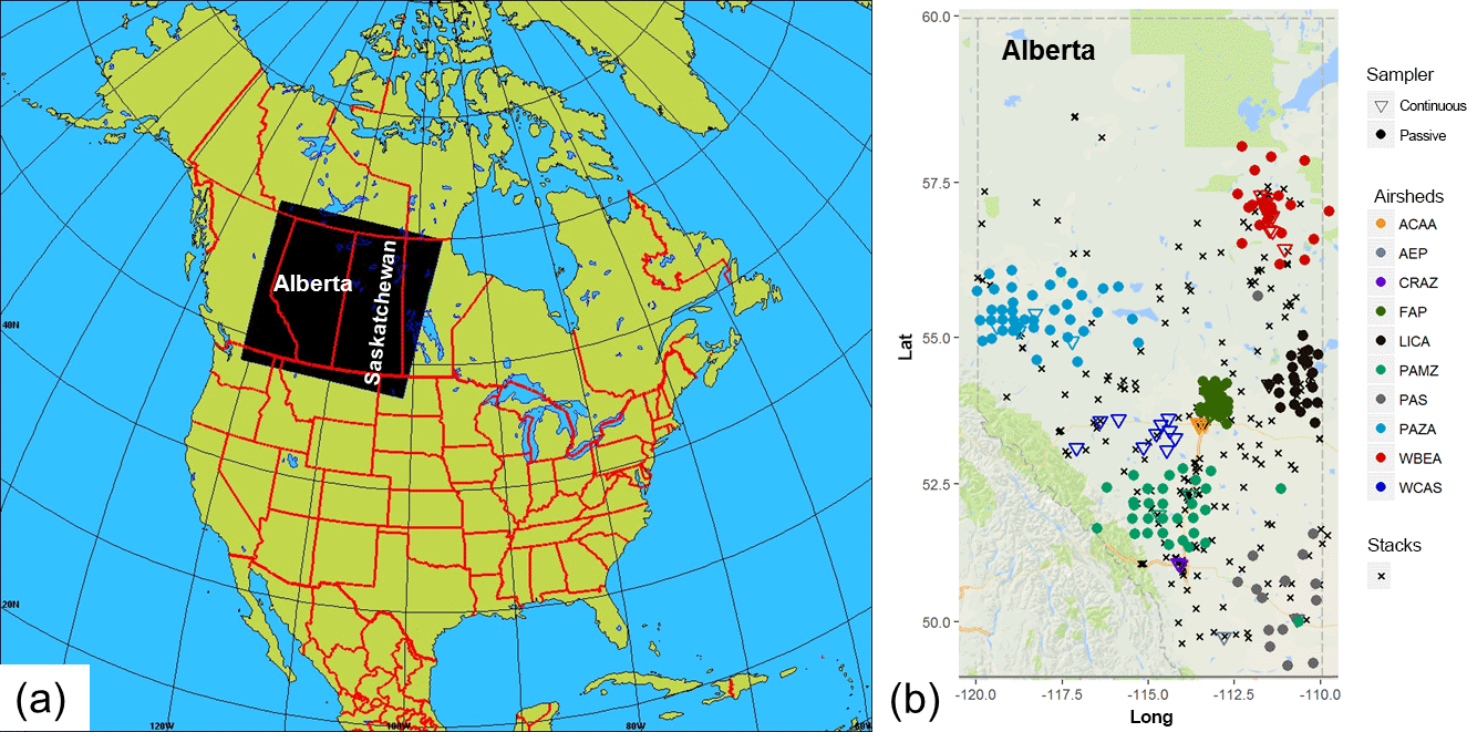
Figure 1Study area: (a) model domain covering the provinces of Alberta and Saskatchewan; (b) NO2 and SO2 continuous and passive monitors located at the different air quality monitoring networks (airsheds) and main NO2 and SO2 stacks in the province of Alberta. Stations are colour-coded according to airsheds and plotted with different polygons (circle for passive, inverted triangle for continuous): West Central Airshed Society (WCAS), Wood Buffalo Environmental Association (WBEA), Fort Air Partnership (FAP), Alberta Capital Airshed Alliance (ACAA), Calgary Regional Airshed Zone (CRAZ), Peace Airshed Zone Association (PAZA), Palliser Airshed Society (PAS), Parkland Airshed Management Zone (PAMZ), and Lakeland Industrial Community Association (LICA).
2.1 Study area
Alberta, one of the western provinces of Canada (Fig. 1), is the largest producer of conventional crude oil, synthetic crude and natural gas and gas products in Canada, and is home to one of the world's largest deposits of oil sand (a mixture of clay, sand, water, and bitumen; CAPP, 2018). The monitoring of atmospheric pollutants and the provision of public information on air quality in Alberta is carried out by non-profit organizations called “airsheds”; these organizations are responsible for air pollution monitoring in specified subregions of the province. Figure 1b shows the spatial distribution of these monitoring networks within the province, as well as the largest NO2 and SO2 stack emission sources (National Pollutant Release Inventory, NPRI, 2013). The relative proportion of emissions from different sources depends on the subregion. For example, in the Athabasca oil sands area (monitored by Wood Buffalo Environmental Association (WBEA) stations; red symbols, Fig. 1b), SO2 is mainly emitted from stacks (flue-gas desulfurization; “major point sources”) and NO2 is emitted from both stacks and off-road vehicle mine fleets (“area sources”). The 2013 total emissions for Alberta were approximately 681 kt for NOx (NO and NO2) and 311 kt for SO2, respectively.
2.2 Monitoring data
In this study we included observations from both passive and continuous instruments measuring NO2 and SO2 ambient concentrations, since these are the only two species in the available data that include observations from both measurement methodologies. The nine airsheds within Alberta are shown in Fig. 1b: West Central Airshed Society (WCAS), WBEA, Fort Air Partnership (FAP), Alberta Capital Airshed Alliance (ACAA), Calgary Regional Airshed Zone (CRAZ), Peace Airshed Zone Association (PAZA), Palliser Airshed Society (PAS), Parkland Airshed Management Zone (PAMZ), and Lakeland Industrial Community Association (LICA). Figure 1b colour codes the sampling site locations by airshed, with continuous station locations shown as circles and passive stations shown as inverted triangles.
Continuous sampling is typically carried out for regulatory compliance, where high temporal resolution is required in order to monitor short-term exceedances in highly variable concentrations of pollutants in ambient air. The continuous monitoring principles of ultraviolet pulsed fluorescence and chemiluminescence are used to detect and measure SO2 and NO2, respectively, in Alberta, and the maximum value for detection limits of the NO2 and SO2 continuous samplers is 1.0 ppbv (AEP, 2014, 2016). In contrast, passive sampling is carried out in order to determine monthly average ambient air concentrations of atmospheric compounds for determination of long-term trends, to assess of potential ecological exposure risks, and to understand the spatial distribution of the measured pollutant. The majority of the Alberta passive monitors for NO2 and SO2 were developed by Maxxam Analytics Inc. (Tang et al., 1997, 1999; Tang, 2001), with the exception of those employed by PAS (PAS, 2016). The detection limit for 30-day average NO2 and SO2 sampling periods with these samplers is 0.1 ppbv. We analyse here the data records from 39 continuous and 89 passive SO2 monitoring sites and 38 continuous and 88 passive NO2 monitoring sites within the province of Alberta.
Passive sampling techniques have several advantages such as ease of deployment, no power requirements, and low maintenance, and they have been used as an alternative to continuous monitors for monitoring temporal trends of air pollutants in remote areas (Krupa and Legge, 2000; Cox, 2003; Seethapathy et al., 2008; Bytnerowicz et al., 2010) and evaluation of air quality of large areas (Gerboles et al., 2006). Their disadvantages are low sensitivity, inability to resolve short-duration concentration peaks, and adverse effects of meteorological conditions on reported observations (Tang et al. 1997, 1999; Krupa and Legge, 2000; Tang, 2001; Kirby et al., 2001; Partyka et al., 2007; Fraczek et al., 2009; Salem et al., 2009; Zabiegala et al., 2010; Vardoulakis et al., 2011). Moreover, the passive monitors depend on monthly meteorological information, which are needed in order to calculate diffusion rates. This information is obtained from the nearest site with meteorological observations, as most Alberta passive sampling sites do not have collocated meteorological measurements. These constraining factors could influence the sampling and, therefore, the accuracy of the results, causing under- or overestimation of ambient gas concentrations in relation to continuous analysers (Krupa and Legge, 2000).
We first analyse the continuous data, reported as hourly values to Alberta and Environment and Parks (AEP) for the period from July 2013 through September 2014, in a manner similar to Solazzo and Galmarini (2015), by focusing on the variations associated with different timescales and the determination of relative redundancy levels for different continuous monitoring stations. The time period for this continuous-only analysis was chosen to overlap with the Environment and Climate Change Canada (ECCC) air quality model simulations (described further in Sect. 2.3). In a second analysis, continuous and passive observations encompassing the period from February 2009 to December 2015 were analysed together in an effort to cross-compare the different sampling methodologies. The intent of this second analysis was to determine the extent to which the two methodologies provide similar results, in addition to determining the relative redundancy levels for the passive monitoring stations. In the second analysis, the continuous data were time-averaged to a similar interval as the passive monitoring data (the passive data were typically available as monthly or bimonthly averages).
All data were extracted from AEP archives (http://airdata.alberta.ca/, last access: 20 February 2007) and were subjected to additional QA–QC procedures due to the requirement of cluster analysis methodologies that there are no gaps in the time series of observations. We followed the recommendations of Solazzo and Galmarini (2015): continuous station data should be rejected if their hourly data records for the analysis period have more than 10 % of the total data for the year missing or contain data gaps of more than 168 consecutive hours in duration. Missing data may indicate a calibration period or stations which came on- or offline during the analysis period. We also follow their recommendations that data gaps of 1 to 6 h duration are replaced by the linear interpolation between the nearest valid data on either side of the gap and, for data gaps of longer duration, the annual average of the non-gap data was used. No substantial difference was found between the resulting cluster analysis by filling the longer gaps with these long-term averages versus using the average of the same number of missing days both before and after the gap.
For the comparison between passive and continuous SO2 and NO2 observations, the hourly continuous station data records were subject to the same station rejection criteria and gap-filling procedures as described above. Passive samplers nominally record either 1-month or 2-month averages, depending on location. One-month data were averaged to bimonthly data in order to have a consistent time interval for the dataset. When one of the 2-monthly values was missing from the original data, the bimonthly average was treated as missing. Passive stations missing more than 25 % of the data over the 5-year period were rejected from the subsequent analysis. This rejection criterion was less stringent than that applied to continuous data but was necessary in order to achieve a balance between including monitoring sites with most complete data and attaining good spatial coverage. An inclusion criterion of less than 10 % for missing passive data would have reduced the number of SO2 passive sites in the analysis from 52 to 18 and NO2 passive sites from 39 to 18. The missing data were gap-filled using the averages for the given station for the remainder of the 5-year time period. The gap-filled continuous data for the 5-year period were averaged to the same bimonthly intervals as the passive data. The monitors included in this study are listed in Tables S1, S2, S3, and S4 in the Supplement for the continuous monitoring network analysis for NO2 and SO2 and passive monitoring network analysis for NO2 and SO2, respectively, in Supplement 1.
2.3 Modelling output
GEM-MACH (Moran et al., 2010; Makar et al., 2015a, b; Gong et al., 2015) is an online chemical transport model describing several air quality processes, including gas-phase (42 gases), aqueous-phase, and heterogeneous chemistry, and aerosol microphysical processes (nine particle species with a two-bin sectional representation in the configuration used here). GEM-MACH version 2 simulations were carried out for the period between August 2013 and July 2014, over a domain centred over North America with 10 km grid spacing. The resulting outputs were used as initial and boundary conditions for a nested set of simulations at 2.5 km resolution for a domain covering the provinces of Alberta and Saskatchewan (Fig. 1a). The model was driven by regulatory reported emissions and additional emissions data emissions developed for the model simulations of JOSM (see Zhang et al., 2018, for further details on the model emissions) to better simulate Athabasca oil sand surface mining and processing facilities.
GEM-MACH simulations have been previously evaluated for both NO2 and SO2 concentrations against monitoring network data and satellite observations and cross-compared to the output of other air quality models in Im et al. (2015), Wang et al. (2015), Makar et al. (2015a, b), and Moran et al. (2016). Further evaluation of GEM-MACH on the high-resolution domain used here can be found in Makar et al. (2018) and Akingunola et al. (2018).
We use the output from GEM-MACH in two ways: initially, hourly 2.5 km resolution model results were extracted at monitoring station locations, and then cluster analyses for the model and observation data were compared. This comparison was carried out in order to evaluate the extent to which the model could act as a proxy for the observations and provide any caveats on the observation analysis associated with time averaging, sampling errors, and accuracy of the observations. In our final analysis, we demonstrate the use of the model as a proxy for monitoring network design by treating every model grid cell as if it contained a monitoring station – the clustering analysis of this proxy “data” was then used to define subregions within the model domain which could be represented by a single station for different values of the clustering metric. We carried out this analysis on a 36-by-36 test cell subdomain centred on the Athabasca oil sands, but the methodology could be scaled to larger regions. The results of this final analysis are spatial maps at different levels of a given dissimilarity metric, which may then be used as an aid in determining the locations for observation stations in an optimized monitoring network.
3.1 Separating different timescales using KZ filtering
The KZ filter (Zurbenko, 1986) is a means of removing smaller timescales from a time series, based on an iterative moving average over a specific time window. The combination of the number of times the moving average is applied (m) and the duration of the averaging window (p) determines the timescales removed from the time series (KZm,p), following the energy characteristics of the filter. Filtering parameters m and p can be derived from the transfer function (see Eskridge et al., 1997, and Zurbenko, 1986, for details on the transfer function). The removal of high-frequency variations in the data allows different timescales to be isolated and analysed separately. The KZ filter belongs to the class of low-pass filters.
For our analysis, hourly continuous time series data were KZ-filtered to remove short timescale variations, resulting in three additional datasets, which have had filtered-out time variations with periods less than a day (KZ17,3), a week (KZ95,5), and a month (KZ523,3). The subsequent analysis may thus examine the effect of removing the signal of the different timescales on the relationships between the stations. The time series resulting from each level of filtering may then be cross-compared, using hierarchical clustering, described in the following section.
In previous work appearing in the literature (Solazzo and Galmarini, 2015), the KZ filter was used in a “band-pass” configuration. A “band pass” is the difference between two KZ filters, for two different frequencies, and was used in an attempt to isolate the energy between those two frequencies. However, Hogrefe et al. (2000, 2003) indicated that applying the difference in KZ filters for band-pass purposes does not separate the spectral components completely, with the energy spectrum overlapping between the neighbour components. Rather than each band defining an exclusive set of frequencies, some of the energy from one band could be detected by the neighbouring band. We carried out a detailed analysis of the band-pass configuration and confirmed the analysis of Hogrefe et al., further finding that this energy “leakage” between bands was sufficient that the frequency bands associated with the shorter timescales could not be distinguished from each other. However, the KZ filter in its original low-pass form was found to be able to separate the timescales in the test data accurately, simply by choosing m and p coefficients to ensure that all energy was removed below specific frequencies. Subsequent clustering was shown to distinguish the influence of the different timescales, given an appropriate choice of the filtering parameters m and p. Our detailed analysis of the KZ filter in low-pass and band-pass configurations is described in detail in Supplement 2. Note that the m and p values used in this study were chosen to give an equivalent impact as band-pass filters used in Solazzo and Galmarini (2015).
It should be noted that time filtering and time averaging do not provide the same information. In the case of low-pass time filtering, the higher-frequency variation above some frequency is removed from the time series, while in the case of averaging that information is added to the average.
3.2 Dissimilarity analysis using hierarchical clustering
“Dissimilarity analysis” encompasses a group of methodologies used to rank datasets based on the extent to which they are different (or dissimilar) from each other. Dissimilarity may thus be used to rank stations in terms of potential redundancy such that stations with low levels of dissimilarity may be similar enough to be redundant. One of the most commonly used methodologies for dissimilarity analysis is hierarchical clustering (Johnson and Wicherrn, 2007).
The first step for hierarchical clustering is to choose a metric to describe how dissimilar the time series are from each other. This metric is then calculated for all possible pairs of the time series comprising the dataset. This initial set of calculations results in a dissimilarity matrix, which may then be used to cluster the data, based on the level of dissimilarity. The pair of time series with the lowest level of dissimilarity is combined and forms the first cluster. The metric of dissimilarity is then recalculated between the first cluster and the remaining time series, followed by pairing time series and/or clusters with the lowest dissimilarity in the reduced matrix. The number of clusters, which was originally equal to the number of time series in the original dataset, is thus reduced at each stage of the hierarchical clustering process; the process will be completed when the two last clusters have joined.
In this work, we have used two dissimilarity metrics: (1) 1−R, where R is the Pearson linear correlation coefficient (Solazzo and Gamarini, 2015), and (2) the Euclidean distance (the latter is the square root of the sum of the squares of the differences between the two time series' members). The metric based on correlation assesses dissimilarities associated with the changes in concentration as a function of time, while the Euclidian distance metric assesses dissimilarities on the basis of magnitude, over the time period of the analysis. We included the Euclidean distance out of concern that 1−R alone would fail to assess the magnitude differences, which may be more important than correlation, for some monitoring network applications. An extreme example would be two perfectly correlated time series, one of which has average concentrations an order of magnitude lower than the first; such a comparison could result from two stations positioned at different distances in a line downwind from an emissions source. Using 1−R alone, one of these stations could be considered redundant despite the information inherent in the lower concentrations associated with increasing distance from the emissions source. For both metrics, the recalculation of the dissimilarity matrix is carried out here with the general averaging method (Næs et al., 2010), as it provides robust and accurate clustering, with a substantial reduction in the processing time required to generate clusters (Solazzo and Galmarini, 2015).
The level of dissimilarity at which individual station records, and then clusters of records, merge as each new cluster is called a “node”. The order in which station records merge, as well as the level of dissimilarity at which they merge, may be displayed in diagrams known as dendrograms. Dendrograms show the pattern of linkages between nodes as the analysis progressed, with the vertical axis representing the level of dissimilarity, vertical lines representing specific clusters, and horizontal lines joining the clusters representing the nodes where the clusters are linked. A dendrogram has the appearance of the roots of a tree, with the join between the lowest roots representing the node of the most similar time series and the trunk of the tree the point at which all data have been joined to clusters. Very similar stations are thus joined at the bottom of a dendrogram.
3.3 Assessing potential station redundancy
Hierarchical clustering as described above was used to assist in the evaluation of potential monitoring station redundancies (defined as the relative dissimilarity level at which a station joins a cluster), as one of many considerations that could influence decision-making on monitoring network design. Having carried out hierarchical clustering using station data, the values of the dissimilarity metric as stations join clusters may be used to define the extent of similarity between stations, as well as a relative ranking of stations based on these similarities. This provides a quick assessment of station record similarities and offers insight into how the records are related to each other with respect to their temporal variations (1−R) and magnitudes (Euclidean distance) throughout the time interval analysed. We would consider stations potentially redundant if stations highly correlate with each other (low 1−R levels) and if the Euclidean distance levels are low. To decide if stations are redundant or not, a level of 1−R and/or Euclidean distance should be set; all the stations clustering under the same cluster at that given level should be under consideration for being removed or moved.
An assessment of monitoring record redundancies must be made prudently, the metrics used should be carefully assessed, and the physical distance between the stations and emissions sources should be taken into consideration (see Sect. 7). The inherent limitations of the analysis should also be noted. These include the following:
-
The ranking of stations is relative and specific to a given chemical species, the corresponding set of station time series, and the parameters used for the hierarchical cluster analysis: metric of dissimilarity and the method to recalculate the dissimilarity matrix.
-
Stations excluded because of data incompleteness are not analysed and not evaluated for possible redundancies.
-
The methodology has been applied in the past using observations from existing monitoring stations in order to analyse the relative dissimilarity between those stations' data records. However, the methodology may also be applied to gridded model-generated concentration time series. The latter application provides information on possible new locations for monitoring stations for a given number of monitoring stations or dissimilarity level (this process is described in more detail in Sect. 6).
-
Other considerations may factor strongly into monitoring network decision redundancy: for example, the availability of roads and electrical power, regulatory requirements, and cost.
An important corollary to the first point above is that different methods used in hierarchical clustering may result in different relative rankings of station records. Station records which are highly similar when 1−R is used (this metric is unitless and zero (unity) for the most (least) similar time series or clusters) may be highly dissimilar when the Euclidean distance is used (the Euclidean distance will have units of the chemical species being analysed and will be zero for the most similar clusters, but the magnitude of the upper limit of dissimilarity will depend on the specific time series being clustered).
“Redundancy” with regards to the metrics examined here is thus relative to a given chemical species and dataset used for hierarchical clustering. Therefore, we do not propose specific thresholds of the two metrics for determining redundancy. We note also that the results of the analyses for two metrics may be combined – station data that are relatively similar under one metric may be examined for their degree of similarity under another metric. The metric levels at which these combinations are examined are themselves also qualitative, but station time series which are highly similar under multiple metrics are in turn a stronger indication of potential redundancy.
Despite the above limitations, the methodology is nevertheless highly useful. In the event of limited available resources for monitoring, an assessment of relative redundancy, through the use of more than one metric, may aid in decision-making. Aside from implying redundancy between two data records, a high level of similarity may also indicate that a station may provide more information to the network if placed elsewhere, as opposed to its current location. In the last part of the analysis (Sect. 6), we show how the methodology may be extended through the use of air quality model output to design dissimilarity-optimized air quality networks.
4.1 Spatial distribution of clusters
The dissimilarity analysis was applied to NO2 and SO2 observational time series data for all the stations complying with the QA–QC criteria described in Sect. 2. The dendrograms resulting from the analysis are provided in Supplement 1.

Figure 2Associativity analysis for observed NO2 hourly time series using 1−R as the metric to compute the dissimilarity matrix, assuming a dissimilarity level of (a) 0.75, (b) 0.65, and (c) 0.55. Stations are colour-coded by cluster, and airsheds are plotted with different polygons. The acronyms for the airsheds are as in Fig. 1.
The hierarchical clustering results for NO2 using 1−R as the dissimilarity metric are depicted in Fig. S1 in the Supplement. This NO2 dendrogram shows frequent clustering between stations within the same airshed (if represented by more than a single station) or airsheds that are in relatively close physical proximity, such as airsheds ACAA and FAP (see Fig. 1b). A horizontal line cutting across a dendrogram such as Fig. S1 may be used to define the station records that are part of a cluster at a given level of the dissimilarity metric, and these may be plotted spatially: Fig. 2 shows the spatial distribution of the clusters of NO2 continuous monitors at three levels of the 1−R dissimilarity metric: 0.75 (Fig. 2a), 0.65 (Fig. 2b), and 0.55 (Fig. 2c). The results show that stations tend to cluster over successively smaller areas as the level of dissimilarity decreases (the three clusters of Fig. 2a as dissimilarity decreases become 11 clusters by Fig. 2c). The clustering at high dissimilarity levels (aka low correlation coefficients) also allows anomalous groupings of stations. For example, cluster 1 in Fig. 2a includes both WBEA stations at the upper right of the panel, one WCAS and one PAMZ station, despite the latter two sampling air in other parts of the province and being subject to different sources. This tendency is reduced at lower levels of dissimilarity, where stations influenced by similar sources tend to cluster. For example, in Fig. 2c, cluster 8 includes all the stations in a highly urbanized area (Edmonton, capital city of the province) and cluster 11 is a station located at a relatively high elevation upwind of most emission sources. Overall, the methodology shows the ability to group together monitoring station locations which might be expected to be influenced by similar sources of emissions.
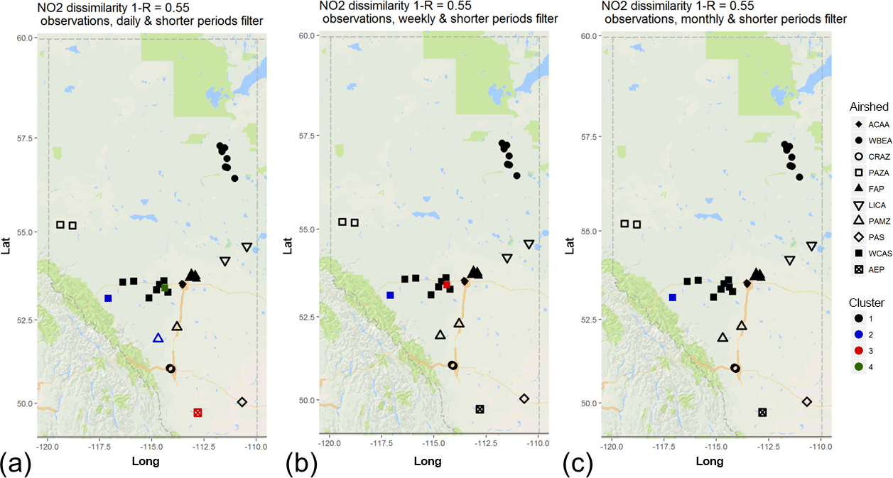
Figure 3Associativity analysis for observed NO2 filtered time series using 1−R as the metric to compute the dissimilarity matrix, assuming a dissimilarity level of 0.55: (a) daily, (b) weekly, and (c) monthly and short time periods. Stations are colour-coded according to cluster formation, and airsheds are plotted with different polygons. The acronyms for the airsheds are as in Fig. 1.
We next examine how the timescales inherent in the data may affect similarities. Figure 3 shows the clustering of stations which occurs at a 1−R dissimilarity level of 0.55 after timescales less than daily (Fig. 3a, dendrogram in Fig. S2), weekly (Fig. 3b, dendrogram in Fig. S3), and monthly (Fig. 3c, dendrogram in Fig. S4) are removed. Four clusters are shown on the first panel, three on the second, and two on the third. Comparing back to Fig. 2c with the original hourly data, this shows that much of the “signal” in 1−R contributing to the 11 clusters in Fig. 2c is contained within the shorter timescales of less than a day and are relatively similar at longer timescales. Moreover, correlation levels between stations increase as KZ filtering is applied and shorter time variability is removed. All of this evidence indicates that much of the variation in NO2 in the region takes place on relatively short timescales and is due to local sources. The analysis also indicates that some stations are more influenced by seasonality than others; e.g. the high altitude, largely upwind site of cluster 2 in Fig. 3c, remains separate from the other stations even when timescales of less than a month are removed from the analysis.
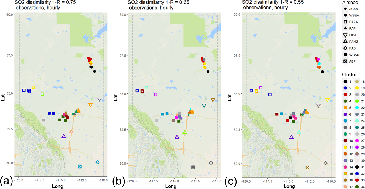
Figure 4Associativity analysis for observed SO2 hourly time series using 1−R as the metric to compute the dissimilarity matrix, assuming a dissimilarity level of (a) 0.75, (b) 0.65, and (c) 0.55. Stations are colour-coded by cluster, and airsheds are plotted with different polygons. The acronyms for the airsheds are as in Fig. 1.
The dissimilarity analysis for SO2 produced different results from that for NO2. Figure 4 shows the spatial distribution of the clusters of SO2 continuous monitors with the 1−R dissimilarity metric (the dendrogram resulting from the hierarchical clustering appears in Fig. S5) and can be compared to Fig. 2. For a given level of 1−R, there are more SO2 clusters than NO2 clusters. The observations of SO2, despite being largely collocated with the observations of NO2, are nevertheless more dissimilar than the observations of NO2. Even at higher levels of dissimilarity (compare Figs. 2a and 4a), there are more SO2 clusters, indicating a greater degree of local variability in the SO2 data, which drives correlation coefficients lower and dissimilarity levels for the 1−R metric higher. This greater degree of dissimilarity for SO2 is due to the nature of the SO2 emissions, i.e. almost exclusively from industrial “point” sources in the region under study, whereas NO2 concentrations are also influenced by more broadly geographically dispersed “area” sources of emissions including mobile on- and off-road vehicles. The dispersion of SO2 from the former source type is thus more dependent on very local meteorological conditions governing the rise of buoyant plumes from stacks than are the emissions from area sources. The direction and concentration of the rising and dispersing SO2 plumes are thus more highly variable in time compared to the area-source-dominated emissions of NO, which are chemically transformed rapidly to NO2. Concentrations from the same SO2 source may therefore not correlate to the same degree between different downwind stations as NO2. This contributes to the lesser degree of similarity between the SO2 station data even when monthly and shorter timescales are removed (the SO2 dendrograms with the removal of timescales less than daily, weekly, and monthly appear in Figs. S6, S7, and S8, respectively).
The Euclidean distance dendrograms for both NO2 (Fig. S9) and SO2 (Fig. S10) do not show the same distinctive clustering within airsheds as can be seen with the 1−R metric. This might be expected, as Euclidean distance between two time series may result from a single instance in which the hourly concentration records of the two stations differ substantially or several hours in which the concentration differences are smaller. Stations located sufficiently far apart that they monitor different sources of pollutants may thus have similar Euclidean distances if their average concentration magnitude is similar. The analysis also indicates that Euclidean distances become more similar in magnitude and that these magnitudes decrease, as increasingly larger timescales are filtered, across all of Alberta (Fig. S9 for NO2 and Fig. S10 for SO2). That is, concentration magnitudes recorded at the different stations approach each other as the shorter-duration time variations are removed. At these timescales, the magnitude of both species is driven by low concentration levels of long-term duration and larger spatial extent. This is particularly true for SO2 monitors that typically measure low concentration (background levels) interspersed with infrequent short-term high concentrations (surface fumigation events of buoyant plumes). However, within an airsheds affected by a common set of emissions sources, Euclidean distance will nevertheless be useful by identifying the presence of high-concentration gradients, as will be shown in the next section.
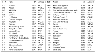
Table 1Hourly NO2 similarity ranking for the 1−R and Euclidean distance (EuD) metrics. Note that stations at the bottom of the two columns are the most similar (hence one measure of their level of redundancy) with respect to each metric of dissimilarity. Here we show only the first 10 and last 10 items of the ranking; the full ranking can be consulted in Table S5.
In summary, the methodology is able to identify groups of stations which are influenced by common emissions sources (e.g. stations which are influenced by oil sand emissions as opposed to stations located elsewhere) when the methodology is applied to hourly and, to some extent, daily time-filtered time series. Stations mainly influenced by seasonality are identified when the methodology is applied to weekly and monthly time-filtered data. The analysis groups stations according to their degree of similarity but does not provide the cause for that degree of similarity. The latter may only be achieved by examination of the data records and the use of local knowledge of sources and conditions. The level of information about the sources present in the study area will be greater when the results of both metrics are combined, and information about the sources may be inferred from the analysis; for example, stations could be classified as background or industrial impacted if seasonality or hourly data are shown to contain most of the signal.
4.2 Ranking of stations by dissimilarity
Previous work appearing in the literature (Solazzo and Gamarini, 2015) was motivated by the aims of evaluation and pre-screening of monitoring data for the purpose of the evaluation and development of regional-scale air pollution models. Their focus was on observations of ozone, which, in the troposphere, is a secondary pollutant resulting from gas-phase reactions and broader-scale chemistry and transport. They consequently focused on the different timescales associated with KZ filtering. Here, however, we have shown that for primary pollutants such as SO2 and “secondary” pollutants such as NO2, which are nevertheless very rapidly (on timescales of less than 5 min) produced from their primary precursors, much of the signal driving similarity resides at shorter timescales. Consequently, our ranking of continuous monitoring stations in this section is based solely on the original hourly observation data, as opposed to KZ-filtered observations.
The cluster analysis results for hourly time series were ranked from highest to lowest values of 1−R and Euclidean distance resulting from clustering of continuous monitoring station data. Stations clustering at high levels of 1−R and Euclidean distances are significantly different in time variation and concentration magnitudes, respectively. Conversely, stations at the bottom of the ranking are the most similar. The latter stations could be, therefore, considered potentially redundant. Our rankings are based on the dissimilarity level at which a given station joins another station as a new cluster or when a given station joins a pre-existing cluster. If the latter were to occur at a sufficiently low level of dissimilarity, either the new station or the pre-existing cluster might be considered potentially redundant. The uppermost and lowermost ranked stations for NO2 and SO2 are shown in Tables 1 and 2, respectively. The corresponding full ranking for the full list of stations is shown in Tables S5 and S6.
The tabulated values indicate clear differences between the two compounds. The stations measuring NO2 cluster with each other at substantially lower 1−R levels (that is, they correlate at substantially higher values of R) than do the stations measuring SO2. In one extreme case, the records of one SO2 station, Redwater Industrial, anti-correlate with the records of other stations, indicating that the SO2 time series at that location is substantially different from those of the remaining stations. However, the NO2 Euclidean distance metric cluster values tend to form at higher levels than their SO2 counterparts, with the exception of Redwater Industrial, indicating that despite their higher correlations, the NO2 stations may have larger differences in concentration magnitudes relative to SO2. We note that the Euclidean distance between SO2 station observations is, in many cases, relatively low (e.g. 24 ppbv for 8760 hourly values summed) and likely indicates stations which rarely record SO2 concentrations above background levels and hence have relatively “similar” Euclidean distances due to similarly low-concentration records for much of the recorded time series. Another interesting difference between the two atmospheric compounds is that the relative ranking by dissimilarity is closer to being the same for the two metrics for SO2 than for NO2.
Table 2Hourly SO2 similarity ranking. Note that stations at the bottom of the two columns are the most similar (hence one measure of their level of redundancy) with respect to each metric of dissimilarity. Here are only the first and last 10 items of the ranking; the full ranking can be consulted in Table S6.
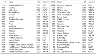
Two different dissimilarity metrics thus result in different relative rankings of the two chemical species, so the results must be interpreted with care. For example, the stations Fort McKay South and Fort McKay Bertha Ganter have the highest correlation for SO2 (R= 0.81) but their Euclidean distance is 177 ppbv, and a similar disparity between 1−R and Euclidean distance rankings for these stations may be seen in their values of the corresponding NO2 metrics (R= 0.84 and Euclidean distance of 411 ppbv). These stations are 4 km apart; the high correlation coefficients indicate that they may measure similar events, but the high Euclidean distances indicate that the magnitude of the events observed likely varies considerably despite the small separation distance. That is, substantial gradients in concentration may exist between the two stations at any given time. We note again here that low values of the dissimilarity metrics indicate a greater level of potential redundancy with respect to the rest of the stations – a high value of the Euclidean distance between two station records, or between a station record and a cluster, indicates that they are very dissimilar, and hence less potentially redundant. A second example is the pair of stations measuring NO2 with the lowest 1−R, Ross Creek and Fort Saskatchewan: these stations' data records are highly similar with respect to 1−R (that is, they are highly correlated), but the Euclidean distance between the two is 400 ppbv despite the stations being separated in distance by only 2.6 km. Again, the gradients in concentration between closely placed stations can be substantial. The intended purpose of the monitoring at such locations is key to assessing their level of potential redundancy. For example, if the aim of monitoring is to provide short-term exposure data for human health impacts, then these large Euclidean distances (despite the high correlations) indicate the presence of large gradients in concentration, and hence such station pairs should be considered less redundant. The combination of the metrics is thus shown to be important in network assessment – the addition of the Eulerian distance metric provides a broader context for station ranking than the use of 1−R alone.
Solazzo and Galmarini (2015) noted that clustering analysis can be used to determine the extent to which the different monitoring methodologies are comparable. Thus if different methodologies do not provide equivalent data, the clusters generated will be split according to methodology rather than being associated with local chemical and meteorological conditions. The combination of monitoring methodologies here thus has two purposes – to assess the relative dissimilarities between station records and to verify that both passive and continuous monitors provide similar data.
The hierarchical clustering methodology was applied to the 5-year bimonthly averaged time series sampled by continuous and passive monitors (we leave out the a priori KZ filtering step as the data in this case are already long-term averages). The dendrograms resulting from the clustering analysis are shown in Fig. S11 for NO2 and Fig. S12 for SO2. The spatial distributions for the station clusters for the 1−R dissimilarity metric will be the focus here.
The spatial distributions of the NO2 clusters at dissimilarity levels of 0.55 and 0.5 are shown in Fig. 5a and b, respectively, with the locations of continuous monitors plotted as inverted triangles and passive monitors as circles. At correlation level R= 0.45 (Fig. 5a) there is a clear distinction between passive and continuous monitors; all the continuous monitors belong to cluster 1, independent of their spatial location. A large number of the passive monitors also fall within this cluster; however, when a slight increase in correlation is applied (Fig. 5, R= 0.5), the clustering pattern changes significantly – most of the continuous monitors remain within the same cluster, but the passive monitors form separate clusters. Two WCAS continuous monitors separate and form a separate cluster at dissimilarity level 0.5 (Fig. 5b). Figure 5 also shows several cases of collocated continuous and passive monitors which do not fall within the same cluster for correlation levels of 0.5 or higher. The analysis shows that as higher levels of correlation are required, the continuous and passive monitors for NO2 do not cluster together despite close physical proximity or even collocation. Some of the passive monitor clusters at R= 0.5 (Fig. 5b) appear anomalous; for example, cluster 3 (red) includes stations in LICA and WBEA, despite these airsheds being separated by a distance of several hundred kilometres. As the level of dissimilarity is decreased from 0.55 to 0.5, the biggest difference in clustering patters is seen for WBEA monitors (in the upper right of the panels of Fig. 5) as passive and continuous monitors located closer to the oil sands facilities fall within cluster 1, while some of the passive monitors farther from the oil sands facilities fall within cluster 3. For levels of correlation above 0.5, the clustering between stations monitoring similar source areas is rare, independent of the airsheds (see dendrogram in Fig. S8).
Figure 6 depicts the clustering results for SO2 based on the 1−R metric for dissimilarity levels 0.75 (Fig. 8a) and 0.65 (Fig. 8b). Higher dissimilarity levels were used as examples for the generation of spatial distributions than for NO2 in this figure. The highly variable nature of the SO2 concentrations, as a result of their origin in stack emissions, results in a greater degree of variability inherent in the collected data, as described earlier (at lower dissimilarity levels, the number of clusters increases markedly). Comparing Figs. S9 and 6, most of WBEA passive and continuous monitors in the north-east of the region form a common cluster at R= 0.25 (Fig. 6a, cluster 11, red). However, at this low correlation level, a common cluster connects sites in LICA, FAP, WBEA, and PAZA airsheds, despite these sites being widely separated in space and influenced by different local sources of SO2 (cluster 12, green, Fig. 6a). At the slightly higher correlation level of R= 0.35 (Fig. 6b), the clustering across airsheds has been reduced, though LICA and FAP still share a common cluster (number 4, light blue). Again, the most direct interpretation of the differences between the SO2 and NO2 results for the 1−R metric analysis, when passive and continuous monitors are clustered together, is that the data time series records for SO2 are more highly variable than for NO2. If 1−R similarity is used for assessing potential station redundancies, then there is a lesser overall degree of potential redundancy in the SO2 data due to its greater degree of variability. However, the cause of that variability should also be considered. For example, we note again that some of the collocated passive and continuous monitors for SO2 do not fall within the same cluster at lower 1−R values (these are shown as different colours in overlapping inverted triangles and circles in Fig. 6b). This indicates that at least some of the variability may reside in the measurement methodologies employed.
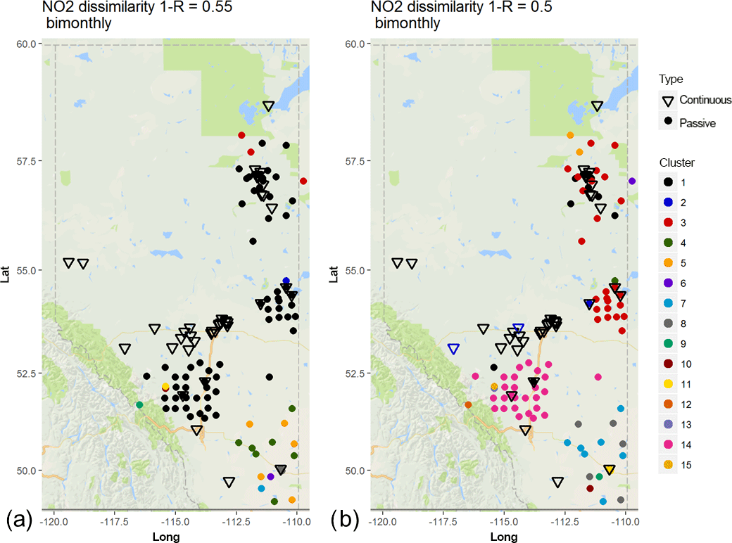
Figure 5Associativity analysis for passive and continuous bimonthly NO2 averages for 1−R = 0.55 (R= 0.3) Stations are colour-coded according to cluster formation, with continuous stations are marked as inverted triangles and passive stations as circles. The acronyms for the airsheds are as in Fig. 1.
In their analysis of European ozone monitoring networks, Solazzo and Galmarini (2015) found similar patterns between different European nations, noting that the differences are likely related to different sampling methodologies, instrument sensitivities, and data acquisition protocols not being harmonized between the countries. The same seems to be true for the Alberta passive and continuous monitoring stations, as the 1−R cluster analysis shows that the continuous stations are more similar to each other within and across airsheds than they are to the passive stations within the same airsheds, or located nearby. Collocated continuous and passive stations do not always show high levels of similarity, which would be expected had they reported the same concentrations. We analysed WBEA data alone using the 1−R metric (dendrogram in Fig. S13) and found that most of the continuous monitors formed a separate cluster from the passive monitors at relatively high levels of the 1−R metric, indicating that the two sources of data provide fundamentally different records. Collocated passive and continuous monitors also tended to have high levels of the Euclidean distance (not shown). Thus, at least some of the variability noted with these datasets seems to lie with the overall sampling methodology, and related confounding factors, discussed further in Sect. 7.
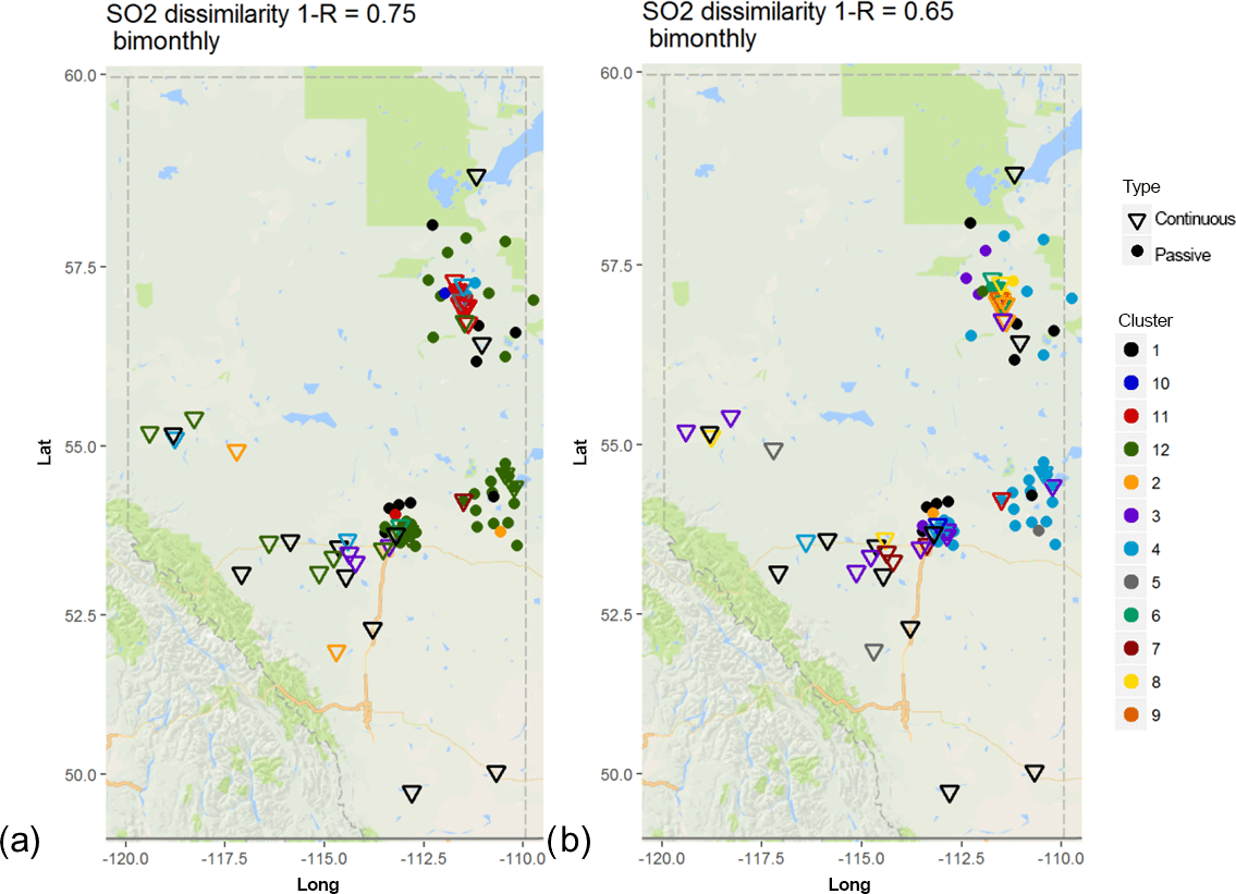
Figure 6Associativity analysis for passive and continuous bimonthly SO2 averages for 1−R = 0.7 (R= 0.3) Stations are colour-coded according to cluster formation, with continuous stations are marked as triangles and passive stations as circles. The acronyms for the airsheds are as in Fig. 1.
There have been several studies comparing passive and continuous analysers in Alberta (WBK, 2007; Hsu et al., 2010; Pippus, 2012; Bari et al., 2015). Bari et al. (2015), the study with the highest number of samples, cautioned that direct comparisons between NO2 and SO2 continuous and passive methods may be hampered by lower field accuracy in the passive methodology. Several studies show that passive samplers overestimate SO2 ambient concentrations and underestimate NO2 relative to continuous monitors. For example, the Bari et al. (2015) study showed that the median values for the absolute difference between the collocated passive and continuous monitors for NO2 is 1.5 and 0.2 ppbv for SO2. The same study assessed the relationship between passive and continuous measurements by regression analysis, concluding that the agreement between the different types of monitors is moderate, with the coefficient of determination being 0.42 and 0.40 for NO2 and SO2, respectively. We note that these previous comparisons were done for urban sites only; in this study we have carried out cluster analysis including passive and continuous monitoring data for rural, urban, and industrial sites outside of urban regions.
Air quality models such as GEM-MACH provide gridded time series concentrations of atmospheric pollutants and related chemicals at a common time interval, as a standard output. These are compared to observations in order to evaluate the model's performance (for traditional evaluations using the model output used herein, cf. Makar et al., 2018; Akingunola et al., 2018; Stroud et al., 2018). We introduce here for the first time the concept of the use of these time series of air quality model output, combined with hierarchical clustering analysis, as a surrogate for station data, for the purposes of monitoring network analysis and design. Two possible approaches can be taken. First, the model output at the model grid squares containing existing monitoring stations may be analysed in order to determine the extent to which the clustering analysis of model output mimics the clustering analysis of the corresponding observational data. Aside from presenting a new means by which the model output can be evaluated, this approach also can highlight possible causes for the observation data clustering results. The second approach is to use the gridded model output as a surrogate for a dense monitoring network (one “station” at every model grid square centre). The outcome of this second approach is a set of gridded maps – similar to the sparsely distributed observation location maps shown in the figures above, these show the clustering of potential stations. However, the cluster maps resulting from the use of the dense “network” of model grid squares define more precisely a set of regions, within each of which a single station may represent that larger region for the value of the dissimilarity metric chosen. We investigate this second approach from the standpoint of monitoring network design. Note that, in the work above, we have attempted to show how hierarchical clustering may be used to analyse existing monitoring networks; here we show how the same techniques, coupled with the output of a long-term simulation of an air quality model, can provide an optimized network design (where we here define “optimized” as “having a common level of dissimilarity for potential station locations, for the dissimilarity metrics chosen”). Equivalently, these optimized networks maximize the dissimilarity, and hence minimize the potential redundancy, in the location of monitoring network stations.

Figure 7Associativity analysis for modelled NO2 hourly time series using 1−R as the metric to compute the dissimilarity matrix, assuming a dissimilarity level of (a) 0.75, (b) 0.65, and (c) 0.55. Stations are colour-coded according to cluster formation, and airsheds are plotted with different polygons. The acronyms for the airsheds are as in Fig. 1.
Our first analysis using model output evaluates the extent to which the model is capable of creating similar clusters as the observations. Hourly model output for the 1-year simulation of GEM-MACH was extracted from those model grid squares containing the station locations, and the resulting time series data were submitted to the same hierarchical clustering methodology as described above. Figure 7 shows the spatial distribution for the cluster analysis at the same levels of 1−R, 0.75, 0.65, and 0.55, as was shown using observation data (compare to Sect. 4, Fig. 2). Each airshed is plotted with a different polygon, and colours indicate clusters. The corresponding dendrograms for these model results are shown in Fig. S14. Note that cluster colours and numbers differ between Figs. 2 and 7; stations fall within similar clusters in each figure. For SO2 dissimilarity level 1−R = 0.75 (Fig. 7a), the difference between the results for model and observations is not substantial; the clustering is identical aside from a single station in both WBEA and LICA, as well as AEP and PAS stations not forming separate clusters. The difference between observed and modelled NO2 clustering results is more notable as the level of dissimilarity decreases (Fig. 7b, c): the model tends to create a larger number of clusters than the observations at intermediate levels of dissimilarity (comparing Figs. 2b and 7b: 6 clusters versus 10 clusters; 2c and 7c: 11 clusters versus 13 clusters). The model results also tend to cluster within the same airsheds to a greater degree compared to the observations results. The model dendrograms tend to have clusters forming at higher levels of dissimilarity for some stations such as Steeper (Fig. S14 for Steeper is 1−R = 0.8, while Fig. S1 for Steeper's node is 1−R = 0.7). Some of these differences may be due to inaccuracies in the emissions data driving the model. For example, the major point source emissions data used in the simulations is based on regulatory reporting to the NPRI, wherein the regulatory requirement for reporting is an annual total. These annual totals must be temporally allocated using assumed temporal profiles for each source, and these month-of-year, day-of-week, and hour-of-day temporal profiles may not always match actual hourly emission levels at any given time. We show elsewhere (Akingunola et al., 2018) that hourly continuous emissions monitoring data used as model inputs may result in very different short-term concentration behaviour, with the corollary here that temporal allocation used here may influence the pattern of clusters. However, the model results at level of dissimilarity 0.65 tend to cluster more similarly with the observation results at level of dissimilarity at 0.55, indicating that the clustering analysis for the model results and observations show a similar spatial distribution, though the model shows overall higher correlation values than the observations.
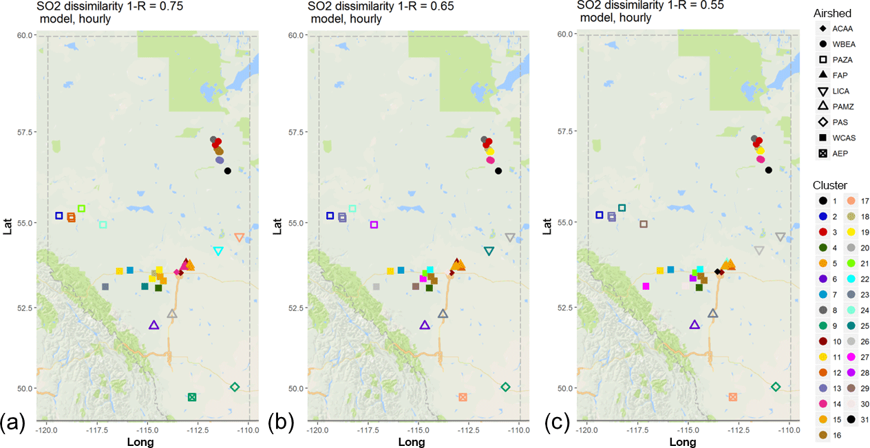
Figure 8Associativity analysis for modelled SO2 hourly time series using 1−R as the metric to compute the dissimilarity matrix, assuming a dissimilarity level of (a) 0.75, (b) 0.65, and (c) 0.55. Stations are colour-coded according to cluster formation, and airsheds are plotted with different polygons. The acronyms for the airsheds are as in Fig. 1.
The results for SO2 (dendrograms for the cluster analysis in Fig. S12, compare to Fig. S5) show the model results clustering similarly to the observations for PAMZ, ACCA, and WCAS stations. WBEA stations in the model results (Fig. S15, red station labels) are split into two clusters, while these stations are part of the same cluster in the observation-based analysis (Fig. S5). At 1−R level 0.75, both model and observation cluster analysis results (Fig. 8a, compare to Fig. 4a) already show many clusters composed of one or few stations, with the model showing slightly more clusters than the observations (21 clusters versus 25, respectively). As noted earlier, SO2 in this region is emitted mainly by point sources, and the use of annual emissions data with an assumed temporal allocation, along with the additional inherent difficulties in accurately predicting plume rise (Akingunola et al., 2018), makes the reproduction of the time record of SO2 by the model a challenge. Inaccuracies in both the emissions and the model meteorology may contribute to these differences.
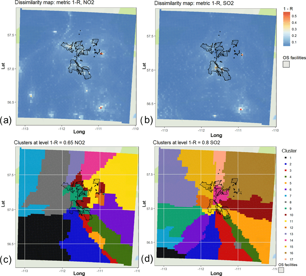
Figure 9Dissimilarity maps based on 1−R metric for (a) NO2 and (c) SO2 modelled hourly output at each GEM-MACH grid cell. Associativity analysis maps for modelled NO2 and SO2 based on these gridded output time series, appear in panels (b) and (d), respectively. The latter maps were generated using a (1−R) dissimilarity level of (b) 0.65 and (d) 0.8. All maps show the areas enclosing the property boundaries of the main mining facilities operating in the Athabasca oil sands region (black contours enclosing transparent light grey shading).
We next show an example of how hierarchical clustering using gridded model output may be used to generate an optimized monitoring network. For this analysis, we focus on a specific subsection of the model grid; namely a 72 × 72 block of model grid squares centred on the Athabasca oil sands. Figure 9 depicts the resulting mapped 1−R cluster analysis in this area, when each model grid cell has been treated as a potential monitoring station location. Figure 9a and c show the values of 1−R for each grid cell at the point in the analysis where that grid square becomes part of a cluster for NO2 and for SO2, respectively. Those grid cells with high values of 1−R thus join clusters at much lower correlation levels than those which have joined clusters at low values of 1−R. As a result, the maps show the extent of dissimilarity for the grid cells; higher values show grid cells which are so unlike others that they remain separate from the clusters throughout much of the analysis. In contrast, Fig. 9c and d show the clusters which exist for a specific level of 1−R. These show how the methodology may be used to design a monitoring network for a given number of stations (i.e. one station within each of the coloured regions will be sufficient to represent that coloured region, to within the value of 1−R used to generate the clusters). Figure 9b and d show the spatial distribution of the clusters generated by dissimilarity levels of 0.65 for NO2 and 0.8 for SO2, respectively (these levels were chosen based on the analysis above, where the model was shown to provide reasonable results). All the panels in Fig. 9 have the areas where the oil and gas extraction sites and processing facilities are located as a visual aid; these areas are contoured in black.
The 1−R metric maps (Fig. 9a and c) have the highest values where main emissions sources are located – these identify the main open-pit mine facilities of the oil sands, within which may be found both area and stack emissions sources. These regions of high variability are thus where the influence of the emissions and the local meteorology on the dispersion of the emissions is the strongest. In the NO2 dissimilarity map “point” (stack), “line” (roads) and “area” sources (mines) can be distinguished; for SO2 the locations of the stacks for processing and flaring are identified. The spatial distribution of the clusters (each cluster is mapped with a different colour in Fig. 9b and d) shows the areas wherein a single measurement station, placed anywhere within a given coloured region, would represent that region to the given level of dissimilarity. Figure 9c thus shows that for NO2 and for a 1−R dissimilarity level of 0.65, 17 monitoring stations, each placed at any location within each of the 14 coloured regions, would constitute an optimized network for NO2. Similarly, Fig. 9d shows that 17 stations would be required to monitor SO2 with a common 1−R dissimilarity of 0.80, and the regions over which those stations could each be placed. The analysis thus identifies regions which are equivalent from the standpoint of the dissimilarity metric used.
We note that in some cases a single cluster can be discontinuous, split into more than one area. An example of this can be seen in Fig. 9c, where a cluster is split into two separate red coloured regions (cluster 3), whereas Fig. 9d does not show the same split. Local knowledge of the emissions sources, as well as analysing Fig. 9a and b, help explain these results. The dark yellow region (cluster 5) in Fig. 9c and the grey region (cluster 8) in Fig. 9d mark the location of a local emissions source, moderate in magnitude relative to the larger sources in the middle of the domain (oil sand facility boundaries marked in these figures). The clustering thus recognizes the local influence of this moderate source of emissions; however, at greater distances from this source, the impact of the larger sources dominates. The red areas (cluster 3) in Fig. 9c and the green area (cluster 4) in Fig. 9d show that the larger sources have both a local and long-range influence, which only locally can be overwhelmed by the moderate source for both SO2 and NO2. We note that we are using 1−R in this application of the methodology with deterministic model output, so the magnitude of the signal of the two chemicals is not being analysed – rather, its time variation is. To satisfy different monitoring objectives, stations are placed by both geographical and physical location, with physical location defined by the concept of spatial scale of representativeness, the area where actual pollutant concentrations are reasonably uniform. We note that each of these coloured subregions in which a single station could be placed has a relatively large geographic extent and, using this metric, do not describe the concentration gradient in the region but could be used as a first guess for areas of representativeness, potentially providing useful input for applications such as data assimilation of air quality and meteorological observations. Combining spatial distribution of the clusters for 1−R metric with the Euclidean distance will provide further information about the concentration gradients in the area of representativeness. Note that maps such as these could be overlaid with other geographic information (e.g. road networks, the local power grid) to further optimize and decide on potential station locations. The similarity maps, combined with these other factors, could be used to aid in the design of air pollution monitoring networks.
The cluster distribution maps show that the areas for potential station location depend on the pollutant – the SO2 map is influenced to a greater degree by the wind directions throughout the year than NO2, likely due to the emissions sources for the former pollutant being driven almost entirely by stack sources in this region. The wind-rose-like pattern around SO2 sources likely stems from plume fumigation events at different times of the year, leading to a high correlation of SO2 concentrations leading downwind from the sources. The NO2 cluster distribution is patchier, reflecting both the impact of the stacks (which account for about 40 % of the total NO emissions in the region) and the off-road mobile mine fleet (other “area” sources, which account for the bulk of the remainder of the NOx emissions). If potential multi-pollutant monitoring station locations are desired, overlapping the optimized maps for each pollutant, for a given number of stations, would be a further way of aiding the monitoring network design process.
We also note that other metrics could be used in order to capture other aspects of concentration spatial and temporal variability, such as concentration gradients, in addition to temporal correlation – here we have demonstrated a “proof of concept”, and other metrics will be analysed in future work.
Factors that can negatively impact the results of hierarchical clustering include data dispersion (large variance between cluster members), outliers, and non-uniform cluster densities (clusters which are non-compact and non-isolated, and thus not properly distinct from one another; cf. Mangiameli et al., 1996; Milligan, 1980). However, we find that the analysis itself may also be used to identify these conditions. We have shown in the results in Sects. 4 and 5 that the analysis has indeed identified stations that are outliers relative to the rest of the dataset – these stations separate from the other stations as single-member clusters at high levels of dissimilarity. In other words, the analysis identifies the records of those stations as being substantially different from all other station records, for the dissimilarity metric used. This was particularly noticeable in the bimonthly data analyses. The methodology also identified cases of data dispersion, for example, the analysis of combined bimonthly passive and continuous monitors showed cases where monitors in close proximity or even collocated did not cluster together. The methodology thus seems capable of isolating outlier records and data dispersion as well as recognizing cases of substantial differences between data collection methodologies. The latter was noted in the case of hourly ozone observations by Solazzo and Galmarini (2015).
The analysis of combined continuous and passive data has identified systematic differences between the two monitoring methodologies as a potential confounding factor on the station ranking of passive stations; the analysis identifies collocated stations with concentration differences and poorly matching concentration time variation, but cannot identify the causes for these differences. These issues should be the subject of follow-up work. Nevertheless, we note that both passive and continuous data may be subject to errors associated with the accuracy and precision of the sampling methodology.
We examined the potential errors associated with the reported detection limit of the monitoring methodology by using the GEM-MACH derived time series at station locations. Random noise was added to the original model time series results, with the maximum magnitude of the noise for each species taken from the detection limit range of each instrument (i.e. random noise in the range ±0.5 ppbv was added to the NO2 time series and ±1 ppbv was added to the SO2 time series). The NO2 cluster results for hourly time series using 1−R as the dissimilarity metric (Fig. S13, compare to Fig. 2) show no significant difference between the original and noise-added time series. However, this changed as timescales were removed from the original datasets by KZ filtering, especially once monthly and all shorter timescales were removed. Random noise was thus shown to be a potential confounding factor in 1−R hierarchical clustering analyses. However, for the corresponding NO2 Euclidean distance metric, both the hourly and monthly filtered data, with and without noise added, resulted in identical clustering (not shown). The SO2 results showed a larger variation between the clusters generated with the original time series and those containing additional random noise. The difference in clustering was particularly noticeable for the 1−R dendrograms, for both hourly and time-filtered data, and slightly less pronounced for Euclidean distances (not shown). The work described above suggests that much of the “signal” for primary emitted or quickly reacting secondary pollutants for correlation analysis resides in the shorter timescales (hourly to daily); the greater influence of random noise on the results of the time-filtered data implies that the latter are dominated by close-to-background concentrations, which are in turn similar in magnitude to the noise levels added here, and hence a greater influence is seen on clustering of the time-filtered data. For species such as SO2, which are dominated by short-duration high-concentration plumes, this effect may extend to the shorter timescales as well.
Besides the detection limit of the instrument, airsheds report the passive observations with a reporting limit of 0.1 ppbv; hence we also tested the accuracy of the instrument or the number of significant figures being reported, again using the model time series at station locations as a surrogate for observation data. The model results were filtered for three or zero significant figures below the decimal, and the resulting analyses were compared. As for the random error test, we found that for both NO2 and SO2 the dendrogram patterns changed, indicating that the use of fewer significant digits in data reporting will result in enough loss of information to change the interpretation of the data.
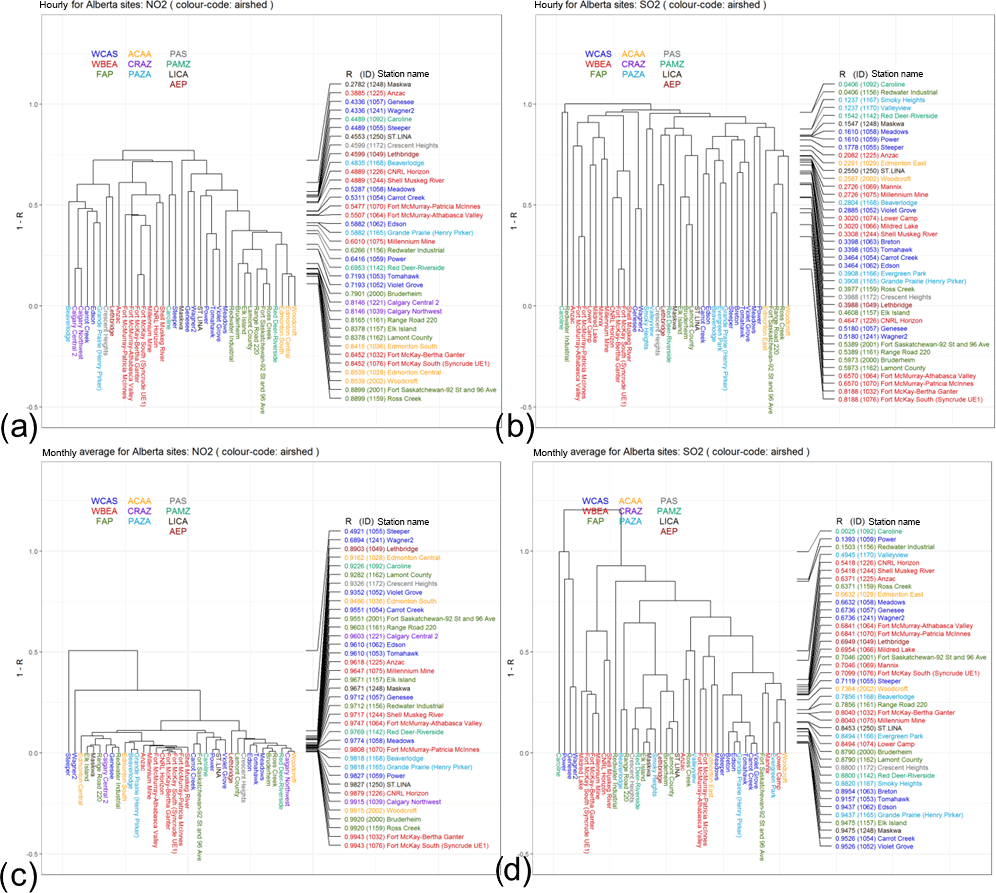
Figure 10Dendrogram analysis for NO2 and SO2 hourly (a and b, respectively) and monthly or shorter timescales time series (c and d, respectively) using 1−R as the metric to compute the dissimilarity matrix, for the airsheds described in Fig. 1. The dendrogram is colour-coded according to airsheds. Right side: stations ranked from low to high correlation level.
In the analysis described in Sect. 4, it was noted that as successively larger timescales are filtered from the data used for clustering, the magnitudes of the clustering metrics show an increasingly higher degree of similarity, with monitors clustering both within and across airsheds. However, the filtering of time series to remove successively larger timescales is not equivalent to averaging, in which shorter timescale information may be retained in the average. To specifically examine the effect of time averaging during data collection on clustering results, the clusters for the hourly data were compared to those from daily, weekly, and monthly averages (Fig. 10). With the original hourly data, specific airsheds were identified as unique clusters (as expected, for 1−R hierarchical clustering; stations located close to airshed-specific sources were identified as being more similar). However, with increasing averaging times, this airshed-specific clustering was gradually lost. Most of the information driving the ability of 1−R clustering to link local sources was thus shown to reside in the shorter timescales. Nevertheless, this information was lost as increasing averaging periods were applied (Fig. 10). A fundamental result of this analysis is that measurements that consist of long-term averages may lose the ability to identify the influence of local sources on the basis of time variation, i.e. they will correlate at an equal level with both adjacent monitoring stations and those that are located in distant regions. However, this information is retained in hourly records, and the latter may be used to identify unique source regions on the basis of correlation.
We note here that the results of analyses of this nature are dependent on the time series data used (including its duration). We have used a 5-year dataset to evaluate bimonthly observation data and a 1-year dataset to evaluate hourly data and deterministic model results. Longer time periods may be preferred in future applications to limit the potential impact of year-to-year variability. Nevertheless, if emissions change in the future, the analysis should be repeated in order to determine whether the pattern of clusters has changed in response to the changes in emissions. Similarly, while long time sets are desired from the standpoint of removing the potential impacts of annual variability in meteorological conditions, if changes in emissions happen frequently, it may argue for yearly rather than multi-year analyses.
A methodology for cross-comparing air quality monitoring networks was proposed here, expanding on the work of Solazzo and Galmarini (2015) by including the Euclidean distance as well as 1−R as dissimilarity metrics for hierarchical clustering and by making use of chemical reaction transport model output as a surrogate for observation station data. We adopted the KZ filter in its original low-pass configuration in order to improve the ability of the methodology to distinguish the impact of different timescales of variation on clustering. The Euclidean distance metric allowed cross-comparison of the stations in terms of the magnitude of the concentrations, whereas 1−R evaluated their temporal variation similarity. Both metrics can be used together or separately to evaluate the similarity of the stations and their potential redundancy. The relative level of potential redundancy for existing observation stations was ranked based on each dissimilarity metric, and we recommend evaluating monitoring station redundancy using both metrics where possible. Stations which form clusters at low values of both 1−R and Euclidean distance are the most redundant, while those with high values of either or both of these metrics are the least redundant. Absolute thresholds for redundancy cannot be generated since the relative rankings depend on the available observation data (number of stations and chemical species observed). In addition, other considerations, such as spatial proximity to sensitive receptors, the regulatory purpose of the station(s), and logistics (e.g. accessibility or power supply), may outweigh the recommendations based on similarity alone.
We have shown, through several analyses, that much of the observation signal which may be used to identify common sources of both primary pollutants and secondary products of fast reactions resides in shorter timescales (hourly to daily). When hourly data are available, the methodology is able to identify groups of stations that are influenced by common emissions sources (e.g. stations that are influenced by oil sand emissions as opposed to stations located elsewhere) as well as outliers or station records that are markedly different from all others in a given dataset. The former property is useful for identifying the influence range of specific emission sources. The latter property shows that the methodology is a useful tool for identifying station instrumentation that may be located such that they are subject to unique conditions (e.g. very nearby sources, anomalous long-term variation) or that have anomalous readings. However, for data consisting of longer-term averages, or observations in which the shorter timescales have been removed by filtering, at least some of the information which identifies the influence of common emissions sources is lost. Nonetheless, the methodology, when applied to time-filtered data, is able to single out stations mainly influenced by seasonality.
Clustering was shown to depend on the chemical species analysed, suggesting that optimization of networks using this methodology should be carried out on a “by species” basis rather than a “by station” basis. The two species examined here originate in different types of emissions sources in the region under study and consequently have different dissimilarity rankings for the corresponding stations.
We have corroborated the work of Solazzo and Galmarini (2015) for ozone in that the methodology is capable of identifying monitoring stations making use of different monitoring methodologies (via our 5-year analysis of passive and continuous SO2 and NO2 observations on a common bimonthly averaging interval). Passive and continuous monitors in the same airsheds did not always fall within common clusters (with several examples in which collocated monitors from the two technologies did not correlate). Some of these issues may be the result of averaging time, though data round-off and accuracy (random noise) were also shown to have a negative influence on the clustering results.
We have expanded the use of hierarchical clustering for air pollution to include its use with air quality model output. This presents a new avenue for monitoring network optimization and design in that each high-resolution air quality model grid square can be treated as a potential monitoring station location. Comparisons of the results of the clustering of model and observed time series at monitoring station locations showed clusters generated from model output tended to be more similar within airsheds than was the case for clusters generated from observations. However, the results are quite comparable, albeit at higher correlation levels for the model than the observations, and the match to observations depends on the chemical species. Tests in which gridded model output was treated as potential station locations resulted in the first dissimilarity-analysis-based maps of optimized air pollution monitoring networks. These showed that the methodology is capable of generating subregions within which a single station will represent that entire subregion, to a given level of a dissimilarity metric. Maps of this nature may be combined with other georeferenced data (e.g. road networks, power availability) to assist in monitoring network design.
While hierarchical clustering's pitfalls include data dispersion and outliers, we show here that the methodology is also able to identify differences in sampling methodologies and anomalous stations records. The analysis was shown to be particularly sensitive for monitors sampling air contaminants such as SO2 in areas of low background concentrations and sudden concentration peaks. For SO2, this is a result of the variation inherent in the type of sources that dominate SO2 emissions in our study region, i.e. large stack plumes. We also note that comparing observation-based cluster analysis with those of air quality model output at station locations might help identify possible deficiencies in the emission data used to drive air quality models. Given that short-term variation has been shown here to have a key impact on identifying common sources, the use of annual totals and assumed temporal profiles as the basis for emission inventory reporting should be avoided, and more time specific records, should be used where possible.
The continuous air quality observations are available from the publicly accessible database, http://airdata.alberta.ca/ (Airdata warehouse, 2018), and the passive observations can be made available upon request to Yayne Aklilu (AEP). The model results are available upon request to Paul A. Makar (ECCC). GEM-MACH, the atmospheric chemistry library for the GEM numerical atmospheric model (© 2007–2013, Air Quality Research Division and National Prediction Operations division, Environment and Climate Change Canada), is a free software which can be redistributed and/or modified under the terms of the GNU Lesser General Public License as published by the Free Software Foundation – either version 2.1 of the license or any later version. Much of the emissions data used in our model are available online: Executive Summary, Joint Oil Sands Monitoring Program Emissions Inventory report (https://www.canada.ca/en/environment-climate-change/services/science-technology/publications/joint-oil-sands-monitoring-emissions-report.html; Joint oil sands monitoring program emissions inventory report, 2018) and Joint Oil Sands Emissions Inventory Database (http://ec.gc.ca/data_donnees/SSB-OSM_Air/Air/Emissions_inventory_files/; Emissions inventory files, 2018). The cluster analysis code can be made available upon request to the main author (Joana Soares); the code is based on the work published by Cheng and Milligan (1996a, b, 1995).
The supplement related to this article is available online at: https://doi.org/10.5194/acp-18-6543-2018-supplement.
JS and PAM conceptualized and designed the study. JS applied the methodology, analysed the cluster analysis results and contributed to the writing of manuscript and modifications of same. PAM assisted in the analysis of the results, and contributed to the writing of the manuscript and modifications of same. YA provided the QC/QA AEP air quality monitoring data and contributed to the writing of the manuscript. AA provided the GEM-MACH simulations.
The authors declare that they have no conflict of interest.
This article is part of the special issue “Atmospheric emissions from oil sands development and their transport, transformation and deposition (ACP/AMT inter-journal SI)”. It is not associated with a conference.
This project was jointly supported by the Climate Change and Air Quality
Program of Environment and Climate Change Canada, Alberta Environment and
Parks, and the Joint Oil Sands Monitoring program. The figures in this
work were created using a combination of Environment Canada and Climate
Change software and the R open-source programming language (R Core Team,
2017).
Edited by: Randall Martin
Reviewed by: three anonymous referees
Airdata warehouse: Government of Alberta, available at: http://airdata.alberta.ca/, last access: 5 May 2018.
Akingunola, A., Makar, P. A., Zhang, J., Darlington, A., Li, S.-M., Gordon, M., Moran, M. D., and Zheng, Q.: A chemical transport model study of plume rise and particle size distribution for the Athabasca oil sands, Atmos. Chem. Phys. Discuss., https://doi.org/10.5194/acp-2018-155, in review, 2018.
Alberta Environment and Parks (AEP): Development of Performance Specifications for Continuous Ambient Air Monitoring Analyzers, Government of Alberta, AEP, Alberta, Canada, 2014.
Alberta Environment and Parks (AEP): Air Monitoring Directive Chapter 4: Monitoring Requirements and Equipment Technical Specifications, Government of Alberta, AEP, Air, No. 1–4, Alberta, Canada, 2016.
Bari, M. A., Curran, R. T. L., and Kindzierski, W. B.: Field performance evaluation of Maxxam passive samplers for regional monitoring of ambient SO2, NO2 and O3 concentrations in Alberta, Canada, Atmos. Environ., 114, 39–47, 2015.
Bauldauf, R. W., Wiener, R. W., and Heist, D. K.: Methodology for siting ambient air monitors at the neighborhood scalem, J. Air Waste Manage., 52, 1433–1452, https://doi.org/10.1080/10473289.2002.10470870, 2002.
Bytnerowicz, A., Fraczek, W., Schilling, S., and Alexander, D.: Spatial and Temporal Distribution of Ambient Nitric Acid and Ammonia in the Athabasca Oil Sands Region, Alberta, J. Limnol., 69, 11–21, 2010.
Canadian Association of Petroleum Producers (CAPP): The Facts on Canada's Oil Sands, available at: https://www.capp.ca/publications-and-statistics/publications/316441, last access: 24 April 2018.
Caselton, W. F. and Zidek, J. V.: Optimal monitoring network designs, Stat. Prob. Lett., 2, 223–227, https://doi.org/10.1016/0167-7152(84)90020-8, 1984.
Cheng, R. and Milligan, G. W.: Measuring the Influence of Individual Data Points in a Cluster Analysis, J. Classif., 13, 1432–1343, https://doi.org/10.1007/BF01246105, 1996a.
Cheng, R. and Milligan, G. W.: K-Means Clustering with Influence Detection, Educ. Psychol. Meas., 56, 833–838, https://doi.org/10.1177/0013164496056005010, 1996b.
Cheng, R. and Milligan, G. W.: Mapping Influence Regions in Hierarchical Clustering, Multivar. Behav. Res., 30, 547–576, https://doi.org/10.1207/s15327906mbr3004_5, 1995.
Cocheo, C., Sacco, P., Ballesta, P. P., Donato, E., Garcia, S., Gerboles, M., Gombert, D., McManus, B., Patier, R. F., Roth, C., de Saeger, E., and Wright, E.: Evaluation of the best compromise between the urban air quality monitoring resolution by diffusive sampling and resource requirements, J. Environ. Monitor., 10, 941–950, https://doi.org/10.1039/b806910g, 2008.
Cox, R. M.: The Use of Passive Sampling to Monitor Forest Exposure to O3, NO2 and SO2: a Review and Some Case Studies, Environ. Pollut., 126, 301–311, 2003.
Emissions inventory files: Government of Canada, available at: http://ec.gc.ca/data_donnees/SSB-OSM_Air/Air/Emissions_inventory_files/, last access: 5 May 2018.
Eskridge, R. E., Ku, J. Y., Rao, S. T., Porter, P. S., and Zurbenko, I. G.: Separating different scales of motion in time series of meteorological variables, B. Am. Meteorol. Soc., 78, 1473–1483, https://doi.org/10.1175/1520-0477(1997)078<1473:SDSOMI>2.0.CO;2, 1997.
European Environment Agency (EEA): Requirements on European Air Quality Monitoring Information, Topic report No 17/1996, available at: https://www.eea.europa.eu/publications/topic_report_1996_17 (last access: 18 September 2017), 1997.
Everitt, B. S., Landau, S., Leese, M., and Stahl, D.: Cluster Analysis, 5th Edn., Wiley Series in Probability and Statistics, 71–110, https://doi.org/10.1002/9780470977811.ch4, 2011.
Ferradás, E. G., Miñarro, M. D., Morales Terrés, I. M. M., and Martínez, F. J. M.: An approach for determining air pollution monitoring sites, Atmos. Environ., 44, 2640–2645, https://doi.org/10.1016/j.atmosenv.2010.03.044, 2010.
Fraczek, W., Bytnerowicz, A., and Legge, A.: Optimizing a Monitoring Network for Assessing Ambient Air Quality in the Athabasca Oil Sands Region of Alberta, Canada, Alpine Space Man & Environment, Global Change and Sustainable Development in Mountain Regions, 48, 127–142, 2009.
Gabusi, V. and Volta, M.: A methodology for seasonal photochemical model simulation assessment, J. Environ. Pollut., 24, 11–21, 2005.
Gerboles, M., Buzica, D., Amantini, L., Lagler, F., and Hafkenscheid, T.: Feasibility study of preparation and certification of reference materials for nitrogen dioxide and sulfur dioxide in diffusive samplers, J. Environ. Monitor., 8, 174–182, 2006.
Giri, D., Murthy, V. K., Adhikary, P. R., and Khanal, S. N.: Cluster analysis applied to atmospheric PM10 concentration data for determination of sources and spatial patterns in ambient air-quality of Kathmandu valley, Curr. Sci., 93, 684–688, 2007.
Gong, W., Makar, P. A., Zhang, J., Milbrandt, J., Gravel, S., Hayden, K. L., Macdonald, A. M., and Leaitch, W. R.: Modelling aerosol-cloud-meteorology interaction: A case study with a fully coupled air quality model (GEM-MACH), Atmos. Environ., 115, 695–715, https://doi.org/10.1016/j.atmosenv.2015.05.062, 2015.
Gramsch, E., Cereceda-Balic, F., Oyola, P., and Baer, D.: Examination of pollution trends in Santiago de Chile with cluster analysis of PM10 and ozone data, Atmos. Environ., 40, 5464–5475, 2006.
Hogrefe, C., Rao, S. T., Zurbenko, I. G., and Porter, P. S.: Interpreting information in time series of ozone observations and model predictions relevant to regulatory policies in the eastern United States, B. Am. Meteorol. Soc., 81, 2083–2106, 2000.
Hogrefe, C., Vempaty, S., Rao, S. T., and Porter, P. T.: A comparison of four techniques for separating different time scales in atmospheric variables, Atmos. Environ., 37, 313–325, https://doi.org/10.1016/S1352-2310(02)00897-X, 2003.
Hopke, P. K., Gladney, E. S., Gordon, G. E., Zoller, W. H., and Jones, A. G.: The use of multivariate analysis to identify sources of selected elements in the Boston urban aerosol, Atmos. Environ., 10, 1015–1025, 1976.
Hsu, Y.-M., Percy, K., and Hansen, M: Comparison of passive and continuous measurements of O3, SO2 and NO2 in the Athabasca Oil Sands Region, Proceedings of the 2010 (103rd) A&WMA Annual Conference, Air & Waste Management Association, Pittsburgh, PA, 2010.
Husain, T. and Khan, H. U.: Shannon's entropy concept in optimum air monitoring network design, Sci. Total Environ., 30, 181–190, https://doi.org/10.1016/0048-9697(83)90010-4, 1983.
Ibarra-Berastegi, G., Saienz, J., Ezcurra, A., Ganzeo, U., Elias, A., Barona, A., and Barinaga, A.:I dentification of redundant sensors in an air pollution network using cluster analysis and SOM, Air Pollution XVIII, WIT Trans. Ecol. Envir., 136, 359–366, 2010.
Ignaccolo, R., Ghigo, S., and Giovenali, E.: Analysis of air quality monitoring networks by functional clustering, Environmetrics, 19, 672–686, 2008.
Iizuka, A., Shirato, S., Mizukoshi, A., Noguchi, M., Yamasaki, A., and Yanangisawa, Y.: A cluster analysis of constant ambient air monitoring data from the Kanto region of Japan, Int. J. Env. Res. Pub. He., 11, 6844–6855, 2014.
Im, U., Bianconi, R., Solasso, E., Kioutsioukis, I., Badia, A., Balzasrini, A., Brunner, D., Chemel, C., Curci, G., Davis, L., van der Gon, H.D., Esteban, R. B., Flemming, J., Forkel, R., Giordano, L., Geurro, P. J., Hirtl, M., Hodsic, A., Honzka, L., Jorba, O., Knote, C., Kuenen, J. J. P., Makar, P. A., Manders-Groot, A., Pravano, G., Pouliot, G., San Jose, R., Savage, N., Schorder, W., Syrakov, D., Torian, A.,Werhan, J., Wolke, R., Yahya, K., Zabkar, R., Zhang, J., Zhang, Y., Hogrefe, C., and Galmarini, S.: Evaluation of operational online-coupled regional air quality models over Europe and North America in the context of AQMEII phase 2. Part II: Particulate Matter, Atmos. Environ., 115, 421–441, https://doi.org/10.1016/j.atmosenv.2014.08.072, 2015.
Ionescu, A., Candau, Y., Mayer, E., and Colda, I.: Analytical determination and classification of pollutant concentration fields using air pollution monitoring network data: Methodology and application in the Paris area, during episodes with peak nitrogen dioxide levels, Environ. Modell. Softw., 15, 565–573, https://doi.org/10.1016/S1364-8152(00)00042-6, 2000.
Jaimes, M., Roberto, M., Ortuño, C., Retama, A., Ramos R., and Paramo V. H.: Redundancy analysis for the Mexico City air monitoring network: the case of SO2, Proceedings of the Air and Waste Management Association's Annual Conference and Exhibition, available at: http://files.abstractsonline.com/CTRL/51/8/223/401/82C/47F/E9B/3CA/C0C/4C9/F43/1A/a1172_1.doc (last access: 19 November 2017), 2005.
Johnson R. A. and Wichern D. W.: Applied Multivariate Statistical Analysis, Pearson Prentice Hall, Pearson Education Inc. Upper Saddle River, NJ, USA, 2007.
Joint Oil Sand Monitoring (JOSM): Assessing The Scientific Integrity Of The Canada-Alberta Joint Oil Sands Monitoring (2012–2015) – Expert Panel Review, available at: http://aemera.org/wp-content/uploads/2016/02/JOSM-3-Yr-Review-Full-Report-Feb-19-2016.pdf (last access: 18 September 2017), 2016.
Joint oil sands monitoring program emissions inventory report: Government of Canada, available at: https://www.canada.ca/en/environment-climate-change/services/science-technology/publications/joint-oil-sands-monitoring-emissions-report.html, last access: 5 May 2018.
Kirby, C., Fox, M., Waterhouse, J., and Drye, T.: Influence of environmental parameters on the accuracy of nitrogen dioxide passive diffusion tubes for ambient measurement, J. Environ. Monitor., 3, 150–158, 2001.
Krupa, S. V. and Legge, A. H.: Passive Sampling of Ambient, Gaseous Air Pollutants: an Assessment from an Ecological Perspective, Environ. Pollut., 107, 31–45, 2000.
Lavecchia, C., Angelino, E., Bedogni, M., Bravetti, E., Gualdi, R., Lanzani, G., Musitelli, A., and Valentini, M.: The ozone patterns in the aerological basin of Milan (Italy), Environ. Softw., 11, 73–80, 1996.
Lindley, D. V.: On a measure of the information provided by an experiment, Ann. Math. Stat., 27, 986–1005, https://doi.org/10.1214/aoms/1177728069, 1956.
Lozano, A., Usero, J., Vanderlinden, E., Raez, J., Contreras, J., Navarrete, B., and Bakouri, H. E.: Design of air quality monitoring networks and its application to NO2 and O3 in Cordova, Spain, Microchem. J., 93, 211–219, https://doi.org/10.1016/j.microc.2009.07.007, 2009.
Lu, H.-C., Chang, C.-L., and Hsieh, J.-C.: Classification of PM10 distributions in Taiwan, Atmos. Environ., 40, 1452–1463, 2006.
Makar, P. A., Gong, W., Hogrefe, C., Zhang, Y., Curci, G., Zakbar, Milbrandt, J., Im, U., Galmarini, S., Balzarini, A., Baro, R., Bianconi, R., Cheung, P., Forkel, R., Gravel, S., Hirtl, M., Honzak, L., Hou, A., Jimenez-Guerrero, P., Langer, M., Moran, M. D., Pabla, B., Perez, J. L., Pirovano, G., San Jose, R., Tuccella, P., Werhahn, J., and Zhang, J.: Feedbacks between air pollution and weather, part 2: effects on chemistry, Atmos. Environ., 115, 499–526, https://doi.org/10.1016/j.atmosenv.2014.10.021, 2015a.
Makar, P. A., Gong, W., Milbrandt, J., Hogrefe, C., Zhang, Y., Curci, G., Zabkar, R., Im, U., Balzarini, A., Baro, R., Bianconi, R., Cheung, P., Forkel, R., Gravel, S., Hirtl, H., Honzak, L., Hou, A., Jimenz-Guerrero, P., Langer, M., Moran, M. D., Pabla, B., Perez, J. L., Pirovano, G., San Jose, R., Tuccella, P., Werhahn, J., Zhang, J., and Galmarini, S.: Feedbacks between air pollution and weather, part 1: Effects on weather, Atmos. Environ., 115, 442–469, 2015b.
Makar, P. A., Akingunola, A., Aherne, J., Cole, A. S., Aklilu, Y.-A., Zhang, J., Wong, I., Hayden, K., Li, S.-M., Kirk, J., Scott, K., Moran, M. D., Robichaud, A., Cathcart, H., Baratzedah, P., Pabla, B., Cheung, P., Zheng, Q., and Jeffries, D. S.: Estimates of Exceedances of Critical Loads for Acidifying Deposition in Alberta and Saskatchewan, Atmos. Chem. Phys. Discuss., https://doi.org/10.5194/acp-2017-1094, in review, 2018.
Mangiameli, P., Chen, S. K., and West, D.: A comparison of SOM neural network and hierarchical clustering methods, Eur. J. Oper. Res., 93, 402–417, 1996.
Mazzeo, N. and Venegas, L.: Design of an air-quality surveillance system for Buenos Aires City integrated by a NOx monitoring network and atmospheric dispersion models, Environ. Model. Assess., 13, 349–356, https://doi.org/10.1007/s10666-007-9101-y, 2008.
McGregor, G. R.: Identification of air quality affinity areas in Birmingham, UK, Appl. Geogr., 16, 109–122, 1996.
Milligan, G. W.: An examination of the effect of six types of error perturbation on fifteen clustering algorithms, Psychometrika, 45, 325–342, 1980.
Mofarrah, A. and Husain, T.: A Holistic Approach for optimal design of Air Quality Monitoring Network Expansion in an Urban Area, Atmos. Environ., 44, 432–440, https://doi.org/10.1016/j.atmosenv.2009.07.045, 2009.
Moran, M. D., Lupu, A., Zhang, J., Savic-Jovcic, V., and Gravel, S.: A comprehensive performance evaluation of the next generation of the Canadian operational regional air quality deterministic prediction system, Proc. 35th International Technical Meeting on Air Pollution Modelling and Its Application, 3–7 October, Chania, Crete, Greece, 6, 2016.
Moran, M. D., Menard, S., Talbot, D., Huang, P., Makar, P. A., Gong, W., Landry, H.,Gravel, S., Gong, S., Crevier, L.-P., Kallaur, A., and Sassi, M.: Particulate-matter forecasting with GEM-MACH15, a new Canadian air-quality forecast model, in: Air Pollution Modelling and its Application XX, edited by: Steyn, D. G. and Rao, S. T., Springer, Dordrecht, 2890–292, 2010.
Munn, R. E.: The design of air quality monitoring networks, Macmillan, London, England, 1981.
Næs, T., Brockhoff, P. B., and Tomic, O.: Statistics for Sensory and Consumer Science, 6th Edn., John Wiley & Sons, Ltd, Wiltshire, UK, ISBN: 9780470518212, 2010.
National Pollutant Release Inventory (NPRI): National Pollutant Release Inventory, available at: http://www.ec.gc.ca/inrp-npri/ (last access: 15 August 2017), 2013.
Omar, A. H., Won, J.-G., Winker, D. M., Yoon, S.-C., Dubovik, O., and McCormick, M. P.: Development of global aerosol models using cluster analysis of Aerosol Robotic Network (AERONET) measurements, J. Geophy. Res., 110, D10S14, https://doi.org/10.1029/2004JD004874, 2005.
Ortuño, C., Jaimes, M., Muñoz, R., Ramos, R., and Paramo, V. H.: Redundancy analysis for the Mexico City air monitoring network: the case of CO, Proceedings of the Air and Waste Management Association's Annual Conference and Exhibition, available at: http://files.abstractsonline.com/CTRL/2D/A/06E/7F9/022/434/F8D/F8C/2D3/E4B/F3E/66/a1177_1.doc (last access: 30 August 2017), 2005.
Palliser Airshed Society (PAS): A Year in the Palliser Airshed – 2006 Annual Report, Medicine Hat, Alberta, Canada, 2016.
Partyka, M., Zabiegala, B., Namiesnik, J., and Przyjazny, A.: Application of passive samplers in monitoring of organic constituents of air, Crit. Rev. Anal. Chem., 37, 51–78, 2007.
Pippus, G. J.: Assessment of Sources of Uncertainty in Passive Samplers of Ambient Air Quality: Evaluation Lakeland Industry and Community Association Airshed 2009–2011, MS thesis report, Royal Roads University, Victoria, BC, 2012.
Pires, J. C. M. Sousa, S. I. V., Pereira, M. C., Alvim-Ferraz, M. C. M., and Martins, F. G.: Management of air quality monitoring using principal component and cluster analysis – Part I: SO2 and PM10, Atmos. Environ., 42, 1249–1260, https://doi.org/10.1016/j.atmosenv.2007.10.044, 2008.
R Core Team: A language and environment for statistical computing, R Foundation for Statistical Computing, Vienna, Austria, available at: https://www.R-project.org/, last access: 18 November 2017.
Rhoades, B. J.: A methodology for minimizing and optimizing station location in a two-parametered monthly sampling network, Preprint 73–159, Pittsburgh, Air Pollut. Control Assoc., 1973.
Saksena, S., Joshi, V., and Patil, R. S.: Cluster analysis of Delhi's ambient air quality data, J. Environ. Monitor., 5, 491–499, 2003.
Salem, A., Soliman, A., and El-Haty, I.: Determination of nitrogen dioxide, sulfur dioxide, ozone, and ammonia in ambient air using the passive sampling method associated with ion chromatographic and potentiometric analysis, Air Qual. Atmos. Hlth., 2, 133–145, 2009.
Seethapathy, S., Górecki, T., and Li, X.: Passive Sampling in Environmental Analysis, J. Chromatogr. A, 1184, 234–253, 2008.
Solazzo, E. and Galmarini, S.: Comparing apples with apples: Using spatially distributed time series of monitoring data for model evaluation, Atmos. Environ., 112, 234–245, 2015.
Stroud, C. A., Makar, P. A., Zhang, J., Moran, M. D., Akingunola, A., Li, S.-M., Leithead, A., Hayden, K., and Siu, M.: Air Quality Predictions using Measurement-Derived Organic Gaseous and Particle Emissions in a Petrochemical-Dominated Region, Atmos. Chem. Phys. Discuss., https://doi.org/10.5194/acp-2018-93, in review, 2018.
Tang, H.: Introduction to Maxxam all-season passive sampling system and principles of proper use of passive samplers in the filed study, Proceedings of the International Symposium on Passive Sampling of Gaseous Air Pollutants in Ecological Effects Research, TheScientificWorld, 1, 463–474, 2001.
Tang, H., Brassard, B., Brassard, R, and Peake, E.: A new passive sampling system for monitoring SO2 in the atmosphere, FACT, 1, 307–315, 1997.
Tang, H., Lau, T., Brassard, B., and Cool, W.: A new all-season passive sampling system for monitoring NO2 in air, FACT 6, 338–345, 1999.
U.S. Environmental Protection Agency (US EPA): Ambient Air Monitoring Strategy for State, Local, and Tribal Air Agencies, available at: https://www3.epa.gov/ttnamti1/files/ambient/monitorstrat/AAMS for SLTs - FINAL Dec 2008.pdf (last access: 18 September 2017), 2008.
Vardoulakis, S., Solazzo, E., and Lumbreras, J.: Intra-urban and street scale variability of BTEX, NO2 and O3 in Birmingham, UK: Implications for exposure assessment, Atmos. Environ., 45, 5069–5078, https://doi.org/10.1016/j.atmosenv.2011.06.038, 2011.
Wang, K., Yahya, K., Zhang, Y., Hogrefe, C., Pouliot, G., Knote, C., Hodzic, A., San Jose, A., Perez, J.L., Jiménez-Guerrero, P., Baro, R., Makar, P., and Bennartz, R.: A multi-model assessment for the 2006 and 2010 simulations under the Air Quality Model Evaluation International Initiative (AQMEII) Phase 2 over North America: Part II. Evaluation of column variable predictions using satellite data, Atmos. Environ., 115, 587–603, https://doi.org/10.1109/GeoInformatics.2011.5980772, 2015.
WBK and Associates Inc (WBK): Field Precision and Accuracy of Maxxam Passive Samplers for NO2, O3, and SO2 Used in the Wabamun-Genesee Area Ambient Air Monitoring Program, St. Albert, AB, 13, 2007.
Zabiegala, B., Kot-Wasik, A., Urbanowicz, M., and Namiesnik, J.: Passive sampling as a tool for obtaining reliable analytical information in environmental quality monitoring, Anal. Bioanal. Chem., 396, 273–296, 2010.
Zhang, J., Moran, M. D., Zheng, Q., Makar, P. A., Baratzadeh, P., Marson, G., Liu, P., and Li, S.-M.: Emissions Preparation and Analysis for Multiscale Air Quality Modelling over the Athabasca Oil Sands Region of Alberta, Canada, Atmos. Chem. Phys. Discuss., https://doi.org/10.5194/acp-2017-1215, in review, 2018.
Zheng, J., Feng, X., Liu, P., Zhong, L., and Lai, S.: Site location optimization of regional air quality monitoring network in China: Methodology and case study, J. Environ. Monitor. 13, 3185–3195, https://doi.org/10.1039/c1em10560d, 2011.
Zhuang X. and Liu, R.: The optimization of regional air quality and monitoring network based on spatial analysis, Proceedings of the19th International Conference on Geoinformatics, 24–26 June 2011.
Zurbenko, I. G.: The Spectral Analysis of Time Series, North-Holland, Amsterdam, 236, 1986.
- Abstract
- Introduction
- Monitoring and air quality model data
- Associativity analysis for monitoring data based on dissimilarity
- Dissimilarity analysis for the continuous monitoring networks in Alberta
- Hierarchical clustering to cross-compare methodologies and technologies
- Model information as a potential surrogate for observations: optimized monitoring network design
- Potential factors impacting the analysis
- Conclusions
- Code and data availability
- Author contributions
- Competing interests
- Special issue statement
- Acknowledgements
- References
- Supplement