Ship-based MAX-DOAS measurements of tropospheric NO₂, SO₂, and HCHO distribution along the Yangtze River

In this paper, we present ship-based Multi-Axis Differential Optical Absorption Spectroscopy (MAX-DOAS) measurements of tropospheric trace gases' distribution along the Yangtze River during winter 2015. The measurements were performed along the Yangtze River between Shanghai and Wuhan, covering major industrial areas in eastern China. Tropospheric vertical column densities (VCDs) of nitrogen dioxide (NO₂), sulfur dioxide (SO₂), and formaldehyde (HCHO) were retrieved using the air mass factor calculated by the radiative transfer model. Enhanced tropospheric NO₂ and SO₂ VCDs were detected over downwind areas of industrial zones over the Yangtze River. In addition, spatial distributions of atmospheric pollutants are strongly affected by meteorological conditions; i.e., positive correlations were found between concentration of pollutants and wind speed over these areas, indicating strong influence of transportation of pollutants from high-emission upwind areas along the Yangtze River. Comparison of tropospheric NO₂ VCDs between ship-based MAX-DOAS and Ozone Monitoring Instrument (OMI) satellite observations shows good agreement with each other, with a Pearson correlation coefficient (R) of 0.82. In this study, the NO₂ ∕ SO₂ ratio was used to estimate the relative contributions of industrial sources and vehicle emissions to ambient NO₂ levels. Analysis results of the NO₂ ∕ SO₂ ratio show a higher contribution of industrial NO₂ emissions in Jiangsu Province, while NO₂ levels in Jiangxi and Hubei provinces are mainly related to vehicle emissions. These results indicate that different pollution control strategies should be applied in different provinces. In addition, multiple linear regression analysis of ambient carbon monoxide (CO) and odd oxygen (O_x) indicated that the primary emission and secondary formation of HCHO contribute 54.4 ± 3.7 % and 39.3 ± 4.3 % to the ambient HCHO, respectively. The largest contribution from primary emissions in winter suggested that photochemically induced secondary formation of HCHO is reduced due to lower solar irradiance in winter. Our findings provide an improved understanding of major pollution sources along the eastern part of the Yangtze River which are useful for designing specific air pollution control policies.

1 Introduction

Nitrogen dioxide (NO₂), sulfur dioxide (SO₂), and formaldehyde (HCHO) are important atmospheric constituents playing important roles in tropospheric chemistry. Nitrogen oxides (NO_x), defined as the sum of nitric oxide (NO) and NO₂, are one of the major pollutants in the troposphere, playing a key role in both tropospheric and stratospheric chemistry. It takes part in the catalytic formation of tropospheric ozone (O₃), while being a catalyst for the destruction of stratospheric O₃ (Crutzen, 1970). Major sources of NO_x are high-temperature combustions (e.g., fossil fuel burning and biomass burning) and natural processes (e.g., soil microbial activity and lightning events; Lee et al., 1997). NO₂ in high concentration is harmful to human health, especially for immune and respiratory systems. In addition, NO₂ can lead to the formation of nitrate aerosols, which is an important component of fine suspended particles in the urban environment. Sulfur dioxide (SO₂) is the most abundant anthropogenic sulfur-containing air pollutant. In urban areas, SO₂ is produced mainly through the combustion of sulfur-containing fossil fuels for power generation and domestic heating, which accounts for more than 75 % of the total SO₂ emissions (Chin et al., 2000). Atmospheric SO₂ causes similar environmental problems to NO₂, such as acidification of the natural aqua system and formation of secondary aerosols, and causes negative impacts on human health (Chiang et al., 2016). The atmospheric lifetimes of both NO₂ and SO₂ are relatively short, ranging from a few hours up to a few days (Krotkov et al., 2016), therefore, their spatial distributions are highly influenced by the emission sources.

Formaldehyde (HCHO) is one of most abundant volatile organic compounds (VOCs) in the atmosphere, playing an important role in air quality and atmospheric photochemistry. Incomplete combustion processes including industrial emissions and vehicle exhaust have been identified as major HCHO sources in the urban atmosphere (Garcia et al., 2006). Formaldehyde can also be produced from the atmospheric photochemical oxidation of methane (CH₄) and non-methane hydrocarbons (NMHCs) (Miller et al., 2008). In the polluted regions, terminal alkenes such as isoprene, ethene, and propene are the most important HCHO precursors (Goldan et al., 2000). The major sinks of HCHO are photolysis, reaction with OH radical, and wet deposition in the atmosphere (Lei et al., 2009). The atmospheric lifetime of HCHO under sunlight is typically very short (2–4 h), indicating that the daytime ambient HCHO is mostly produced locally (Arlander et al., 1995).

Multi-Axis Differential Optical Absorption Spectroscopy (MAX-DOAS) is a passive remote sensing technique providing indispensable information of atmospheric aerosols and trace gases (Platt and Stutz, 2008). Information of tropospheric trace gases is obtained from the molecular absorption in the ultraviolet (UV) and visible (VIS) wavelength bands by applying the differential optical absorption spectroscopy (DOAS) method to the observations of scattered sun light spectra in several different viewing directions. This method has been widely used for atmospheric NO₂, SO₂, and HCHO in the past decades (Lee et al., 1997; Heckel et al., 2005; Wang et al., 2014; Hendrick et al., 2014; Chan et al., 2015). MAX-DOAS observations are not only limited to ground-based applications, but also can be performed on different mobile platforms like cars (Johansson et al., 2009; Ibrahim et al., 2010; Shaiganfar et al., 2011), aircraft (Baidar et al., 2013; Dix et al., 2016), or ships (Sinreich et al., 2010; Peters et al., 2012; Takashima et al., 2012; Schreier et al., 2015). In this study, ship-based MAX-DOAS measurements of NO₂, SO₂, and HCHO were performed along the Yangtze River. Previous ship-based MAX-DOAS measurements were mainly focused on remote and coastal marine environments to obtain boundary layer background concentrations of trace gases, such as in the Indian Ocean and the Pacific Ocean. In this study, we performed ship-based MAX-DOAS observations along the Yangtze River, the busiest navigable inland waterway in the world, to obtain insight spatial distribution information of trace gases in eastern China.

The Yangtze River Delta (YRD) is one of the most populated regions in China. Due to rapid industrialization and urbanization in the past 2 decades, the YRD is facing a series of air pollution problems. As emission sources are not well characterized and the atmospheric processes are rather complex, it is important to measure the spatial distribution of atmospheric pollutants, i.e., NO₂, SO₂, and HCHO, in the YRD for the investigation of emission sources and atmospheric processes. This provides scientific support for designing prevention and control measures of air pollution. In this study, spatial distribution of tropospheric NO₂, SO₂, and HCHO was retrieved from ship-based MAX-DOAS observations along the Yangtze River between Shanghai and Wuhan. The experiment aims to provide improved understanding of emission sources and atmospheric processes over eastern China, which is potentially useful for the formulation of strategic air pollution control and identification of the effectiveness of air pollution control policies.

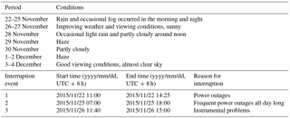
Table 1 Weather and viewing conditions during the Yangtze River campaign from 22 November to 4 December 2015. Interruption of the ship-based MAX-DOAS is also listed.

In this paper, we present ship-based Multi-Axis Differential Optical Absorption Spectroscopy (MAX-DOAS) measurements of tropospheric trace gases' distribution along the Yangtze River during winter 2015. The measurements were performed along the Yangtze River between Shanghai and Wuhan, covering the major industrial areas in eastern China. Details of the experimental setup, spectral analysis, and trace gases' retrieval of the ship-based MAX-DOAS measurement is presented in Sect. 2. The comparison with the Ozone Monitoring Instrument (OMI) NO₂ and the contribution of major emission sources to NO₂ levels along the Yangtze River as well as the contribution of primary and secondary sources of HCHO are shown in Sect. 3.

Table 2 Summary of the DOAS retrieval settings used for the NO₂, SO₂, and HCHO slant column densities' retrieval.

^* Solar I₀ correction; Aliwell et al. (2002).

2 Methodology

2.1 The Yangtze River measurement campaign

The Yangtze River campaign took place in winter 2015 along the Yangtze River over eastern China within the framework of the “Regional Transport and Transformation of Air Pollution in Eastern China”. The aims of the Yangtze River campaign are to provide better understanding of the transportation and transformation of atmospheric pollution and to identify the potential impacts on air quality and climate.

Ship-based measurement campaign was carried out along the eastern part of the Yangtze River between Shanghai and Wuhan. The campaign includes a departing journey (from Shanghai to Wuhan) and a returning journey (from Wuhan to Shanghai). The measurement campaign started on 21 November 2015 at 19:30 LT (local time) from Shanghai (31.36^∘ N, 121.62^∘ E), a major industrial and commercial hub of eastern China, and arrived in Wuhan (30.62^∘ N, 114.32^∘ E) on 29 November 2015 at 15:42 LT. The measurement ship then directly sailed back and finally arrived in Shanghai on 4 December 2015 at 20:30 LT. The journey covered most of the major industrial areas in eastern China including several population-dense metropolitan cities, such as Nanjing, Wuhu, and Jiujiang. Detail of the cruise track is shown in Fig. 1.

Figure 1 The ship tracks of (a) the departing journey (from Shanghai to Wuhan) and (b) the returning journey (from Wuhan to Shanghai). The sections of the cruise track highlighted in orange indicate the period of MAX-DOAS observations. The green dots represent the major power plants along the Yangtze River.

The ship-based MAX-DOAS instrument was part of the air quality monitoring framework of the Yangtze River measurement campaign. The instrument was installed at the beginning of the measurement campaign and started to provide atmospheric observations on 22 November 2015. A summary of the meteorological conditions during the Yangtze River campaign is shown in Table 1.

2.2 MAX-DOAS measurements

2.2.1 Experimental setup

Ship-based MAX-DOAS measurements were performed during the Yangtze River campaign. The ship-based MAX-DOAS instrument was developed at the Anhui Institute of Optics and Fine Mechanics (AIOFM), Chinese Academy of Sciences (CAS), which consists of a telescope, a spectrometer, and a computer acting as a controlling and data acquisition unit. Viewing directions of the telescope are controlled by a stepping motor, and scattered sunlight collected by the telescope is redirected to the spectrometer for spectral analysis through an optical fiber bundle. The field of view of the telescope is estimated to be less than 1^∘. An imaging spectrometer (Princeton instrument), equipped with a charge-coupled device (CCD) detector (512 × 2048 pixels) is used to measure spectra in the UV wavelength range from 303 to 370 nm with a spectral resolution of 0.35 nm full width half maximum (FWHM). Spectral data recorded by the imaging spectrometer were averaged along the first dimension of the CCD in order to get a better signal-to-noise ratio. During the measurement campaign, the viewing azimuth angle of the telescope was adjusted to 90^∘ (right) relative to the heading direction of the ship (see Fig. S1 in the Supplement). A full measurement sequence includes elevation angles (α) of 30 and 90^∘ (zenith). The exposure time of each measurement is set to 100 ms.

2.2.2 Data processing and filtering

Although the instrument was positioned in front of the exhaust stack (see Fig. S1 in the Supplement), the MAX-DOAS measurements could still be influenced by the exhaust from the ship. Therefore, measurement data contaminated by the ship exhaust were filtered out in our analysis. Individual measurements taken under unfavorable wind directions (relative wind directions between 150 and 270^∘ with respect to the heading of the ship) were discarded in the following analysis. Due to the stronger absorptions of stratospheric species and low signal to noise ratio at large solar zenith angles (SZAs), only measurements with a solar zenith angle smaller than 75^∘ were taken into account for the DSCDs' retrieval. With these filtering criteria (unfavorable wind directions and SZAs), 5.4 and 15.8 % of all data were rejected before DSCDs' retrieval, respectively.

As the viewing elevation angles of the measurements were relatively high (30 and 90^∘), they are therefore insensitive to the instability or the movement of the ship. In addition, since the exposure time of a measurement is rather short (100 ms), the change of measurement elevation and azimuth angle during one measurement is negligible.

2.2.3 DOAS retrieval

Differential slant column densities (DSCDs) of trace gases are derived from the measurement spectra by applying the differential optical absorption spectroscopy (DOAS) technique (Platt and Stutz, 2008). In this study, MAX-DOAS spectra are analyzed using the QDOAS spectral fitting software suite developed by BIRA-IASB (http://uv-vis.aeronomie.be/software/QDOAS/). The wavelength calibration was performed by using a high-resolution solar reference spectrum (Chance and Kurucz, 2010). The dark current (DC) spectrum was taken with an exposure time of 3000 ms and with 20 scans, while the electronic offset spectrum (OFFSET) was taken with an exposure time of 3 ms and with 20 000 scans. The dark current and offset spectra were used to correct measurement spectra prior to the spectra analysis. Several trace gas absorption cross sections (Vandaele et al., 1998, 2009; Meller and Moortgat, 2000; Serdyuchenko et al., 2014; Thalman and Volkamer, 2013; Fleischmann et al., 2004), the Ring spectrum, a Frauenhofer reference spectrum, and a low-order polynomial are included in the DOAS fit. Details of the DOAS fit settings are shown in Table 2. In this study, the zenith measurement spectrum with the lowest pollutant concentration was selected as the Frauenhofer reference spectrum for the retrieval of measurement spectra taken during the measurement campaign. Similar reference spectrum selection approaches have been used in different mobile measurements studies (Wu et al., 2013; Li et al., 2015).

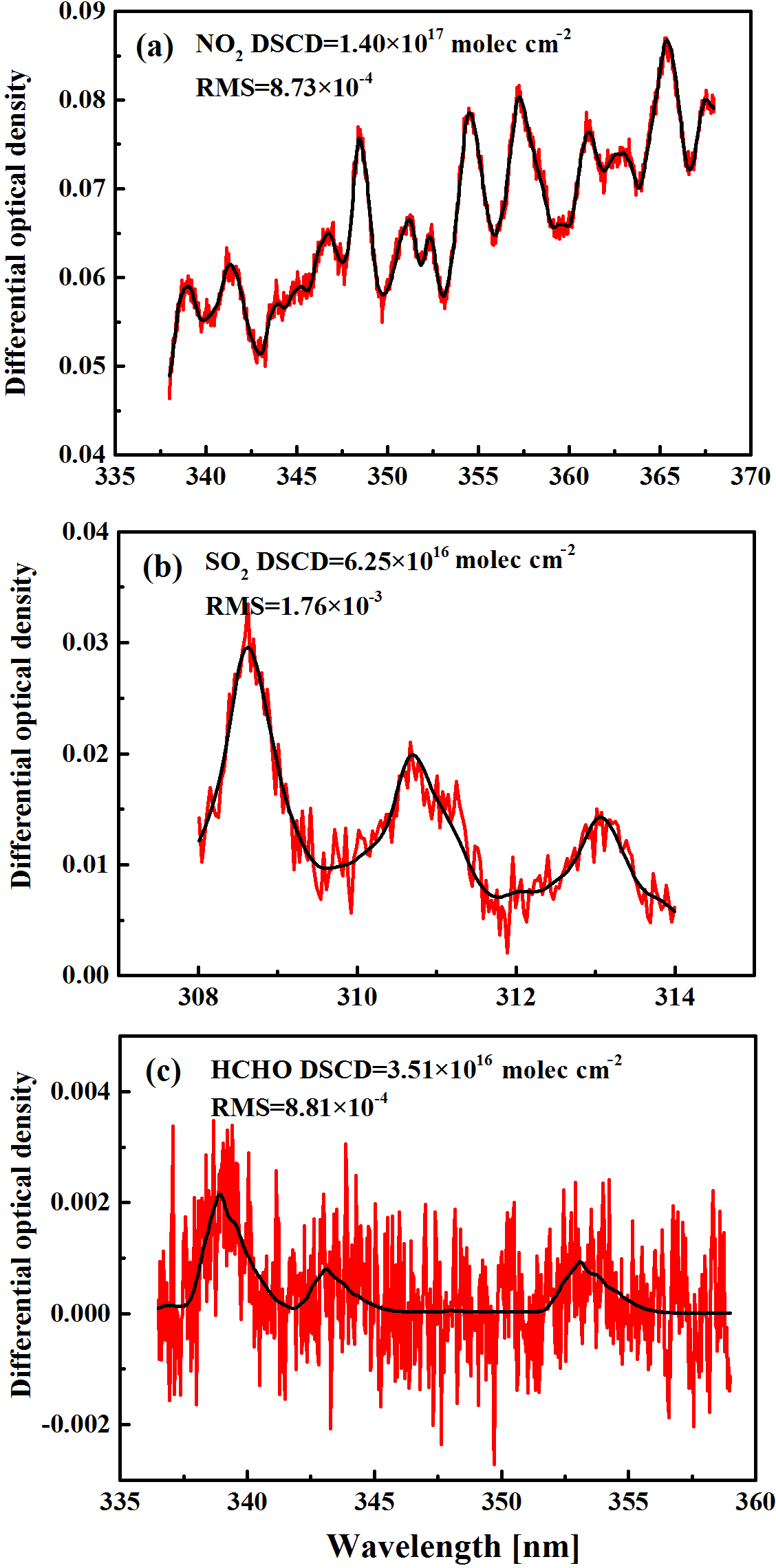
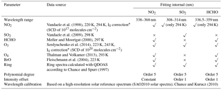
Figure 2 An example of DOAS fit for (a) NO₂, (b) SO₂, and (c) HCHO. The spectrum was taken on 1 December 2015 at 14:02 LT with an elevation angle of 30^∘. Red lines show the measured atmospheric spectrum after all other absorbers have been subtracted, and the black line shows the scaled reference absorption cross section.

Figure 2 shows an example of the DOAS analysis of a spectrum recorded on 1 December 2015 at 14:02 LT with an elevation of 30^∘. The retrieved NO₂ (Fig. 2a), SO₂ (Fig. 2b), and HCHO (Fig. 2c) DSCDs are 1.40 × 10¹⁷, 6.25 × 10¹⁶, and 3.51 × 10¹⁶ molec cm⁻², respectively. In this study, only data with a root mean square (rms) of residuals smaller than 3.0×10⁻³ are considered. This filtering criterion (rms) removed 18.7, 20.2, and 25.2 % of data for NO₂, SO₂, and HCHO, respectively.

2.2.4 Determination of the tropospheric VCD

The DOAS spectral retrieval results are the differential slant column densities (DSCDs) which are defined as the difference between the slant column density (SCD) of the measured spectrum and the Frauenhofer reference spectrum:

$$\begin{array}{}\text{(1)}& {\displaystyle }{\mathrm{DSCD}}_{\mathrm{meas}}={\mathrm{SCD}}_{\mathrm{meas}}-{\mathrm{SCD}}_{\mathrm{Fraunhofer}}.\end{array}$$

The SCD is the integrated trace gas concentration along the light path through the atmosphere, which includes both tropospheric and stratospheric part (SCD_meas = SCD_trop + SCD_strat). As scattering of photons most likely takes place in the troposphere, it can be assumed that the light paths in the stratosphere for zenith and off-zenith measurements are very similar; i.e. SCD_strat(α) ≈ SCD_strat(90^∘). Then Eq. (2) can be written as

$$\begin{array}{ll}{\displaystyle }{\mathrm{DSCD}}_{\mathrm{meas}}\left(\mathit{\alpha }\right)& {\displaystyle }=\left({\mathrm{SCD}}_{\mathrm{trop}}\right(\mathit{\alpha })+{\mathrm{SCD}}_{\mathrm{strat}}(\mathit{\alpha }\left)\right)\\ {\displaystyle }& {\displaystyle }-\left({\mathrm{SCD}}_{\mathrm{trop}}\right(\mathrm{90}{}^{\circ })+{\mathrm{SCD}}_{\mathrm{strat}}(\mathrm{90}{}^{\circ }\left)\right)\\ {\displaystyle }& {\displaystyle }={\mathrm{SCD}}_{\mathrm{trop}}\left(\mathit{\alpha }\right)-{\mathrm{SCD}}_{\mathrm{trop}}\left(\mathrm{90}{}^{\circ }\right)\\ \text{(2)}& {\displaystyle }& {\displaystyle }={\mathrm{DSCD}}_{\mathrm{trop}}\left(\mathit{\alpha }\right),\end{array}$$

where DSCD_trop(α) represents the tropospheric DSCD measured at an elevation angle of α.

As the DSCDs are measured in the atmosphere, the measurement has to be converted to vertical column density (VCD) in order that the measurements can be compared with each other. For this purpose, a concept called the air mass factor (AMF) is applied (Solomon et al., 1987), and the tropospheric VCD (VCD_trop) can be expressed as follows:

$$\begin{array}{}\text{(3)}& {\displaystyle }{\mathrm{VCD}}_{\mathrm{trop}}={\displaystyle \frac{{\mathrm{SCD}}_{\mathrm{trop}}\left(\mathit{\alpha }\right)}{{\mathrm{AMF}}_{\mathrm{trop}}\left(\mathit{\alpha }\right)}}.\end{array}$$

Assuming scattering happens above the trace gas layer, the AMF for the zenith and the off-axis view can be estimated as 1 and 1∕sinα, respectively (Hönninger et al., 2004). This method is called “geometric approximation”. However, geometric approximation of AMF could result in large errors under high aerosol load conditions (Wagner et al., 2007). In addition, the relative azimuth angle, defined as the angle between the viewing direction and the sun, also plays an important role in the AMF calculation. This effect is particularly important for mobile observations (Wagner et al., 2010). For this reason, we adapted the simultaneous lidar measurement of aerosol profiles for the radiative transfer calculation of AMFs.

In this study, AMFs for SCD to VCD conversion were calculated using the radiative transfer model SCIATRAN 2.2 (Rozanov et al., 2005). Compared to the geometric approach, radiative transfer calculation of AMF is more computationally expensive. Vertical distribution profiles of aerosols and trace gases are also important for AMF calculations. In this study, trace gas profiles (e.g., O₃, NO₂, SO₂, and HCHO) and vertical profiles of pressure and temperature are taken from the Weather Research and Forecasting model coupled with Chemistry (WRF-Chem) simulations for AMF calculations (Liu et al., 2016). Atmospheric profiles obtained from the model simulation were then interpolated in both spatial and temporal dimensions to MAX-DOAS measurements' location and time for AMF calculation. Hourly averaged aerosol extinction coefficients in the lowest 2 km of the troposphere were taken from the Mie lidar measurements, while aerosols above 2 km were not considered in the radiative transfer simulations. Aerosols below the lidar overlap height are considered to be homogeneous in the AMF calculation. In order to estimate the influence of aerosol above 2 km on the AMF calculation, we compared AMFs calculated with and without consideration of aerosols above 2 km. As the lidar measurement above 2 km has larger uncertainty, aerosols extinction information above 2 km is taken from WRF-Chem simulations. Comparison results show that AMFs calculated with considering aerosol above 2 km are on average 2–4 % lower than AMFs without consideration of aerosol at upper altitudes. The result indicates that ignoring aerosols above 2 km only causes a negligible error in the AMF calculation. Tropospheric AMFs of NO₂, SO₂, and HCHO were calculated at the central wavelength of their DOAS fitting windows, which are 354, 311, and 347 nm, respectively. The aerosol extinction profiles obtained from the Mie lidar are converted to MAX-DOAS retrieval wavelengths, assuming a fixed Ångström coefficient (Ångström, 1929) of 1. The aerosol extinction profiles at 354, 311, and 347 nm can be derived using the following formula:

$$\begin{array}{}\text{(4)}& {\displaystyle }\mathit{\alpha }({\mathit{\lambda }}_x,z)=\mathit{\alpha }({\mathit{\lambda }}_{\mathrm{532}},z)\times ({\displaystyle \frac{{\mathit{\lambda }}_x}{{\mathit{\lambda }}_{\mathrm{532}}}}{)}^{-\mathit{\upsilon }},\end{array}$$

where α (λ_x, z) is the aerosol extinction coefficient at wavelength λ_x; α (λ₅₃₂, z) is the aerosol extinction coefficient at 532 nm; and υ is the Ångström coefficient, which is assigned to a fixed value (υ=1) in this study.

A fixed set of single scattering albedo (SSA) of 0.95, asymmetry parameter (AP) of 0.68, and surface albedo of 0.06 is assumed in the radiative transfer calculations (Chen et al., 2009; Pinker et al., 1995). In this study, all radiative transfer calculations were performed by using the radiative transfer model SCIATRAN 2.2 (Rozanov et al., 2005). Previous studies show that the uncertainties caused by aerosol SSA, AP, and surface albedo assumptions are less than 10 % (Chen et al., 2009; Wang et al., 2012b). Uncertainty of lidar measurement of aerosol extinction profiles also contributes to the uncertainty in the AMF calculations. A sensitivity study was performed with aerosol profiles with different aerosol optical depths (i.e., 0.4, 0.6, 0.8, 1.0, and 1.2) and a single trace gas profile with a constant NO₂, SO₂, and HCHO concentration of 5.4 × 10¹¹ molecules cm⁻³ (equal to 20 ppb at the ground level) to quantify the uncertainty caused by aerosol profiles used in the AMF calculation at different wavelengths. In the sensitivity analysis, aerosols and trace gases are assumed to be well mixed in the lowest 0.8 km, following an exponential decrease with height. The result shows that the AMFs with different aerosol profiles (SZAs smaller than 75^∘) are 11, 13, and 11 % for NO₂, SO₂, and HCHO, respectively (see Fig. S2 in the Supplement). Considering the uncertainties caused by the assumptions of SSA, AP, and surface albedo and uncertainties of aerosol load in the radiative transfer calculations, we estimated that the uncertainties of tropospheric AMFs range between 30 and 43 % for SZAs smaller than 75^∘.

As the DOAS analysis results are DSCDs, we have to apply the concept of the differential air mass factor (DAMF) to convert the measurement to vertical columns as follows:

$$\begin{array}{ll}{\displaystyle }{\mathrm{DSCD}}_{\mathrm{trop}}\left(\mathit{\alpha }\right)& {\displaystyle }={\mathrm{SCD}}_{\mathrm{trop}}\left(\mathit{\alpha }\right)-SC{D}_{\mathrm{trop}}\left(\mathrm{90}{}^{\circ }\right)\\ {\displaystyle }& {\displaystyle }={\mathrm{VCD}}_{\mathrm{trop}}\\ {\displaystyle }& {\displaystyle }\times {\mathrm{AMF}}_{\mathrm{trop}}\left(\mathit{\alpha }\right)-{\mathrm{VCD}}_{\mathrm{trop}}\times {\mathrm{AMF}}_{\mathrm{trop}}\left(\mathrm{90}{}^{\circ }\right)\\ {\displaystyle }& {\displaystyle }\Rightarrow {\mathrm{VCD}}_{\mathrm{trop}}={\displaystyle \frac{{\mathrm{DSCD}}_{\mathrm{trop}}\left(\mathit{\alpha }\right)}{{\mathrm{AMF}}_{\mathrm{trop}}\left(\mathit{\alpha }\right)-{\mathrm{AMF}}_{\mathrm{trop}}\left(\mathrm{90}{}^{\circ }\right)}}\\ \text{(5)}& {\displaystyle }& {\displaystyle }={\displaystyle \frac{{\mathrm{DSCD}}_{\mathrm{trop}}\left(\mathit{\alpha }\right)}{{\mathrm{DAMF}}_{\mathrm{trop}}\left(\mathit{\alpha }\right)}},\end{array}$$

where DAMF is defined as the difference of air mass factor (AMF) between α ≠ 90^∘ and α = 90^∘ (DAMF_trop(α) = AMF_trop (α) − AMF_trop (90^∘)). This equation (Eq. 5) is regarded as the standard method for the determination of tropospheric trace gas VCDs from MAX-DOAS observations.

Mobile MAX-DOAS observations are strongly influenced by rapid change of air masses and radiative transfer conditions along the navigating route. The standard method (Eqs. 1 to 5) to calculate tropospheric VCDs can result in large errors. An alternative method has been suggested for mobile MAX-DOAS measurements (Wagner et al., 2010). This method has been applied in previous mobile MAX-DOAS observations (Ibrahim et al., 2010; Wu et al., 2015) and reported to be better than the standard method for mobile platforms. Therefore, we adapted the new method in this study for tropospheric VCDs' conversion. The VCD_trop can be expressed as follows (combining Eqs. 1 and 3):

$$\begin{array}{ll}{\displaystyle }{\mathrm{VCD}}_{\mathrm{trop}}& {\displaystyle }={\displaystyle \frac{{\mathrm{SCD}}_{\mathrm{meas}}\left(\mathit{\alpha }\right)-{\mathrm{SCD}}_{\mathrm{strat}}\left(\mathrm{SZA}\right)}{{\mathrm{AMF}}_{\mathrm{trop}}\left(\mathit{\alpha }\right)}}\\ \text{(6)}& {\displaystyle }& {\displaystyle }={\displaystyle \frac{\mathrm{D}{\mathrm{SCD}}_{\mathrm{meas}}\left(\mathit{\alpha }\right)+{\mathrm{SCD}}_{\mathrm{ref}}-{\mathrm{SCD}}_{\mathrm{strat}}\left(\mathrm{SZA}\right)}{{\mathrm{AMF}}_{\mathrm{trop}}\left(\mathit{\alpha }\right)}},\end{array}$$

where SZA denotes the solar zenith angle. We refer to the difference of the two unknowns SCD_ref and SCD_strat (SZA) as DSCD_offset(SZA) and this can be written as follows:

$$\begin{array}{}\text{(7)}& {\displaystyle }{\mathrm{DSCD}}_{\mathrm{offset}}\left(\mathrm{SZA}\right)={\mathrm{SCD}}_{\mathrm{ref}}-{\mathrm{SCD}}_{\mathrm{strat}}\left(\mathrm{SZA}\right).\end{array}$$

The expressions for VCD_trop in Eqs. (5) and (6) are set equal:

$$\begin{array}{ll}{\displaystyle }& {\displaystyle \frac{{\mathrm{DSCD}}_{\mathrm{meas}}\left(\mathit{\alpha }\right)-{\mathrm{DSCD}}_{\mathrm{meas}}\left(\mathrm{90}{}^{\circ }\right)}{{\mathrm{AMF}}_{\mathrm{trop}}\left(\mathit{\alpha }\right)-{\mathrm{AMF}}_{\mathrm{trop}}\left(\mathrm{90}{}^{\circ }\right)}}\\ \text{(8)}& {\displaystyle }& {\displaystyle }={\displaystyle \frac{{\mathrm{DSCD}}_{\mathrm{meas}}\left(\mathit{\alpha }\right)+{\mathrm{SCD}}_{\mathrm{ref}}-{\mathrm{SCD}}_{\mathrm{strat}}\left(\mathrm{SZA}\right)}{{\mathrm{AMF}}_{\mathrm{trop}}\left(\mathit{\alpha }\right)}}.\end{array}$$

This equation can be solved for DSCD_offset(SZA) as defined in Eq. (7):

$$\begin{array}{ll}\text{(9)}& {\displaystyle }& {\displaystyle }{\mathrm{DSCD}}_{\mathrm{offset}}\left(\mathrm{SZA}\right){\displaystyle }& {\displaystyle }={\displaystyle \frac{{\mathrm{AMF}}_{\mathrm{trop}}\left(\mathrm{90}{}^{\circ }\right)\times {\mathrm{DSCD}}_{\mathrm{meas}}\left(\mathit{\alpha }\right)-{\mathrm{AMF}}_{\mathrm{trop}}\left(\mathit{\alpha }\right)\times {\mathrm{DSCD}}_{\mathrm{meas}}\left(\mathrm{90}{}^{\circ }\right)}{{\mathrm{AMF}}_{\mathrm{trop}}\left(\mathit{\alpha }\right)-{\mathrm{AMF}}_{\mathrm{trop}}\left(\mathrm{90}{}^{\circ }\right)}}.\end{array}$$

Since DSCD_offset(SZA) is a smooth function of the SZA or time, we can fit the time series of calculated DSCD_offset (SZA or t_i) by a low-order polynomial (second-order). t_i indicates the time between the two selected measurements from one elevation sequence i. The time series of the calculated DSCD_offset(SZA) can be written as

$$\begin{array}{ll}\text{(10)}& {\displaystyle }& {\displaystyle }{\mathrm{DSCD}}_{\mathrm{offset}}\left(t_i\right){\displaystyle }& {\displaystyle }={\displaystyle \frac{{\mathrm{AMF}}_{\mathrm{trop}}(\mathrm{90}{}^{\circ },t_i)\times {\mathrm{DSCD}}_{\mathrm{meas}}(\mathit{\alpha },t_i)-{\mathrm{AMF}}_{\mathrm{trop}}(\mathit{\alpha },t_i)\times {\mathrm{DSCD}}_{\mathrm{meas}}(\mathrm{90}{}^{\circ },t_i)}{{\mathrm{AMF}}_{\mathrm{trop}}(\mathit{\alpha },t_i)-{\mathrm{AMF}}_{\mathrm{trop}}(\mathrm{90}{}^{\circ },t_i)}}.\end{array}$$

The fitted polynomial represents the approximation of DSCD_offset(t_i) and can be inserted into Eq. (8). In this way we can obtain a time series of tropospheric trace gas VCDs essentially without errors introduced by the spatio-temporal variations of the trace gas field (an example is shown in Figs. S3–S5 in the Supplement). The detailed description of the method can be found in Wagner et al. (2010).

2.3 OMI satellite observations

The Ozone Monitoring Instrument (OMI) was launched on board the NASA Earth Observing System (EOS) Aura satellite on 15 July 2004 (Levelt et al., 2006). It is a nadir-viewing imaging spectrometer measuring direct sunlight and Earth's reflected sunlight in the UV and VIS range from 270 to 500 nm. OMI aims to monitor global atmospheric trace gases' distribution with high spatial (up to 13 × 24 km) and temporal (daily global coverage) resolution. The local overpass time of OMI is between 13:40 and 13:50 (local time) on the ascending node. In this study, USTC's OMI tropospheric NO₂ product is used, which is developed based on OMI's primary product and has proven to be more suitable for the atmospheric conditions in China (Liu et al., 2016; Xing et al., 2017; Su et al., 2017). Slant column densities (SCDs) of NO₂ are retrieved by applying the DOAS fit to OMI spectra (data source: OMI Level 1B VIS Global Radiances Data product (OML1BRVG), https://disc.gsfc.nasa.gov/Aura/data-holdings/OMI/oml1brvg_v003.shtml). Separation of stratospheric and tropospheric columns is achieved by the local analysis of the stratospheric field over unpolluted areas (Bucsela et al., 2013; Krotkov et al., 2017). The OMI NO₂ SCDs are converted to VCDs by using the concept of the AMF. The AMFs are calculated based on the NO₂ and atmospheric profiles derived from WRF-Chem chemistry transport model simulations with a horizontal resolution of 20 × 20 km over eastern China (17–49^∘ N, 95–124^∘ E) and 26 vertical layers from the ground level to the height with a pressure of 50 hPa. In this study, the National Centers for Environmental Prediction (NCEP) Final operational global analysis (FNL) meteorological data are used to drive the WRF-Chem simulations. Details of the chemistry transport model simulation as well as the satellite data retrieval process can be found in Liu et al. (2016).

Figure 3 Time series of tropospheric NO₂ (a), SO₂ (b), and HCHO (c) vertical column densities (VCDs) from 22 to 28 November. The error bars refer to the 1σ variation of the measurement. Note that the data were 30 min averages, and individual measurements taken under unfavorable wind directions were filtered before averaging. No data are presented for 25 November due to frequent power outages. The y axis scale of HCHO on 26 November is different (y axis scale in red).

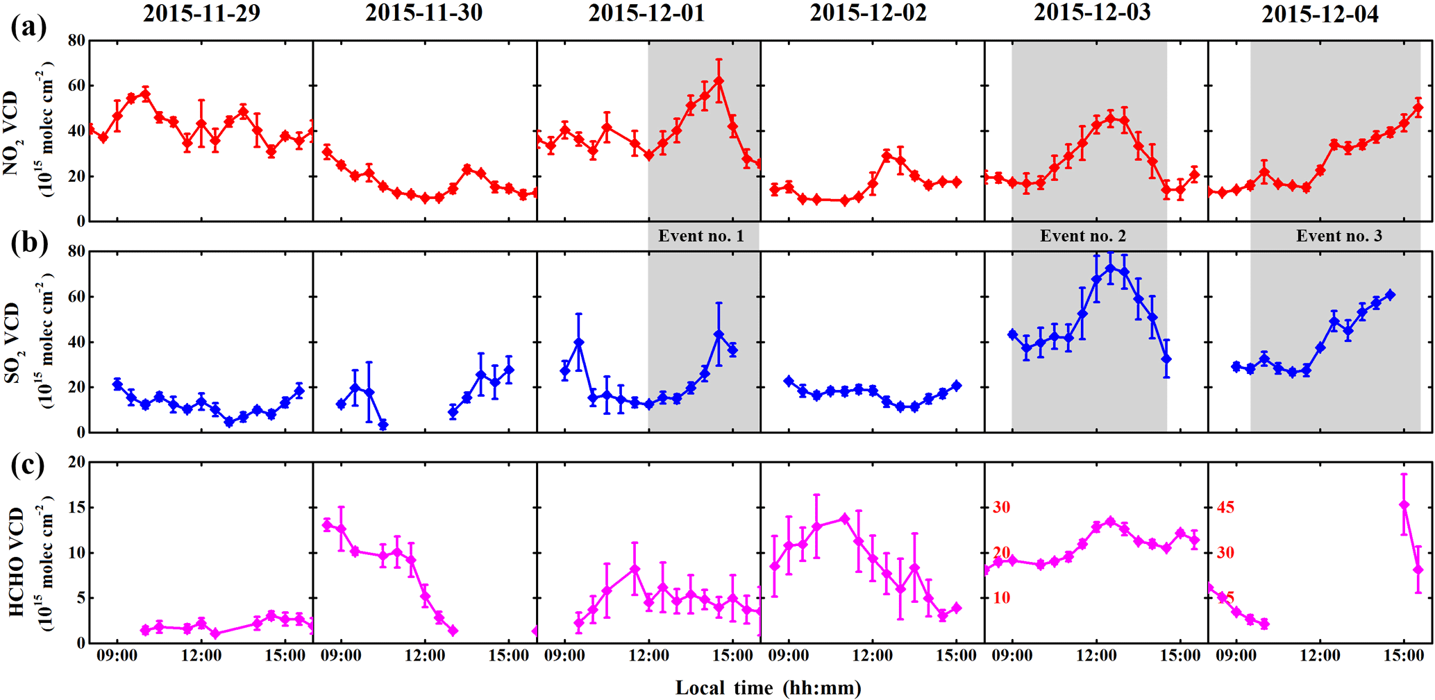
Figure 4 Continuation of Fig. 3, but for the time series of tropospheric NO₂ (a), SO₂ (b), and HCHO (c) vertical column densities (VCDs) from 22 to 28 November. The gray area highlights the episode periods in which NO₂ and SO₂ showed synchronous growth. Note that the y axis scale of HCHO on 3–4 December is different (y axis scale in red).

2.4 Ancillary data

Lidar observations of aerosol vertical distribution were also carried out during the campaign. The lidar system is equipped with a diode-pumped frequency doubled Nd:YAG laser emitting laser pulses at 532 nm. The typical pulse energy of the laser is about 20 mJ with a pulse repetition frequency of 20 Hz. The laser beam is emitted with a divergence of 1 mrad and 200 mm off-axis to the receiving telescope with a field of view of 2 mrad, resulting in an overlap height of about 195 m. A constant lidar ratio (S_p, extinction to backscatter ratio) of 50 sr was assumed in the lidar retrieval. Details of the lidar system and the data retrieval can be found in Chen et al. (2017) and Fan et al. (2018).

Meteorological parameters such as wind direction and wind speed were obtained from an automatic weather station on board the measurement ship. In situ trace gas measurements, such as CO, O₃, and NO₂ were performed using Sensor Networks for Air Quality (SNAQ) during the campaign. SNAQ is a highly portable and low-cost air quality measurement network methodology incorporating electrochemical gas sensors which can be used for high-resolution air quality studies at ppbv levels (Mead et al., 2013). CO, O₃, and NO₂ were monitored by SNAQ with a 20 s resolution, and the detection limits of CO, O₃, and NO₂ were 3 ppbv + 5 % of measured CO, 2 ppbv + 5 % of measured O₃, and 2 ppbv + 5 % of measured NO₂, respectively, and in special cases 5 % of measured values could increase to 10 %.

3 Results and discussion

MAX-DOAS measurements were conducted during the campaign period from 22 November to 4 December 2015. The measurements were interrupted occasionally due to power failure of the measurement ship and instrumental problems; details of the measurement periods are listed in Table 1. All the times reported herein are local time (LT = UTC + 8). Measurement spectra taken during daytime between 08:00 and 16:00 (SZAs smaller than 75^∘), corresponding to the period of sunshine during wintertime in China, were used for analysis. In order to avoid unnecessary uncertainties introduced during the VCD conversion, we use the radiative transfer model with lidar aerosol profiles as input for the AMF calculation to convert all the measurements to VCDs.

Figure 5 Spatial distribution of tropospheric NO₂ (a, b), SO₂ (c, d), and HCHO (e, f) VCDs along the departing route (a, c, e, from Shanghai to Wuhan) and returning route (b, d, f, from Wuhan to Shanghai). Note that the ship was anchored at Yizheng Marine department on 3 December 2015.

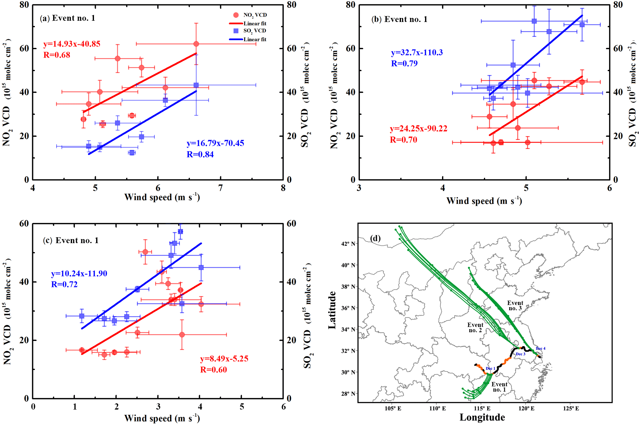
Figure 6 (a–c) Correlation analysis of ship-based MAX-DOAS VCDs (red circles show the NO₂ VCDs and blue squares show the SO₂ VCDs) and wind speed for three high VCDs events. (d) Yangtze River cruise track and 24 h backward trajectories calculated by the NOAA HYSPLIT model for three events (green marks indicate starting point: −6, −12, −18 and −24 h, respectively). The data were 30 min averages. The error bars show the 1σ of mobile DOAS VCDs and wind speed.

3.1 General characteristics of tropospheric NO₂, SO₂, and HCHO

Time series of tropospheric NO₂, SO₂, and HCHO VCDs for the entire campaign from 22 November to 4 December 2015 are shown in Figs. 3–4. Missing data are due to power failure of the measurement ship and instrumental problems, measurements taken under unfavorable wind directions, and SZAs larger than 75^∘. The mean NO₂ VCD of the entire campaign is 2.27 × 10¹⁶ molec cm⁻², with an exceptionally large variation range from 1.31 × 10¹⁵ molec cm⁻² to 7.72 × 10¹⁶ molec cm⁻². About half of the NO₂ VCDs are in the range of 5–20 (× 10¹⁵ molec cm⁻²), and high NO₂ VCDs (i.e., > 5 × 10¹⁶ molec cm⁻², approx. the 95th percentile value) are about 2.2 times higher than the mean value (Fig. S6a in the Supplement). The mean SO₂ VCD of the entire campaign is 2.14 × 10¹⁶ molec cm⁻², with a range from 1.05 × 10¹⁵ molec cm⁻² to 9.29 × 10¹⁶ molec cm⁻². Although more than half of the values are in the range of 10–25 (× 10¹⁵ molec cm⁻²), high SO₂ VCDs (i.e., > 5.5 × 10¹⁶ molec cm⁻², approx. the 95th percentile value) are about 2.5 times higher than the mean value (Fig. S6b in the Supplement). It should be noted that three elevated tropospheric NO₂ and SO₂ VCDs events have been observed which are highlighted in gray in Fig. 4. Pollution events were identified with both NO₂ and SO₂ VCDs reaching or being above the threshold value of 4.0 × 10¹⁶ molec cm⁻². The mean HCHO VCD of the entire campaign is 9.61 × 10¹⁵ molec cm⁻², ranging from 1.05 × 10¹⁵ molec cm⁻² to 5.37 × 10¹⁶ molec cm⁻². Most of the HCHO VCDs lie between 1 and 14 (× 10¹⁵ molec cm⁻²) and high HCHO VCDs (i.e., > 2.6 × 10¹⁶ molec cm⁻², approx. the 95th percentile value) are about 2.7 times higher than the mean value (see Fig. S6c in the Supplement).

Figure 7 (a) Correlation analysis and (b) time series of tropospheric NO₂ VCDs measured by ship-based MAX-DOAS and OMI during the Yangtze River campaign. MAX-DOAS data (black marks) are temporally averaged around the USTC OMI and NASA OMI overpass time (red and blue marks, respectively), while the OMI data are spatially averaged within a 20 km radius around the ship's average position. The error bars show the 1σ of ship-based MAX-DOAS and OMI data.

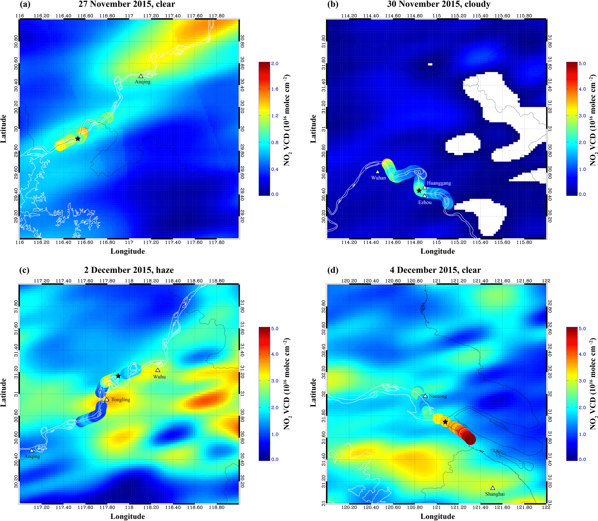
Figure 8 Spatial pattern of tropospheric NO₂ VCD measured by ship-based MAX-DOAS and OMI during four typical days within the Yangtze River campaign. The color-coded circle indicates the ship-based MAX-DOAS observations. Each plot shows examples of relatively clear (a, d), cloudy (b), and hazy (c) metrological conditions along the Yangtze River. The star symbols indicate the ship position during the OMI overpass time (∼ 13:45 LT). The color bar scale of each panel is different.

The spatial distribution of NO₂, SO₂, and HCHO VCDs along the eastern part of the Yangtze River is shown in Fig. 5. Three elevated tropospheric NO₂ and SO₂ VCD events over the Yangtze River were detected around three major industrial cities with a large number of heavy emission sources, i.e., Jiujiang (no. 1), an industrial city located on the southern shores of the Yangtze River in northwest Jiangxi Province, China, Nanjing (no. 2), the provincial capital and the most populous city in Jiangsu Province, eastern China, and Shanghai (no.3), a metropolis located in the Yangtze River Delta, with the busiest container port in the world.

The variations of the NO₂ and SO₂ VCDs are closely linked to the spatial distribution of emission sources around industrial cities as well as meteorological conditions (e.g., wind speed and wind direction). Most of the previous studies show an inverse relationship between wind speed and air quality, i.e., the lower the wind speed, the higher the pollution level, which suggests that low wind speed conditions limit the mixing and dispersion of atmospheric pollutants, and thus favor accumulation of local emissions (Chan et al., 2012, 2014, 2017; Wang et al., 2012b, 2017). However, positive correlations (p < 0.05, t test) were found between the mobile MAX-DOAS NO₂ and SO₂ VCDs (red circles and blue squares, respectively) and wind speed during these three events (Fig. 6a–c). The result suggested that these episodes are most likely not related to accumulation of local emission. We further investigated the possible influence of transport on the NO₂ spatial distribution by looking into the backward trajectories during these episodes. We calculated 24 h backward trajectories of air masses using the HYSPLIT (Hybrid Single-Particle Lagrangian Integrated Trajectory) model, which was developed by the National Oceanic and Atmospheric Administration Air Resource Laboratory (NOAA-ARL) (Stein et al., 2015) (http://ready.arl.noaa.gov/HYSPLIT.php). Meteorological data from the Global Data Assimilation System (GDAS) with a spatial resolution of 1^∘ × 1^∘ and 24 vertical levels were used in the model for the trajectory simulations. The 24 h backward trajectories (green marks indicate the trajectory point of −6, −12, −18, and −24 h) were calculated for each hour during three pollution episodes using the NOAA HYSPLIT model with an end point altitude of 500 m a.g.l. The result is shown in Fig. 6d. As indicated by the 24 h backward trajectories, NO₂ VCDs on 1 December 2015 (Event no. 1) are prominent when under southwesterly wind conditions. This is probably due to an industrial city (Jiujiang) being located on the southern shores of the Yangtze River in the upwind area of the ship. Backward trajectories (Event nos. 2 and 3, Fig. 6d) indicated prevailing northwesterly wind during 3-4 December 2015. In addition, the backward trajectory analysis suggested that rapid transport of air masses carries a significant amount of pollutants from polluted areas in northern China (Krotkov et al., 2016) across the Yangtze River, resulting in higher NO₂ and SO₂ VCDs. The higher the wind speed, the higher the NO₂ and SO₂ VCDs under northwesterly wind conditions (Fig. 6b and c), which means that the transport from distant sources is more significant than the contribution from local emission sources. These results suggested that the spatial distributions of pollutants along the Yangtze River are strongly influenced by the meteorological conditions. In comparison to these high VCDs events, relatively low NO₂ and SO₂ VCDs were observed in the first few days of the campaign (22 to 25 November), which might be due to occasional showers during these days which removed pollutants through wet deposition.

Elevated tropospheric HCHO VCDs (up to 2 × 10¹⁶ molec cm⁻²) are mostly observed during clear days (e.g., 26 November, 3 and 4 December), with good visibility and low cloud coverage (see Table 1). This is probably due to the enhancement of photochemical formation of atmospheric HCHO under strong solar irradiation. In contrast, lower HCHO VCDs were mainly observed on rainy, cloudy, and hazy days, which might be due to stronger wet deposition and weaker solar irradiation during these days. Elevated HCHO VCDs in the HCHO time series were found on 3 December 2015 when the ship was anchored at Yizheng Marine Department (32.25^∘ N, 119.15^∘ E). This day was mostly cloud-free with good visibility. In addition, HCHO VCDs show a diurnal pattern with low values in the morning and late afternoon and peaks around noontime. This diurnal pattern indicates the significant contribution of the photochemical formation of HCHO. Detailed analysis of the primary sources and secondary formation of HCHO for 3 December 2015 is shown in Sect. 3.4.

3.2 Comparison with OMI NO₂

In order to compare the ship-based MAX-DOAS measurements to OMI observations, the ship-based MAX-DOAS data are temporally averaged around the OMI satellite overpass time from 12:00 to 14:00 LT. For 22, 25, and 26 November, no MAX-DOAS data were available during the OMI overpass time due to power failure of the measurement ship and instrumental problems (see Table 1). All OMI measurements within a 20 km (ship speed: ∼ 10–20 km h⁻¹) radius of the ship's average position from 12:00 to 14:00 LT are averaged and compared to the averaged ship MAX-DOAS data. For 29 November and 1 and 3 December, no satellite observations were available at the corresponding ship's location. As a result, 7 days (23, 24, 27, 28, and 30 November and 2 and 4 December) of measurements from both OMI and ship-based MAX-DOAS are used for data comparison.

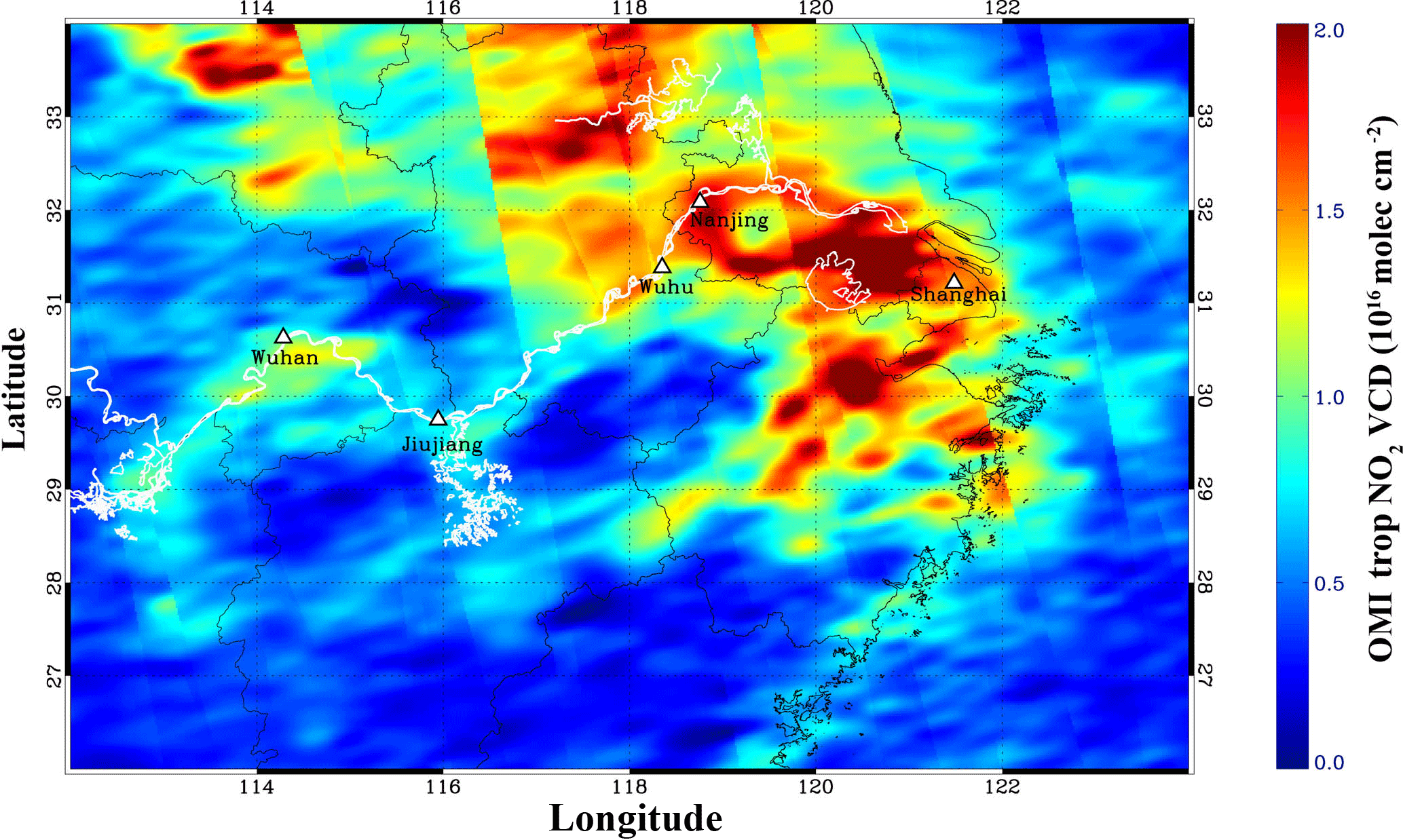
Figure 9 The spatial distribution of averaged tropospheric NO₂ VCDs measured by OMI during the Yangtze River campaign (22 November to 4 December 2015).

A scatter plot of the ship MAX-DOAS and OMI NO₂ measurements is shown in Fig. 7a. NASA's OMI NO₂ VCDs are also shown as reference. Compared to NASA's standard product, USTC's OMI tropospheric NO₂ VCD agrees better with ground measurements, with a Pearson correlation coefficient (R) of 0.82, while the correlation between MAX-DOAS and the NASA OMI product is 0.76. However, the regression analysis indicated that USTC's and NASA's OMI data underestimated the tropospheric NO₂ VCD by about 10 and 27 %, respectively. Time series of ship-based MAX-DOAS and OMI NO₂ VCDs is shown in Fig. 7b. The ship-based MAX-DOAS data were higher than the OMI values most of the time. Underestimation of tropospheric NO₂ VCDs for OMI might attribute to the averaging effect over large OMI pixels. Unpolluted or less polluted areas are also included in the OMI pixels, resulting in low values over pollution hotspots.

In order to have better insight into the spatial distribution pattern of tropospheric NO₂ along the Yangtze River, NO₂ VCDs measured by both ship-based MAX-DOAS and OMI are plotted on the same map, which is shown in Fig. 8. OMI tropospheric NO₂ VCDs are gridded onto a 0.02^∘ × 0.02^∘ grid using the parabolic spline gridding algorithm (Kuhlmann et al., 2014; Chan et al., 2015, 2017). The gridding routine was reported to provide more realistic continuous spatial distributions of NO₂ while preserving the details of emission hotspots (Chan et al., 2015, 2017). During clear days (27 November and 4 December 2015), both ship-based MAX-DOAS and OMI capture a similar NO₂ spatial pattern (Fig. 8a and d). However, a significant enhancement of NO₂ close to the estuary of the Yangtze River was observed by ship-based MAX-DOAS observations, as shown in Fig. 8d, which does not show up in the OMI observations. This is probably due to the mismatch of OMI overpass time and the ship-based MAX-DOAS measurement time. The spatial coverage of OMI observation was limited on 30 November 2015 due to cloudy sky conditions. In addition, NO₂ hotspots can be observed from the ship-based measurement as shown in Fig. 8b. These NO₂ peaks cannot be detected by OMI as clouds shield NO₂ in the lower troposphere. Different spatial patterns were detected by ship-based MAX-DOAS and OMI on 2 December 2015, which was a haze day (Fig. 8c). In order to estimate the influence of ignoring aerosols in satellite AMF calculation on NO₂ retrieval, we compared OMI NO₂ VCDs calculated with and without consideration of aerosol in the satellite AMF calculations. Significant enhancement of OMI NO₂ VCDs is observed over some areas when aerosol is considered in the satellite retrieval. However, the spatial patterns observed by ship-based MAX-DOAS and OMI are still quite different. The result indicates that the impact of aerosol could not fully explain the discrepancy between MAX-DOAS and OMI on this day. Conversely, the MAX-DOAS and OMI observations agree better during the OMI overpass time (black star in Fig. 8), and the agreement decreases when the time differences between MAX-DOAS and OMI measurements become larger. This implies a strong temporal variability of NO₂ on this day and leads to larger differences of NO₂ spatial distribution between OMI and ship-based MAX-DOAS measurements.

Ship-based MAX-DOAS is more sensitive to near-surface NO₂; however, the measurement is only limited to the area along the Yangtze River. In order to have a broader coverage of tropospheric NO₂ distribution over the Yangtze River Delta, the OMI tropospheric NO₂ product is used in this study. Figure 9 shows the averaged tropospheric NO₂ VCDs along the Yangtze River and its surrounding regions (26–34^∘ N, 112–124^∘ E). Enhanced NO₂ VCDs appeared at the estuary of the Yangtze River. This area includes southern Jiangsu, eastern Anhui, and northern Zhejiang. It is obvious that the pollution level along the Yangtze River (white line in Fig. 9) is higher than surrounding areas, especially in areas from Wuhu to Wuhan. This probably results from the fact that most of the industrial activities are concentrated along the Yangtze River as logistics are much more convenient and cost-efficient through water transportation. Our observation implies that specific emission control measures should be applied in the highly polluted industrial areas along the Yangtze River.

3.3 Possible contributions to ambient NO₂ levels

Fossil fuel consumption is a major source of anthropogenic NO_x emissions, especially in highly industrialized and urbanized regions. Industrial sources (including power plants, other fuel combustion facilities, and non-combustion processes) and vehicle emissions are the two major contributors, which together composed about 90 % of the total anthropogenic NO_x emissions in China (Huang et al., 2011; Shi et al., 2014). Understanding the individual contributions of industrial sources and vehicle exhaust to ambient NO₂ is important for designing suitable emission control strategies in polluted areas, like the Yangtze River Delta. In this study, we estimated the contribution of different emission sources to NO₂ levels along the Yangtze River by analyzing the ratio between ambient NO₂ and SO₂.

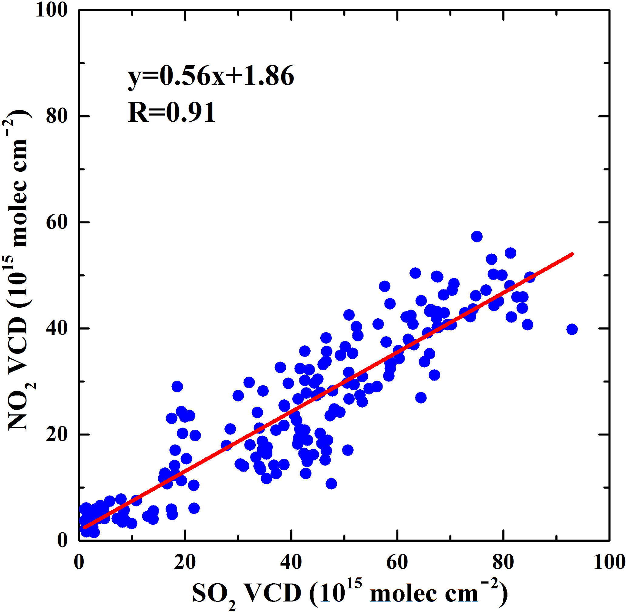
Figure 10 Scatter plot of NO₂ and SO₂ VCD data around power plants along the Yangtze River. NO₂ and SO₂ VCDs measured within 2 km of the power plants are used for the analysis.

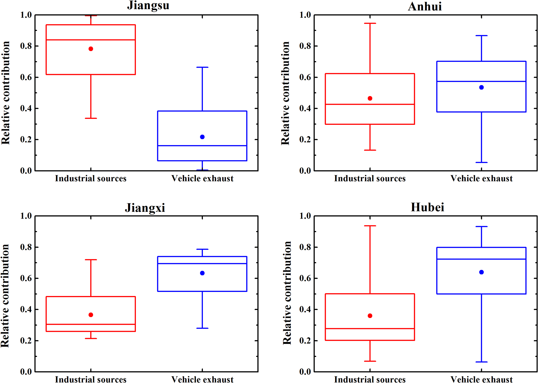
Figure 11 Relative contributions of industrial sources and vehicle exhaust to the ambient NO₂ levels over the four provinces. Note that the bottom and top of the box represent the 25th and 75th percentiles, respectively; the line within the box represents the median; the dot represents the mean; the whiskers below and above the box stand for the 10th and 90th percentiles.

Figure 1 (green dots) shows a number of power plants that are located along the Yangtze River between Shanghai and Wuhan. Industrial zones can also be found close to these power plants along the Yangtze River due to the logistical convenience. Emissions of NO₂ and SO₂ from coal-fired power plants are significant air pollution sources. As the atmospheric lifetime of NO₂ and SO₂ is roughly the same (Krotkov et al., 2016), the ambient NO₂ ∕ SO₂ ratio is approximately equal to the emission ratio of NO₂ ∕ SO₂. In addition, vehicles mainly emit NO_x and their SO₂ emissions are trivial, while coal-fired power plants, heavy industries, and ships mostly use sulfur-containing fossil fuels which emit both NO_x and SO₂. Therefore, a lower NO₂ ∕ SO₂ ratio implies a larger contribution from industrial sources (Zhang et al., 2017), while higher NO₂ ∕ SO₂ ratios indicate a larger contribution from vehicle exhaust sources toward NO₂ levels (Mallik and Lal, 2014; Krotkov et al., 2016). It should be noted that it is difficult to separate local ship emissions from industrial emissions due to their similar emission components, so industrial sources in this paper do not only include coal-fired power plants and heavy industries, but also ship emissions. In this study, we analyzed NO₂ ∕ SO₂ ratios around coal-fired power plants along the Yangtze River. NO₂ ∕ SO₂ ratios are determined by linear regression of NO₂ and SO₂ measurements around power plants, which is shown in Fig. 10. NO₂ and SO₂ VCDs measured within 2 km of the power plants (adjacent industrial zones and ships are included) are used for the analysis. Good correlation was found between NO₂ and SO₂ VCDs measured around coal-fired power plants (R = 0.91, N = 195), which implies that the ambient NO₂ and SO₂ are mostly emitted from similar sources (i.e., coal combustion). The slope of linear regression is 0.56 ± 0.02. A relatively low NO₂ ∕ SO₂ ratio indicates large contributions from combustion of high sulfur-containing fuel, e.g., coal, which is mainly used for power generation. In addition, the desulfurization filters installed in these power plants are either ineffective or maybe even deactivated during the time.

Assuming the ambient NO₂ is mostly emitted from industrial sources (mainly from power plants, and ship emissions are also included) and vehicle exhaust, other anthropogenic sources like biomass burning and natural sources are negligible. The NO₂ ∕ SO₂ ratio (slope) and intercept (offset) of the linear regression of data measured around the power plants can be used to estimate the source contributions of industrial sources and vehicle exhaust to the ambient NO₂ concentration. Assuming the NO₂ ∕ SO₂ ratio for industrial emission is constant, we can estimate the industrial and vehicle contribution by using the following equations:

$$\begin{array}{ll}{\displaystyle }{P}_{\mathrm{industrial}\mathrm{sources}}& {\displaystyle }={\displaystyle \frac{{\mathrm{NO}}_{\mathrm{2}}\left(\mathrm{power}\mathrm{plants}\right)}{{\mathrm{NO}}_{\mathrm{2}}\left(\mathrm{total}\right)}}\times \mathrm{100}\mathit{\%}\\ \text{(11)}& {\displaystyle }& {\displaystyle }={\displaystyle \frac{{\mathrm{SO}}_{\mathrm{2}}\times \mathrm{slope}+\mathrm{intercept}}{{\mathrm{NO}}_{\mathrm{2}}\left(\mathrm{total}\right)}}\times \mathrm{100}\mathit{\%}\end{array}$$

$$\begin{array}{ll}{\displaystyle }{P}_{\mathrm{vehicle}\mathrm{exhaust}}& {\displaystyle }={\displaystyle \frac{{\mathrm{NO}}_{\mathrm{2}}\left(\mathrm{vehicle}\mathrm{exhaust}\right)}{{\mathrm{NO}}_{\mathrm{2}}\left(\mathrm{total}\right)}}\times \mathrm{100}\mathit{\%}\\ {\displaystyle }& {\displaystyle }={\displaystyle \frac{{\mathrm{NO}}_{\mathrm{2}}\left(\mathrm{total}\right)({\mathrm{SO}}_{\mathrm{2}}\times \mathrm{slope}+\mathrm{intercept})}{{\mathrm{NO}}_{\mathrm{2}}\left(\mathrm{total}\right)}}\\ \text{(12)}& {\displaystyle }& {\displaystyle }\times \mathrm{100}\mathit{\%},\end{array}$$

where SO₂ represents the SO₂ VCDs, NO₂(total) denotes the NO₂ VCDs, and the slope and the intercept of the linear regression are 0.56 and 1.86 (unit: 10¹⁵ molec cm⁻²), respectively.

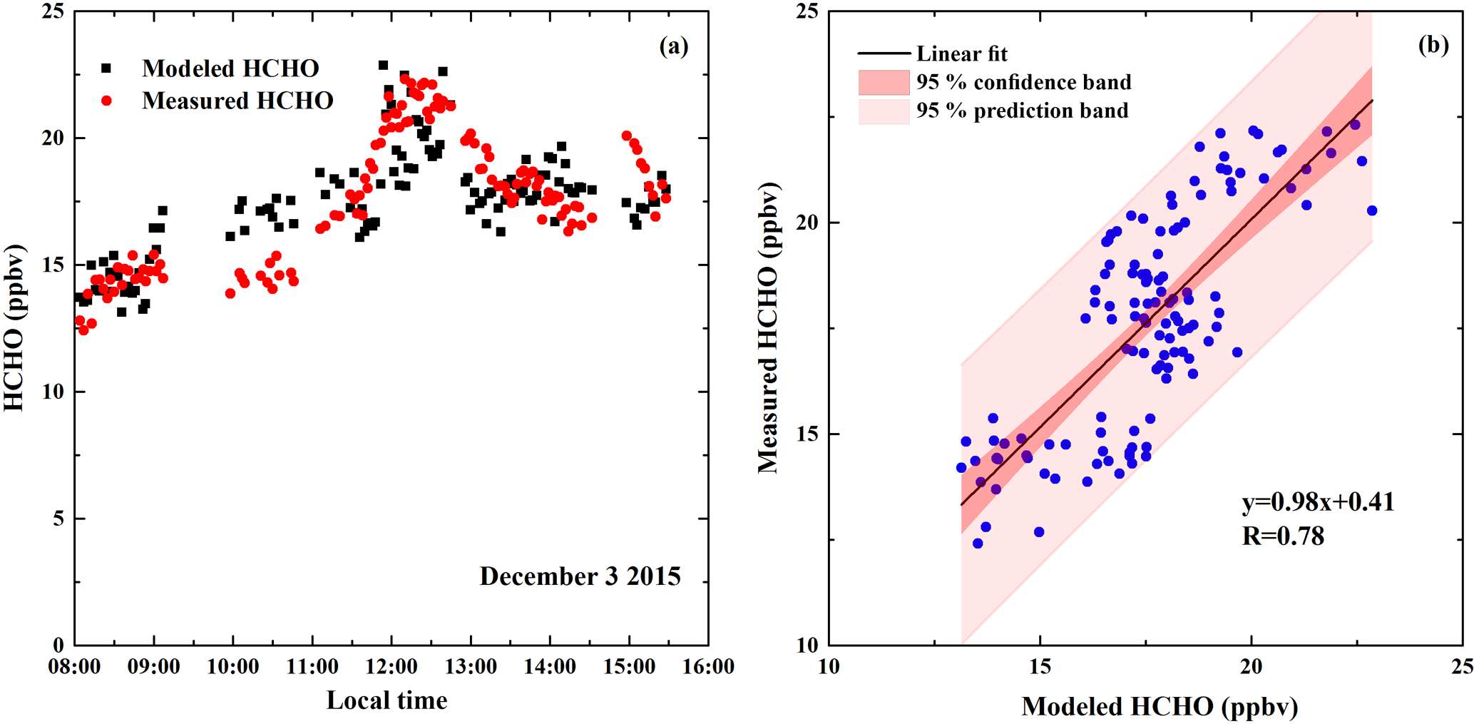
Figure 12 Comparison of the measured and modeled HCHO values from multiple linear regression on 3 December 2015. Panel (a) shows the modeled and measured HCHO time series. Panel (b) shows the linear correlation between the modeled and measured HCHO concentrations. The black solid line indicates the linear regression. The red and pink areas denote the 95 % confidence interval and the 95 % prediction, respectively.

During the campaign, the route covered four provinces along the Yangtze River, i.e., Jiangsu, Anhui, Jiangxi, and Hubei. Figure 11 shows the relative contributions of industrial sources and vehicle exhaust to the ambient NO₂ levels over the four provinces. In Jiangsu Province, a higher contribution from power generation to NO₂ levels was found, which is mainly due to the large number of power plant located along the Yangtze River in Jiangsu Province. The NO_x emission over eastern China, including Jiangsu Province (15.41 t/(km² yr)) (Shi et al., 2014), is more intensive than other parts of China. In addition, Jiangsu Province is one of the provinces in China with maximum annual NO_x emissions from coal-fired power plants (Zhao et al., 2008; Wang et al., 2012a). In contrast, the contribution of vehicle exhaust to NO₂ levels was higher than that of coal-fired power plants in Jiangxi and Hubei provinces, suggesting that traffic emissions have larger impacts on NO₂ levels in these provinces. A previous study showed how the dramatic growth of the number of vehicles has played an increasingly significant role for regional NO₂ pollution over the past years (Xia et al., 2016). For Jiangxi and Hubei provinces, the number of power plants is lower than in Jiangsu Province. Therefore, the contribution of vehicle exhaust to NO₂ level is expected to be more pronounced, corresponding with the dramatic growth of the number of vehicles. In Anhui province, the contributions of coal-fired power plants and vehicle exhaust to NO₂ level were about the same. Our result suggests that different pollution controlling strategies should be applied in different provinces: power generation emissions are the major reduction target for Jiangsu Province, while more specific control policies are needed to reduce the vehicle exhaust pollution in Jiangxi and Hubei provinces.

3.4 Estimation of primary and secondary sources of ambient HCHO

Industrial zones are mainly located along the Yangtze River due to the logistical convenience. Observations along the Yangtze River were constantly influenced by plumes originating from various industrial activities, such as coal burning, crude oil refining, and plastic and rubber syntheses. Besides the direct primary emissions, ambient HCHO can also be formed through secondary atmospheric processes. Therefore, it is important to quantify the contribution of primary and secondary HCHO in order to better understand the atmospheric processes as well as the corresponding impacts on the local air quality.

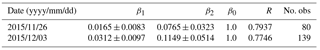
Table 3 Coefficients of the multiple linear regression and the correlation coefficient (R) for the measured and modeled HCHO in Eq. (15). β₁ represents the emission ratio of HCHO with respect to CO. β₂ denotes the portion of HCHO from photochemical production, while β₀ represents HCHO background concentration which is fixed to 1 ppbv.

CO is directly emitted to the atmosphere through combustion processes (e.g., incomplete combustion of vehicle engines) and therefore can be used as a tracer for primary emission of HCHO (Friedfeld et al., 2002; Garcia et al., 2006). In addition, O₃ reacts with NO emitted from automobiles to form NO₂. Thus, the odd oxygen O_x (O_x = O₃ + NO₂) is often used as a tracer for photochemical processes in the urban atmosphere (Wood et al., 2010). In this study, we use CO as the tracer of primary HCHO, while O_x is an indicator of secondary HCHO formation. The CO and O_x data were measured by SNAQ during this campaign. In addition, a simplified formula was used to convert mean HCHO DSCDs to mixing ratios (ppbv) (Lee et al., 2008) (detailed formula and parameters are shown in the Supplement). A previous study showed that a linear model can be used for the source appointment analysis of ambient HCHO (Garcia et al., 2006). The measured HCHO was apportioned by a multiple linear regression model, which is parameterized by the following equation:

$$\begin{array}{}\text{(13)}& {\displaystyle }\left[\mathrm{HCHO}\right]={\mathit{\beta }}_{\mathrm{0}}+{\mathit{\beta }}_{\mathrm{1}}\left[\mathrm{CO}\right]+{\mathit{\beta }}_{\mathrm{2}}\left[{\mathrm{O}}_x\right],\end{array}$$

where β₀, β₁, and β₂ are the fitting coefficients obtained from the multiple linear regression. The analysis was done on a daily basis.

The relative contributions of primary emission, photochemical formation, and atmospheric background HCHO to the total atmospheric HCHO are calculated according to the tracer concentrations and corresponding fitting coefficients by the following equations:

$$\begin{array}{}\text{(14)}& {\displaystyle }& {\displaystyle }{P}_{\mathrm{primary}}={\displaystyle \frac{{\mathit{\beta }}_{\mathrm{1}}{\left[\mathrm{CO}\right]}_i}{{\mathit{\beta }}_{\mathrm{0}}+{\mathit{\beta }}_{\mathrm{1}}{\left[\mathrm{CO}\right]}_i+{\mathit{\beta }}_{\mathrm{2}}{\left[{\mathrm{O}}_x\right]}_i}}\times \mathrm{100}\mathit{\%}\text{(15)}& {\displaystyle }& {\displaystyle }{P}_{\mathrm{secondary}}={\displaystyle \frac{{\mathit{\beta }}_{\mathrm{2}}{\left[{\mathrm{O}}_x\right]}_i}{{\mathit{\beta }}_{\mathrm{0}}+{\mathit{\beta }}_{\mathrm{1}}{\left[\mathrm{CO}\right]}_i+{\mathit{\beta }}_{\mathrm{2}}{\left[{\mathrm{O}}_x\right]}_i}}\times \mathrm{100}\mathit{\%}\text{(16)}& {\displaystyle }& {\displaystyle }{P}_{\mathrm{background}}={\displaystyle \frac{{\mathit{\beta }}_{\mathrm{0}}}{{\mathit{\beta }}_{\mathrm{0}}+{\mathit{\beta }}_{\mathrm{1}}{\left[\mathrm{CO}\right]}_i+{\mathit{\beta }}_{\mathrm{2}}{\left[{\mathrm{O}}_x\right]}_i}}\times \mathrm{100}\mathit{\%},\end{array}$$

where P_primary represents the contribution from primary sources (vehicle and industrial emissions), P_secondary is the contribution of secondary HCHO (photochemical oxidation), and P_background indicates the background HCHO, which is neither classified as primary nor secondary HCHO. According to previous studies in the YRD (Wang et al., 2015; Ma et al., 2016), the background level of HCHO is limited to 1 ppbv. Therefore, the regression parameter β₀ is fixed at 1 ppbv in this analysis. [CO]_i and [O_x]_i represent the concentrations of CO and O_x at time i, respectively. β₁ and β₂ are the regression coefficients obtained from multiple linear regression.

As other factors (e.g., meteorological conditions) can also affect the atmospheric HCHO concentration, in order to make sure that the regression model is representative for atmospheric conditions, only data fulfilling the following criteria are used in the analysis: (a) the correlation coefficient (R) is larger than 0.75 (Li et al., 2010) and (b) the significance value is lower than 0.05. Of the 12 days of measurements, only 2 days fulfill the criteria to be considered in this analysis. The parameters of the multiple linear regression fit and the linear Pearson correlation coefficient (R) for the measured and modeled HCHO are shown in Table 3.

Time series of measured and modeled HCHO of 3 December 2015 is shown in Fig. 12a. Both the measured and modeled HCHO concentrations show similar temporal development, with a rising trend in the morning, reaching a peak value at noon, and followed by a decrease in the afternoon. The linear regression between measured and modeled HCHO shows a reasonably good agreement, with a slope of 0.98 and a Pearson correlation coefficient (R) of 0.78 on 3 December 2015 (see Fig. 12b). All measurements lie within the 95 % prediction interval, indicating the best estimate of modeled HCHO. The regression model could not fully reconstruct the measurements, indicating there are other factors influencing the atmospheric HCHO levels. Due to the complexity of emission sources, a constant CO ∕ HCHO factor might not be good enough to represent the HCHO emission from all primary sources. A number of petrochemical-related manufacture and organic synthesis process industries located along the Yangtze River result in higher HCHO emissions, and the CO emission factor varies with their emission processes. In addition, as we were measuring on a mobile platform, the composition of emission could change with the measurement location. Future investigation could focus on characterizing the primary industrial emissions of HCHO by different sectors.

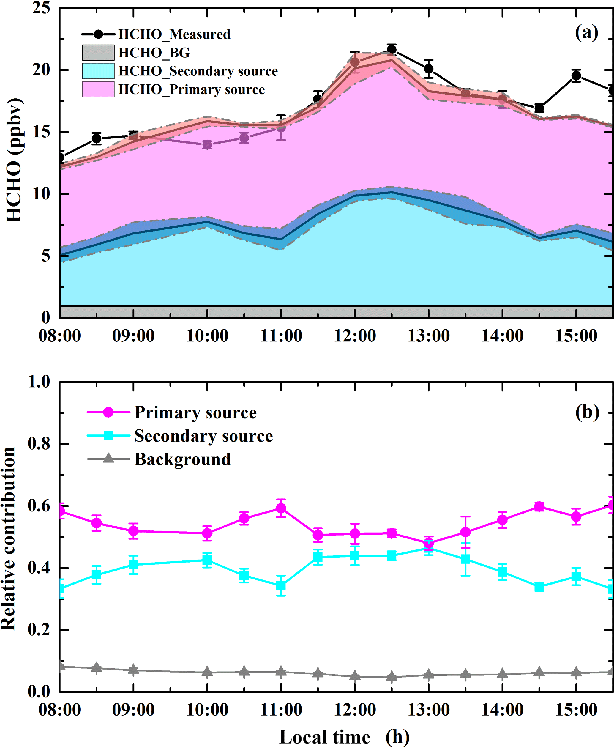
Figure 13 Time series of absolute (a) and relative (b) contribution of the primary source, secondary source, and atmospheric background to ambient HCHO levels on 3 December 2015. The error bars refer to the 1σ of the absolute (a, error bars with fill area) and relative (b) contribution of the primary source, secondary source, and atmospheric background to ambient HCHO.

The diurnal variation of HCHO contribution from primary sources, secondary formation, and background contributions on 3 December 2015 is shown in Fig. 13. Background HCHO only accounts for a small portion (6.2 ± 0.8 %, average ± SD) of the total ambient HCHO, while the primary sources contribute the largest fraction of the ambient HCHO, with an average percentage of 54.4 ± 3.7 %. The primary source contributions were relatively stable, which might be due to industrial emissions not showing a significant diurnal pattern. The contribution associated with secondary formation accounted for roughly 39.3 ± 4.3 % of the total HCHO on average daily. Secondary formation of HCHO shows two peak values around 10:00 LT and noon time (11:00–14:00 LT). The 24 h backward trajectories on 3 December (Fig. 6d) suggested that rapid transport of air masses carries a significant amount of pollutants including formaldehyde precursors from polluted areas in northern China. Thus, the peak of relative contribution of secondary sources around 10:00 LT probably resulted from the transportation of formaldehyde precursors. Additionally, the peak value of secondary formation of HCHO during noon time (11:00–14:00 LT) is mainly due to enhancement of the photochemical reaction during noon time. Our result is consistence with a similar study in Rome, Italy, for which the secondary contribution of HCHO was about 35 % during wintertime (Possanzini et al., 2002). In addition, secondary formation of HCHO has been reported as the largest ambient HCHO source in summer (Parrish et al., 2012; Ling et al., 2017). A reduced photochemical reaction in winter results in a lower formation rate of HCHO, and therefore, primary emissions become the major source of ambient HCHO in winter.

4 Summary

In this paper, we present the ship-based MAX-DOAS measurements along the Yangtze River from Shanghai to Wuhan (22 November to 4 December 2015). Scattered sunlight spectra were measured to retrieve differential tropospheric slant column densities (DSCDs) of NO₂, SO₂, and HCHO. DSCDs of NO₂, SO₂, and HCHO were converted to tropospheric vertical column densities (VCDs) using the AMF computed by the radiative transfer model, with lidar aerosol profiles as input. During the campaign, three significantly enhanced tropospheric NO₂ and SO₂ VCD events were detected over the downwind areas of industrial zones. Spatial distributions of atmospheric pollutants are strongly affected by meteorological conditions; i.e., positive correlations were found between the ship-based MAX-DOAS data and wind speed for these three events, which indicates that the transportation of pollutants from the high-emission areas has a strong influence on the NO₂ and SO₂ distribution along the Yangtze River. Comparison of tropospheric NO₂ VCDs between ship-based MAX-DOAS and OMI satellite observations shows good agreement, with a Pearson correlation coefficient (R) of 0.82. However, OMI underestimated tropospheric NO₂ by 10 %, which is mainly due to the averaging effect over large OMI pixels. In addition, satellite observations have a lower sensitivity to near-surface pollutants compared to ground-based measurements.

In this study, the NO₂ ∕ SO₂ ratio is used to quantify relative contributions of industrial sources and vehicle emissions to ambient NO₂ levels. The result shows that Jiangsu Province has a higher contribution from industrial sources due to the large number of power plants situated along the Yangtze River in Jiangsu. In contrast, contributions from vehicle emissions to NO₂ levels are higher than those of industrial sources in Jiangxi and Hubei provinces. Our result suggested that traffic volume has a large impact on NO₂ levels in these provinces. These results indicate that different NO₂ pollution control strategies should be applied in different provinces. In addition, we estimated the contributions of primary and secondary emission sources to ambient HCHO levels using a multiple linear regression method. The results from 3 December 2015 indicated that primary sources make the largest contribution to ambient HCHO (54.4 ± 3.7 %), while secondary formation contributes 39.3 ± 4.3 % of total ambient HCHO. The remaining fraction, 6.2 ± 0.8 %, is attributed to the background. The largest contribution from primary sources in winter suggested that photochemically induced secondary formation of ambient HCHO is reduced due to lower solar irradiance in winter. This study provides an improved understanding of the impacts of different emission sources in different provinces along the eastern part of the Yangtze River on the local air quality. Our findings are useful for designing specific air pollution control strategies and environmental policies.