the Creative Commons Attribution 4.0 License.
the Creative Commons Attribution 4.0 License.
 | 17 Apr 2018
Observations of ozone-poor air in the tropical tropopause layer
Richard Newton
Geraint Vaughan
Eric Hintsa
Michal T. Filus
Laura L. Pan
Shawn Honomichl
Elliot Atlas
Stephen J. Andrews
Lucy J. Carpenter
Ozonesondes reaching the tropical tropopause layer (TTL) over the west Pacific have occasionally measured layers of very low ozone concentrations – less than 15 ppbv – raising the question of how prevalent such layers are and how they are formed. In this paper, we examine aircraft measurements from the Airborne Tropical Tropopause Experiment (ATTREX), the Coordinated Airborne Studies in the Tropics (CAST) and the Convective Transport of Active Species in the Tropics (CONTRAST) experiment campaigns based in Guam in January–March 2014 for evidence of very low ozone concentrations and their relation to deep convection. The study builds on results from the ozonesonde campaign conducted from Manus Island, Papua New Guinea, as part of CAST, where ozone concentrations as low as 12 ppbv were observed between 100 and 150 hPa downwind of a deep convective complex.
TTL measurements from the Global Hawk unmanned aircraft show a marked contrast between the hemispheres, with mean ozone concentrations in profiles in the Southern Hemisphere between 100 and 150 hPa of between 10.7 and 15.2 ppbv. By contrast, the mean ozone concentrations in profiles in the Northern Hemisphere were always above 15.4 ppbv and normally above 20 ppbv at these altitudes. The CAST and CONTRAST aircraft sampled the atmosphere between the surface and 120 hPa, finding very low ozone concentrations only between the surface and 700 hPa; mixing ratios as low as 7 ppbv were regularly measured in the boundary layer, whereas in the free troposphere above 200 hPa concentrations were generally well in excess of 15 ppbv. These results are consistent with uplift of almost-unmixed boundary-layer air to the TTL in deep convection. An interhemispheric difference was found in the TTL ozone concentrations, with values < 15 ppbv measured extensively in the Southern Hemisphere but seldom in the Northern Hemisphere. This is consistent with a similar contrast in the low-level ozone between the two hemispheres found by previous measurement campaigns. Further evidence of a boundary-layer origin for the uplifted air is provided by the anticorrelation between ozone and halogenated hydrocarbons of marine origin observed by the three aircraft.
- Article
(7394 KB) - Full-text XML
-
Supplement
(1948 KB) - BibTeX
- EndNote


1.1 Background
Air entering the stratosphere in the Brewer–Dobson circulation originates in the tropical tropopause layer (TTL), a region between around 13 and 17 km altitude with characteristics intermediate between the highly convective troposphere below and the stratified stratosphere above (Holton et al., 1995; Highwood and Hoskins, 1998; Folkins et al., 1999; Gettelman and Forster, 2002; Fueglistaler et al., 2009). The TTL lies above the main convective outflow (10–13 km) and although deep convection can reach, and even overshoot, the tropopause (e.g. Frey et al., 2015), the region is not well mixed, and both radiative and large-scale dynamical processes influence its structure and composition (Fueglistaler et al., 2009). A key question about the TTL is whether deep convection is nevertheless capable of lifting very short-lived halogenated species near enough to the tropopause that their breakdown products reach the stratosphere and contribute to ozone destruction. In this paper, we use ozone measurements from a unique aircraft campaign to investigate the uplift of air from near the Earth's surface to the TTL.
The oceanic tropical warm pool in the western Pacific and Maritime Continent is marked by very warm surface temperatures (> 27 ∘C) and is therefore able to sustain widespread deep convection. Above the warm pool, a number of ozonesonde observations have shown very low ozone concentrations near the tropopause (Kley et al., 1996; Heyes et al., 2009; Rex et al., 2014; Newton et al., 2016), possibly indicative of uplift of near-surface air by deep convection. Unfortunately, accurate ozonesonde measurements in this part of the atmosphere are very difficult as the sondes produce a poorly characterized background current which can be half the measured signal in the TTL (Vömel and Diaz, 2010; Newton et al., 2016). Nevertheless, even after taking this into account, there is evidence of ozone mixing ratios < 15 ppbv occurring just below the tropopause. These are found in localized regions, or bubbles, generally associated with deep convection.
The first evidence of localized low-ozone bubbles in the TTL in the west Pacific region was provided by the Central Equatorial Pacific Experiment (CEPEX) campaign (Kley et al., 1996), where near-zero ozone concentrations were reported between the Solomon Islands and Christmas Island. These ozonesondes were affected by the background current problem, and after Vömel and Diaz (2010) reanalysed the data with a more representative background current correction, the minimum measured ozone concentration was ∼ 8 ppbv. Ozone concentrations < 15 ppbv were found by Heyes et al. (2009) in Darwin, Australia, in the ACTIVE campaign in 2005–2006, and on the TransBrom cruise of 2009 in the west Pacific (Rex et al., 2014). More recently, Newton et al. (2016) presented TTL ozone measurements as low as 12 ppbv from Manus Island, Papua New Guinea (2.07∘ S, 147.4∘ E); we discuss these measurements in more detail in Sect. 3.
Bubbles of relatively low ozone have also been observed in other parts of the world. During the TC4 campaign, anomalously low ozone concentrations of ∼ 60 ppbv were found at 14–16 km altitude in the TTL off the coast of Ecuador – typical values of ozone at this altitude in this region were measured to be ≥ 100 ppbv. These low-ozone bubbles were also shown to be a result of non-local convection followed by advection to where it was measured by the NASA DC-8 aircraft (Petropavlovskikh et al., 2010).
The mechanisms for producing low-ozone bubbles in the TTL are not fully understood. Clearly, uplift in deep convection is the underlying cause, but deep convection is a turbulent process and air entering at the surface would be expected to mix with its surroundings during ascent. Noting that the minimum ozone concentrations observed in the TTL above Darwin were too low to originate in the boundary layer locally, Heyes et al. (2009) proposed long-range transport in the TTL from a “hot-spot” region northeast of New Guinea. Newton et al. (2016) found that the minimum concentrations measured over Manus were only consistent with ozone measurements in the lowest 300 m over the island, suggesting uplift of air from near the surface to the TTL with little or no mixing (see below). Clearly, there is a need to corroborate these sporadic ozonesonde observations with other measurements and to determine how widespread these bubbles of low-ozone air are over the warm pool. This is the purpose of the present paper.
During January–March 2014, a coordinated aircraft campaign was conducted from Guam (13.44∘ N, 144.80∘ E) to measure the atmosphere over the tropical warm pool in unprecedented detail. Three aircraft were involved:
-
the NASA Global Hawk unmanned aircraft, as part of the Airborne Tropical Tropopause Experiment (ATTREX) (Jensen et al., 2017; data available in: Atlas, 2014b, Bui, 2014, and Elkins, 2014);
-
the NCAR Gulfstream V research aircraft, as part of the Convective Transport of Active Species in the Tropics Experiment (CONTRAST) (Pan et al., 2017; data available in: Atlas, 2014a, and Weinheimer, 2015); and
-
the UK Facility for Airborne Atmospheric Measurement (FAAM) BAe 146 aircraft, as part of the Coordinated Airborne Studies in the Tropics (CAST) experiment (Harris et al., 2017; data available in: Braesicke et al., 2014).
Together, these three aircraft were able to sample the tropical atmosphere from the surface to the lower stratosphere, enabling detailed measurements of the inflow and outflow of deep convection and the environment in which it formed. Of particular interest to this paper is the Global Hawk, which extensively sampled the TTL. With a typical flight range of 16 000 km and duration of up to 24 h, the aircraft continuously executed profiles between 45 000 ft (13.7 km) and 53 000–60 000 ft (16.2–18.3 km) (Jensen et al., 2017). Thus, it was able to gather a wealth of profiles of ozone and other gases through the TTL both in the Northern Hemisphere and Southern Hemisphere. The NCAR Gulfstream V aircraft sampled mainly in the Northern Hemisphere, between sea level and 15 km altitude (Pan et al., 2017), although some measurements were also made in the Southern Hemisphere, most notably on a flight to 20∘ S on 22 February 2014. The FAAM aircraft sampled the lower atmosphere, from the ground to 10 km altitude, but with most of the measurements in the boundary layer. These measurements were almost all in the Northern Hemisphere.
1.2 Article overview
In Sect. 2, we describe the instruments that were used aboard the three aircraft to collect the measurements described in this article. Section 3 provides a brief overview of the CAST ozonesonde measurements from Manus, which were described in detail in Newton et al. (2016), that provided the first evidence of the occurrence of localized low ozone concentrations during the campaign.
We then introduce the Global Hawk ozone profiles in Sect. 4, concentrating on one flight that sampled well into the Southern Hemisphere from Guam in Sect. 4.3 – this flight produced further evidence of low ozone concentrations, especially in the Southern Hemisphere portion of the flight. Within this section, we also discuss the uncertainties, and implications thereof, of the Unmanned Aircraft Systems (UAS) Chromatograph for Atmospheric Trace Species (UCATS) ozone instrument aboard the Global Hawk and how we approached the issue of noisiness in the UCATS dataset. This is followed by a brief discussion of the other ATTREX flights in Sect. 4.4.
Section 5 discusses the lower troposphere measurements that were made by the CAST and CONTRAST aircraft, providing information on boundary-layer ozone concentrations that can be used to infer the origin of low ozone in the TTL. Section 6 shows a subset of the very short-lived substances (VSLSs) that were measured using whole air samplers (WASs) aboard all three aircraft, showing the composition differences between the VSLSs in low-ozone and high-ozone cases to infer that recently convected ozone-deficient air has a distinct chemical composition compared to high-ozone cases. (A section in the Supplement contains the full dataset of WAS VSLS chemical data.) Finally, Sect. 7 summarizes the findings of this article.
Ozone was measured in situ by all three aircraft in the CAST, CONTRAST and ATTREX campaigns. The FAAM BAe 146 carried a Thermo Fisher Model 49C UV absorption photometer, which had an uncertainty of 2 % and a precision of 1 ppbv for 4 s measurements (Harris et al., 2017). Ozone on the Gulfstream V aircraft was measured using the NCAR chemiluminescence instrument, which uses the chemiluminescent reaction between nitric oxide and ozone. The detection limit was below 0.1 ppbv and its accuracy within 5 % for the entire range of ozone measurements made during CONTRAST (Ridley et al., 1992; Pan et al., 2015, 2017).
On the Global Hawk, the UCATS instrument provided measurements of ozone, plus nitrous oxide (N2O), sulfur hexafluoride (SF6), hydrogen (H2), carbon monoxide (CO) and methane (CH4) (Jensen et al., 2017). Ozone in the UCATS unit is measured by two Model 205 UV photometers from 2B Technologies (Boulder, Colorado) modified for high-altitude operation. The first was mounted inside the UCATS package, whilst a second, newer Model 205 photometer was added to the front panel of the UCATS. Both instruments were modified to include stronger pumps (KNF model UNMP-830), scrubbers with magnesium oxide (MgO) coated screens and pressure sensors with a range from 0 to > 1000 hPa (Honeywell ADSX series). The model 205 is a two-channel photometer, with the flow continuously split between the unscrubbed (ambient) air into one cell and scrubbed (ozone-free) air into the other for measurement by the Beer–Lambert law absorption of 253.7 nm radiation from a Hg lamp. Flow is switched every 2 s, and data are recorded at this rate for the newer instrument but averaged to 10 s in the older model. The instruments were calibrated on the ground against a NIST-certified calibration system (Thermo Electron, Inc.) before and after the mission. In both cases, the slope of the regression line between the instrument and calibrator data was within 1 % of unity and the offset less than 2 ppbv (usually < 1 ppbv) at ambient pressure and room temperature. However, in-flight comparisons on earlier ATTREX missions between the 2B instruments and the NOAA ozone photometer (Gao et al., 2012) revealed a possible negative bias of up to 5 ppbv at low ozone concentrations.
In addition to ozone data, selected WAS data are used to identify convective influence. Whole air samplers were aboard all three aircraft, measuring a large array of compounds. All three aircraft measured dimethyl sulfide ((CH3)2S), iodomethane (CH3I), dichloromethane (CH2Cl2), bromochloromethane (CH2BrCl), trichloromethane (CHCl3), dibromochloromethane (CHBr2Cl) and tribromomethane (CHBr3). The WAS samples collected aboard the BAe 146 were analysed typically within 72 h of collection, with gas chromatography – mass spectrometry (GC-MS; Agilent 7890 GC, 5977 Xtr mass selective detector, MSD) (Andrews et al., 2016; Harris et al., 2017). The CONTRAST and ATTREX whole air samples were analysed for a much larger array of compounds and were also analysed by the GC-MS. The samples were split between an Agilent HP-AL/S PLOT (porous layer open tubular) column with a flame ionization detector, and the remaining sample was split again between an electron capture detector and an Agilent 5975 GC-MSD (Schauffler et al., 1999; Apel et al., 2003; Andrews et al., 2016).
A total of 33 ozonesondes were launched from Manus Island during February 2014 as part of CAST. A salient result of the campaign was further insight into the background current: where this quantity was ≲ 50 nA, a constant offset was subtracted from the measured current, but when the background current was larger, a hybrid correction was applied which decreased with height (Newton et al., 2016). These procedures gave good agreement with nearby ozone measurements on the Gulfstream V on 5 and 22 February, verifying the use of ozonesondes to measure very low ozone concentrations near the tropical tropopause.
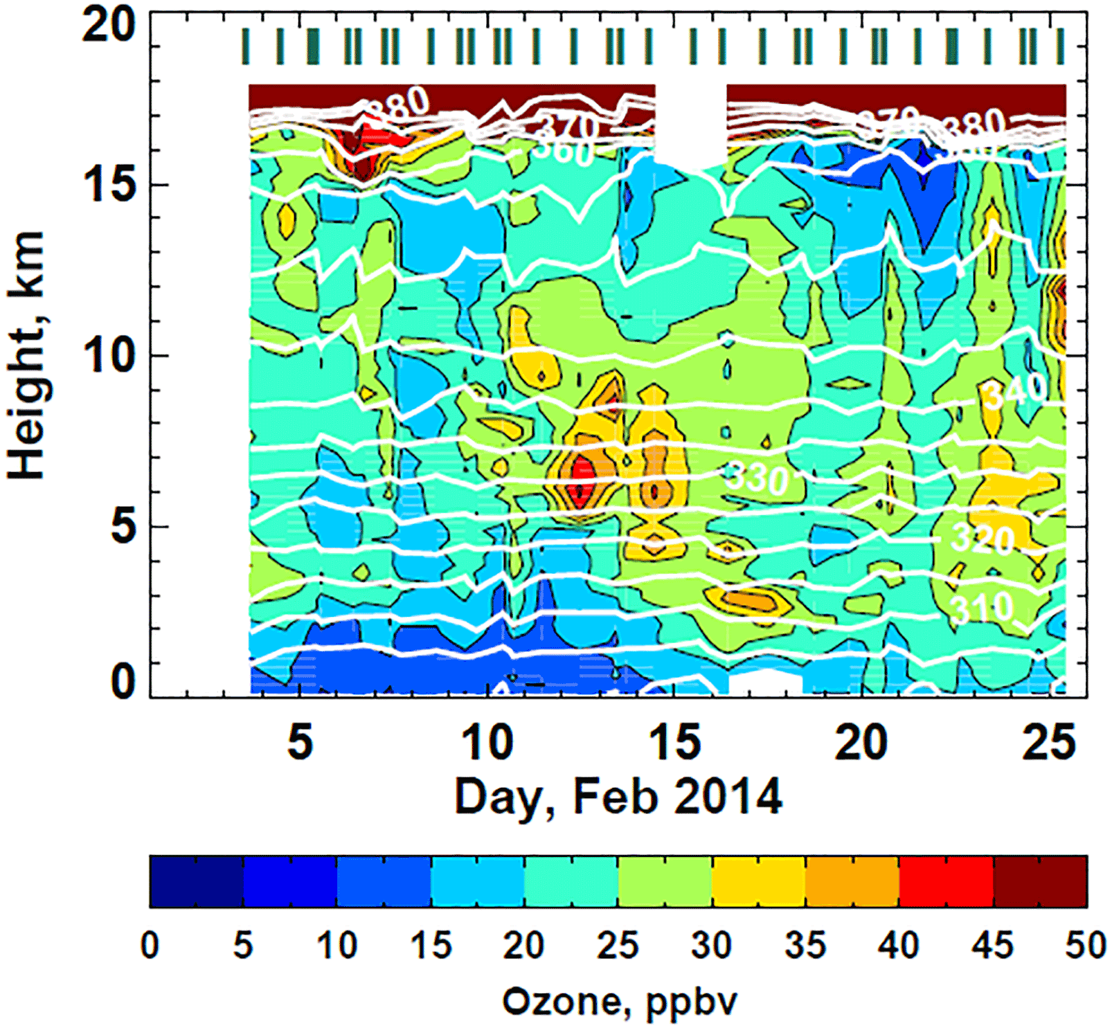
Figure 1Contour plot of ozone concentrations from the Manus ozonesondes. The white lines are potential temperature isolines. Note the very low concentrations in the upper troposphere around 21–22 February. Green bars along the top denote launch times of ozonesondes. For further details, see Newton et al. (2016).
Another salient result from the ozonesonde measurements was the low-ozone event in the TTL between 18 and 23 February, visible in Fig. 1, where measured ozone was as low as 12 ppbv. As Folkins et al. (2002) argued, the only region of the tropical troposphere able to generate ozone concentrations ≤ 20 ppbv is near the surface, so this air mass is likely to be of recent boundary-layer origin. Ozone concentrations through most of the boundary layer over Manus in this period were higher than in the TTL; only in the bottom 300 m of the profiles did the ozonesondes measure < 20 ppbv, with concentrations at the ground around 8–15 ppbv (Newton et al., 2016). This suggests either that the ozone-poor air was lifted from near the surface or that boundary-layer ozone concentrations in the uplift region were lower than over Manus. A back-trajectory analysis of the low-ozone bubble with the online Hybrid Single-Particle Lagrangian Integrated Trajectory (HYSPLIT) model (Stein et al., 2015) indicated that the origin of the low concentrations of ozone was a mesoscale convective system to the east of Manus Island that uplifted air from the lower troposphere into the tropopause layer (see Fig. 2), combined with a strong easterly jet that advected the air towards Manus Island. Unfortunately, ozone measurements were not available in this area at this time so the altitude from which the ozone-poor air was lifted remains an open question. To examine whether further examples of ozone-poor layers were encountered during the CAST/CONTRAST/ATTREX campaigns, we now examine the Global Hawk observations in the TTL during February and March 2014.
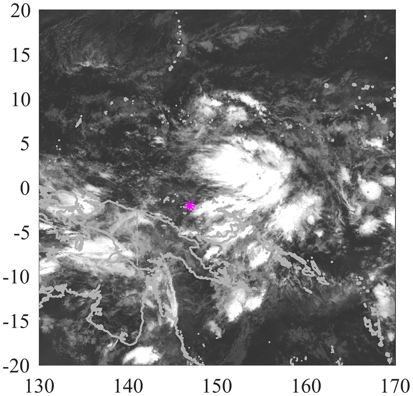
Figure 2Multi-Functional Transport Satellite (MTSAT) infrared satellite image from 19 February 2014 at 18:00 UTC, showing the convection to the east of Manus Island (pink asterisk) that was determined to be the origin of the low-ozone air in the TTL above Manus.
4.1 ATTREX flights
The Global Hawk measured in the same altitude range as the layer of ozone-poor air above Manus Island: the aircraft performed ascents and descents between 150 hPa (13.6 km) and 100–75 hPa (16.1–18.0 km), depending on fuel load. The ascent rate was slow, of the order of 45 min, to complete at an average vertical velocity of ∼ 0.5 m s−1, but the descent rate was much quicker, of the order of 5–10 min, to complete at ∼ 4 m s−1. Only the ascent data are used in this study as the descent was found to be too quick for reliable ozone measurements.
In total, six research flights were flown by the Global Hawk from Guam during the ATTREX campaign. The first two, RF01 and RF02, were on 12 and 16 February when the CAST and CONTRAST campaigns were active, but there was a gap of 15 days between the second and third flights as the aircraft developed a problem; the final four flights, RF03, RF04, RF05 and RF06 were on 4, 6, 9 and 11 March, respectively – after CAST and CONTRAST had finished. The transfer flight from Armstrong Flight Research Center in California to Andersen Air Force Base in Guam on 16 January and the return flight on 13 March made few measurements in the west Pacific region and are not considered here.
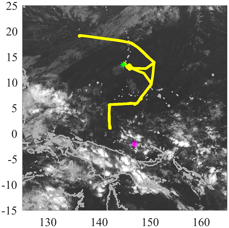
Figure 3MTSAT infrared satellite image from 12 February at 12:00 UTC, coincident with flight RF01 (yellow track). Green asterisk denotes location of Guam; magenta asterisk denotes that of Manus Island. Convection is centred mostly around the Maritime Continent on this day.
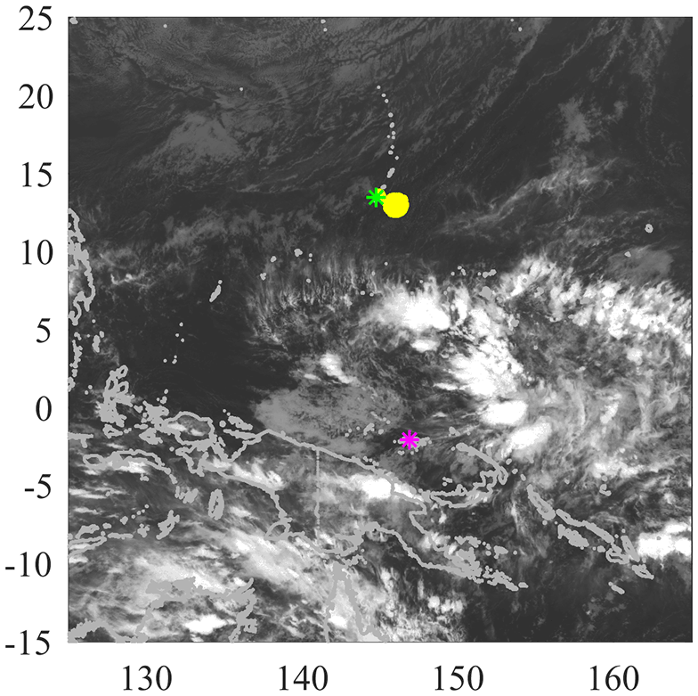
Figure 4As Fig. 3 but for 16 February at 12:00 UTC, coincident with flight RF02. A band of convective activity is visible to the southeast of Guam.
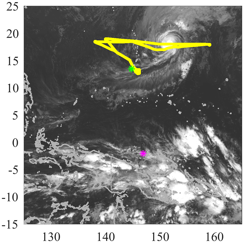
Figure 5Satellite image of 4 March at 12:00 UTC, coincident with flight RF03. Cyclone Faxai is visible to the northeast of Guam.
Flight RF01 on 12–13 February focused on the composition, humidity, clouds and thermal structure of the Northern Hemisphere part of the warm pool region. Convection was situated mostly around the Maritime Continent on this day (Fig. 3), with no notable convection around Guam. The second flight, RF02, occurred on 16–17 February with similar scientific objectives to RF01. As a result of a satellite communications problem, the aircraft was required to stay in line-of-sight contact with the air base in Guam, and consequently the aircraft flew in a small area of airspace close to the island. On this day, convection was visible to the southeast of Guam in the Multi-Functional Transport Satellite (MTSAT) satellite imagery (Fig. 4).
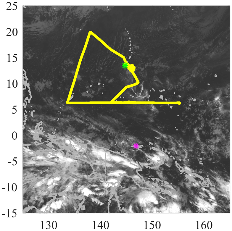
Figure 6Satellite image of 6 March at 12:00 UTC, coincident with flight RF04. Convection is minimal in the Northern Hemisphere and is concentrated mostly in the Southern Hemisphere.
The third flight took place after a 2-week hiatus on 4–5 March. Its objectives were to sample the outflow of Tropical Cyclone Faxai, which developed in the region in the previous few days, with vertical profiles performed to observe the outflow cirrus cloud from the cyclone. Apart from Tropical Cyclone Faxai, the majority of the convection was in the Southern Hemisphere around Papua New Guinea (Fig. 5).
Flight RF04 took place on 6–7 March. Tropical Cyclone Faxai had dissipated by this time, leaving a dearth of convection in the Northern Hemisphere; the most convectively active region was around Papua New Guinea (Fig. 6). RF05 surveyed the Southern Hemisphere on 9–10 March, measuring the lowest ozone concentrations observed by the Global Hawk during the ATTREX campaign. This flight is discussed in detail in the next section. The final research flight, RF06, took place on 11–12 March, surveying latitudes north of 10∘ N on either side of the subtropical jet, and is outside the scope of this paper. A full description of the ATTREX flights and meteorological conditions encountered can be found in Jensen et al. (2017).
4.2 Systematic errors in ATTREX ozone data
As discussed in Sect. 2, previous studies have suggested there may be a low bias in UCATS ozone measurements. Fortunately, flight RF02 on 16–17 February offered an opportunity to examine data from this campaign for any evidence of such a bias. As shown in Fig. 4 (and later, Fig. 16), the entire flight took place just southeast of Guam, within an area spanning 1∘ in latitude and longitude.
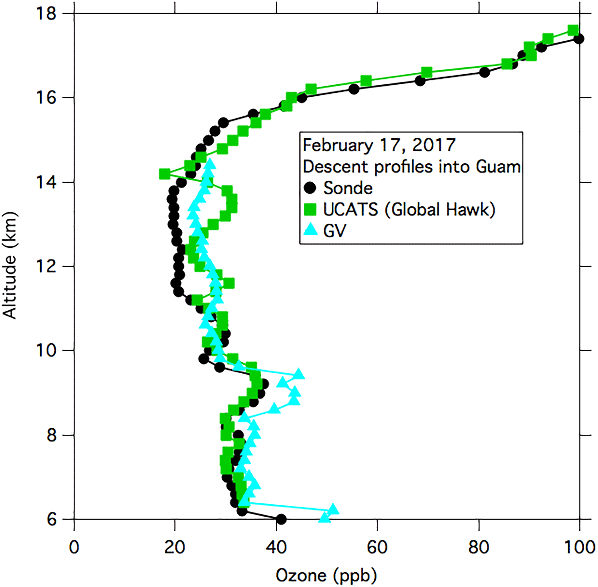
Figure 7Intercomparison of UCATS descent ozone profile on RF02 with nearby profiles from the Gulfstream V and an ozonesonde. The Global Hawk profile was measured between 09:20 and 10:45 UTC, the sonde between 08:46 and 10:44 UTC and the Gulfstream V between 05:02 and 05:23 UTC.
Figure 7 shows a comparison between UCATS data measured on the descent to Guam, the descent profile from the Gulfstream V (around 5 h earlier) and the descent profile from an ozonesonde coincident in time with the Global Hawk descent. (The ozonesondes were flown with a valved balloon, allowing both ascent and descent rates to remain below 6 m s−1, thus enabling ozone measurements on descent.) The UCATS ozone follows the descent sonde profile closely below 10 km, but in the region of lowest ozone concentration, between 12 and 14 km, it tends to be more consistent with the Gulfstream V, although showing rather more structure than the other two profiles.
Given the obvious variability in tropospheric ozone shown by Fig. 7, a quantitative validation of the UCATS ozone would require many more comparisons. We can conclude however that there is no evidence from this example of a low bias in the UCATS measurements at low concentrations. This allows measurements across the tropical warm pool by the Global Hawk to be used to explore regions of very low ozone concentration.
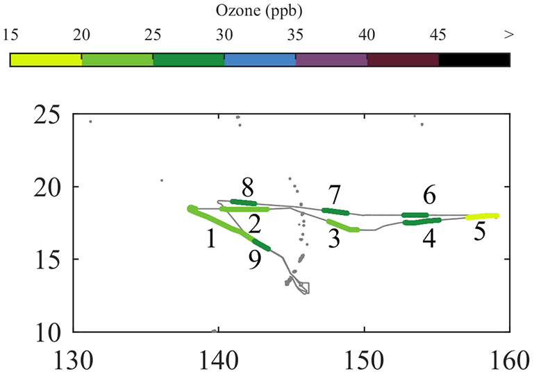
4.3 ATTREX flight RF05
ATTREX RF05 surveyed into the Southern Hemisphere on 9–10 March, sampling the outflow of strong convection along the South Pacific Convergence Zone (SPCZ). The aircraft took off at 15:30 UTC on 9 March and flew a straight path southeast, reaching its furthest point away from Guam at 00:30 UTC on 10 March before returning on a path closer to the Solomon Islands and Papua New Guinea. The aircraft returned to the vicinity of Guam at around 08:00 UTC and flew around the island before landing at 11:00 UTC. Figure 8 shows the altitude of the aircraft during RF05: after the initial ascent, there were basically 18 repeats of a relatively rapid descent, a short level section near 14.5 km and relatively slow ascent (with the exceptions that there was no level section in set 10 and the aircraft descended to Guam after the final level section).

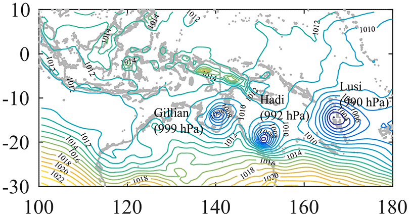
Figure 9Synoptic chart from ECMWF ERA-Interim data from 10 March at 00:00 UTC. The three tropical cyclones are labelled, along with their central minimum pressure.
Large amounts of convection were present in the southern hemispheric portion of the warm pool region around the time of ATTREX RF05. A series of tropical cyclones are shown in the synoptic analysis chart in Fig. 9: Tropical Cyclone Gillian in the Gulf of Carpentaria, Tropical Cyclone Hadi near the east coast of Queensland and Tropical Storm Lusi which was intensifying to become a tropical cyclone near the Solomon Islands on 10 March.
Before examining the Global Hawk ozone measurements in a meteorological context, account needs to be taken of noise in the UCATS data. Ozone measurements from the level sections (Fig. 8) were first examined to determine the random measurement error. The combined histogram of the departures from the mean along each level section is shown in Fig. 10; this approximates well to a Gaussian distribution with standard deviation 3.69 ppbv, suggesting that instrumental random errors in UCATS may be reduced by averaging the data.

Figure 10Histogram of departures of UCATS ozone measurements from the mean along each level section of flight.
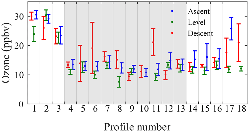
Figure 11Means and 1σ standard errors of UCATS ozone along the different sections of RF05. Shading denotes profiles in the Southern Hemisphere.
As the standard deviation is so large compared with the background ozone values in low-ozone bubbles (< 15 ppbv), there is little to be gained from trying to identify individual structures in the ascent and descent profiles. Instead, the approach used here is to average all the data in the troposphere above 14 km along an individual ascent or descent. This requires a definition of the tropopause, taken to be the lowest altitude above which ozone increases by 20 ppbv within a 5 hPa span, and continues to increase thereafter to > 50 ppbv. The result of averaging the data along each flight section in this way is shown in Fig. 11. To calculate the error bars, consideration needs to be given to real variations of ozone along the profiles, which affect the statistical independence of the measurement points. The method described by Wilks (1995, p. 127) was used to calculate the effective number of independent points N′:
where N is the number of data points along a section and ρ1 is the lag-1 autocorrelation of the data along that section. The standard error in the mean was then calculated as , where σ was the standard deviation for that section.
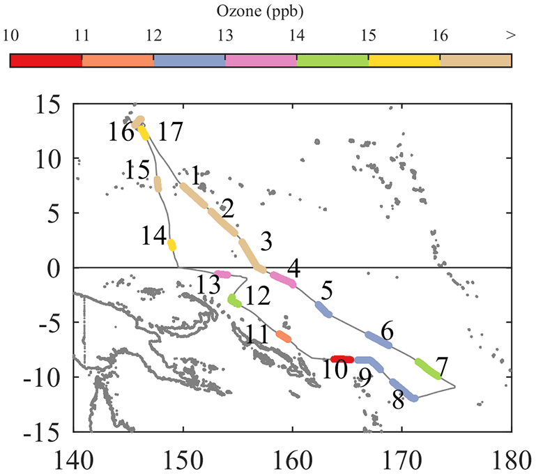
Figure 12Flight track of RF05, with each ascent profile performed by the Global Hawk chronologically numbered and coloured by mean tropospheric ozone in each profile. The length of each coloured profile corresponds to the time the aircraft was below the tropopause in that section.
The three sets of points shown in Fig. 11 are independent of one another and show a consistent pattern. For the first three sets, all the means were above 20 ppbv, with a sharp fall to < 15 ppbv in set 4. The means along the level sections remained below 15 ppbv thereafter, but the ascent and descent averages show an increase towards the end of the flight. As expected given the slower ascents and faster descents, error bars for the descents tend to be larger than for the ascents for most of the profiles. Averages along the ascent profiles therefore provide the most precise and representative measures of the mean TTL ozone concentration along the flight path, with a typical standard error of 2 ppbv. We now examine these means in a meteorological context.
Mean concentrations derived from the ascent profiles during RF05 are shown in Fig. 12, where it can be seen that the mean tropospheric ozone concentrations are lowest in the Southern Hemisphere, typically between 10 and 13 ppbv. These values are very similar to those measured in the TTL over Manus between 18 and 23 February. In the Northern Hemisphere, ozone concentrations on the return leg (between 06:00 and 08:30 UTC on 10 March) were ∼ 15–16 ppbv on average, compared to the outbound leg (between 15:45 and 19:45 UTC on 9 March), which were above 30 ppbv.
The relationship between the appearance of the low concentrations of ozone and areas of deep convection was investigated using the Met Office's Numerical Atmospheric-dispersion Modelling Environment (NAME) (Jones et al., 2007). NAME is a Lagrangian model in which particles are released into 3-D wind fields from the operational output of the UK Met Office Unified Model meteorology data (Davies et al., 2005). These winds have a horizontal resolution of 17 km and 70 vertical levels, which reach ∼ 80 km. In addition, a random walk technique was used to model the effects of turbulence on the trajectories (Ryall et al., 2001). The NAME model was used in single-particle mode, initializing one trajectory at each point along the RF05 flight track where an ozone measurement was made. Back trajectories were run for 1 day, with output at 6 h intervals.
NAME suggests that the Southern Hemisphere air originated from the southeast, in the area where Tropical Cyclone Lusi was situated. Figure 13 shows the start points of the back trajectories initialized in the troposphere (below 100 hPa) along the flight track of RF05: sections of track from which back trajectories crossed the 800 hPa isobaric surface are shown in cyan; sections where they did not are in magenta. The yellow markers denote the final position, after 24 h, of the back trajectories that crossed the 800 hPa isobaric surface, indicative of rapid convection. The majority of these trajectories are in the southern hemispheric portion of the flight and are projected by NAME to originate from Tropical Cyclone Lusi. It should be noted that the NAME model cannot capture the effect of individual convective cells because of the low horizontal resolution of the meteorological data, but its convection parameterization is capable of reproducing net vertical transport over relatively large areas (Ashfold et al., 2012; Meneguz and Thomson, 2014).
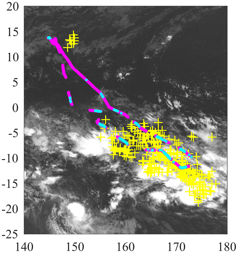
Figure 13MTSAT infrared satellite image at 18:00 UTC on 8 March 2014, around 24 h before the midpoint of flight RF05 to coincide with the endpoints of the 24 h back trajectories. Tropical Storm Lusi is visible as the cluster of convection centred around 170∘ E, 20∘ S. The tropospheric (> 100 hPa) portion of the flight track of RF05 is shown in magenta and, in the case where trajectories crossed the 800 hPa isobaric surface, in cyan. The positions after 24 h of the trajectories that crossed the 800 hPa isobaric surface at some point in the model are marked as yellow crosses.
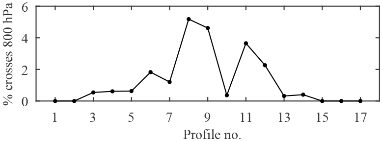
Figure 14Percentage of back trajectories crossing the 800 hPa surface within 1 day from the different ascent profiles on RF05.

Figure 15Flight track of RF01 with each profile coloured by mean tropospheric ozone as in Fig. 12. The profiles that would otherwise be obscured by other profiles are shown on the right-hand plot.
The back trajectories initialized in the Northern Hemisphere also came from the southeast, but in the 24 h period of the NAME model run, the trajectories had only reached the edge of the tropical storm, so the sampled air mass passed through this region whilst the storm was developing, rather than when it was mature.
Figure 14 shows the number of back trajectories that crossed the 800 hPa isobaric surface. None of those initialized from the Northern Hemisphere profiles 1, 2, 15, 16 and 17 crossed 800 hPa, and fewer than 1 % from profiles 3, 4, 5, 13 and 14 did so. However, up to 5 % of back trajectories initialized along profiles 6–12 in the Southern Hemisphere cross the 800 hPa isobaric surface, with exception of profile 10. These are also the sections with the lowest ozone concentrations, with values similar to those observed by the ozonesondes over Manus. Again, the low concentrations are consistent with recent uplift in deep convection.
4.4 Other ATTREX flights
The other research flights observed no notably low ozone concentrations in the tropical tropopause layer, hinting that the lowest ozone concentrations were confined to the Southern Hemisphere during the ATTREX campaign. RF01 flew in an arc, approximately following the streamlines of the monsoon anticyclone, which, along with most of the convection that day, was situated a long way to the west of Guam. Ozone concentrations on this flight were high, and none of the profiles had mean tropospheric concentrations below 45 ppbv (Fig. 15). Likewise, RF02, which flew within a small circle of airspace for the duration of its 17.5 h flight providing repeated measurements of the same air mass, observed mean ozone concentrations of 25–40 ppbv (Fig. 16).
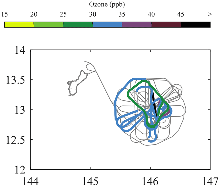
Figure 16Flight track of RF02 with each profile coloured by mean tropospheric ozone as in Fig. 12. Of the 12 profiles taken, two profiles have mean ozone concentrations of 25–30 ppbv, seven have 30–35 ppbv, and two have 35–40 ppbv.
RF03 flew eastwards to intercept the outflow of Cyclone Faxai, before returning on a similar flight track back to Guam. Mean ozone concentrations decreased below 20 ppbv on one occasion (19.5 ppbv in profile 5 – Fig. 17), but no other examples of low ozone concentrations were observed, even in the vicinity of Faxai.
RF04 flew in similar meteorological conditions as RF03, except for the dissipation of Faxai between the two flights. The flight track took the aircraft from Guam south to 6∘ N, where it performed a constant altitude flight along this line of latitude from 155 to 135∘ E before travelling northwards and back to Guam. Similar to RF03, only one profile – 16.1 ppbv in profile 1 – had mean tropospheric ozone concentrations below 20 ppbv.
RF06 flew north into the extratropics where ozone concentrations are significantly higher and is therefore not reproduced here.
In summary, an examination of the ATTREX flight data found mean upper tropospheric ozone concentrations as low as 10 ppbv in the outflow of Cyclone Lusi in the Southern Hemisphere during flight RF05, but a corresponding flight in the Northern Hemisphere in the outflow of Cyclone Faxai found the lowest mean ozone concentration to be 17.5 ppbv. Meanwhile, the FAAM aircraft measured boundary-layer concentrations around 10–12 ppbv between 1∘ S and 3∘ N on 4 February in a flight south from Chuuk along 152∘ E, values which are consistent with the Manus boundary-layer measurements at that time (Fig. 1). Previous campaigns that measured boundary-layer ozone in this region include PEM-West A of October 1991, which observed average ozone concentrations of 8–9 ppbv between the Equator and 20∘ N (Singh et al., 1996), and PEM-tropics B in March 1999, which measured low-level ozone concentrations < 15 ppbv in the Southern Hemisphere (Browell et al., 2001; Oltmans et al., 2001), consistent with the CAST measurements. In addition, BIBLE A and B of August–October 1998 and 1999 (Kondo et al., 2002a), measured ozone concentrations of ∼ 10 ppbv below 2 km between 2∘ S and 20∘ N (Kondo et al., 2002b).
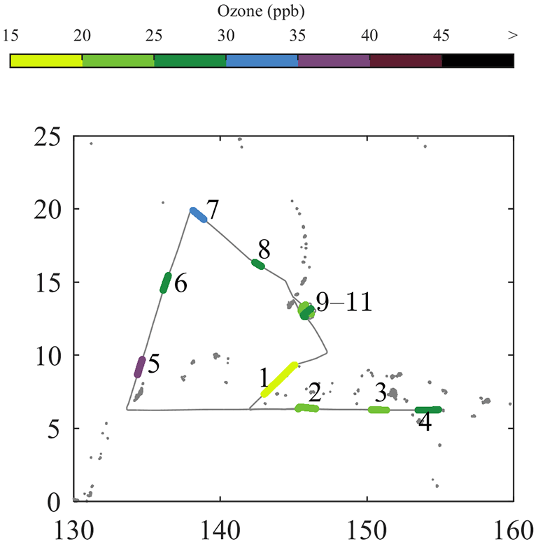
Figure 18Flight track of RF04 with each profile coloured by mean tropospheric ozone as in Fig. 12.
Evidence of an interhemispheric difference in boundary-layer ozone at the time of year of the CAST/CONTRAST/ATTREX campaigns may be found in measurements made by the HIPPO (HIAPER Pole-to-Pole Observations) programme (Wofsy, 2011), which measured latitudinal transects of a range of trace gases along the International Date Line and over the warm pool (see http://hippo.ucar.edu/instruments/chemistry.html). For HIPPO-1, in January 2009, and HIPPO-3, in March–April 2010 (the two missions closest in time of year to the ATTREX campaign), boundary-layer ozone concentrations below 15 ppbv were found between 5∘ N and 20∘ S. In addition, profiles near 15∘ S in January and 2∘ S in March–April showed values < 15 ppbv extending up to 5 km. By contrast, ozone concentrations in January were > 15 ppbv north of 5∘ N in the boundary layer and > 20 ppbv north of 5∘ S above 2 km, while in March–April they exceeded 20 ppbv at all altitudes north of 1∘ N. It is therefore likely that the differences measured in the TTL in ATTREX originated from the interhemispheric differences in boundary-layer ozone concentrations.
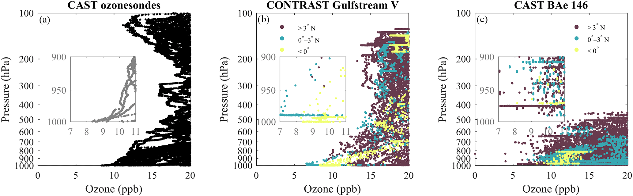
Figure 19Complete dataset of ozone measurements from the CAST ozonesondes (a), the CONTRAST Gulfstream V aircraft (b) and the CAST FAAM BAe 146 aircraft (c), with the aircraft data split into the Southern Hemisphere measurements (yellow), Equator–3∘ N (blue) and higher Northern Hemisphere latitudes (purple). In all cases, minimum ozone near the surface was lower than minimum ozone in the mid-troposphere. The insets show the low ozone concentrations measured in the lowest 100 hPa of the atmosphere in each case.
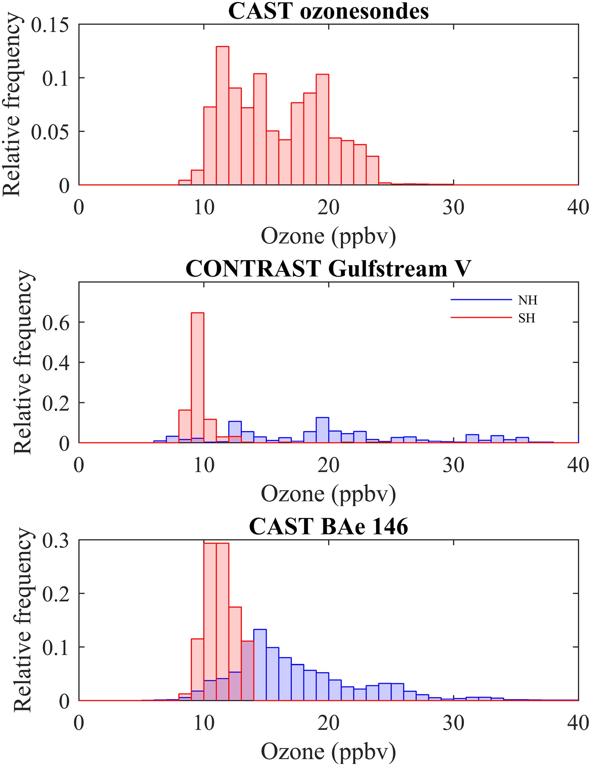
Figure 20Histograms of ozone concentrations in the lowest 100 hPa from CAST ozonesondes, CONTRAST Gulfstream V and the CAST FAAM BAe 146 aircraft, split into Northern Hemisphere data (blue) and Southern Hemisphere data (red).
The ozonesonde and Global Hawk measurements found TTL concentrations below 15 ppbv only in the Southern Hemisphere, but the sparse sampling means that similar layers in the Northern Hemisphere may just have been missed. Many more flights of the CAST and CONTRAST aircraft were made during February 2014, extending from sea level to 120 hPa. We now examine the measurements from these aircraft for evidence of very low ozone concentrations.
The FAAM BAe 146 aircraft focused on measuring close to the surface and within the boundary layer, making 25 flights between 18 January and 18 February (Harris et al., 2017). The NCAR Gulfstream V mostly measured in the upper troposphere in the region of main convective outflow, although many measurements were also made in the boundary layer (Pan et al., 2017); it conducted 13 research flights and three transit flights between 11 January and 28 February.
Other than the brief excursion to 1∘ S on 4 February, the FAAM aircraft flew exclusively in the Northern Hemisphere, as its range was insufficient to reach the Southern Hemisphere from Guam. The NCAR Gulfstream V crossed into the Southern Hemisphere on only two occasions; thus, its measurements also are predominantly in the Northern Hemisphere.
The ozone data from the two aircraft and the CAST ozonesondes from Manus Island (see Sect. 3) are summarized in Fig. 19. In all three panels, ozone concentrations below 15 ppbv are frequently found below 700 hPa. The ozonesondes show a second region of ozone-poor air in the TTL, corresponding to the event discussed in Sect. 3, but the CONTRAST data do not – there are isolated examples around 15 ppbv up to ∼ 180 hPa but not above. Then FAAM aircraft's ceiling is around 300 hPa so it did not measure in the TTL, but again there are only a few ozone values lower than 15 ppbv above 700 hPa. The histograms of the boundary-layer measurements by the CAST ozonesondes and the CAST and CONTRAST aircraft (Fig. 20) show the majority of the measurements in the Southern Hemisphere were below 15 ppbv, whereas the Northern Hemisphere measurements were broadly distributed with a large proportion of measurements above 20 ppbv.
These results are consistent with a hemispheric difference in the ozone distribution in the boundary layer over the warm pool, which resulted in the layers of very low ozone concentrations being lifted to the TTL around the Equator and further south but not in the Northern Hemisphere.

Figure 21Panel plot of six compounds measured by the whole air samplers aboard the three aircraft. The red line indicates the average profile of measurements taken where ozone was above 20 ppbv, and the blue line is the average profile for ozone below 20 ppbv.
WASs aboard the CAST, CONTRAST and ATTREX aircraft provided measurements of very short-lived substances (VSLSs), of which eight were measured by all three aircraft: dimethyl sulfide ((CH3)2S), iodomethane (CH3I), tribromomethane (CHBr3), dibromochloromethane (CHBr2Cl), bromochloromethane (CH2BrCl), dichloromethane (CH2Cl2), dibromomethane (CH2Br2) and trichloromethane (CHCl3).
We present six of these molecules here: dichloromethane and trichloromethane, as well as the species measured by the CONTRAST and ATTREX aircraft but not the CAST aircraft are plotted in the Supplement. Dichloromethane is a predominantly industrially produced chemical with a strong anthropogenic signal and relatively long lifetime (∼ 6 months), while trichloromethane has mostly natural, but some anthropogenic, sources (McCulloch, 2002) and has a long lifetime of ∼ 6 months.
Of the six remaining molecules, the atmospheric lifetimes range from a few minutes to a few months: (CH3)2S has a lifetime between 11 min and 46 h (Marandino et al., 2013); CH3I has a lifetime of ∼ 4 days and CHBr3 a lifetime of ∼ 15 days (Carpenter et al., 2014); that of CHBr2Cl is about 3 months, while CH2Br2 and CH2BrCl have lifetimes of the order of 6 months (Montzka et al., 2010; Mellouki et al., 1992; Leedham Elvidge et al., 2015; Khalil and Rasmussen, 1999).
All six compounds have significant marine sources. (CH3)2S, CHBr3 and CH2Br2 are produced by phytoplankton (Dacey and Wakeham, 1986; Quack et al., 2007; Stemmler et al., 2015). CH3I is produced by cyanobacteria and picoplankton (Smythe-Wright et al., 2006), and large concentrations of CH3I are present in the marine boundary layer (Maloney et al., 2001). CHBr2Cl is produced naturally by various marine macroalgae (Gschwend et al., 1985), and CH2BrCl is emitted by tropical seaweed (Mithoo-Singh et al., 2017).
The vertical profiles obtained from combining all of the whole air sampler data from the entire CAST, CONTRAST and ATTREX campaigns yield the plots in Fig. 21. (The Supplement contains similar plots split into the individual aircraft.) Necessarily, the vast majority of these points are from the Northern Hemisphere, away from the very low ozone concentrations described in Sect. 4.3. Each data point is coloured by the ozone concentration measured at the time the WAS bottles were being filled, and average profiles for each compound were obtained for WAS samples with ozone concentrations less than 20 ppbv (in blue) and for WAS samples with ozone concentrations greater than 20 ppbv (in red). The average profiles were generated by binning the data into 20 equally sized bins in logarithmic pressure space between 1000 and 10 hPa, and averaging the data within that bin.
In the cases of (CH3)2S, CH3I, CHBr3, CHBr2Cl and CH2Br2, all show higher concentrations of the molecule in question when ozone concentrations were less than 20 ppbv (low-ozone regime) compared to when ozone concentrations were greater than 20 ppbv (high-ozone regime), which suggests that the more ozone-deficient air has encountered the marine boundary layer – where these molecules were produced – more recently than the more ozone-rich air. Meanwhile, CH2BrCl shows no difference between the low-ozone regime and the high-ozone regime because of its longer lifetime than the other VSLSs measured.
The 33 species that were measured by just the CONTRAST and ATTREX aircraft are plotted in the Supplement. The species that were of a marine origin show the expected enhancements in the low-ozone regime compared to the high-ozone regime, while the species that were of industrial origin show the reverse: enhancements were found in the high-ozone regime instead.
Very few WAS samples were taken in the Southern Hemisphere – only eight were taken by the FAAM BAe 146, 60 by the Global Hawk and 134 by the Gulfstream V, compared to the Northern Hemisphere where 456 FAAM samples, 1373 Gulfstream V samples and 608 Global Hawk samples were taken. As a result, very few WAS samples were taken in areas where ozone concentrations were at their lowest during the campaign, and further investigation of these halomethanes during very low ozone events would be beneficial in future campaigns.
We have presented an extensive dataset of ozone observations from three research aircraft and ozonesondes over the west Pacific warm pool in February–March 2014, with a particular focus on the TTL. The results point to the generation of layers with very low ozone concentration (< 15 ppbv) just below the tropopause due to uplift by deep convection, confirming the conclusion of Newton et al. (2016) based on the ozonesonde data. The lowest values measured in the TTL, around 10–12 ppbv, are very similar to those measured in the boundary layer in the region, consistent with uplift of boundary-layer air up to the tropopause region. This places boundary-layer air above the level of net radiative heating in the TTL and therefore in a position to ascend into the stratosphere in the Brewer–Dobson circulation. Consequently, it provides a route for very short-lived halocarbon species to reach the stratosphere. Evidence from the extensive whole air samplers carried by the three aircraft shows a negative correlation between ozone and species of marine origin, consistent with uplift in convection.
Despite the far more extensive sampling of the Northern Hemisphere than the Southern Hemisphere during the aircraft campaign, very low ozone concentrations in the TTL were only found in the Southern Hemisphere; even in the outflow of Cyclone Faxai, the Global Hawk measured 15 ppbv of ozone, similar to measurements in convective anvils by the Gulfstream V in the Northern Hemisphere. This suggests a hemispheric difference in the TTL ozone distribution, either because of lower boundary-layer ozone concentrations in the Southern Hemisphere or because of differences in the convective uplift. Previous measurement campaigns in this region point to an interhemispheric difference in boundary-layer ozone concentration as being responsible for the corresponding feature in the TTL.
CAST data are publicly available from the Centre for Environmental Data Analysis (CEDA) at http://catalogue.ceda.ac.uk/uuid/565b6bb5a0535b438ad2fae4c852e1b3 (Braesicke et al., 2014).
CONTRAST data are publicly available from the Earth Observation Laboratory (EOL) data archive at http://data.eol.ucar.edu/master_list/?project=CONTRAST (advanced whole air sampler, AWAS: Atlas, 2014a; NO, NO2, O3 in situ chemiluminescence data: Weinheimer, 2015).
ATTREX data are publicly available from the Earth Science Project Office (ESPO) Data Archive at https://espoarchive.nasa.gov/archive/browse/attrex (AWAS: Atlas, 2014b; Meteorological Measurement System (MMS): Bui, 2014; Unmanned Aircraft Systems (UAS) Chromatograph for Atmospheric Trace Species (UCATS): Elkins, 2014).
The supplement related to this article is available online at: https://doi.org/10.5194/acp-18-5157-2018-supplement.
The authors declare that they have no conflict of interest.
We thank the Natural Environment Research Council (NERC) Facility for Airborne Atmospheric Measurements (FAAM) for
the CAST aircraft data and the Centre for Data Archival (CEDA) for
supporting meteorological data. The project was supported by NERC grant NE/J006173/1. Richard Newton is a
NERC-supported research student. We thank an anonymous reviewer for helpful
comments on the original manuscript.
Edited
by: Jianzhong Ma
Reviewed by: two anonymous referees
Atlas, E.: ATTREX Global Hawk AWAS trace gas mixing ratios, Earth Science Project Office (ESPO) Data Archive, available at: https://espoarchive.nasa.gov/archive/browse/attrex/GHawk/AWAS (last access: April 2018), 2014a. a, b
Atlas, E.: NSF/NCAR GV HIAPER Airborne Instrument Solicitation (HAIS) Advanced Whole Air Sampler, Version 1.0, UCAR/NCAR – Earth Observing Laboratory, https://doi.org/10.5065/D6DF6PK9 (last access: April 2018), 2014b. a, b
Andrews, S. J., Carpenter, L. J., Apel, E. C., Atlas, E., Donets, V., Hopkins, J. R., Hornbrook, R. S., Lewis, A. C., Lidster, R. T., Lueb, R., Minaeian, J., Navarro, M., Punjabi, S., Riemer, D., and Schauffler, S.: A comparison of very short lived halocarbon (VSLS) and DMS aircraft measurements in the tropical west Pacific from CAST, ATTREX and CONTRAST, Atmos. Meas. Tech., 9, 5213–5225, https://doi.org/10.5194/amt-9-5213-2016, 2016. a, b
Apel, E. C., Hills, A. J., Lueb, R., Zindel, S., Eisele, S., and Riemer, D. D.: A fast-GC/MS system to measure C2 to C4 carbonyls and methanol aboard aircraft, J. Geophys. Res.-Atmos., 108, 8794, https://doi.org/10.1029/2002JD003199, 2003. a
Ashfold, M. J., Harris, N. R. P., Atlas, E. L., Manning, A. J., and Pyle, J. A.: Transport of short-lived species into the Tropical Tropopause Layer, Atmos. Chem. Phys., 12, 6309–6322, https://doi.org/10.5194/acp-12-6309-2012, 2012. a
Braesicke, P., Harris, N., Pyle, J. A., Robinson, A., and Vaughan, G.: Co-ordinationed Airborne Studies in the Tropics (CAST): in situ airborne, ozonesonde and ground based and atmospheric chemistry measurements, NCAS British Atmospheric Data Centre, available at: http://catalogue.ceda.ac.uk/uuid/565b6bb5a0535b438ad2fae4c852e1b3 (last access: April 2018), 2014. a, b
Browell, E. V., Fenn, M. A., Butler, C. F., Grant, W. B., Ismail, S., Ferrare, R. A., Kooi, S. A., Brackett, V. G., Clayton, M. B., Avery, M. A., Barrick, J. D. W., Fuelberg, H. E., Maloney, J. C., Newell, R. E., Zhu, Y., Mahoney, M. J., Anderson, B. E., Blake, D. R., Brune, W. H., Heikes, B. G., Sachse, G. W., Singh, H. B., and Talbot, R. W.: Large-scale air mass characteristics observed over the remote tropical Pacific Ocean during March–April 1999: Results from PEM-Tropics B field experiment, J. Geophys. Res.-Atmos., 106, 32481–32501, https://doi.org/10.1029/2001JD900001, 2001. a
Bui, T. P.: ATTREX Global Hawk MMS 1 Hz data, Earth Science Project Office (ESPO) Data Archive, available at: https://espoarchive.nasa.gov/archive/browse/attrex/GHawk/MMS-1HZ (last access: April 2018), 2014. a, b
Carpenter, L. J., Reimann, S., Burkholder, J. B., Clerbaux, C., Hall, B. D., Hossaini, R., Laube, J. C., and Yvon-Lewis, S. A.: Update on Ozone-Depleting Substances (ODSs) and Other Gases of Interest to the Montreal Protocol, in: Scientific Assessment of Ozone Depletion: 2014, chap. 1, 1.1–1.101, World Meteorological Association/United Nations Environment Programme, 2014. a
Dacey, J. W. H. and Wakeham, S. G.: Oceanic Dimethylsulfide: Production During Zooplankton Grazing on Phytoplankton, Science, 233, 1314–1316, https://doi.org/10.1126/science.233.4770.1314, 1986. a
Davies, T., Cullen, M. J. P., Malcolm, A. J., Mawson, M. H., Staniforth, A., White, A. A., and Wood, N.: A new dynamical core for the Met Office's global and regional modelling of the atmosphere, Q. J. Roy. Meteor. Soc., 131, 1759–1782, https://doi.org/10.1256/qj.04.101, 2005. a
Elkins, J. W.: ATTREX Global Hawk UCATS Measurements, Earth Science Project Office (ESPO) Data Archive, available at: https://espoarchive.nasa.gov/archive/browse/attrex/GHawk/UCATS-O3 (last access: April 2018), 2014. a, b
Folkins, I., Loewenstein, M., Podolske, J., Oltmans, S. J., and Proffitt, M.: A barrier to vertical mixing at 14 km in the tropics: Evidence from ozonesondes and aircraft measurements, J. Geophys. Res.-Atmos., 104, 22095–22102, https://doi.org/10.1029/1999JD900404, 1999. a
Folkins, I., Braun, C., Thompson, A. M., and Witte, J.: Tropical ozone as an indicator of deep convection, J. Geophys. Res.-Atmos., 107, 4184, https://doi.org/10.1029/2001JD001178, 2002. a
Frey, W., Schofield, R., Hoor, P., Kunkel, D., Ravegnani, F., Ulanovsky, A., Viciani, S., D'Amato, F., and Lane, T. P.: The impact of overshooting deep convection on local transport and mixing in the tropical upper troposphere/lower stratosphere (UTLS), Atmos. Chem. Phys., 15, 6467–6486, https://doi.org/10.5194/acp-15-6467-2015, 2015. a
Fueglistaler, S., Dessler, A. E., Dunkerton, T. J., Folkins, I., Fu, Q., and Mote, P. W.: Tropical tropopause layer, Rev. Geophys., 47, RG1004, https://doi.org/10.1029/2008RG000267, 2009. a, b
Gao, R. S., Ballard, J., Watts, L. A., Thornberry, T. D., Ciciora, S. J., McLaughlin, R. J., and Fahey, D. W.: A compact, fast UV photometer for measurement of ozone from research aircraft, Atmos. Meas. Tech., 5, 2201–2210, https://doi.org/10.5194/amt-5-2201-2012, 2012. a
Gettelman, A. and de Forster, P. M.: A Climatology of the Tropical Tropopause Layer, J. Meteorol. Soc. Jpn., 80, 911–924, https://doi.org/10.2151/jmsj.80.911, 2002. a
Gschwend, P. M., MacFarlane, J. K., and Newman, K. A.: Volatile Halogenated Organic Compounds Released to Seawater from Temperate Marine Macroalgae, Science, 227, 1033–1035, https://doi.org/10.1126/science.227.4690.1033, 1985. a
Harris, N. R. P., Carpenter, L. J., Lee, J. D., Vaughan, G., Filus, M. T., Jones, R. L., OuYang, B., Pyle, J. A., Robinson, A. D., Andrews, S. J., Lewis, A. C., Minaeian, J., Vaughan, A., Dorsey, J. R., Gallagher, M. W., Le Breton, M., Newton, R., Percival, C. J., Ricketts, H. M. A., Bauguitte, S. J.-B., Nott, G. J., Wellpott, A., Ashfold, M. J., Flemming, J., Butler, R., Palmer, P. I., Kaye, P. H., Stopford, C., Chemel, C., Boesch, H., Humpage, N., Vick, A., MacKenzie, A. R., Hyde, R., Angelov, P., Meneguz, E., and Manning, A. J.: Coordinated Airborne Studies in the Tropics (CAST), B. Am. Meteorol. Soc., 1, 145–162, https://doi.org/10.1175/BAMS-D-14-00290.1, 2017. a, b, c, d
Heyes, W. J., Vaughan, G., Allen, G., Volz-Thomas, A., Pätz, H.-W., and Busen, R.: Composition of the TTL over Darwin: local mixing or long-range transport?, Atmos. Chem. Phys., 9, 7725–7736, https://doi.org/10.5194/acp-9-7725-2009, 2009. a, b, c
Highwood, E. J. and Hoskins, B. J.: The tropical tropopause, Q. J. Roy. Meteor. Soc., 124, 1579–1604, https://doi.org/10.1002/qj.49712454911, 1998. a
Holton, J. R., Haynes, P. H., McIntyre, M. E., Douglass, A. R., Rood, R. B., and Pfister, L.: Stratosphere-troposphere exchange, Rev. Geophys., 33, 403–439, https://doi.org/10.1029/95RG02097, 1995. a
Jensen, E. J., Pfister, L., Jordan, D. E., Thaopaul, V. B., Ueyama, R., Singh, H. B., Thornberry, T. D., Rollins, A. W., Gao, R.-S., Fahey, D. W., Rosenlof, K. H., Elkins, J. W., Diskin, G. S., DiGangi, J. P., Lawson, R. P., Woods, S., Atlas, E. L., Navarro Rodriguez, M. A., Wofsy, S. C., Pittman, J., Bardeen, C. G., Toon, O. B., Kindel, B. C., Newman, P. A., McGill, M. J., Hlavka, D. L., Lait, L. R., Schoeberl, M. R., Bergman, J. W., Selkirk, H. B., Alexander, M. J., Kim, J.-E., Boon, H. L., Stutz, J., and Pfeilsticker, K.: The NASA Airborne Tropical Tropopause Experiment: High-Altitude Aircraft Measurements in the Tropical Western Pacific, B. Am. Meteorol. Soc., 98, 129–143, https://doi.org/10.1175/BAMS-D-14-00263.1, 2017. a, b, c, d
Jones, A., Thomson, D., Hort, M., and Devenish, B.: The U.K. Met Office's Next-Generation Atmospheric Dispersion Model, NAME III, in: Air Pollution Modeling and its Application XVII, edited by: Borrego, C. and Norman, A.-L., Springer US, chap. 62, 580–589, 2007. a
Khalil, M. A. K. and Rasmussen, R. A.: Atmospheric chloroform, Atmos. Environ., 33, 1151–1158, https://doi.org/10.1016/S1352-2310(98)00233-7, 1999. a
Kley, D., Crutzen, P. J., Smit, H. G. J., Vömel, H., Oltmans, S. J., Grassl, H., and Ramanathan, V.: Observations of Near-Zero Ozone Concentrations Over the Convective Pacific: Effects on Air Chemistry, Science, 274, 230–233, https://doi.org/10.1126/science.274.5285.230, 1996. a, b
Kondo, Y., Ko, M., Koike, M., Kawakami, S., and Ogawa, T.: Preface to Special Section on Biomass Burning and Lightning Experiment (BIBLE), J. Geophys. Res.-Atmos., 107, 8397, https://doi.org/10.1029/2002JD002401, 2002a. a
Kondo, Y., Koike, M., Kita, K., Ikeda, H., Takegawa, N., Kawakami, S., Blake, D., Liu, S. C., Ko, M., Miyazaki, Y., Irie, H., Higashi, Y., Liley, B., Nishi, N., Zhao, Y., and Ogawa, T.: Effects of biomass burning, lightning, and convection on O3, CO, and NOy over the tropical Pacific and Australia in August–October 1998 and 1999, J. Geophys. Res.-Atmos., 107, 8402, https://doi.org/10.1029/2001JD000820, 2002b. a
Leedham Elvidge, E. C., Oram, D. E., Laube, J. C., Baker, A. K., Montzka, S. A., Humphrey, S., O'Sullivan, D. A., and Brenninkmeijer, C. A. M.: Increasing concentrations of dichloromethane, CH2Cl2, inferred from CARIBIC air samples collected 1998–2012, Atmos. Chem. Phys., 15, 1939–1958, https://doi.org/10.5194/acp-15-1939-2015, 2015. a
Maloney, J. C., Fuelberg, H. E., Avery, M. A., Crawford, J. H., Blake, D. R., Heikes, B. G., Sachse, G. W., Sandholm, S. T., Singh, H., and Talbot, R. W.: Chemical characteristics of air from different source regions during the second Pacific Exploratory Mission in the Tropics (PEM-Tropics B), J. Geophys. Res.-Atmos., 106, 32609–32625, https://doi.org/10.1029/2001JD900100, 2001. a
Marandino, C. A., Tegtmeier, S., Krüger, K., Zindler, C., Atlas, E. L., Moore, F., and Bange, H. W.: Dimethylsulphide (DMS) emissions from the western Pacific Ocean: a potential marine source for stratospheric sulphur?, Atmos. Chem. Phys., 13, 8427–8437, https://doi.org/10.5194/acp-13-8427-2013, 2013. a
McCulloch, A.: Chloroform in the environment: Occurrence, sources, sinks and effects, EuroChlor, chap. 2, 3–9, 2002. a
Mellouki, A., Talukdar, R. K., Schmoltner, A.-M., Gierczak, T., Mills, M. J., Solomon, S., and Ravishankara, A. R.: Atmospheric lifetimes and ozone depletion potentials of methyl bromide (CH3Br) and dibromomethane (CH2Br2), Geophys. Res. Lett., 19, 2059–2062, https://doi.org/10.1029/92GL01612, 1992. a
Meneguz, E. and Thomson, D. J.: Towards a new scheme for parametrisation of deep convection in NAME III, Int. J. Environ. Pollut., 54, 128–136, https://doi.org/10.1504/IJEP.2014.065113, 2014. a
Mithoo-Singh, P. K., Keng, F. S.-L., Phang, S.-M. Leedham Elvidge, E. C., Sturges, W. T., Malin, G., and Abd Rahman, N.: Halocarbon emissions by selected tropical seaweeds: species-specific and compound-specific responses under changing pH, PeerJ, 5, e2918, https://doi.org/10.7717/peerj.2918, 2017. a
Montzka, S. A., Reimann, S., Engel, A., Krüger, K., O'Doherty, S., and Sturges, W. T.: Ozone-Depleting Substances (ODSs) and Related Chemicals, in: Scientific Assessment of Ozone Depletion: 2010, chap. 1, World Meteorological Association/United Nations Environment Programme, 1.1–1.108, 2010. a
Newton, R., Vaughan, G., Ricketts, H. M. A., Pan, L. L., Weinheimer, A. J., and Chemel, C.: Ozonesonde profiles from the West Pacific Warm Pool: measurements and validation, Atmos. Chem. Phys., 16, 619–634, https://doi.org/10.5194/acp-16-619-2016, 2016. a, b, c, d, e, f, g, h, i
Oltmans, S. J., Johnson, B. J., Harris, J. M., Vömel, H., Thompson, A. M., Koshy, K., Simon, P., Bendura, R. J., Logan, J. A., Haseba, F., Shiotani, M., Kirchhoff, V. W. J. H., Maata, M., Sami, G., Samad, A., Tabuadravu, J., Enriquez, H., Agama, M., Cornejo, J., and Paredes, F.: Ozone in the Pacific tropical troposphere from ozonesonde observations, J. Geophys. Res.-Atmos., 106, 32503–32525, https://doi.org/10.1029/2000JD900834, 2001. a
Pan, L. L., Honomichl, S. B., Randel, W. J., Apel, E. C., Atlas, E. L., Beaton, S. P., Bresch, J. F., Hornbrook, R., Kinnison, D. E., Lamarque, J.-F., Saiz-Lopez, A., Salawitch, R. J., and Weinheimer, A. J.: Bimodal distribution of free tropospheric ozone over the tropical western Pacific revealed by airborne observations, Geophys. Res. Lett., 42, 7844–7851, https://doi.org/10.1002/2015GL065562, 2015. a
Pan, L. L., Atlas, E. L., Salawitch, R. J., Honomichl, S. B., Bresch, J. F., Randel, W. J., Apel, E. C., Hornbrook, R. S., Weinheimer, A. J., Anderson, D. C., Andrews, S. J., Baidar, S., Beaton, S. P., Campos, T. L., Carpenter, L. J., Chen, D., Dix, B., Donets, V., Hall, S. R., Hanisco, T. F., Homeyer, C. R., Huey, L. G., Jensen, J. B., Kaser, L., Kinnison, D. E., Koenig, T. K., Lamarque, J.-F., Liu, C., Luo, J., Luo, Z. J., Montzka, D. D., Nicely, J. M., Pierce, R. B., Riemer, D. D., Robinson, T., Romashkin, P., Saiz-Lopez, A., Schauffler, S., Shieh, O., Stell, M. H., Ullmann, K., Vaughan, G., Volkamer, R., and Wolfe, G.: The Convective Transport of Active Species in the Tropics (CONTRAST) Experiment, B. Am. Meteorol. Soc., 98, 106–128, https://doi.org/10.1175/BAMS-D-14-00272.1, 2017. a, b, c, d
Petropavlovskikh, I., Ray, E., Davis, S. M., Rosenlof, K., Manney, G., Shetter, R., Hall, S. R., Ullmann, K., Pfister, L., Hair, J., Fenn, M., Avery, M., and Thompson, A. M.: Low-ozone bubbles observed in the tropical tropopause layer during the TC4 campaign in 2007, J. Geophys. Res.-Atmos., 115, D00J16, https://doi.org/10.1029/2009JD012804, 2010. a
Quack, B., Peeken, I., Petrick, G., and Nachtigall, K.: Oceanic distribution and sources of bromoform and dibromomethane in the Mauritanian upwelling, J. Geophys. Res.-Oceans, 112, C10006, https://doi.org/10.1029/2006JC003803, 2007. a
Rex, M., Wohltmann, I., Ridder, T., Lehmann, R., Rosenlof, K., Wennberg, P., Weisenstein, D., Notholt, J., Krüger, K., Mohr, V., and Tegtmeier, S.: A tropical West Pacific OH minimum and implications for stratospheric composition, Atmos. Chem. Phys., 14, 4827–4841, https://doi.org/10.5194/acp-14-4827-2014, 2014. a, b
Ridley, B. A., Grahek, F. E., and Walega, J. G.: A Small High-Sensitivity, Medium-Response Ozone Detector Suitable for Measurements from Light Aircraft, J. Atmos. Ocean. Tech., 9, 142–148, https://doi.org/10.1175/1520-0426(1992)009<0142:ASHSMR>2.0.CO;2, 1992. a
Ryall, D. B., Derwent, R. G., Manning, A. J., Simmonds, P. G., and O'Doherty, S.: Estimating source regions of European emissions of trace gases from observations at Mace Head, Atmos. Environ., 35, 2507–2523, https://doi.org/10.1016/S1352-2310(00)00433-7, 2001. a
Schauffler, S. M., Atlas, E. L., Blake, D. R., Flocke, F., Lueb, R. A., Lee-Taylor, J. M., Stroud, V., and Travnicek, W.: Distributions of brominated organic compounds in the troposphere and lower stratosphere, J. Geophys. Res.-Atmos., 104, 21513–21535, https://doi.org/10.1029/1999JD900197, 1999. a
Singh, H. B., Gregory, G. L., Anderson, B., Browell, E., Sachse, G. W., Davis, D. D., Crawford, J., Bradshaw, J. D., Talbot, R., Blake, D. R., Thornton, D., Newell, R., and Merrill, J.: Low ozone in the marine boundary layer of the tropical Pacific Ocean: Photochemical loss, chlorine atoms, and entrainment, J. Geophys. Res.-Atmos., 101, 1907–1917, https://doi.org/10.1029/95JD01028, 1996. a
Smythe-Wright, D., Boswell, S. M., Breithaupt, P., Davidson, R. D., Dimmer, C. H., and Eiras Diaz, L. B.: Methyl iodide production in the ocean: Implications for climate change, Global Biogeochem. Cy., 20, GB3003, https://doi.org/10.1029/2005GB002642, 2006. a
Stein, A. F., Draxler, R. R., Rolph, G. D., Stunder, B. J. B., Cohen, M. D., and Ngan, F.: NOAA's HYSPLIT Atmospheric Transport and Dispersion Modeling System, B. Am. Meteorol. Soc., 96, 2059–2077, https://doi.org/10.1175/BAMS-D-14-00110.1, 2015. a
Stemmler, I., Hense, I., and Quack, B.: Marine sources of bromoform in the global open ocean – global patterns and emissions, Biogeosciences, 12, 1967–1981, https://doi.org/10.5194/bg-12-1967-2015, 2015. a
Vömel, H. and Diaz, K.: Ozone sonde cell current measurements and implications for observations of near-zero ozone concentrations in the tropical upper troposphere, Atmos. Meas. Tech., 3, 495–505, https://doi.org/10.5194/amt-3-495-2010, 2010. a, b
Weinheimer, A. J.: NSF/NCAR GV HIAPER In Situ Chemiluminescence NO, NO2, O3 Data, Version 3.0, UCAR/NCAR – Earth Observing Laboratory, https://doi.org/10.5065/D6PK0D6N (last access: April 2018), 2015. a, b
Wilks, D. S.: Statistical Methods in the Atmospheric Sciences, 1st edn., chap. 6, p. 127, Academic Press, 1995. a
Wofsy, S. C.: HIAPER Pole-to-Pole Observations (HIPPO): fine-grained, global-scale measurements of climatically important atmospheric gases and aerosols, Philos. T. R. Soc. A, 369, 2073–2086, https://doi.org/10.1098/rsta.2010.0313, 2011. a