the Creative Commons Attribution 4.0 License.
the Creative Commons Attribution 4.0 License.
 | 27 Nov 2018
Aerosol water parameterization: long-term evaluation and importance for climate studies
Swen Metzger
Mohamed Abdelkader
Benedikt Steil
Klaus Klingmüller
We scrutinize the importance of aerosol water for the aerosol optical depth (AOD) calculations using a long-term evaluation of the EQuilibrium Simplified Aerosol Model v4 for climate modeling. EQSAM4clim is based on a single solute coefficient approach that efficiently parameterizes hygroscopic growth, accounting for aerosol water uptake from the deliquescence relative humidity up to supersaturation. EQSAM4clim extends the single solute coefficient approach to treat water uptake of multicomponent mixtures. The gas–aerosol partitioning and the mixed-solution water uptake can be solved analytically, preventing the need for iterations, which is computationally efficient. EQSAM4clim has been implemented in the global chemistry climate model EMAC and compared to ISORROPIA II on climate timescales. Our global modeling results show that (I) our EMAC results of the AOD are comparable to modeling results that have been independently evaluated for the period 2000–2010, (II) the results of various aerosol properties of EQSAM4clim and ISORROPIA II are similar and in agreement with AERONET and EMEP observations for the period 2000–2013, and (III) the underlying assumptions on the aerosol water uptake limitations are important for derived AOD calculations. Sensitivity studies of different levels of chemical aging and associated water uptake show larger effects on AOD calculations for the year 2005 compared to the differences associated with the application of the two gas–liquid–solid partitioning schemes. Overall, our study demonstrates the importance of aerosol water for climate studies.
- Article
(10243 KB) - Full-text XML
-
Supplement
(9977 KB) - BibTeX
- EndNote


Providing realistic projections of climate change is difficult due to many unknowns and large uncertainties that still exist (Intergovernmental Panel on Climate Change, 2014). For instance, the recent study by Klingmueller et al. (2016) suggests that the observed increase in aerosol optical depth (AOD) over large parts of the Middle East during the period 2001–2012 could to some extent prevail as a result of climate change. Even in absence of growing anthropogenic aerosol and aerosol precursor emissions, increasing temperature and decreasing relative humidity (RH), as seen in the last decade, promote soil drying, which can lead to increased dust (DU) emissions and hence AOD. Moreover, the discrepancies in the geographical patterns of AOD and aerosol mass measurements can be conclusively explained by aerosol water mass calculations (Nguyen et al., 2016). In fact, in arid regions the water uptake on DU aerosols also becomes important, if air pollution interacts with DU outbreaks (Abdelkader et al., 2015). The uptake of acids on mineral DU can alter the ability of bulk DU to take up water vapor even at a very low ambient RH – in the case of condensing hydrochloric acid (HCl), calcium chloride (CaCl2) can be formed over time, which can cause water uptake at a RH as low as 28 %. While this might be the case for arid regions all over the Earth, it is not an easy task for climate modelers to correctly quantify the effect due to the complexity of the underlying processes, as indicated by the studies of Abdelkader et al. (2017). To reduce uncertainties, our latter two studies applied the DU emissions scheme of Astitha et al. (2012) together with our chemical speciation of the emissions fluxes (see Sect. 2.4) in order to resolve a chemical aging of mineral DU particles (see Sect. 4.2). Furthermore, an interaction of the emission flux with meteorology (Klingmueller et al., 2018) and anthropogenic pollutants, together with a water-mass-conserving coupling of the aerosol hygroscopic growth into haze and clouds (Metzger and Lelieveld, 2007), is needed.
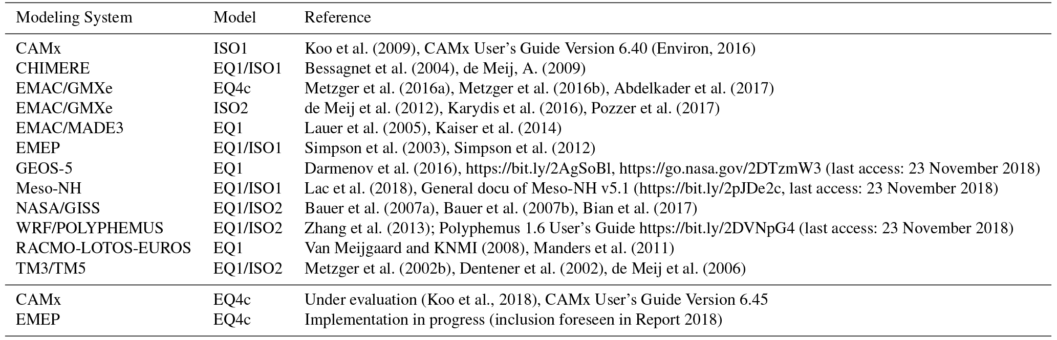
Proper hygroscopic growth calculations require thermodynamic models that can calculate at least the equilibrium partitioning of aerosols and their precursor gases from different natural sources in interaction with anthropogenic air pollution. To calculate the gas–liquid–solid phase partitioning, a variety of thermodynamic equilibrium models have therefore been developed (Metzger et al., 2016a, and references therein). For instance, MARS (Saxena et al., 1986) is widely used in regional modeling as the thermodynamic core of MADE/SORGAM (Ackermann et al., 1998; Schell et al., 2001) through applications of the Weather Research and Forecasting model coupled to Chemistry (WRF-Chem, https://ruc.noaa.gov/wrf/wrf-chem/, last access: 23 November 2018, Ahmadov and Kazil, 2018), the model of the European Monitoring and Evaluation Programme (EMEP, http://www.emep.int/, last access: 23 November 2018 Simpson et al., 2012), and the European Air Pollution Dispersion model system (EURAD, http://www.eurad.uni-koeln.de/, last access: 23 November 2018). Conversely, for climate modeling, mainly ISORROPIA (Fountoukis and Nenes, 2007; Nenes et al., 1998) and EQSAM (Metzger et al., 2002a, 2006) are widely used because of their computational efficiency. Both codes (among others) were recently used for the investigation of global particulate nitrate as part of the Aerosol Comparisons between Observations and Models (AeroCom) phase III experiment (Bian et al., 2017). In addition to this AeroCom study, different EQSAM versions have been used for various other modeling studies, e.g., EQSAM1 (up to EQSAM_v03d): Metzger et al. (2002a, b), Dentener et al. (2002), Lauer et al. (2005), Tsigaridis et al. (2006), Myhre et al. (2006), Luo et al. (2007), Bauer et al. (2007a, b); EQSAM2: Trebs et al. (2005) and Metzger et al. (2006); EQSAM3: Metzger and Lelieveld (2007) and Bruehl et al. (2012). An overview of widely used modeling systems that provide an option to use either EQSAM and/or ISORROPIA is given in Table 1.
Koo et al. (2009)(Environ, 2016)Bessagnet et al. (2004)de Meij, A. (2009)Metzger et al. (2016a)Metzger et al. (2016b)Abdelkader et al. (2017)de Meij et al. (2012)Karydis et al. (2016)Pozzer et al. (2017)Lauer et al. (2005)Kaiser et al. (2014)Simpson et al. (2003)Simpson et al. (2012)Darmenov et al. (2016)Lac et al. (2018)Bauer et al. (2007a)Bauer et al. (2007b)Bian et al. (2017)Zhang et al. (2013)Van Meijgaard and KNMI (2008)Manders et al. (2011)Metzger et al. (2002b)Dentener et al. (2002)de Meij et al. (2006)(Koo et al., 2018)Table 1Modeling systems that provide an option to use EQSAM and/or ISORROPIA. References are given for certain model versions: EQSAM_v03d (EQ1, Metzger et al., 2002a), EQSAM2 (EQ2, Metzger et al., 2006), EQSAM3 (EQ3, Metzger and Lelieveld, 2007), EQSAM4clim (EQ4c, Metzger et al., 2016a) and/or ISORROPIA I (ISO1, Nenes et al., 1998), and ISORROPIA II (ISO2, Fountoukis and Nenes, 2007). URL: CAMx – http://www.camx.com (last access: 23 November 2018); CHIMERE – http://www.lmd.polytechnique.fr/chimere/ (last access: 23 November 2018); EMAC – http://www.messy-interface.org/ (last access: 23 November 2018); EMEP – http://www.emep.int (last access: 23 November 2018); GEOS – https://gmao.gsfc.nasa.gov/GEOS (last access: 23 November 2018); LOTOS-EUROS – https://lotos-euros.tno.nl (last access: 23 November 2018); Meso-NH – http://mesonh.aero.obs-mip.fr/ (last access: 23 November 2018); NASA GISS – https://www.giss.nasa.gov (last access: 23 November 2018); POLYPHEMUS – http://cerea.enpc.fr/polyphemus (last access: 23 November 2018); RACMO – https://www.knmi.nl/ (last access: 23 November 2018); WRF – https://www.mmm.ucar.edu/weather-research-and-forecasting-model (last access: 23 November 2018).
To reduce computational costs, both EQSAM and ISORROPIA follow the MARS approach (Binkowski and Shankar, 1995; Saxena et al., 1986) to determine certain domains by the degree of sulfuric acid neutralization and then divide the RH and composition space into subdomains to minimize the number of equations to be solved. But in contrast to EQSAM, all other thermodynamic equilibrium models require an iterative procedure to solve the ionic composition, which adds significantly to computational costs.
To accurately parameterize the aerosol hygroscopic growth by also considering the Kelvin effect as described by Metzger et al. (2012), the EQSAM approach (Metzger et al., 2002a) was recently extended by Metzger et al. (2016a). The new model version, the EQuilibrium Simplified Aerosol Model v4 for climate modeling, enables aerosol water uptake calculations of concentrated nanometer-sized particles up to dilute solutions, i.e., from the compounds RH of deliquescence (RHD) up to supersaturation (Köhler theory). EQSAM4clim extends the single solute coefficient approach of Metzger et al. (2012) to multicomponent mixtures, including semi-volatile ammonium compounds and major crustal elements. The advantage of EQSAM4clim is that the entire gas–liquid–solid aerosol phase partitioning and water uptake including major mineral cations (Sect. 2.3) can now be solved analytically without iterations, which potentially can significantly speed up computations on climate timescales (Appendix B). Since the thermodynamics of the few widely used equilibrium models such as MARS are limited to either the ammonium–sulfate–nitrate–water system or only include sodium and chloride but no crustal compounds such as calcium, magnesium, and potassium, EQSAM4clim has been evaluated with its introduction against ISORROPIA II at various levels of complexity. It was shown by Metzger et al. (2016a) that the results of EQSAM4clim and ISORROPIA II are similar for reference box-model calculations, textbook examples, and 3-D applications on timescales of individual years.
To scrutinize the importance of aerosol water for climate applications, we evaluate the AOD calculations of EQSAM4clim and ISORROPIA II on climate timescales. For this purpose we extend the model evaluation of Metzger et al. (2016a) by using the comprehensive chemistry–climate and Earth system model EMAC in a setup similar to that applied in our studies on (i) the DU–air pollution dynamics over the eastern Mediterranean (Abdelkader et al., 2015), (ii) the sensitivity of transatlantic DU transport to chemical aging and related atmospheric processes (Abdelkader et al., 2017), and (iii) the comparison of the Metop PMAp2 AOD products using model data (EUMETSAT ITT 15/210839, Final Report, Metzger et al., 2016b). These studies employ a highly complex chemistry setup, particularly with respect to the gas and aqueous phase chemistry and the associated chemical aging of primary aerosols. Since all three studies revealed the importance of chemical aging of primary DU particles for the calculation of the AOD, due to the regional amplification by the aerosol water uptake, it is important to also evaluate the aerosol water parameterization on climate timescales. Our EMAC model setup is described in Sect. 2 and evaluated in Sect. 3 for three periods, 2005, 2000–2010, and 2000–2013, and different model setups that are scrutinized in Sect. 4. Additional results are presented in the Supplement.
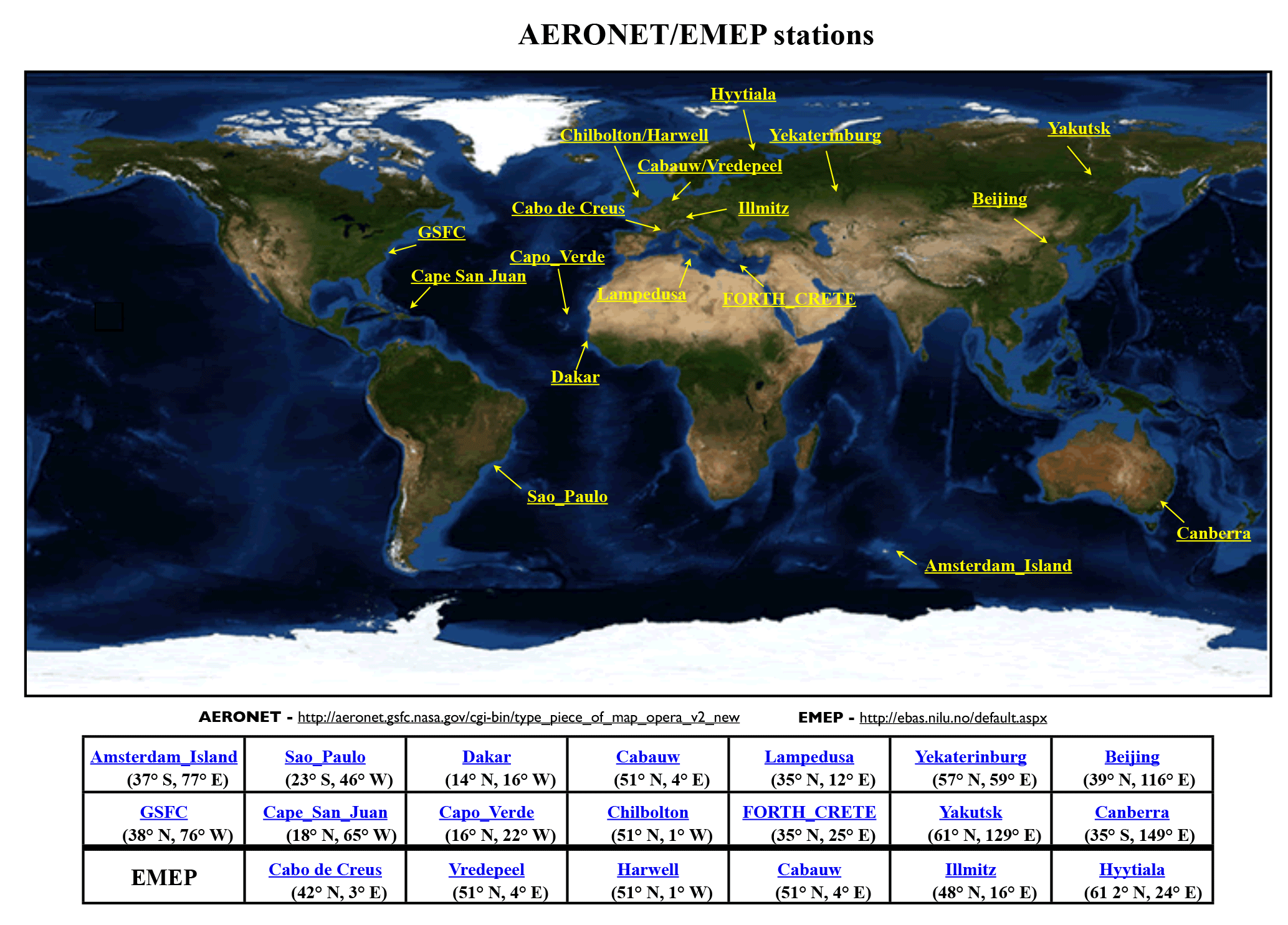
Figure 1Locations of selected AERONET and EMEP stations used in this EMAC evaluation study. The corresponding regions are shown in Fig. S1 (Supplement).
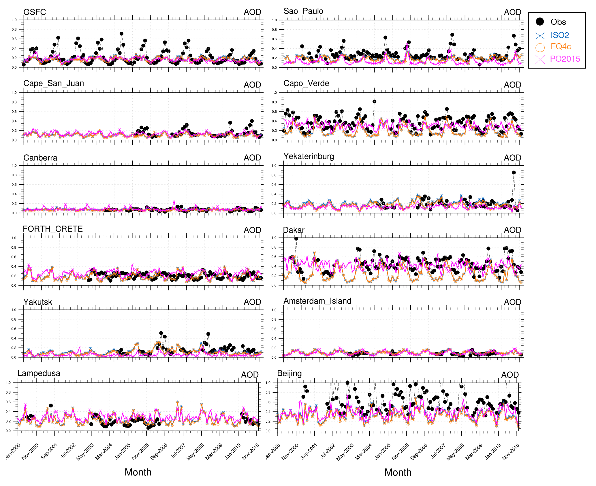
Figure 2Selected AOD time series for 2000–2010 (monthly means) for the stations shown in Fig. 1, representing all regions of Fig. S1. EMAC results based on ISORROPIA II (ISO2), EQSAM4clim (EQ4c) versus AERONET observations (black circles), and Pozzer et al. (2015) (PO2015). Additionally, scatter plots (Figs. S2–S4) are shown in the Supplement for 537 AERONET stations (Fig. S1).
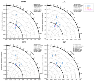
Figure 3Taylor diagram for satellite and model AOD (2000–2010 mean). MODIS (1), MODIS-Aqua (2), MODIS-Deep Blue (3), MISR (4), SeaWIFS (5), ENVISAT (6), and models (7), i.e., ISORROPIA II (ISO2), EQSAM4clim (EQ4c), Pozzer et al. (2015) (PO2015), versus AERONET observations for the four seasons: spring (MAM), summer (JJA), autumn (SON), and winter (DJF). The number of observational points used in the seasonal analysis are shown in parentheses.
2.1 Atmospheric chemistry–climate model EMAC
We use the atmospheric chemistry–climate model EMAC following Abdelkader et al. (2015). EMAC comprises a numerical chemistry and climate simulation system that includes sub-models describing tropospheric and middle atmosphere processes and their interaction with oceans, land, and human influences (Joeckel et al., 2005, 2006a, b, 2008, 2010, 2016). The core atmospheric model, i.e., the fifth-generation European Centre Hamburg general circulation model (ECHAM5, Röckner et al., 2006), is applied with a spherical truncation of T42 and T106 (Gaussian grid of and in latitude and longitude) and 31 vertical hybrid pressure levels up to 10 hPa. Our model setup comprises several sub-models that are described below (for details see http://www.messy-interface.org/, last access: 23 November 2018).
Dry deposition (DDEP) and sedimentation (SEDI) are described by Kerkweg et al. (2006a) and are based on the big leaf approach. Deposition fluxes are calculated as the product of the surface layer concentration and the dry deposition velocity, which reflects the efficiency of the transport to and destruction at the surface (Ganzeveld et al., 2006). Wet deposition (SCAV) is described by Tost et al. (2006a), while its impact on atmospheric composition is detailed by Tost et al. (2006b) and Tost et al. (2007). The offline (OFFEMIS) and online (ONEMIS) emission calculations, including tracer nudging (TNUDGE), are described by Kerkweg et al. (2006b), while the sea–air exchange submodel (AIRSEA) calculates the transfer velocity for certain soluble tracers (e.g., methanol, acetone, propane, propene, CO2, and dimethylsulfide, DMS) (Pozzer et al., 2006). The atmospheric chemistry is calculated with the chemistry submodel (MECCA), which was introduced with Sander et al. (2005).
Our chemical mechanism for the troposphere is similar to the one used in Pozzer et al. (2012) – initially described in Joeckel et al. (2006a) (see their electronic supplement) – although we use a reduced chemistry setup, which consists only of 40 (instead 104) gas phase species and of only 80 (instead 245) chemical reactions. O3-related chemistry of the troposphere is included, but we exclude decomposition of non-methane hydrocarbons (NMHCs) (von Kuhlmann et al., 2003). The other sub-models used in this study are CONVECT (Tost et al., 2006b), and LNOX (Tost et al., 2007) as well as CLOUD, CLOUDOPT, CVTRANS, GWAVE, H2O, JVAL, ORBIT, RAD, SURFACE, and TROPOP (Joeckel et al., 2010). The aerosol radiative properties (AEROPT) (Klingmueller et al., 2014; Pozzer et al., 2012) are based on the scheme by Lauer et al. (2007). AEROPT take the width and mean radii of the lognormal modes into account and consider the composition to obtain the extinction coefficients (σsw,lw), single scattering albedo (ωsw,lw), and asymmetry factors (γsw,lw) for the shortwave (sw) and longwave (lw) radiation. The radiative forcing is fully coupled in our EMAC version with the primary and secondary aerosols obtained with the GMXe aerosol submodel (Sect. 2.2), which includes the associated water mass thermodynamics (Sect. 2.3), whereby the emission fluxes of primary particles are calculated online in feedback with the EMAC model meteorology (Sect. 2.4).
To represent the actual day-to-day meteorology in the troposphere, the model dynamics are weakly nudged (Jeuken et al., 1996; Joeckel et al., 2006a; Lelieveld et al., 2007) towards the analysis data of the European Centre for Medium-Range Weather Forecasts (ECMWF) operational model data (up to 100 hPa). This allows a direct comparison of our model chemistry with ground station and satellite observations (Sect. 3), by using the anthropogenic emission inventory EDGAR Climate Change and Impact Research (CIRCE) (Doering et al., 2009a, b, c) on a high spatial (0.1 by 0.1∘) and moderate temporal (monthly) resolution – see Pozzer et al. (2012) and Pozzer et al. (2017), for example, for details.
2.2 Aerosol microphysics
Aerosol microphysics and the underlying gas–liquid–solid aerosol partitioning is calculated with the Global Modal-aerosol eXtension (GMXe) module, which was described by Pringle et al. (2010a) and Pringle et al. (2010b) but originally developed as part of Metzger and Lelieveld (2007). With GMXe we resolve the aerosol size distribution in seven, i.e., four soluble (nucleation, Aitken, accumulation, and coarse) and three insoluble (Aitken, accumulation, and coarse), log-normal modes. Primary particles are emitted in the insoluble modes (Aitken, accumulation, coarse) and only transferred upon chemical aging and transport to the respective soluble modes (Aitken, accumulation, coarse). Our description of aging depends on the amounts of available condensable compounds that are the outcome of various emission processes (OFFEMIS, ONEMIS) and chemistry calculations (GMXe, MECCA, SCAV). For the chemical aging of bulk species we follow our approach introduced with Abdelkader et al. (2015), which is discussed in Sect. 4.2. The condensation dynamics are calculated within GMXe such that coagulation and hygroscopic growth can alter the aerosol the size distributions. Small particles are efficiently transferred to larger sizes, whereby hygroscopic growth of individual aerosol compounds is calculated from aerosol thermodynamics (Sect. 2.3) based on a chemical speciation of the aerosol emission fluxes (Sect. 2.4). Water uptake of bulk particles (OC, BC, SS, DU), which can be optionally considered, is only treated for aged particles in the soluble modes (Sect. 2.5). Additionally, our EMAC version allows us to consider the aerosol hysteresis effect (Sect. 2.6). To avoid an overlap with cloud formation (especially optical thin clouds) the availability of water vapor is dynamically determined within GMXe. This limits the aerosol hygroscopic growth calculation by either ISORROPIA II or EQSAM4clim, described in Sect. 2.3. Through this specific dynamical coupling, our overall water uptake process depends on meteorology and strongly alters with altitude, independently of the aerosol composition.
2.3 Aerosol thermodynamics
Aerosol thermodynamics is represented by EQSAM4clim (Metzger et al., 2016a) and ISORROPIA II (Fountoukis and Nenes, 2007). Both gas–aerosol partitioning routines calculate the gas–liquid–solid partitioning and aerosol hygroscopic growth. They are embedded in GMXe in exactly the same way, so that a direct comparison of the EMAC modeling results can be made. Deviations can be fully explained by differences in the EQSAM4clim and ISORROPIA II composition calculation approach. Both, EQSAM4clim and ISORROPIA II offer a computationally efficient treatment of the multicomponent and multiphase gas–liquid–solid aerosol partitioning at regional and global scales, by dividing the RH and composition space into subdomains that minimize the number of equations to be solved. However, the EQSAM4clim framework is based on a single solute specific coefficient (vi), which was introduced by Metzger et al. (2012) to efficiently parameterize the water uptake of concentrated nanometer-sized particles up to dilute solutions. In contrast to ISORROPIA II, EQSAM4clim covers the mixed-solution hygroscopic growth considering the Kelvin effect, i.e., water uptake from the compound's RHD up to supersaturation (Köhler theory). It was shown by Metzger et al. (2016a) that the νi approach allows us to analytically solve the gas–liquid–solid partitioning and the mixed-solution water uptake by eliminating the need for numerical iterations, which can significantly speed up our EMAC computations (Appendix B). For a consistent model intercomparison, in this study we limit the gas–aerosol partitioning and associated hygroscopic growth of our EMAC simulations to the inorganic compounds considered by ISORROPIA II. Inorganic aerosol components and their thermodynamic properties used in this study are defined in Table 1 of Metzger et al. (2016a) (with their setup limited already to match the compounds of ISORROPIA II). Thus, we consider the gas–liquid–solid aerosol partitioning and water uptake of the precursor gases water vapor (H2O), sulfuric acid (H2SO4), nitric acid (HNO3), hydrochloric acid (HCl), and ammonia (NH3), together with the major cations sodium (Na+), potassium (K+), calcium (Ca2+), magnesium (Mg2+), and ammonium () and the major anions sulfate (), bisulfate (), nitrate (), and chloride (Cl−), such that nitrate, for example, can replace chloride in sea salt (SS) aerosols (inline with our EQSAM concept described in Metzger et al., 2002a, b, 2006, 2012, 2016a, b; Metzger and Lelieveld, 2007). To enable the full complexity of the phase partitioning with EQSAM4clim and ISORROPIA II, we extend the default EMAC setup through ions assigned to the emission fluxes of primary aerosol particles.
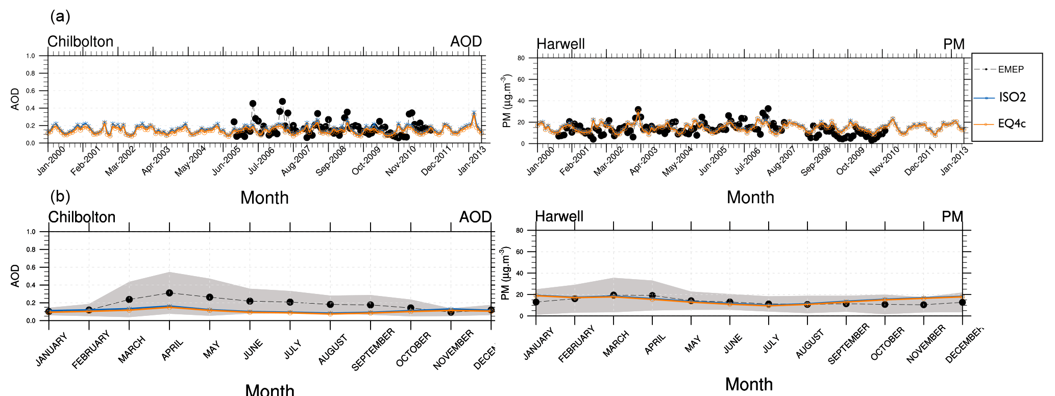
Figure 4AOD and PM time series for 2000–2013 (monthly means): ISORROPIA II (ISO2) and EQSAM4clim (EQ4c) versus AERONET and EMEP observations (a). Panel (b) shows the corresponding climatological year for the AOD and PM (14-year average). The two stations Harwell and Chilbolton (United Kingdom) lie well within one model grid box (51∘ N, 1∘ W).
To calculate the aerosol water uptake of bulk species (see Sect. 2.5), we use Eq. (A3) of Metzger et al. (2016a). Note that Eq. (A3) is an inversion of Eq. (5a) of Metzger et al. (2012), which can be reproduced with the parameters given in Table 2 (with Ke = 1, A = 1, B = 0). As detailed in Sect. 2.7 of Metzger et al. (2016a), the mixed-solution aerosol water uptake can be obtained by their Eq. (22), from tabulated single solute molalities, or parameterized based on Eq. (5a) of Metzger et al. (2012) (Appendix A2, Eq. A3) in agreement with other approaches, including kappa hygroscopicity parameters (see Figs. 3 and 4 of Metzger et al., 2016a, for example). The effect of the implicit assumption (Ke = 1, A = 1, B = 0) on the overall bulk water uptake is negligible for our sensitivity simulations presented in Sect. 4 (studied but not shown).
Table 2Parameters for the different chemical aging levels of bulk species shown in Table 4 (Sect. 4.2). νbulk (−) denotes the bulk water uptake coefficient, RHDbulk (%) the bulk water uptake threshold, and MFbulk (%) the mass fraction used for chemical aging of the bulk aerosol species. The main reagent that is assumed to determine the chemical aging (through implicit coating and water uptake) is included below the bulk species. The values have been empirically determined by numerous model applications and a very comprehensive model evaluation by the constraint to yield the best agreement of our EMAC version with independent model results and various observations. Key results of this evaluation cycle are shown in Sect. 3; additional results will be presented separately.

2.4 Chemical speciation of aerosol emission fluxes
We extend our EMAC setup to include a basic chemical speciation of the natural aerosol emission fluxes in terms of certain cations and/or anions. Usually, climate models treat only bulk tracers such as SS, DU, organic carbon (OC), and black carbon (BC). Instead, we assign ions to the bulk emission fluxes of primary aerosols by using the major cations Na+, K+, Ca2+, and Mg2+ and anions and Cl−. Our concept of chemical speciation was originally developed as part of GMXe by Metzger and Lelieveld (2007) to extend the aerosol water uptake calculations to the so-far chemically unresolved bulk aerosol mass. Thus, for biomass burning OC and BC aerosols, we consider the potassium cation (K+) to be a key reagent (proxy) for the water uptake thermodynamics (Sect. 2.3). For DU, we respectively consider the calcium cation (Ca2+) to be a chemical aging proxy, while we resolve the SS emission fluxes in terms of the seawater composition, considering the major cations Na+, K+, Ca2+, and Mg2+ and anions Cl− and . Our emission fluxes of primary SS and DU particles are calculated online, in feedback with the EMAC meteorology and radiation computations. SS is emitted in two soluble modes (accumulation and coarse) based on the flux parameterization of Monahan et al. (1986), while mineral DU particles are emitted in two insoluble modes (accumulation and coarse), following Astitha et al. (2012). The required parameters for OC, BC, SS and DU used in our sensitivity study (Sect. 4) to scrutinize the bulk water uptake are given in Table 2 and described in Sect. 2.5. Note that Table 2 gives the fraction of DU, for example, that is treated as Ca(Cl)2 for the 50 % (or as Ca(NO3)2 for the 90 %) aging case, though it is relevant only for bulk water uptake calculations. The same is true for SS, OC, and BC. But this DU fraction is not chemically resolved and transported as Ca(Cl)2, so the overall aerosol composition remains unchanged. This is in contrast to our normal (default) GMXe aging, which is considered in all simulations (Sect. 2.2). Within GMXe, the composition of bulk DU and SS is tracked, but the fraction of chemical speciation for the bulk water uptake is prescribed (Table 2). The actual composition is calculated online (Sect. 2.5).
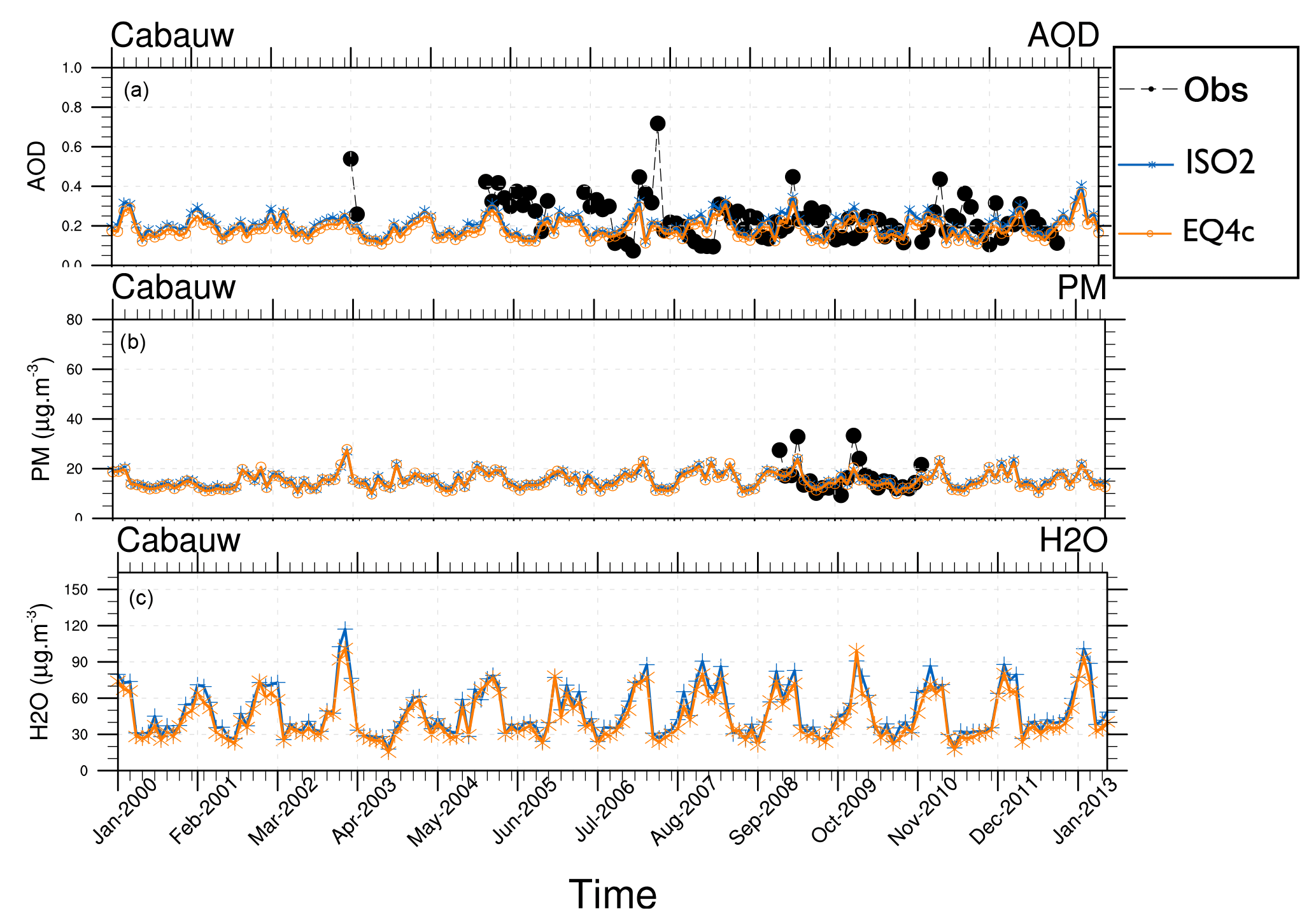
Figure 5AOD (a), total (liquids and solids) particulate matter (PM) (b), and aerosol associated water (c) at EMEP station Cabauw for 2000–2013 (monthly means): ISORROPIA II (ISO2), EQSAM4clim (EQ4c), and AERONET observations (black circles). Available observations are shown. Additionally, various size-resolved aerosol properties are shown in the Supplement (Fig. S5).
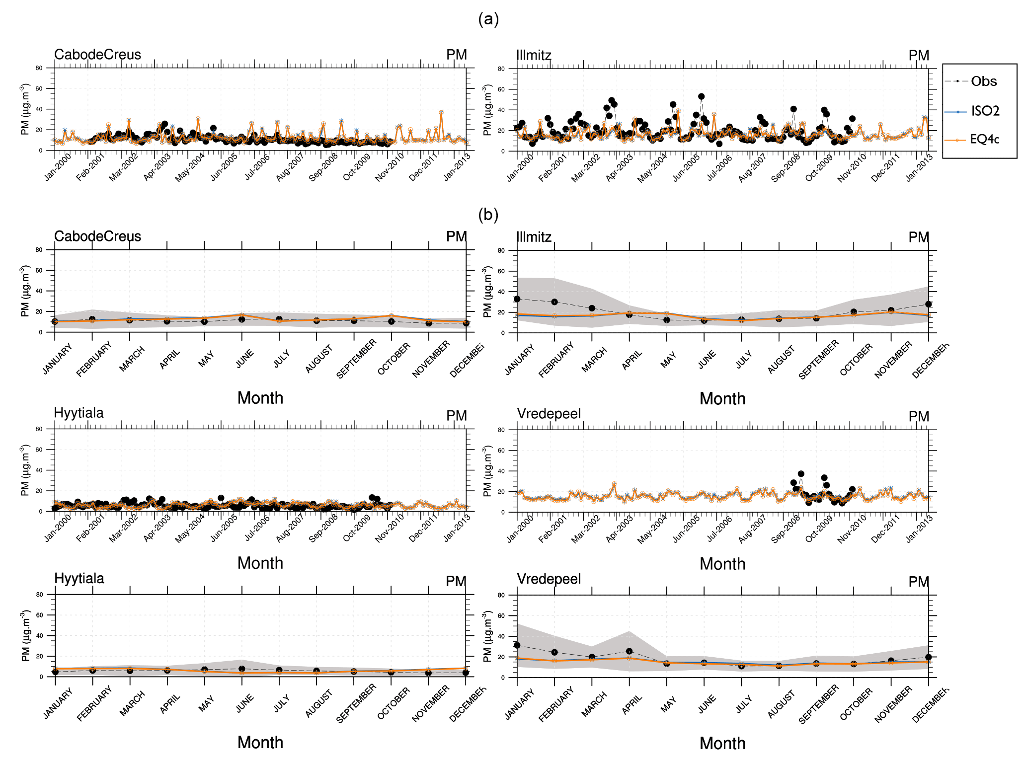
Figure 6Aerosol mass (PM) time series for 2000–2013 (monthly means): ISORROPIA II (ISO2) and EQSAM4clim (EQ4c) versus EMEP stations, which have long-term observations (a). The corresponding climatological year (14-year average) is shown below each time series.
The chemical speciation approach applied in this study was introduced by Abdelkader et al. (2015) and first applied in Abdelkader et al. (2017). As noted in the former publication (p. 9176, line 13–16), our chemical speciation has been determined such that the model concentrations best match the available EMEP and CASTNET measurement data for the period 2000–2013 (to be published separately). Publication of the comprehensive model evaluation is foreseen and in progress.
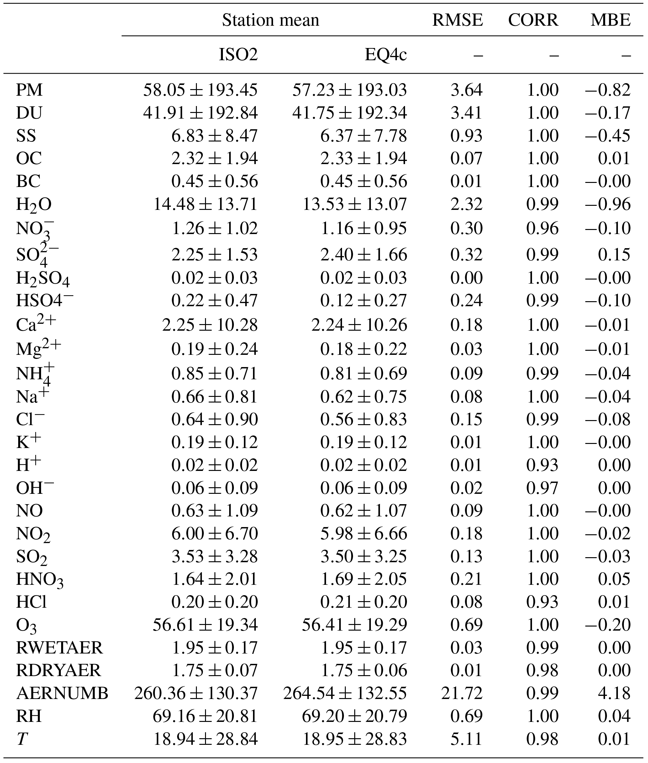
Table 3EMAC tracer statistics for the year 2005 and 189 stations based on 5-hourly model output. Simulations based on ISORROPIA II (ISO2) and EQSAM4clim (EQ4c) (identical EMAC setup).
2.5 Chemical aging and water uptake of bulk aerosols
Our chemical speciation of the primary aerosol emission fluxes is coupled to a chemical aging of bulk species through which salt compounds and associated water can be formed. In our model, the uptake of inorganic acids on bulk compounds and the associated neutralization reactions and water uptake occur during aerosol transport and thus change the (bulk) particle hygroscopicity with time. The chemical aging process is hereby based on explicit neutralization reactions of ions (cations, or anions), which are assigned to the emission fluxes (e.g., K+, Ca2+; see Sect. 2.4). Through the reactions of these cations (anions) with aerosol precursor gases, i.e., major oxidation products of natural and anthropogenic air pollution (here H2SO4, HNO3, HCl, NH3, and H2O), various neutralization (salt) compounds can be formed, e.g., potassium sulfate (K2SO4), potassium bisulfate (KHSO4), potassium nitrate (KNO3), potassium chloride (KCl), calcium sulfate (CaSO4), calcium nitrate (Ca(NO3)2), calcium chloride (CaCl2), and so on for ammonium, sodium, and magnesium; see Table 1 of Metzger et al. (2016a). The salts can cause an uptake of water vapor (H2O) at different ambient humidities, with CaCl2 at RHs as low as 28 %. All salt solutions are subject to the RH and temperature-dependent gas–liquid–solid partitioning as described in Sect. 2.3 and 2.6. For H2O and each cation and anion, a chemical tracer is assigned such that they undergo all aerosol microphysics and thermodynamic processes for their respective GMXe aerosol mode(s) (Sect. 2.2). Through this tracer coupling, each salt compound can alter the subsequent AOD calculations in our EMAC version, most noticeably through an associated aerosol water uptake.
Table 4Sensitivity runs with different levels of chemical aging of bulk species as defined in Sect. 4.2 and Table 2. Note that the key difference between no aging and aging is the water uptake of primary particles. This is only considered for the latter case (being based on Sect. 2.4 and 2.5). All cases include the GMXe coating processes (Sect. 2.2) through condensation of gases such as hydrochloric acid, nitric acid, sulfuric acid, and ammonia on insoluble particles (mineral DU, black, and organic carbon). Additionally, in all cases particles can mix through coagulation, and the formation of semi-volatile salt compounds such as ammonium nitrate and ammonium chloride. Also, the associated gas–aerosol partitioning and water uptake (Sect. 2.3) are always applied for compounds in the soluble modes.

For the chemical aging of our bulk aerosol species (OC, BC, SS, and DU), we assume that bulk OC behaves in terms of water uptake such that it would be coated by ammonium sulfate with a mass fraction of 50 % OC, with the water uptake parameters given in the first sub-column of Table 2. For the 90 % case, ammonium bisulfate is assumed with the water uptake parameters given in the second sub-column (see further explanation in Table 2). To calculate the bulk water uptake, we use the EQSAM4clim parameterizations (introduced by Metzger et al., 2012) and solve a bulk solute molality using Eq. (A3) of Metzger et al. (2016a). For the sake of simplicity, we neglect the Kelvin term (Ke=1, A=1, B=0) and further assume that the water uptake of the bulk compounds can be described by a mean value, for which we can use our single coefficient νi. We further assume a single chemical reagent to be representative for the bulk water uptake due to chemical aging of the bulk aerosol mass, but we only calculate bulk water uptake if the RH exceeds a certain threshold. This aging proxy is given in Table 2 together with the required parameters for our aging setup used in Sect. 4.2. For instance, for the 50 % aging case of bulk SS mass, we assume 50 % of the mass to be subject to water uptake if the RH exceeds a threshold of 50 %. And for this case we assume NaCl as the proxy with νi=1.358 (Table 1 of Metzger et al., 2016a). Accordingly, we assume for DU that 75 % of the mass is subject to water uptake if the RH exceeds the threshold of 28 %, due to a predominant coating by CaCl2 (with νi=2.025).
Table 5CPU times. EMAC @ 96 CPU cores, Cy-Tera (http://web.cytera.cyi.ac.cy/, last access: 23 November 2018).
To distinguish between our EMAC setup that considers the water uptake of normally chemically unresolved particles (SS, DU, OC, BC), in our study we use the label “aging”, referring to a chemical aging that is used in Sect. 4.2. In contrast, our EMAC setup that omits the chemical aging and associated water uptake of bulk aerosols is labeled “no aging” (Sect. 4.1).
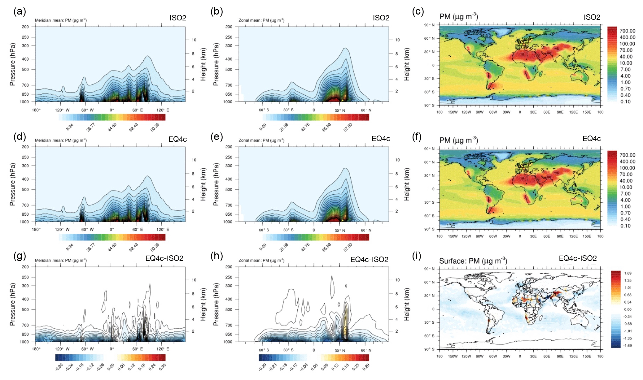
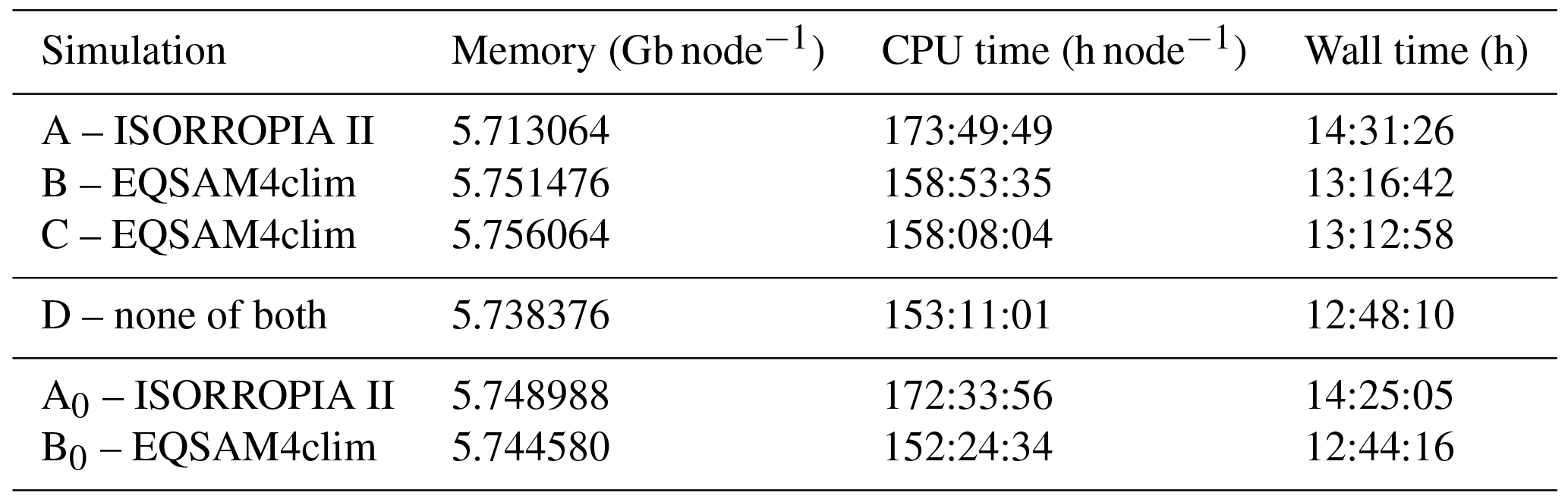
Figure 7Global aerosol distributions of the total (liquids and solids) particulate matter: meridional mean (a, d, g), zonal mean (b, e, h), and atmospheric burden (c, f, i). The EMAC results shown are based on ISORROPIA II (ISO2, a, b, c), EQSAM4clim (EQ4c, d, e, f), and the corresponding difference between both simulations (EQ4c minus ISO2, g, h, i).
Figure 8Figure 7 continued for EMAC aerosol-associated water (2000–2013 mean). Please note the inversion of the color scale (compared to Fig. 7).
Independent of this aging label, all our EMAC simulations consider a comprehensive treatment of the chemical aging of the non-bulk aerosol emission fluxes such that particles can deliquesce or effloresce with age, which is part of our GMXe aerosol dynamical and thermodynamical treatment (Sect. 2.2). The chemical aging includes the dynamically limited condensation of aerosol precursor gases on primary aerosol particles. Our primary aerosol particles are emitted in the insoluble modes and, depending on the coating level (i.e., the amount of gases condensed on the insoluble particles), they are transferred to the soluble modes. But only the chemically identified compounds of the soluble modes (Aitken, accumulation, and coarse mode) are subject to the water uptake calculations by either EQSAM4clim or ISORROPIA II by our no aging setup. Since the inorganic aerosol composition usually explains only a fraction of the emission fluxes, and since the coating process may involve complicated and largely unknown chemical reactions that alter (age) the aerosol surfaces, for our sensitivity study in Sect. 4 we consider the water uptake of the bulk aerosol mass (as described above). Normally, the bulk aerosol mass would be otherwise considered to be dry only. And it was shown by our recent studies by Abdelkader et al. (2015, 2017) and Metzger et al. (2016a, b) that the results of our EMAC aging setup agree better with various ground station observations and satellite measurements.
2.6 Aerosol water mass – hysteresis effect
Our EMAC version further allows us to consider the so-called hysteresis effect. That is, we can obtain the aerosol water mass for two cases, i.e, (1) the dry case, in which RH increases and exceeds the compound's RHD or mixed-solution RHD (Sect. 2.6 of Metzger et al., 2016a), and (2) the wet case, in which the RH decreases until crystallization (efflorescence) point of the dissolved compound(s) is reached. Below these thresholds no aerosol water is calculated. The hysteresis effect can become regionally important since many inorganic salt compounds, which take up water at a given RHD threshold, do not crystallize at the same threshold. The efflorescence thresholds are often observed to be much lower. Although the hysteresis effect might be less pronounced in ambient observations (simply because the aerosol composition usually changes over time due to transport and chemical reactions), the instantaneous effect on radiation can locally become important.
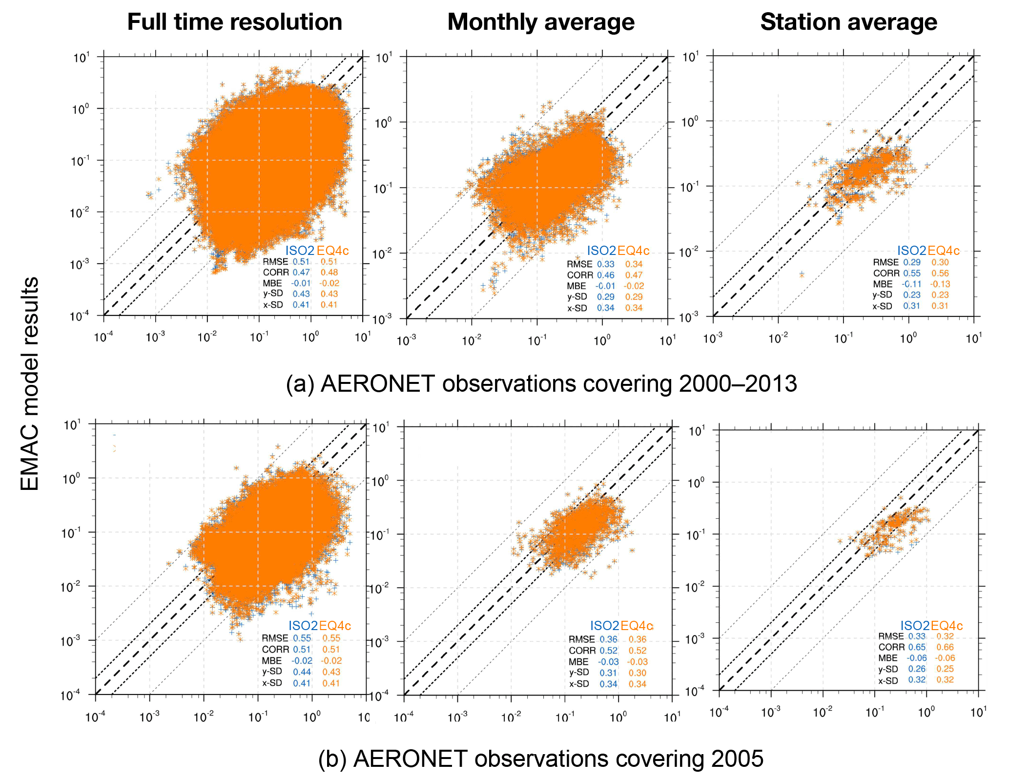
Figure 9EMAC AOD versus AERONET observations for the period 2000–2013 (a) and the year 2005 (b). Different time averages are shown for the results of ISORROPIA II (ISO2) and EQSAM4clim (EQ4c) based on 537 AERONET station locations (Fig. S1).
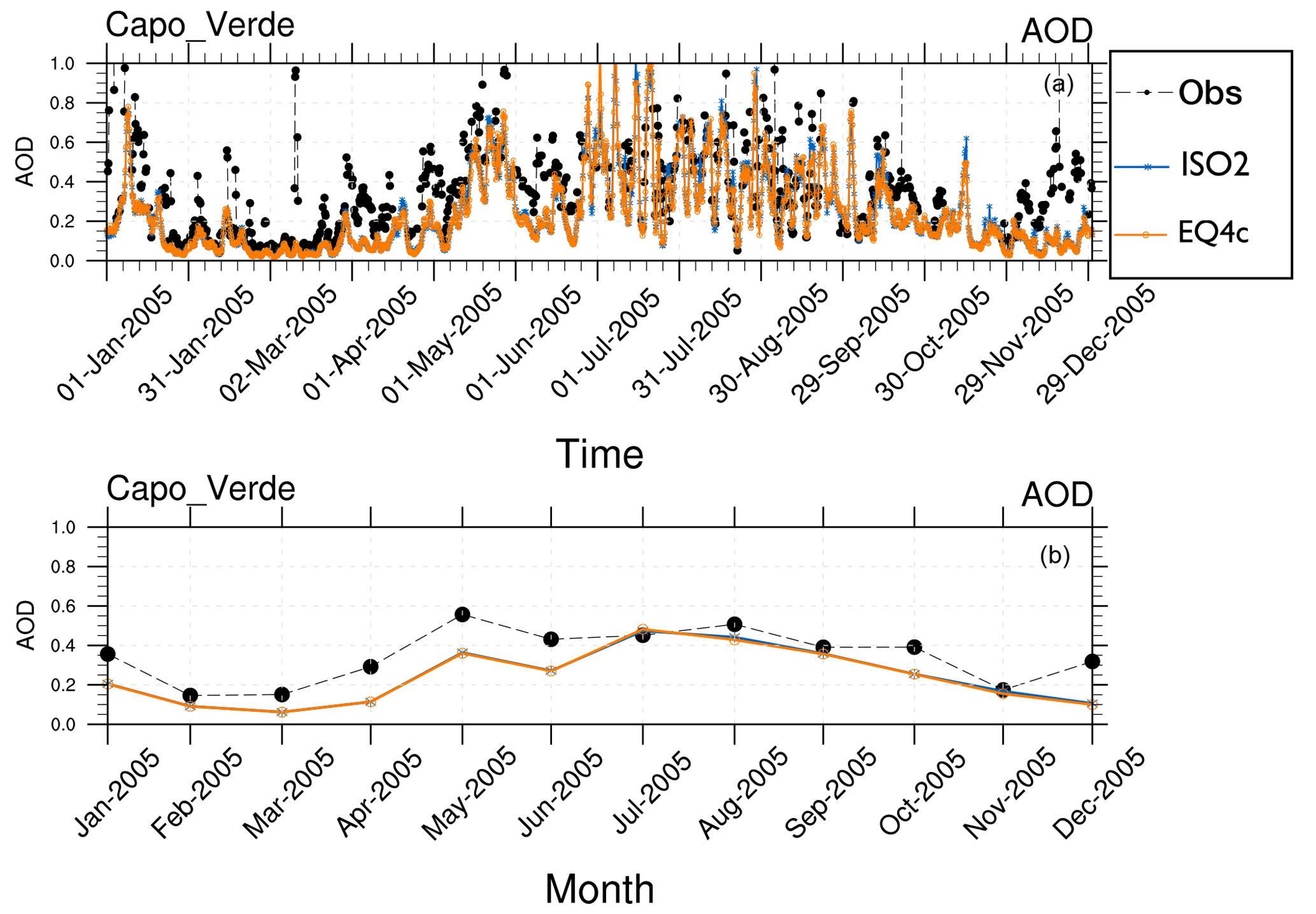
Figure 10EMAC AOD results versus AERONET observation (Obs) at Cabo Verde (year 2005) with (a) 5-hourly means and (b) monthly means for EQSAM4clim (EQ4c) and ISORROPIA II (ISO2).
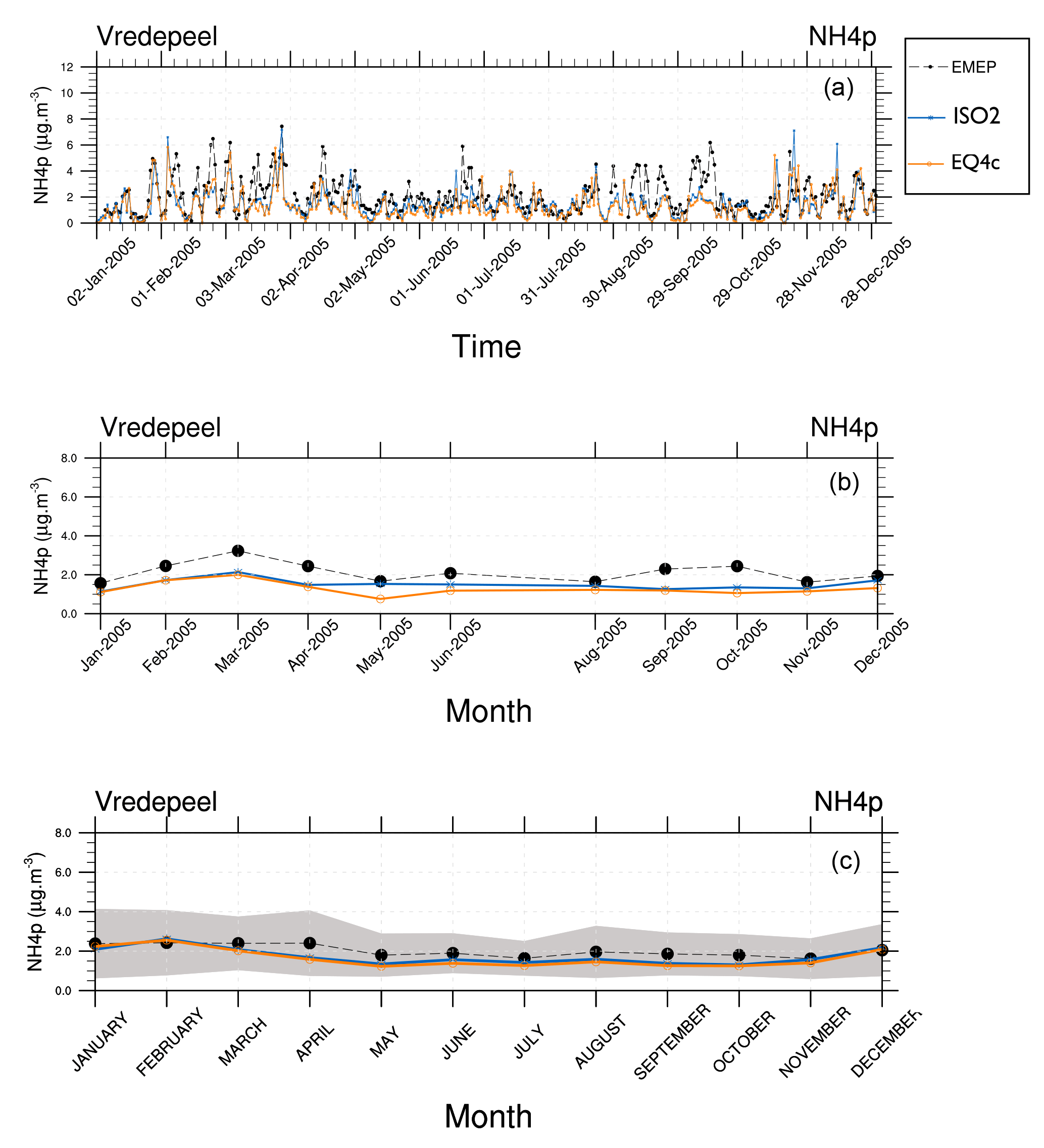
Figure 11Total (liquids and solids) particulate ammonium () at the EMEP site Vredepeel for the year 2005. Daily means (a), monthly means (b), climatological year based on the 14-year monthly mean (c). ISORROPIA II (ISO2) and EQSAM4clim (EQ4c) versus observations (EMEP).
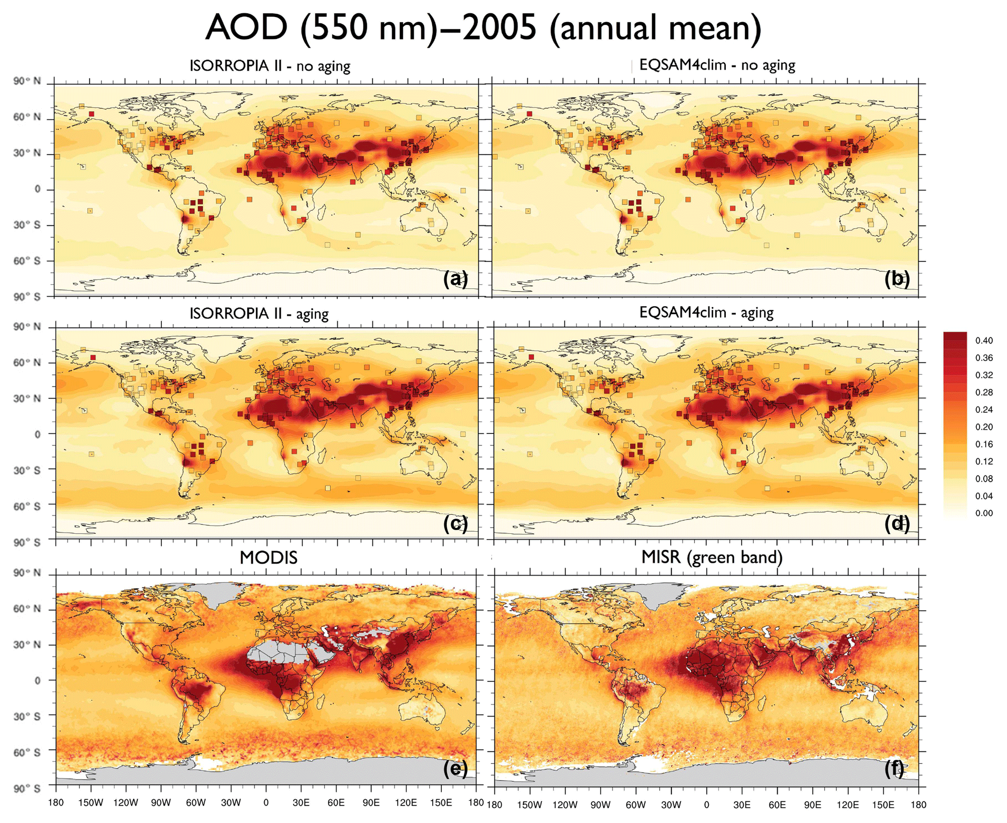
Figure 12EMAC model AOD results for the year 2005 (annual mean) based on ISORROPIA II (a, c) and EQSAM4clim (b, d). (a, b) No aging and (c, d) aging cases. AERONET ground station observations are included as squares (same color scale). (e, f) Satellite observations by MODIS (e) and MISR (f) (550 nm, annual mean 2005). MODIS monitors the ambient AOD from space and provides data over the oceans and, except deserts, also over continents (http://modis-atmos.gsfc.nasa.gov/, last access: 23 November 2018). The MISR aerosol product is available globally (products can be obtained from http://disc.sci.gsfc.nasa.gov/giovanni, last access: 23 November 2018).
To consider the hysteresis effect in a climate model, we assume for the sake of simplicity (and because of missing measurements) no single compound efflorescence thresholds. Our criteria that determine a wet case or dry case instead depend on two factors: (i) a RH threshold and (ii) the existence of aerosol water mass from the previous time step. In case aerosol water mass from the previous time step is nonzero for the given time step (and model grid box), and, if additionally the RH is above 40 % (fixed efflorescence value), we consider the upper hysteresis loop and only calculate the gas–liquid partitioning with either EQSAM4clim or ISORROPIA II. Otherwise, we account for the full gas–liquid–solid partitioning (lower hysteresis loop). The water uptake is then based on deliquescence of single or mixed solutions as described in Metzger et al. (2016a). Note that the aerosol water mass is treated prognostically in our EMAC version Sect. 2.5. That is, we assign a model tracer for water vapor and for each aerosol mode to transport the different water masses. This allows us to retrieve the required time information for a certain location on Earth, although we are only approximately able to distinguish between the upper or lower hysteresis loop. Results of our EMAC setup that include the hysteresis effect are shown in Sects. 3 and 4.
To evaluate the hygroscopic growth calculations of EQSAM4clim and ISORROPIA II and to evaluate our EMAC version, we focus on the AOD since long-term observations are available for many regions of the Earth. The AOD, or extinction coefficient, is a measure of radiation scattering and absorption at different wavelengths and sensitive to gas–liquid–solid partitioning and aerosol hygroscopic growth. We use ground station observations from the AErosol RObotic NETwork (AERONET, http://aeronet.gsfc.nasa.gov, last access: 23 November 2018). Complementarily, we use independent satellite observations from MODIS and MISR (both available from http://disc.sci.gsfc.nasa.gov/giovanni, last access: 23 November 2018). The comparison of model results against measurements includes the in situ observations of the Clean Air Status and Trends NETwork (CASTNET, http://www.epa.gov/castnet, last access: 23 November 2018). CASTNET is a national air quality monitoring network of the United States of America designed to provide data to assess trends in air quality, atmospheric deposition, and ecological effects due to changes in air pollutant emissions. For Europe, we use data of the European Monitoring and Evaluation Programme (EMEP) (http://www.emep.int/, last access: 23 November 2018). EMEP is a scientifically based and policy-driven program under the Convention on Long-range Transboundary Air Pollution (CLRTAP) for international cooperation to solve transboundary air pollution problems (Tørseth et al., 2012). Our EMAC model evaluation is based on two model resolutions, i.e., T42 and T106 (Sect. 2.1). Most of our model output is based on 5-hourly averages, such that any full hour serves as an averaging-interval center once within 5 days. An extension of our study to a more in-depth evaluation of the underlying aerosol composition and neutralization levels will be presented separately, while the sensitivity of the inorganic aerosol composition to model assumptions (e.g., ISORROPIA II vs. EQSAM4clim) is presented in the Supplement of this work (see Sect. S1.3, Figs. S6–S20).
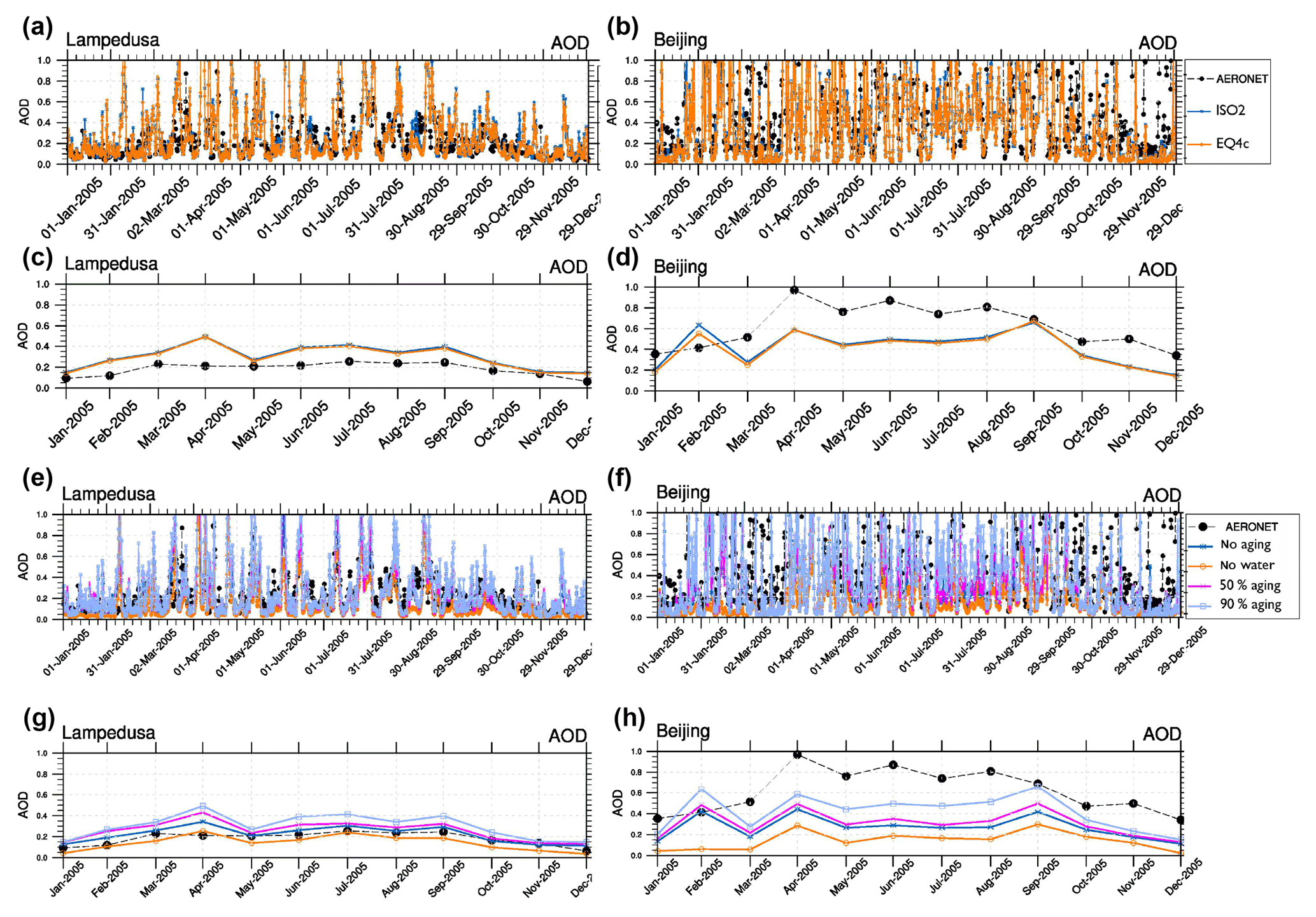
Figure 13EMAC AOD results versus AERONET observations at Lampedusa and Beijing (shown in Fig. 2) for the year 2005. The first and third rows show 5-hourly means; the second and third rows show monthly means. Panels (a) and (b) show EQSAM4clim (EQ4c) and ISORROPIA II (ISO2). Panels (g) and (h) show sensitivity of EMAC AOD to different water assumptions considering different EMAC setups: no aging (blue stars), no water without aerosol water (orange circles), 50 % aging (pink crosses), and 90 % aging (light blue squares); see Tables 4 and 2 (Sect. 4.2). The sensitivity is based on ISORROPIA II.
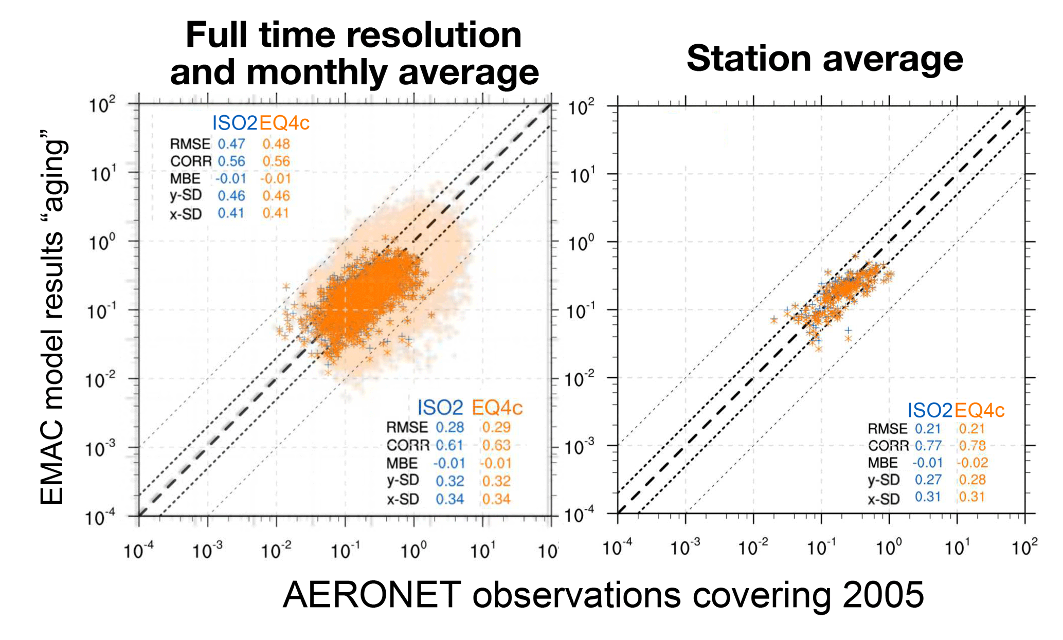
Figure 14EMAC AOD based on the aging setup versus AERONET observations for the year 2005, complementing Fig. 9. Different time averages (full time resolution in light colors with statistics in the upper left corner) are shown for the results of ISORROPIA II (ISO2) and EQSAM4clim (EQ4c) based on 537 AERONET station locations (shown in Fig. S1).
3.1 EMAC AOD versus AERONET and satellites
The EMAC hygroscopic growth calculations of EQSAM4clim and ISORROPIA II are first compared to independent AOD results of Pozzer et al. (2015) (PO2015) for the period 2000–2010. To give a compact but representative picture of our analysis, we focus on a selection of AERONET stations that represent different regions of the Earth. Figure 1 shows the selected station locations, Fig. S1 the corresponding regions. Figure 2 shows the results of the AOD comparison (from left to right, top to bottom): GSFC (North America), Sao Paulo (South America), Cape San Juan (Latin America), Cabo Verde (West Africa), Canberra (Australia), Yekaterinburg (Siberia), Forth Crete (EMME), Dakar (West Africa), Yakutsk (Siberia), Amsterdam Island (Indian Ocean), Lampedusa (North Africa), and Beijing (East Asia). Figure 3 shows the corresponding Taylor diagrams (standard deviation and correlation coefficient) of the AOD comparison of EQSAM4clim, ISORROPIA II, and PO2015. The comparison includes different observations from independent satellite instruments, i.e, MODIS, MODIS-Aqua, MODIS-Deep Blue, MISR, SeaWIFS, and ENVISAT, which are discussed in detail in our extended evaluation study. All satellite products and model results are compared against the AERONET observations for the period 2000–2010 (based on globally averaged seasonal means using a 5-hourly model output and accordingly averaged AERONET observations – details are given in Metzger et al. (2016b), which also outlines our interpolation procedure in time and space). The corresponding scatter plots are shown in Figs. S2–S4 and include the statistics root-mean-square error (RMSE), correlation coefficient (R), mean biased error (MBE), standard deviation of the model results (σm), and AERONET observations (σo). The equations are given in Appendix A: Evaluation metrics.
The comparison shows that the differences associated with the two partitioning schemes are smaller compared to the differences associated with the two different EMAC setups, i.e., our EMAC version with EQSAM4clim (orange circles) and ISORROPIA II (blue stars), and the independent PO2015 setup (pink crosses). But all AOD model results are relatively close to the AERONET observations, despite the distinct different underlying approaches to obtain the mixed-solution aerosol water uptake. The largest differences occur for regions that are dominated by mineral DU outbreaks, as indicated by the AERONET stations Cabo Verde and Dakar (Fig. 2). The reason is that PO2015 uses prescribed DU emissions, while our setup calculates the DU emission fluxes online with the EMAC meteorology (Sect. 2.4). Although the same is true for the SS emissions, differences there are much less pronounced (see, for example, Amsterdam Island). The prescribed DU emissions basically yield a mean DU concentration with a too low variability, which is reflected in a too low variability in the AOD results (see pink crosses for Dakar in Fig. 2, for example). Conversely, our EMAC version results show too low minimum values for certain periods (e.g., for 2002–2008), but the magnitude of the seasonal cycle is much closer to the AERONET observations (black circles). Conversely, the setup of PO2015 is based on the T106L31 resolution (), while our results are based on a T42L31 () setup. Although the coarser resolution somewhat affects the statistics of the analysis (see Supplement), our results are also within the range of the satellite results when compared to the AERONET observations (Fig. 3). Notably, spring and summer seasons are better resolved than the winter months for our T42L31 setup. Altogether the results indicate that we may underestimate the chemical aging of bulk particles, which is therefore scrutinized in Sect. 4.2.
3.2 EQSAM4clim versus ISORROPIA II for 2000–2013
To further evaluate EQSAM4clim and ISORROPIA II, we compare the AOD and the total particulate matter (PM) that drives the model AOD with AERONET and EMEP observations for the period for 2000–2013. Figure 4 shows that the AOD and PM time series and the climatological year (14-year average) are close to independent observations of the EMEP station Harwell and the AERONET site Chilbolton (United Kingdom, Fig. 1). The two sites lie within one model grid box and are chosen since no other site provides long-term observations of both AOD and PM. Only Cabauw in the Netherlands, which is one of the few EMEP and AERONET super-sites, provides AOD and PM observations with some reasonable overlap and supports these results as shown in Fig. 5. To complement the picture, the corresponding aerosol water (H2O), which is associated with the total model PM, is also shown yielding consistent results for EQSAM4clim and ISORROPIA II (but no observations are available).
Figure S5 (Sect. S1.2) shows the corresponding size-resolved PM, aerosol water, number concentration, and wet radius for each aerosol mode: nucleation soluble (ns), Aitken soluble (ks), accumulation soluble (as), coarse soluble (cs), Aitken insoluble (ki), accumulation insoluble (ai), and coarse insoluble (ci) for ISORROPIA II (left column) and EQSAM4clim (right column). The sum of the modes (for PM, H2O) is identical to Fig. 5 and also supports this finding. Figure 6 further shows various PM time series of EQSAM4clim and ISORROPIA II (top panels) in comparison with EMEP stations, which provide long-term PM observations, i.e., Cabo de Creus, Hyytiälä, Illmitz, and Vredepeel. The station locations are shown in Fig. 1, the corresponding climatological year below each time series (Fig. 6). Interestingly, despite the distinct different regions and climates, our EMAC model results are close to these long-term PM observations. The corresponding global aerosol PM and associated water (H2O) distributions (14-year average) are shown in Figs. 7 and 8: meridional means (left columns), zonal means (middle columns), surface distributions (right columns), ISORROPIA II (ISO2, top row), EQSAM4clim (EQ4c, middle row), and together with the differences between both simulations (EQ4c–ISO2, bottom row). Notably, our water mass results are lowest in the western desert of the US in agreement with Liao (2005) and Carlton and Turpin (2013), for example.
Importantly, both the AOD and PM model results nicely compare with various surface observations for the entire evaluation period (2000–2013). However, the global surface and vertical distributions from both EMAC simulations are also in close agreement for the aerosol PM and H2O, which supports our previous finding (Sect. 3.1) that the difference between EQSAM4clim and ISORROPIA II is negligible on climate simulation timescales. Figure 9 additionally shows scatter plots of the model AOD versus AERONET observations for the period 2000–2013 and the year 2005. For each period, three different time averages are shown, i.e., 5-hourly averages (full time resolution), monthly means, and station means based on 537 AERONET stations all over the Earth (locations are shown in Fig. S1). The statistics included in each panel summarize the results and show that both EMAC simulations are comparable in terms of statistical key metrics, i.e., RMSE, standard deviation (σ), R, and MBE (equations are given in Appendix A). Interestingly, the statistics of all time averages indicate that the results of EQSAM4clim are slightly closer to the AERONET observations compared to ISORROPIA II. Note that Fig. 14 complements Fig. 9 with the results for 2005 with our EMAC aging setup that is discussed further in Sect. 4.2.
3.3 EQSAM4clim versus ISORROPIA II for 2005
In order to scrutinize this result, we zoom into a single location and compare the EMAC AOD of EQSAM4clim and ISORROPIA II for the AERONET observations at Cabo Verde for both 5-hourly and monthly averages (Fig. 10). Cabo Verde is one of the more difficult stations because of the frequent Sahara DU outflows (Abdelkader et al., 2017). In our setup the DU outflow is associated with elevated calcium loadings, which can cause differences in the subsequent sulfate–bisulfate neutralization (Sect. 4). Despite the slight underestimation of the AOD observations by both model simulations, the results of EQSAM4clim and ISORROPIA II are very close throughout the year. Even the distinct AOD peaks in May, which can be attributed to Saharan DU outbreaks, are well resolved at the 5-hourly output frequency, although the comparison based on monthly averages seems to be less impressive. Nevertheless, the absolute comparison is overall very good for a chemistry–climate model.
To evaluate the aerosol composition that drives the hygroscopic growth, we further compare our aerosol ammonium () results against EMEP observations at the measurement site Vredepeel. is the weakest cation considered in our simulations and driven out of the aerosol phase by all nonvolatile cations because of its semi-volatility. It is one of the most difficult aerosol species to model, if the mineral cations Na+, K+, Mg2+, and Ca2+ are considered, for example, through a chemical speciation of the aerosol emission fluxes (Sect. 2.4). For cation-rich locations therefore shows the largest sensitivity in our aerosol calculations (shown by the results of Sect. S1.3, for example). Only in the case that is the only cation that neutralizes the anions , , , and Cl−, is it preferentially bound with sulfate for which the aerosol concentrations are usually in good agreement with observations. However, including mineral cations through a chemical speciation of emission fluxes complicates the modeling enormously. Despite these challenges, our comparison with observations in Fig. 11 shows that the total particulate ammonium, i.e., the sum of all liquid and solid cations, compares well for different time averages for the year 2005. Differences between EQSAM4clim and ISORROPIA II are also rather small for the daily, monthly, and even 14-year monthly mean (climatological year).
To further evaluate our EMAC results on a global scale, Fig. 12 compares the annual mean AOD of ISORROPIA II (left panels) and EQSAM4clim (right panels) against AERONET observations (included as squares) for 2005 (top and middle rows). The top row represents our no aging case and excludes chemical aging and hysteresis effects (Sect. 4.1), while the middle row represents our aging case and includes both effects (they are discussed further in Sect. 4.2). The bottom row shows independent satellite observations from MODIS and MISR. Altogether, this comparison shows that the EMAC results based on EQSAM4clim and ISORROPIA II are also very similar on a global scale and that the EMAC results labeled aging compare better with the satellite observations than the no aging results. This qualitative comparison indicates that the overall assumption on the water uptake is important. But it also shows that the differences between the two different EMAC setups (comparing upper and middle row) are larger than the differences between the two distinct different gas–aerosol partitioning schemes (comparing left and right panels).
To scrutinize the importance of the aerosol water calculations, we compare our EMAC results in a sensitivity study that excludes (Sect. 4.1) and includes (Sect. 4.2) the aerosol water and bulk water uptake (Sect. 2.5) due to the chemical aging of primary particles (Sect. 2.4).
4.1 EMAC setup – without chemical aging of bulk species
Our EMAC setup without chemical aging omits the water uptake of bulk aerosols (OC, BC, SS, DU) in contrast to the aging case (Sect. 4.2), which considers that the bulk particle hygroscopicity can change with time (Sect. 2.5). For both setups we consider the chemical speciation of the emission fluxes (Sect. 2.4) to obtain chemically specified aerosol mass fractions in terms of cations and anions. But for the no aging case, we limit the water uptake to the neutralization products (ion pairs), which are calculated with the partitioning schemes (Sect. 2.3). Our reasoning for this limited setup is that the aerosol water mass of bulk species (Sect. 2.5), as well as the hysteresis effect (Sect. 2.6), can regionally reduce potential differences of the aerosol water mass calculations if the total aerosol water mass is dominated by one of these effects. For both processes explicit RHD calculations and the associated uncertainties (Metzger et al., 2016a) are excluded. The no aging setup is therefore most sensitive to potential differences in the water uptake calculation approaches of EQSAM4clim and ISORROPIA II, though differences are rather small on a global scale as discussed in Sect. 3.3 (i.e., shown by the comparison in Fig. 12a, b).
We note that the relatively largest deviations occur in our no aging EMAC setup for stations that are subject to high DU loads, e.g., Dakar and Cabo Verde (see Supplement). But the aerosol properties that are most important for climate modeling, i.e., the total (dry) PM and the associated aerosol water mass concentrations, are mostly close to a one-by-one line for all simulations and all stations. Differences are mainly caused by differences in the bisulfate–sulfate partitioning of both schemes. In contrast to ISORROPIA II, EQSAM4clim does not treat the dissolution of weak acids (HNO3, HCl) and bases (NH3), which can cause differences in the sulfate neutralization levels and the subsequent water coating of mineral DU particles. The Kelvin effect is also not considered in ISORROPIA II in contrast to EQSAM4clim, which can have an effect on the water uptake of Aitken mode but not coarser particles. Nevertheless, overall differences are small in terms of mass concentrations as shown by the extended analysis included in the Supplement.
Note that the Supplement (Sect. S1.3) shows both time series and scatter plots for 2005 for our no aging case, which are based on all 537 AERONET stations of Fig. S1. The results include the PM (Fig. S6) and H2O (Fig. S7) concentrations [µg m−3(air)], as well as those of the lumped aerosols, i.e., sulfate (), bisulfate (), nitrate (), chloride (Cl−), ammonium (), sodium (Na+), potassium (K+), magnesium (Mg2+), and calcium (Ca2+), shown in Figs. S8–S16. The corresponding scatter plots (Figs. S17–S20) show the annual means for three soluble (key) aerosol modes of GMXe (Sect. 2.2): coarse (top row), accumulation (middle row), and Aitken (bottom row) and include the growth factor (GF; see Metzger et al., 2016a). Each panel includes the statistics RMSE, R, MBE, and standard deviation of ISORROPIA II (x-SD) and EQSAM4clim (y-SD). Table 3 complements the time series and scatter plots with some additional statistics of key EMAC tracers.
4.2 EMAC setup – with chemical aging of bulk species
The EMAC setup labeled aging extends the no aging setup (Sect. 4.1) with the water mass calculation of bulk aerosol species and the hysteresis effect (Sect. 2.6) such that the bulk particle hygroscopicity can change with time (Sect. 2.5) – note Table 4. Both can become regionally important. As noted in Sect. 3.3, our EMAC aging setup compares better with observations than the no aging case. This is especially true for regions over the open oceans, intense biomass burnings, or DU outbreaks, including the transatlantic DU transport as shown in Fig. 12. But despite the more complex chemical aging setup of bulk species, our EMAC version still somewhat underestimates the AOD observations. This finding is supported by the AERONET observations, which are included in Fig. 12 (squares with the same color scale). One reason could be that our default aging setup only considers a partial aging of 50 % of the bulk aerosol mass for the additional water uptake calculations.
To scrutinize the effect of aging level on the AOD comparison, we apply different levels of bulk aging according to Table 4. Figure 13 shows the results of four different EMAC simulations, i.e., case 1 with no aging (blue stars), case 2 with no water (orange circles), case 3 with 50 % aging (pink crosses), and case 4 with 90 % aging (light blue squares). The upper two rows compare the model results of EQSAM4clim and ISORROPIA II based on case 4 for the AERONET observations at Lampedusa and Beijing for the year 2005. The first and third rows show the 5-hourly means, while the second and fourth rows show the corresponding monthly means. The lowest two rows present the key results of our sensitivity study.
The comparison of cases 1–4 shows that aerosol water calculations are essential. Excluding aging or aerosol water at all, our EMAC simulation largely underestimates the AOD (case 1–2), while considering the bulk water uptake (aging case 3–4) improves the AOD comparison. However, the improvement strongly depends on the AERONET location and the assumed level of aging. For instance, our EMAC results based on a 90 % aging level (case 4) can overestimate the AOD observations at certain locations such as for Lampedusa, while at the same time the results compare best with other observations such as at the AERONET site of Beijing. With a decreasing level of aging, the AOD observations become more underestimated for Beijing, while they are improved for Lampedusa. This fact points to missing processes that cannot be resolved by applying constant chemical aging parameters. To improve our results further, a more comprehensive chemical aging parameterization is needed by an extension of the water uptake framework to organic compounds as considered by Metzger and Lelieveld (2007), for example. This study included the neutralization of major carboxylic acids for neutralization by the cations Na+, K+, Ca2+, and Mg2+ to form salt compounds (formates, acetates, oxalates, citrates; see their Table 1), which can contribute to the overall aerosol water mass and hence regionally improve the AOD. Yet, such extensions are beyond the scope of this work. Here, we focus on a consistent model intercomparison of EQSAM4clim and ISORROPIA II and the importance of aerosol water mass for the model evaluation in terms of AOD. Nevertheless, our EMAC results based on the higher aging level (case 4) improve the global-scale comparison of Fig. 9 (discussed in Sect. 3.2) as shown by Fig. 14. Note that the hysteresis assumption (Sect. 2.6) comes on top of both, i.e., our aging and no aging (Sect. 4.1) assumption, but is negligible in our EMAC setup compared to the aging effect, which is why we have not separated it from the sensitivity analysis. Thus, the differences in AOD between aging and no aging are basically caused by the associated water uptake of bulk compounds (SS, DU, OC, BC).
Overall, our sensitivity analysis indicates the potential limitations associated with the lack of water uptake on organic aerosol, the effects of organic aerosol on inorganic partitioning and resulting water uptake, and water uptake and resulting AOD. With Fig. 13 we show the results of different aging assumptions. Although we do not explicitly treat organic aerosols, the 50 % and 90 % aging cases also include water uptake of organic aerosols through our consideration of OC bulk mass (with the parameters given in Table 2). Clearly, only certain regions are dominated by organic aerosols and the water uptake of organic aerosols is usually much less than that of the inorganic counterparts (if normalized to the aerosol mass). Nevertheless, certain regions such as Beijing can be dominated by organic aerosols and the effect on AOD can be significant as shown by Fig. 13 – compare no water without aerosol water (orange circles), 50 % aging (pink crosses), and 90 % aging (light blue squares) for the monthly means.
4.3 Importance of aerosol water
The sensitivity of our AOD calculations with respect to the RH cutoff is analyzed next. Such a cutoff is required for all aerosol water mass calculations and applied to prevent overlap between aerosol hygroscopic growth and parameterized cloud formation. Most of our EMAC simulations use a default cutoff (maximum) RH = 95 or 98 %, while there is no minimum RH by default. In our EMAC simulations the minimum RH is determined automatically by the aerosol composition, i.e., by the single solute or mixed-solution deliquescence RH (this is detailed in Sect. 2.6 of Metzger et al., 2016a).
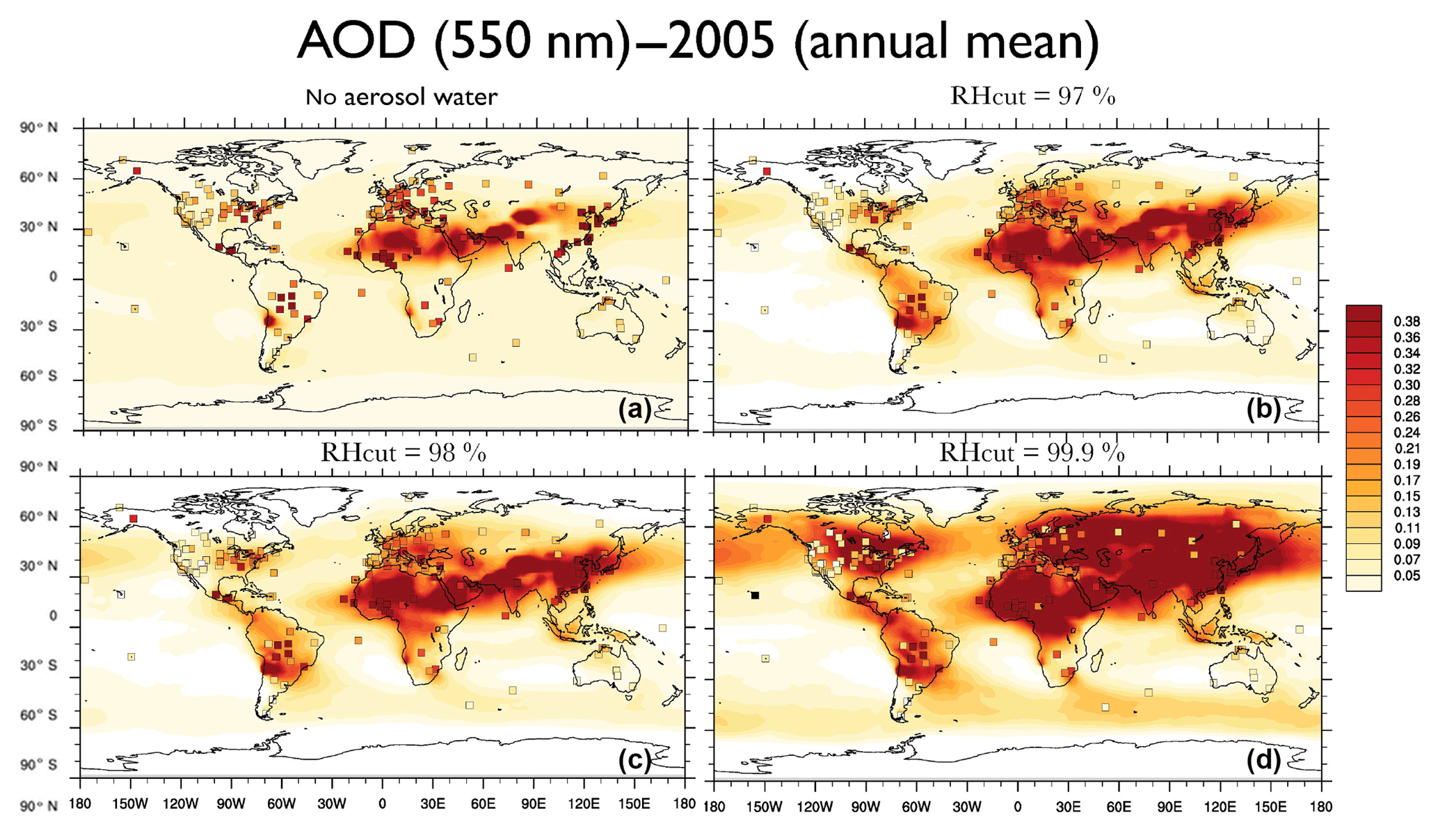
Here we consider four different RH cutoff cases for which AOD results (2005, annual mean) of four EMAC simulations are shown in Fig. 15 (from left to right, top to bottom): (a) RH = 0 [%], i.e., no aerosol water; (b) RH =97 [%]; (c) RH = 98 [%]; and (d) RH = 99.9 %. The four simulations only differ by the assumption on the aerosol water uptake limitation, i.e., the upper RH value that is used to limit the water uptake calculation for both EQSAM4clim and ISORROPIA II. While our first and last sensitivity simulations represent an extreme case (with unrealistic AOD results), the two simulations with RH = 97 and 98 % cutoffs yield similar AOD results that are relatively close to many AERONET observations (colored squares). Noticeably, the AOD values significantly increase for the high RH = 99.9 % case. Of course, any RH cutoff is arbitrary if the aerosol water mass is not consistently linked with cloud formation. To avoid an inconsistent aerosol–cloud–radiation coupling, Metzger and Lelieveld (2007) proposed a mass conservative coupling to limit the aerosol water mass by an approach that needs to be further scrutinized too (presented elsewhere).
The importance of aerosol water for AOD calculations has been scrutinized by a long-term evaluation of EQSAM4clim and ISORROPIA II on climate timescales using our EMAC model version as applied in Abdelkader et al. (2015), Metzger et al. (2016a, b), and Abdelkader et al. (2017). Generally, the results of both gas–liquid–solid partitioning schemes are in good agreement despite differences in the bisulfate partitioning and mixed-solution deliquescence humidity range, for which the results of thermodynamic schemes are typically associated with deviations (Metzger et al., 2016a). However, these discrepancies are negligible for climate simulations, as the total aerosol water mass and AOD do not significantly differ. Furthermore, in addition to the relative importance of (a) the general model setup (EQSAM4clim or ISORROPIA II), (b) number and types of compounds considered for the aerosol water calculations (e.g., mineral cations), (c) water uptake by bulk species and chemical aging, and (d) hysteresis effect (efflorescence versus deliquescence), it appeared that (e) the aerosol water uptake limitations of both partitioning schemes are most determinant for AOD calculations. Overall, the comparison of our EMAC results with remote-sensing AOD observations reveals the importance of the aerosol water calculations for climate applications.
EQSAM4clim is freely available for research and noncommercial applications. For commercial applications special licensing applies. For both cases, please contact the author (swen.metzger@researchconcepts.io). The Modular Earth Submodel System (MESSy) is continuously further developed and applied by a consortium of institutions. The usage of MESSy and access to the source code is licensed to all affiliates of institutions that are members of the MESSy Consortium. Institutions can become members of the MESSy consortium by signing the MESSy Memorandum of Understanding, see the MESSy website (https://www.messy-interface.org, last access: 23-11-2018).
Root-mean-square error
Standard deviation
Correlation coefficient
Mean biased error (MBE)
Index m refers to the model (EQSAM4clim or ISORROPIA II) and o to observations (or ISORROPIA II in the case of a model–model comparison).
Computational efficiency is a key constraint on our model development. To scrutinize the model performance, we compare both gas–aerosol partitioning schemes (EQSAM4clim and ISORROPIA II) using the simulation period of 2005. Table 5 presents the computational burden (CPU times) for different EMAC simulations (T42L31). Experiments A, B, C, and D correspond to a no aging EMAC setup (results of Exp. A and B are shown in Sect. S1.3). The four simulations only differ by the constraint on the gas–aerosol partitioning scheme; i.e., Exp. A represents ISORROPIA II, Exp. B and C represent two simulations of EQSAM4clim (identical setup, just quantifying numerical noise of the computing architecture), while for Exp. D the call to the gas–liquid–solid partitioning scheme has been commented out, while all other GMXe processes remained unchanged (Sect. 2.2). Exp. D therefore represents the minimum of CPU time that is required for our GMXe aerosol setup on the Cy-Tera supercomputer (http://web.cytera.cyi.ac.cy, last access: 23 November 2018). Two additional experiments, labeled Exp. A0 and Exp. B0, represent sensitivity simulations of ISORROPIA II and EQSAM4clim, respectively. Both only omit anthropogenic emissions in our EMAC setup, while all other EMAC processes remained the same as for Exp. A and B.
Table 5 reveals the real CPU utilization. The comparison of the numbers shows (i) a dependency of both partitioning schemes on the aerosol setup and composition (Exp. A versus A0 and Exp. B versus B0), (ii) that the dependency of the additional computational costs for EQSAM4clim in addition to GMXe is small (Exp. B and C versus Exp. D and B0 versus D), while (iii) this is not so much the case for ISORROPIA II (Exp. A versus D and A0 versus D). Given the uncertainty in these numbers due to the different system loads (indicated by Exp. B versus C), the additional computational cost of EQSAM4clim is clearly negligible for climate applications on architecture such as of the Cy-Tera cluster (Intel Westmere X5650 processors, two hexa-core sockets per node). But the differences depend on the system and its usage and are generally smaller on pure scalar architectures. On typical vector machines, however, these differences can significantly increase since the optimization of a short code can be much more effective. For instance, for the previous supercomputer system at the German Climate Research Center (DKRZ, https://www.dkrz.de, last access: 23 November 2018), the gain in CPU time has been about an order of magnitude. The fraction of the total EMAC CPU burden for a 2-month simulation was about 20 % for ISORROPIA II, while EQSAM4clim contributed less than 2 % (both on 128 CPUs@“Blizzard”, i.e., IBM Power6 and measured with Scalasca, http://www.scalasca.org/, last access: 23 November 2018).
EQSAM4clim has the advantage of being a short Fortran 90 code with approximately 850 lines, including comments (or about eight pages; see Appendix of Metzger et al., 2016a). For comparison, ISORROPIA II roughly counts 36 300 lines (or approx. 360 pages). This is about one-third of the entire source code of the EMAC underlying climate code (ECHAM5.3.02), which has about 119 900 lines of Fortran 90 code (also including comments). It should be emphasized that ISORROPIA II was developed for air quality rather than climate modeling, and we offer EQSAM4clim as an alternative for computationally demanding climate simulations.
| List of names and abbreviations | |
|---|---|
| Abbreviation | Name |
| AERONET | AErosol RObotic NETwork (http://aeronet.gsfc.nasa.gov, last access: 23 November 2018) |
| AOD | Aerosol optical depth (https://earthobservatory.nasa.gov/global-maps, last access: 23 November 2018) |
| CPU | Computational performance unit (https://en.wikipedia.org/wiki/Central_processing_unit, last access: 23 November 2018) |
| Cy-Tera | The Cyprus Institute high-performance computing system (http://web.cytera.cyi.ac.cy/, last access: 23 November 2018) |
| DKRZ | The German Climate Computing Center high-performance computing system (https://www.dkrz.de, last access: 23 November 2018) |
| EMAC | ECHAM5/MESSy Atmospheric Chemistry-climate model (Joeckel et al., 2005, 2006a, b, 2008, 2010, 2016) |
| EQSAM4clim | Equilibrium Simplified Aerosol Model (Version 4) for Climate Simulations (Metzger et al., 2016a, b) |
| GMXe | Aerosol microphysics model, Global Modal-aerosol eXtension (Pringle et al., 2010a, b) |
| ISORROPIA II | Equilibrium Aerosol Model (Fountoukis and Nenes, 2007; Nenes et al., 1998) |
| MODIS | Satellite observations (http://modis-atmos.gsfc.nasa.gov/, last access: 23 November 2018) |
| MISR | Global satellite data (https://giovanni.gsfc.nasa.gov/giovanni/, last access: 23 November 2018) |
| Scalasca | Performance measuring software tool (http://www.scalasca.org/, https://bit.ly/2GF5IoB, last access: 23 November 2018) |
The supplement related to this article is available online at: https://doi.org/10.5194/acp-18-16747-2018-supplement.
SM wrote the paper and performed the simulations, with support of MA, BS and KK. Particularly, MA contributed with data analysis and plotting, BS with EMAC support and KK with dust emission updates.
The authors declare that they have no conflict of interest.
This article is part of the special issue “The Modular Earth Submodel System (MESSy) (ACP/GMD inter-journal SI)”. It is not associated with a conference.
This work was supported by the European Research Council under the European
Union's Seventh Framework Programme (FP7/2007-2013)–ERC grant agreement no.
226144 through the C8 Project, and by the Energy oriented Centre of
Excellence (EoCoE), grant agreement number 676629, funded within the
Horizon 2020 framework of the European Union. EMAC simulations have been
carried out on the supercomputer of the German Climate Research Center and on
the Cy-Tera cluster, operated by the Cyprus Institute (CyI) and co-funded by
the European Regional Development Fund and the Republic of Cyprus through the
Research Promotion Foundation (Project Cy-Tera NEA-YΠOΔOMH/ΣTPATH/0308/31). Model emissions were kindly provided by the
anthropogenic emission inventory EDGAR Climate Change and Impact Research
(CIRCE) through the EU FP6 project no. 036961. We thank the measurement and
model development teams for providing the observations, numerical models, and
many useful codes that have been used in this study.
The article processing charges for this open-access
publication were covered by the Max Planck Society.
Edited by: Rolf Müller
Reviewed by: two anonymous referees
Abdelkader, M., Metzger, S., Mamouri, R. E., Astitha, M., Barrie, L., Levin, Z., and Lelieveld, J.: Dust-air pollution dynamics over the eastern Mediterranean, Atmos. Chem. Phys., 15, 9173–9189, https://doi.org/10.5194/acp-15-9173-2015, 2015. a, b, c, d, e, f, g
Abdelkader, M., Metzger, S., Steil, B., Klingmueller, K., Tost, H., Pozzer, A., Stenchikov, G., Barrie, L., and Lelieveld, J.: Sensitivity of transatlantic dust transport to chemical aging and related atmospheric processes, Atmos. Chem. Phys., 17, 3799–3821, https://doi.org/10.5194/acp-17-3799-2017, 2017. a, b, c, d, e, f, g
Ackermann, I. J., Hass, H., Memmesheimer, M., Ebel, A., Binkowski, F. S., and Shankar, U.: Modal aerosol dynamics model for Europe, Atmos. Environ., 32, 2981–2999, https://doi.org/10.1016/S1352-2310(98)00006-5, 1998. a
Ahmadov, R. and Kazil, J.: Aerosol modeling with WRF-Chem, Tutorial WRF-Chem Tutorial, CU CIRES and NOAA Earth System Research Laboratory, https://ruc.noaa.gov/wrf/wrf-chem/wrf_tutorial_2018/Aerosols.pdf, last access: 23 November 2018. a
Astitha, M., Lelieveld, J., Abdel Kader, M., Pozzer, A., and de Meij, A.: Parameterization of dust emissions in the global atmospheric chemistry-climate model EMAC: impact of nudging and soil properties, Atmos. Chem. Phys., 12, 11057–11083, https://doi.org/10.5194/acp-12-11057-2012, 2012. a, b
Bauer, S. E., Koch, D., Unger, N., Metzger, S. M., Shindell, D. T., and Streets, D. G.: Nitrate aerosols today and in 2030: a global simulation including aerosols and tropospheric ozone, Atmos. Chem. Phys., 7, 5043–5059, https://doi.org/10.5194/acp-7-5043-2007, 2007a. a, b
Bauer, S. E., Mishchenko, M. I., Lacis, A. A., Zhang, S., Perlwitz, J., and Metzger, S. M.: Do sulfate and nitrate coatings on mineral dust have important effects on radiative properties and climate modeling?, J. Geophys. Res., 112, 1–9, https://doi.org/10.1029/2005JD006977, 2007b. a, b
Bessagnet, B., Hodzic, A., Vautard, R., Beekmann, M., Cheinet, S., Honoré, C., Liousse, C., and Rouil, L.: Aerosol modeling with CHIMERE – preliminary evaluation at the continental scale, Atmos. Environ., 38, 2803–2817, https://doi.org/10.1016/j.atmosenv.2004.02.034, 2004. a
Bian, H., Chin, M., Hauglustaine, D. A., Schulz, M., Myhre, G., Bauer, S. E., Lund, M. T., Karydis, V. A., Kucsera, T. L., Pan, X., Pozzer, A., Skeie, R. B., Steenrod, S. D., Sudo, K., Tsigaridis, K., Tsimpidi, A. P., and Tsyro, S. G.: Investigation of global particulate nitrate from the AeroCom phase III experiment, Atmos. Chem. Phys., 17, 12911–12940, https://doi.org/10.5194/acp-17-12911-2017, 2017. a, b
Binkowski, F. S. and Shankar, U.: The Regional Particulate Matter Model: 1. Model description and preliminary results, J. Geophys. Res., 100, 26191, https://doi.org/10.1029/95JD02093, 1995. a
Bruehl, C., Lelieveld, J., Crutzen, P. J., and Tost, H.: The role of carbonyl sulphide as a source of stratospheric sulphate aerosol and its impact on climate, Atmos. Chem. Phys., 12, 1239–1253, https://doi.org/10.5194/acp-12-1239-2012, 2012. a
Carlton, A. G. and Turpin, B. J.: Particle partitioning potential of organic compounds is highest in the Eastern US and driven by anthropogenic water, Atmos. Chem. Phys., 13, 10203–10214, https://doi.org/10.5194/acp-13-10203-2013, 2013. a
Darmenov, A., da Silva, A., Colarco, P., Gelaro, R., Todling, R., Bian, H., Longo, K., Castellanos, P., Nielsen, E., Buchard-Marchant, V., Randles, C., and Keller, C.: NASA Update GEOS-5 Model and Data Assimilation System: Aerosols and Clouds prsented at the International Cooperative for Aerosol Prediction (ICAP/AEROCAST) “Lidar Data and its use in Model Verification and Data Assimilation”, July 12-14, 2016, College Park, MD, USA, http://icap.atmos.und.edu/ICAP8/Day1/Darmenov_TuesdayPM.pdf, 2016. a
de Meij, A., Krol, M., Dentener, F., Vignati, E., Cuvelier, C., and Thunis, P.: The sensitivity of aerosol in Europe to two different emission inventories and temporal distribution of emissions, Atmos. Chem. Phys., 6, 4287–4309, https://doi.org/10.5194/acp-6-4287-2006, 2006. a
de Meij, A., Pozzer, A., Pringle, K., Tost, H., and Lelieveld, J.: EMAC model evaluation and analysis of atmospheric aerosol properties and distribution with a focus on the Mediterranean region, Atmos. Res., 114/115, 38–69, https://doi.org/10.1016/j.atmosres.2012.05.014, 2012. a
de Meij, A.: Uncertainties in modelling the spatial and temporal variations in aerosol concentrations, PhD Thesis, Technische Universiteit Eindhoven, 1–216 , https://doi.org/10.6100/IR642890, 2009. a
Dentener, F., Williams, J., and Metzger, S.: Aqueous Phase Reaction of HNO4: The Impact on Tropospheric Chemistry, J. Atmos. Chem., 41, 109–134, https://doi.org/10.1023/A:1014233910126, 2002. a, b
Doering, U. M., Monni, S., Pagliari, V., Orlandini, L., van Aardenne, J., and SanMartin, F.: CIRCE report D8.1.1: Emission inventory for the past period 1990–2005 on 0.1 × 0.1 grid, Tech. rep., Project FP6: 6.3 No. 036961, Joint Research Centre (JRC),http://edgar.jrc.ec.europa.eu/overview.php?v=432_GHG&SECURE=123 (last access: 23 November 2018), 2009a. a
Doering, U. M., van Aardenne, J., Monni, S., Pagliari, V., Orlandini, L., and SanMartin, F.: CIRCE report D8.1.2 – Evaluation emission database 1990–2005, Tech. rep., Project FP6: 6.3 No. 036961, Joint Research Centre (JRC),http://edgar.jrc.ec.europa.eu/overview.php?v=432_GHG&SECURE=123 (last access: 23 November 2018), 2009b. a
Doering, U. M., van Aardenne, J., Monni, S., Pagliari, V., Orlandini, L., and SanMartin, F.: CIRCE report D8.1.3 – Update of grid- ded emission inventories, addition of period 1990–1999 to 2000–2005 dataset, Tech. rep., Project FP6: 6.3 No. 036961, Joint Research Centre (JRC), http://edgar.jrc.ec.europa.eu/overview.php?v=432_GHG&SECURE=123 (last access: 23 November 2018), 2009c. a
Environ, R.: User's guide comprehensive air quality model with extensions version 6.40, Tech. rep., Ramboll, 773 San Marin Dr., Suite 2115, Novato, CA 94945, USA, 773 San Marin Drive, Suite 2115 Novato, California, 94998, https://www.ramboll.com, http://www.camx.com, 2016. a
Fountoukis, C. and Nenes, A.: ISORROPIA II: a computationally efficient thermodynamic equilibrium model for aerosols, Atmos. Chem. Phys., 7, 4639–4659, https://doi.org/10.5194/acp-7-4639-2007, 2007. a, b, c, d
Ganzeveld, L. N., van Aardenne, J. A., Butler, T. M., Lawrence, M. G., Metzger, S. M., Stier, P., Zimmermann, P., and Lelieveld, J.: Technical Note: Anthropogenic and natural offline emissions and the online EMissions and dry DEPosition submodel EMDEP of the Modular Earth Submodel system (MESSy), Atmos. Chem. Phys. Discuss., 6, 5457–5483, https://doi.org/10.5194/acpd-6-5457-2006, 2006. a
Intergovernmental Panel on Climate Change: Climate Change 2013 – The Physical Science Basis: Working Group I Contribution to the Fifth Assessment Report of the Intergovernmental Panel on Climate Change, Cambridge University Press, Cambridge, https://doi.org/10.1017/CBO9781107415324, 2014. a
Jeuken, A. B. M., Siegmund, P. C., Heijboer, L. C., Feichter, J., and Bengtsson, L.: On the potential of assimilating meteorological analyses in a global climate model for the purpose of model validation, J. Geophys. Res.-Atmos., 101, 16939–16950, https://doi.org/10.1029/96JD01218, 1996. a
Joeckel, P., Sander, R., Kerkweg, A., Tost, H., and Lelieveld, J.: Technical Note: The Modular Earth Submodel System (MESSy) – a new approach towards Earth System Modeling, Atmos. Chem. Phys., 5, 433–444, https://doi.org/10.5194/acp-5-433-2005, 2005. a, b
Joeckel, P., Tost, H., Pozzer, A., Bruehl, C., Buchholz, J., Ganzeveld, L., Hoor, P., Kerkweg, A., Lawrence, M., Sander, R., Steil, B., Stiller, G., Tanarhte, M., Taraborrelli, D., van Aardenne, J., and Lelieveld, J.: The atmospheric chemistry general circulation model ECHAM5/MESSy1: consistent simulation of ozone from the surface to the mesosphere, Atmos. Chem. Phys., 6, 5067–5104, https://doi.org/10.5194/acp-6-5067-2006, 2006a. a, b, c, d
Joeckel, P., Tost, H., Pozzer, A., Bruehl, C., Buchholz, J., Ganzeveld, L., Hoor, P., Kerkweg, A., Lawrence, M. G., Metzger, S., Sander, R., Steil, B., Stiller, G., Tanarhte, M., Taraborrelli, D., van Aardenne, J., and Lelieveld, J.: Evaluation of the atmospheric chemistry general circulation model ECHAM5/MESSy1, http://adsabs.harvard.edu/abs/2006AGUFM.A51B0073J (last access: 23 November 2018), 2006AGUFM.A51B0073J, Provided by the SAO/NASA Astrophysics Data System, 2006b. a, b
Joeckel, P., Kerkweg, A., Buchholz-Dietsch, J., Tost, H., Sander, R., and Pozzer, A.: Technical Note: Coupling of chemical processes with the Modular Earth Submodel System (MESSy) submodel TRACER, Atmos. Chem. Phys., 8, 1677–1687, https://doi.org/10.5194/acp-8-1677-2008, 2008. a, b
Joeckel, P., Kerkweg, A., Pozzer, A., Sander, R., Tost, H., Riede, H., Baumgaertner, A., Gromov, S., and Kern, B.: Development cycle 2 of the Modular Earth Submodel System (MESSy2), Geosci. Model Dev., 3, 717–752, https://doi.org/10.5194/gmd-3-717-2010, 2010. a, b, c
Joeckel, P., Tost, H., Pozzer, A., Kunze, M., Kirner, O., Brenninkmeijer, C. A. M., Brinkop, S., Cai, D. S., Dyroff, C., Eckstein, J., Frank, F., Garny, H., Gottschaldt, K.-D., Graf, P., Grewe, V., Kerkweg, A., Kern, B., Matthes, S., Mertens, M., Meul, S., Neumaier, M., Nuetzel, M., Oberländer-Hayn, S., Ruhnke, R., Runde, T., Sander, R., Scharffe, D., and Zahn, A.: Earth System Chemistry integrated Modelling (ESCiMo) with the Modular Earth Submodel System (MESSy) version 2.51, Geosci. Model Dev., 9, 1153–1200, https://doi.org/10.5194/gmd-9-1153-2016, 2016. a, b
Kaiser, J. C., Hendricks, J., Righi, M., Riemer, N., Zaveri, R. A., Metzger, S., and Aquila, V.: The MESSy aerosol submodel MADE3 (v2.0b): description and a box model test, Geosci. Model Dev., 7, 1137–1157, https://doi.org/10.5194/gmd-7-1137-2014, 2014. a
Karydis, V. A., Tsimpidi, A. P., Pozzer, A., Astitha, M., and Lelieveld, J.: Effects of mineral dust on global atmospheric nitrate concentrations, Atmos. Chem. Phys., 16, 1491–1509, https://doi.org/10.5194/acp-16-1491-2016, 2016. a
Kerkweg, A., Buchholz, J., Ganzeveld, L., Pozzer, A., Tost, H., and Joeckel, P.: Technical Note: An implementation of the dry removal processes DRY DEPosition and SEDImentation in the Modular Earth Submodel System (MESSy), Atmos. Chem. Phys., 6, 4617–4632, https://doi.org/10.5194/acp-6-4617-2006, 2006a. a
Kerkweg, A., Sander, R., Tost, H., and Joeckel, P.: Technical note: Implementation of prescribed (OFFLEM), calculated (ONLEM), and pseudo-emissions (TNUDGE) of chemical species in the Modular Earth Submodel System (MESSy), Atmos. Chem. Phys., 6, 3603–3609, https://doi.org/10.5194/acp-6-3603-2006, 2006b. a
Klingmueller, K., Steil, B., Bruehl, C., Tost, H., and Lelieveld, J.: Sensitivity of aerosol radiative effects to different mixing assumptions in the AEROPT 1.0 submodel of the EMAC atmospheric-chemistry-climate model, Geosci. Model Dev., 7, 2503–2516, https://doi.org/10.5194/gmd-7-2503-2014, 2014. a
Klingmueller, K., Pozzer, A., Metzger, S., Stenchikov, G. L., and Lelieveld, J.: Aerosol optical depth trend over the Middle East, Atmos. Chem. Phys., 16, 5063–5073, https://doi.org/10.5194/acp-16-5063-2016, 2016. a
Klingmueller, K., Metzger, S., Abdelkader, M., Karydis, V. A., Stenchikov, G. L., Pozzer, A., and Lelieveld, J.: Revised mineral dust emissions in the atmospheric chemistry-climate model EMAC (MESSy 2.52 DU_Astitha1 KKDU2017 patch), Geosci. Model Dev., 11, 989–1008, https://doi.org/10.5194/gmd-11-989-2018, 2018. a
Koo, B., Wilson, G. M., Morris, R. E., Dunker, A. M., and Yarwood, G.: Comparison of Source Apportionment and Sensitivity Analysis in a Particulate Matter Air Quality Model, Environ. Sci. Technol., 43, 6669–6675, https://doi.org/10.1021/es9008129, 2009. a
Koo, B., Metzger, S., Emery, C., Wilson, G., and Yarwood, G.: Comparing the ISORROPIA and EQSAM Aerosol Thermodynamic Options in CAMx – ITM 2018 – 36th international technical meeting on air pollution modelling and its application, 14–18 May 2018, the Lord Elgin Hotel, Ottawa, Canada, (in conjunction with the annual WMO-Gurme Meeting), https://itm2018.vito.be, [1] Ramboll, 773 San Marin Dr., Suite 2115, Novato, CA 94945, USA, [2] ResearchConcepts io GmbH, Freiburg im Breisgau, Germany, 2018. a
Lac, C., Chaboureau, J.-P., Masson, V., Pinty, J.-P., Tulet, P., Escobar, J., Leriche, M., Barthe, C., Aouizerats, B., Augros, C., Aumond, P., Auguste, F., Bechtold, P., Berthet, S., Bieilli, S., Bosseur, F., Caumont, O., Cohard, J.-M., Colin, J., Couvreux, F., Cuxart, J., Delautier, G., Dauhut, T., Ducrocq, V., Filippi, J.-B., Gazen, D., Geoffroy, O., Gheusi, F., Honnert, R., Lafore, J.-P., Lebeaupin Brossier, C., Libois, Q., Lunet, T., Mari, C., Maric, T., Mascart, P., Mogé, M., Molinié, G., Nuissier, O., Pantillon, F., Peyrillé, P., Pergaud, J., Perraud, E., Pianezze, J., Redelsperger, J.-L., Ricard, D., Richard, E., Riette, S., Rodier, Q., Schoetter, R., Seyfried, L., Stein, J., Suhre, K., Taufour, M., Taufour, M., Thouron, O., Turner, S., Verrelle, A., Vié, B., Visentin, F., Vionnet, V., and Wautelet, P.: Overview of the Meso-NH model version 5.4 and its applications, Geosci. Model Dev. Discussions, pp. 1–66, https://doi.org/10.5194/gmd-2017-297, 2018. a
Lauer, A., Hendricks, J., Ackermann, I., Schell, B., Hass, H., and Metzger, S.: Simulating aerosol microphysics with the ECHAM/MADE GCM – Part I: Model description and comparison with observations, Atmos. Chem. Phys., 5, 3251–3276, https://doi.org/10.5194/acp-5-3251-2005, 2005. a, b
Lauer, A., Eyring, V., Hendricks, J., Joeckel, P., and Lohmann, U.: Global model simulations of the impact of ocean-going ships on aerosols, clouds, and the radiation budget, Atmos. Chem. Phys., 7, 5061–5079, https://doi.org/10.5194/acp-7-5061-2007, 2007. a
Lelieveld, J., Bruehl, C., Joeckel, P., Steil, B., Crutzen, P. J., Fischer, H., Giorgetta, M. A., Hoor, P., Lawrence, M. G., Sausen, R., and Tost, H.: Stratospheric dryness: model simulations and satellite observations, Atmos. Chem. Phys., 7, 1313–1332, https://doi.org/10.5194/acp-7-1313-2007, 2007. a
Liao, H.: Global impacts of gas-phase chemistry-aerosol interactions on direct radiative forcing by anthropogenic aerosols and ozone, J. Geophys. Res., 110, 1–22, https://doi.org/10.1029/2005JD005907, 2005. a
Luo, C., Zender, C. S., Bian, H., and Metzger, S.: Role of ammonia chemistry and coarse mode aerosols in global climatological inorganic aerosol distributions, Atmos. Environ., 41, 2510–2533, https://doi.org/10.1016/j.atmosenv.2006.11.030, 2007. a
Manders, A., Ulft, B. v., Meijgaard, E. v., and Schaap, M.: Coupling of the air quality model LOTOS-EUROS to the climate model RACMO, in: Coupling of the air quality model LOTOS-EUROS to the climate model RACMO, Knowledge for Climate Programme Office, Utrecht, http://edepot.wur.nl/328070, oCLC: 911880649, 2011. a
Metzger, S. and Lelieveld, J.: Reformulating atmospheric aerosol thermodynamics and hygroscopic growth into fog, haze and clouds, Atmos. Chem. Phys., 7, 3163–3193, https://doi.org/10.5194/acp-7-3163-2007, 2007. a, b, c, d, e, f, g, h
Metzger, S., Dentener, F., Pandis, S., and Lelieveld, J.: Gas/aerosol partitioning: 1. A computationally efficient model, J. Geophys. Res., 107, 1–24, https://doi.org/10.1029/2001JD001102, 2002a. a, b, c, d, e
Metzger, S., Dentener, F., Krol, M., Jeuken, A., and Lelieveld, J.: Gas/aerosol partitioning: 2. Global modeling results, J. Geophys. Res., 107, 1–23, https://doi.org/10.1029/2001JD001103, 2002b. a, b, c
Metzger, S., Mihalopoulos, N., and Lelieveld, J.: Importance of mineral cations and organics in gas-aerosol partitioning of reactive nitrogen compounds: case study based on MINOS results, Atmos. Chem. Phys., 6, 2549–2567, https://doi.org/10.5194/acp-6-2549-2006, 2006. a, b, c, d
Metzger, S., Steil, B., Xu, L., Penner, J. E., and Lelieveld, J.: New representation of water activity based on a single solute specific constant to parameterize the hygroscopic growth of aerosols in atmospheric models, Atmos. Chem. Phys., 12, 5429–5446, https://doi.org/10.5194/acp-12-5429-2012, 2012. a, b, c, d, e, f, g
Metzger, S., Steil, B., Abdelkader, M., Klingmueller, K., Xu, L., Penner, J. E., Fountoukis, C., Nenes, A., and Lelieveld, J.: Aerosol water parameterisation: a single parameter framework, Atmos. Chem. Phys., 16, 7213–7237, https://doi.org/10.5194/acp-16-7213-2016, 2016a. a, b, c, d, e, f, g, h, i, j, k, l, m, n, o, p, q, r, s, t, u, v, w, x, y, z
Metzger, S., Abdelkader, M., Klingmueller, K., Steil, B., and Lelieveld, J.: Comparison of Metop PMAp Version 2 AOD Products using Model Data, Final Report EUMETSAT ITT 15/210839, EUMETSAT, Max Planck Institute for Chemistry, Department of Atmospheric Chemistry, http://bit.ly/2Epxf9b (last access: 23 November 2018), 2016b. a, b, c, d, e, f, g
Monahan, E. C., Spiel, D. E., and Davidson, K. L.: A Model of Marine Aerosol Generation Via Whitecaps and Wave Disruption, in: Oceanic Whitecaps, edited by: Monahan, E. C. and Niocaill, G. M., Springer Netherlands, Dordrecht,vol. 2, 167–174, https://doi.org/10.1007/978-94-009-4668-2_16, 1986. a
Myhre, G., Grini, A., and Metzger, S.: Modelling of nitrate and ammonium-containing aerosols in presence of sea salt, Atmos. Chem. Phys., 6, 4809–4821, https://doi.org/10.5194/acp-6-4809-2006, 2006. a
Nenes, A., Pandis, S. N., and Pilinis, C.: ISORROPIA: A New Thermodynamic Equilibrium Model for Multiphase Multicomponent Inorganic Aerosols, Aquat. Geochem., 4, 123–152, 1998. a, b, c
Nguyen, T. K. V., Ghate, V. P., and Carlton, A. G.: Reconciling satellite aerosol optical thickness and surface fine particle mass through aerosol liquid water: ALW AND AOT, Geophys. Res. Lett., 43, 11903–11912, https://doi.org/10.1002/2016GL070994, 2016. a
Pozzer, A., Joeckel, P., Sander, R., Williams, J., Ganzeveld, L., and Lelieveld, J.: Technical Note: The MESSy-submodel AIRSEA calculating the air-sea exchange of chemical species, Atmos. Chem. Phys., 6, 5435–5444, https://doi.org/10.5194/acp-6-5435-2006, 2006. a
Pozzer, A., de Meij, A., Pringle, K. J., Tost, H., Doering, U. M., van Aardenne, J., and Lelieveld, J.: Distributions and regional budgets of aerosols and their precursors simulated with the EMAC chemistry-climate model, Atmos. Chem. Phys., 12, 961–987, https://doi.org/10.5194/acp-12-961-2012, 2012. a, b, c
Pozzer, A., de Meij, A., Yoon, J., Tost, H., Georgoulias, A. K., and Astitha, M.: AOD trends during 2001–2010 from observations and model simulations, Atmos. Chem. Phys., 15, 5521–5535, https://doi.org/10.5194/acp-15-5521-2015, 2015. a, b, c
Pozzer, A., Tsimpidi, A. P., Karydis, V. A., de Meij, A., and Lelieveld, J.: Impact of agricultural emission reductions on fine-particulate matter and public health, Atmos. Chem. Phys., 17, 12813–12826, https://doi.org/10.5194/acp-17-12813-2017, 2017. a, b
Pringle, K. J., Tost, H., Message, S., Steil, B., Giannadaki, D., Nenes, A., Fountoukis, C., Stier, P., Vignati, E., and Lelieveld, J.: Description and evaluation of GMXe: a new aerosol submodel for global simulations (v1), Geosci. Model Dev., 3, 391–412, https://doi.org/10.5194/gmd-3-391-2010, 2010a. a, b
Pringle, K. J., Tost, H., Metzger, S., Steil, B., Giannadaki, D., Nenes, A., Fountoukis, C., Stier, P., Vignati, E., and Lelieveld, J.: Corrigendum to ”Description and evaluation of GMXe: a new aerosol submodel for global simulations (v1)” published in Geosci. Model Dev., 3, 391–412, 2010, Geosci. Model Dev., 3, 413–413, https://doi.org/10.5194/gmd-3-413-2010, 2010b. a, b
Sander, R., Kerkweg, A., Joeckel, P., and Lelieveld, J.: Technical note: The new comprehensive atmospheric chemistry module MECCA, Atmos. Chem. Phys., 5, 445–450, https://doi.org/10.5194/acp-5-445-2005, 2005. a
Saxena, P., Belle Hudischewskyj, A., Seigneur, C., and Seinfeld, J. H.: A comparative study of equilibrium approaches to the chemical characterization of secondary aerosols, Atmos. Environ., 20, 1471–1483, https://doi.org/10.1016/0004-6981(86)90019-3, 1986. a, b
Schell, B., Ackermann, I. J., Hass, H., Binkowski, F. S., and Ebel, A.: Modeling the formation of secondary organic aerosol within a comprehensive air quality model system, J. Geophys. Res.-Atmos, 106, 28275–28293, https://doi.org/10.1029/2001JD000384, 2001. a
Simpson, D., Fagerli, H., Jonson, J. E., Tsyro, S., Wind, P., and Tuovinen, J.-P.: Transboundary Acidification, Eutrophication and Ground Level Ozone in Europe. PART I Unified EMEP Model Description., EMEP Status Report 2003 EMEP Report 1/2003, Norwegian Meteorological Institute, http://www.emep.int/publ/reports/2003/emep_report_1_part1_2003.pdf, 2003. a
Simpson, D., Benedictow, A., Berge, H., Bergstroem, R., Emberson, L. D., Fagerli, H., Flechard, C. R., Hayman, G. D., Gauss, M., Jonson, J. E., Jenkin, M. E., Nyíri, A., Richter, C., Semeena, V. S., Tsyro, S., Tuovinen, J.-P., Valdebenito, A., and Wind, P.: The EMEP MSC-W chemical transport model – technical description, Atmos. Chem. Phys., 12, 7825–7865, https://doi.org/10.5194/acp-12-7825-2012, 2012. a, b
Tørseth, K., Aas, W., Breivik, K., Fjæraa, A. M., Fiebig, M., Hjellbrekke, A. G., Lund Myhre, C., Solberg, S., and Yttri, K. E.: Introduction to the European Monitoring and Evaluation Programme (EMEP) and observed atmospheric composition change during 1972–2009, Atmos. Chem. Phys., 12, 5447–5481, https://doi.org/10.5194/acp-12-5447-2012, 2012. a
Tost, H., Joeckel, P., Kerkweg, A., Sander, R., and Lelieveld, J.: Technical note: A new comprehensive SCAVenging submodel for global atmospheric chemistry modelling, Atmos. Chem. Phys., 6, 565–574, https://doi.org/10.5194/acp-6-565-2006, 2006a. a
Tost, H., Joeckel, P., and Lelieveld, J.: Influence of different convection parameterisations in a GCM, Atmos. Chem. Phys., 6, 5475–5493, https://doi.org/10.5194/acp-6-5475-2006, 2006b. a, b
Tost, H., Joeckel, P., and Lelieveld, J.: Lightning and convection parameterisations – uncertainties in global modelling, Atmos. Chem. Phys., 7, 4553–4568, https://doi.org/10.5194/acp-7-4553-2007, 2007. a, b
Trebs, I., Metzger, S., Meixner, F. X., Helas, G., Hoffer, A., Rudich, Y., Falkovich, A. H., Moura, M. A. L., da Silva Jr., R. S., Artaxo, P., Slanina, J., and Andreae, M. O.: The NH-NO-Cl−-SO-H2O aerosol system and its gas phase precursors at a pasture site in the Amazon Basin: How relevant are mineral cations and soluble organic acids?, J. Geophys. Res., 110, 1–18, https://doi.org/10.1029/2004JD005478, 2005. a
Tsigaridis, K., Krol, M., Dentener, F. J., Balkanski, Y., Lathière, J., Metzger, S., Hauglustaine, D. A., and Kanakidou, M.: Change in global aerosol composition since preindustrial times, Atmos. Chem. Phys., 6, 5143–5162, https://doi.org/10.5194/acp-6-5143-2006, 2006. a
Van Meijgaard, E. and KNMI.: The KNMI regional atmospheric climate model RACMO version 2.1., Koninklijk Nederlands Meteorologisch Instituut, De Bilt, 2008. a
von Kuhlmann, R., Lawrence, M. G., Crutzen, P. J., and Rasch, P. J.: A model for studies of tropospheric ozone and nonmethane hydrocarbons: Model description and ozone results: MATCH-MPIC DESCRIPTION AND OZONE RESULTS, J. Geophys. Res.-Atmos., 108, 1–22, https://doi.org/10.1029/2002JD002893, 2003. a
Zhang, Y., Sartelet, K., Wu, S.-Y., and Seigneur, C.: Application of WRF/Chem-MADRID and WRF/Polyphemus in Europe – Part 1: Model description, evaluation of meteorological predictions, and aerosol–meteorology interactions, Atmos. Chem. Phys., 13, 6807–6843, https://doi.org/10.5194/acp-13-6807-2013, 2013. a