Effects of meteorology and emissions on urban air quality: a quantitative statistical approach to long-term records (1999–2016) in Seoul, South Korea

Together with emissions of air pollutants and precursors, meteorological conditions play important roles in local air quality through accumulation or ventilation, regional transport, and atmospheric chemistry. In this study, we extensively investigated multi-timescale meteorological effects on the urban air pollution using the long-term measurements data of PM₁₀, SO₂, NO₂, CO, and O₃ and meteorological variables over the period of 1999–2016 in Seoul, South Korea. The long-term air quality data were decomposed into trend-free short-term components and long-term trends by the Kolmogorov–Zurbenko filter, and the effects of meteorology and emissions were quantitatively isolated using a multiple linear regression with meteorological variables. In terms of short-term variability, intercorrelations among the pollutants and meteorological variables and composite analysis of synoptic meteorological fields exhibited that the warm and stagnant conditions in the migratory high-pressure system are related to the high PM₁₀ and primary pollutant, while the strong irradiance and low NO₂ by high winds at the rear of a cyclone are related to the high O₃. In terms of long-term trends, decrease in PM₁₀ (−1.75 µg m⁻³ yr⁻¹) and increase in O₃ (+0.88 ppb yr⁻¹) in Seoul were largely contributed by the meteorology-related trends (−0.94 µg m⁻³ yr⁻¹ for PM₁₀ and +0.47 ppb yr⁻¹ for O₃), which were attributable to the subregional-scale wind speed increase. Comparisons with estimated local emissions and socioeconomic indices like gross domestic product (GDP) growth and fuel consumptions indicate probable influences of the 2008 global economic recession as well as the enforced regulations from the mid-2000s on the emission-related trends of PM₁₀ and other primary pollutants. Change rates of local emissions and the transport term of long-term components calculated by the tracer continuity equation revealed a decrease in contributions of local emissions to the primary pollutants including PM₁₀ and an increase in contributions of local secondary productions to O₃. The present results not only reveal an important role of synoptic meteorological conditions on the episodic air pollution events but also give insights into the practical effects of environmental policies and regulations on the long-term air pollution trends. As a complementary approach to the chemical transport modeling, this study will provide a scientific background for developing and improving effective air quality management strategy in Seoul and its metropolitan area.

1 Introduction

Over the past few decades, rapid urbanization, population and economic growth, and increase in energy consumption have exacerbated air pollution in the developing countries of South and East Asia (Sun et al., 2016; Liu et al., 2017; Shi et al., 2018). In response to growing concerns about air quality deterioration, several East Asian countries have implemented strict regulations on emissions in recent decades and achieved some degree of improvement in the primary air pollutants. For example, ambient concentrations of carbon monoxide (CO), sulfur dioxide (SO₂), and nitrogen oxides (NO_x) have decreased since the 1990s in South Korea and since the mid-2000s in China owing to various efforts to reduce their emissions (e.g., desulfurization in coal-fired power plants and industries, installation of selective catalytic reduction equipment, use of low-sulfur fuels and natural gas, and enhancement of vehicle emission standards; Shon and Kim, 2011; Klimont et al., 2013; Ray and Kim, 2014; van der A et al., 2017; C. Li et al., 2017; Kim and Lee, 2018). Despite the efforts to reduce the primary pollutants and secondary precursors, however, East Asian countries still suffer from frequent severe haze pollution (Huang et al., 2014) and experience continuous increasing of ozone (O₃) levels (Seo et al., 2014; Sun et al., 2016).

Such a discrepancy between the past reduction of emissions and the current continuous air pollution can be minimized by considering effects of meteorological conditions on the air quality. The meteorological conditions often play important roles in local air quality through accumulation or ventilation of pollutants, regional transport of polluted or clean air, and atmospheric chemistry for the formation of secondary species (Zheng et al., 2015; Seo et al., 2017). For example, during the Chinese severe-haze episode in January 2013, active secondary aerosol formation in the stagnant surface conditions and shallow boundary layer over the North China Plain induced extremely high particulate matter (PM) concentrations without abrupt changes in emissions (Huang et al., 2014; Zheng et al., 2015; Cai et al., 2017; Zou et al., 2017). The meteorologically adjusted long-term PM trend in Beijing shows that unfavorable meteorological conditions have reduced efficiency of recent emission control (Zhang et al., 2018). Although the meteorological effects on the current increase of O₃ in China are unclear (Ma et al., 2016), the O₃ pollution is expected to become a more important issue in the future warmer climate (Jacob and Winner, 2009; Lin et al., 2008; Schnell et al., 2016) due to its high dependence on temperature (Sillman and Samson, 1995; Lin et al., 2001).

Considering the important role of meteorological conditions for local air pollution levels, long-term urban air quality data must be interpreted carefully with examination of both meteorological effects and changes in local and regional emissions. The meteorological conditions contribute to the various timescale changes in urban air quality by synoptic-scale weather in the short term (Seo et al., 2017) and climatic variabilities in the long term (Cai et al., 2017; Zou et al., 2017; Oh et al., 2018), as well as its inherent seasonality (Kim et al., 2018). On the other hand, the changes in emissions mostly occur on a long-term timescale due to the implementation of policy and regulations (van der A et al., 2017) and economic booms or recessions (Vrekoussis et al., 2013; Tong et al., 2016). Thus, temporal decomposition of air pollution measurement data onto different timescales provides useful information on the meteorological effects on day-to-day fluctuations, seasonal characteristics, and the long-term trend of the air pollution levels. In addition, the effectiveness of the past regulations on emissions and the influences of socioeconomic changes can be more reasonably assessed by considering and isolating the meteorological effects on air pollution.

As one of the highly populated megacities in East Asia, the Seoul metropolitan area (SMA), which has a population of 25 as well as 9 million vehicles, is obviously a large emission source of various air pollutant species (NIER, 2018). To mitigate air pollution in the SMA by regulation on primary emissions, the South Korean government enacted the Special Act on the Improvement of Air Quality in Seoul Metropolitan Area in 2003 and enforced the act in 2005 (Kim and Lee, 2018). In fact, long-term measurements in Seoul show that concentrations of PM₁₀ (PM with aerodynamic diameter ≤ 10 µm) and other primary pollutants have decreased over the decades, and these long-term decreasing trends have been regarded as resulting from the enhanced environmental regulations (Ghim et al., 2015; Kim and Lee, 2018). However, considering that the air quality of Seoul is largely affected by the transport of regional air pollutants and the synoptic meteorological conditions (Seo et al., 2017), the efficiency of the current emission control policy should be evaluated after understanding and quantitative isolating the meteorological effects on the long-term measurement data. Using regional air quality simulation, Kim et al. (2017) recently reported that interannual variability in winds could cause the PM₁₀ levels in Seoul to fluctuate despite the emission control efforts. However, quantification of the meteorological effects based on a direct comparison between measured air pollutants and meteorological variables is further needed to demonstrate the effects of the emission controls.

In this study, we aimed to extensively investigate the role of meteorological conditions on the air pollution in Seoul, South Korea, and quantitatively examine the contributions of meteorology and emissions using the statistical approach to 18-year-long (1999–2016) records of ground PM₁₀, NO₂, SO₂, CO, and O₃ together, as well as various local meteorological variables. To decompose the air pollution time series onto different timescales and isolate the meteorological effects on the air pollution, we employed a simple statistical concept using the Kolmogorov–Zurbenko (KZ) filter and multiple-linear-regression model with meteorological factors, which has been used in previous studies (Wise and Comrie, 2005; Seo et al., 2014; Henneman et al., 2015; Ma et al., 2016; P. Li et al., 2017; Zhang et al., 2018). Synoptic meteorological conditions related to episodic air pollution events were investigated using composite analyses of the trend-free short-term components, and isolation of the meteorology- and emission-related components from the long-term air pollution trends were conducted. We further explored the long-term changes in contributions of local emissions and transport to the air pollution in Seoul using a simplified tracer continuity equation. Finally, the identified emission-related trends of each pollutant species were compared with the estimated emission inventories, as well as socioeconomic indices that could affect local emissions.

2 Data

The Korean Ministry of Environment has measured PM₁₀ and four gaseous air pollutants of SO₂, nitrogen dioxide (NO₂), CO, and O₃ at 264 urban air quality monitoring sites in South Korea and provides their 1 h average concentrations (NIER, 2017; Korea Environment Corporation, 2018). Daily average concentrations for PM₁₀, SO₂, NO₂, and CO and daily maximum 8-h average concentration for O₃ (O_3 8 h) at each site were derived from the hourly data. We choose 18 sites located in Seoul to obtain daily air pollutant concentrations representative for the air quality of Seoul (Figs. 1a and S1a), based on data availability of more than 90 % for 1999–2016. Although the selected 18 sites are spread over Seoul, concentrations from individual sites show fair spatial homogeneity (e.g., coefficient of variations for PM₁₀ at the selected sites are ∼0.17; Fig. S1b and c in the Supplement). Since Seoul is located in a basin surrounded by mountainous terrain (higher than ∼500 m above sea level) except its western exit of the Han River toward the Yellow Sea, air pollutants from both emissions and transport can stagnate and mix in the basin in the prevailing westerlies. We averaged daily concentration data from the 18 sites in Seoul that were selected and utilized in this study.

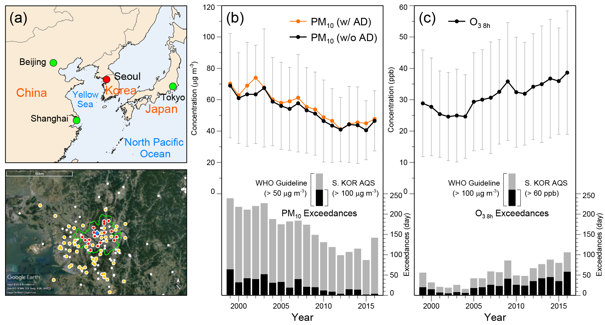
Figure 1 (a) Geographical locations of air quality monitoring sites in the SMA (circles) and the Seoul weather station (a blue solid diamond). Red solid circles denote 18 air quality monitoring sites utilized to obtain average daily air quality data in Seoul. Yellow solid circles show 52 air quality monitoring sites, which together with 18 sites (red solid circles) were used to calculate spatial gradients of the long-term components of air pollutants. Boundary of Seoul is marked with green line, and the satellite image is a courtesy of Google Earth Pro. Annual average concentrations and exceedances of the World Health Organization (WHO) guidelines and the South Korean AQS for (b) PM₁₀ (excluding AD days) and (c) O_3 8 h in Seoul. Annual average PM₁₀ concentrations including AD days are additionally represented as an orange line in (b). The vertical bars on the annual average concentrations indicate annual standard deviations.

The most noticeable features in the air pollutants data in Seoul are decreasing PM₁₀ and increasing O₃ levels on a long-term timescale. Annual average PM₁₀ concentrations and exceedance days of the South Korean air quality standard (AQS; 100 µg m⁻³) were decreased from 69 to 41 µg m⁻³ and from 64 to 2 days between 1999 and 2015 (Fig. 1b). Note that we excluded episodic Asian dust (AD) days (183 days for the analysis period; KMA, 2018a) from the PM₁₀ analysis to focus on the anthropogenic sources, although AD did not much affect the long-term PM₁₀ trend. On the other hand, annual average O_3 8 h levels and exceedance days of the AQS (60 ppbv) have been increased from 25 ppbv to 39 ppb and from 5 to 58 days between 2002 and 2016, respectively (Fig. 1c).

In terms of meteorological characteristics in Seoul, we used daily averages of temperature (^∘C), sea level pressure (hPa), relative humidity (%), wind speed (m s⁻¹), and solar irradiance (W m⁻²) at the Seoul weather station (Fig. 1a) managed by the Korea Meteorological Administration (KMA, 2018b). Note that the air quality monitoring sites in Seoul are spread over the area within a radius of ∼15 km from the weather station, and such spatial size is enough to resolve the influence of synoptic conditions on the local meteorological factors. To investigate the synoptic meteorological conditions, the geopotential height and wind fields at 850 hPa, 10 m wind fields, total cloud cover, and surface solar radiation were derived from the European Centre for Medium-Range Weather Forecasts Reanalysis Interim (ERA-Interim) data (Dee et al., 2011; http://apps.ecmwf.int/datasets/data/interim-full-daily/, last access: 31 October 2018).

We additionally employed estimated local emission data and several socioeconomic indices that could affect the emissions to compare with the separated emission-related air pollution trends. The annual estimated emissions of sulfur oxides (SO_x), NO_x, CO, volatile organic compounds (VOCs), and PM₁₀ in Seoul from the Clean Air Policy Support System (CAPSS) inventory (Lee et al., 2011; NIER, 2018); the national gross domestic product (GDP) growth (IMF, 2017); and the annual consumptions of the final energy, petroleum, and anthracite in Seoul (KEEI, 2016) were used in this study.

3 Decomposition of air pollutant time series

3.1 Temporal decomposition of air pollutant time series

The time series of daily air pollutant concentration at a given place comprises mainly three components: trend, seasonality, and white noise (Rao and Zurbenko, 1994). The trend (long-term component) is attributable to the long-term variations in local and regional emissions related to socioeconomic status and policies (Mijling et al., 2013) and the long-term changes in meteorological conditions, which can affect atmospheric chemistry and regional transport patterns (Cai et al., 2017; Zou et al., 2017). The seasonality (seasonal component) arises from the seasonal variations of meteorological conditions (Kim et al., 2018) and energy consumption pattern (Zhu et al., 2013). The white noise (short-term component) is a day-to-day variation mainly related to synoptic-scale weather changes, which control accumulation/ventilation of local air pollutants and transport of regional air pollutants (Seo et al., 2017), and is partly associated with short-term fluctuations in local emissions (Russell et al., 2010).

To decompose the air pollutant time series into these three components on different timescales, we used the KZ filter, which has been employed in many air pollution time series studies, particularly on O₃ and PM (Wise and Comrie, 2005; Seo et al., 2014; Ma et al., 2016; P. Li et al., 2017). The KZ filter, here denoted as KZ_(m, p), represents p times iteration of the moving average of time width m (days) and removes the high-frequency component of periods that are smaller than the effective filter width, N ($\ge m\times p^{\mathrm{1}/\mathrm{2}})$. The KZ filter method is applicable to the time series with missing data owing to the iterative moving average process and provides a high accuracy level comparable to that of the wavelet transform method, despite its simplicity (Eskridge et al., 1997). Here we applied KZ_(15, 5) and KZ_(365, 3) filters, which can remove variabilities of periods shorter than 33 days and 1.7 years, to filter out the short-term component and to leave the long-term component, respectively. The long-term component can be further separated into the emission-related trend and the meteorology-related trend by isolation of the emission-related component using a multiple-linear-regression model with representative meteorological variables.

Note that the original concentration (χ) was transformed into its natural logarithm values (X=lnχ) prior to the decomposition. Because the number distribution of daily air pollutant concentrations is usually lognormal (e.g., Fig. S2), the natural log transformation of the original concentration data is required for proper temporal decomposition with the KZ filter (Eskridge et al., 1997). The detailed decomposition procedure is described in the following and schematically summarized with PM₁₀ time series in Seoul in Fig. 2.

The time series of log-scaled pollutant concentration can be expressed as the sum of short-term (X_ST), seasonal (X_SN), and long-term (X_LT) components.

$$\begin{array}{}\text{(1)}& X\left(t\right)=X_{\mathrm{ST}}\left(t\right)+X_{\mathrm{SN}}\left(t\right)+X_{\mathrm{LT}}\left(t\right)\end{array}$$

The sum of seasonal and long-term components is a baseline $\left(X_{\mathrm{BL}}=X_{\mathrm{SN}}+X_{\mathrm{LT}}\right)$. X_BL and X_ST can be easily decomposed by applying the KZ_(15, 5) filter to X, which filters out the white-noise-like X_ST, as follows:

$$\begin{array}{}\text{(2)}& X_{\mathrm{BL}}\left(t\right)={\mathrm{KZ}}_{\left(\mathrm{15},\mathrm{5}\right)}\left[X\left(t\right)\right]=X\left(t\right)-X_{\mathrm{ST}}\left(t\right).\end{array}$$

Now the baseline can be assumed to consist of its repeated climatological seasonal cycle $\left(X_{\mathrm{BL}}^{\mathrm{clm}}\right)$ and residuals (ε).

$$\begin{array}{}\text{(3)}& X_{\mathrm{BL}}\left(t\right)=X_{\mathrm{BL}}^{\mathrm{clm}}\left(t\right)+\mathit{\epsilon }\left(t\right)\end{array}$$

Although $X_{\mathrm{BL}}^{\mathrm{clm}}$ obviously occupies most of the seasonality in X_BL, ε also contains some minor seasonal variability unconsidered in $X_{\mathrm{BL}}^{\mathrm{clm}}$ together with the long-term trend. To obtain the long-term component (X_LT) by filtering out the minor seasonality, the KZ_(365, 3) filter is applied to ε as follows:

$$\begin{array}{}\text{(4)}& X_{\mathrm{LT}}\left(t\right)={\mathrm{KZ}}_{\left(\mathrm{365},\mathrm{3}\right)}\left[\mathit{\epsilon }\left(t\right)\right]=X_{\mathrm{BL}}\left(t\right)-X_{\mathrm{SN}}\left(t\right).\end{array}$$

Then the seasonal component (X_SN), which represents the sum of the pure seasonal climatology $\left(X_{\mathrm{BL}}^{\mathrm{clm}}\right)$ and the minor seasonality ($\mathit{\epsilon }-{\mathrm{KZ}}_{\left(\mathrm{365},\mathrm{3}\right)}\left[\mathit{\epsilon }\right])$, can be obtained as the difference between X_BL and X_LT.

Note that, if we define χ_BL=exp(X_BL) and χ_ST=exp(X_ST) and employ the same concept to the relationship between the original concentration and its log transformation (χ=exp(X)), χ_BL represents the baseline concentration of the air pollutant and χ_ST becomes the ratio of original concentration to baseline concentration (χ∕χ_BL). Similarly, exp(X_SN) and exp(X_LT) can be defined as χ_SN and χ_LT, respectively. Then χ_SN represents the seasonal change in concentration without trend, and χ_LT becomes the ratio of baseline concentration to detrended seasonal concentration (χ_BL∕χ_SN).

As shown in the example with PM₁₀ in Seoul, the KZ_(15, 5) filter effectively removes ${\mathrm{PM}}_{{\mathrm{10}}_{\mathrm{ST}}}$ of periods shorter than 33 days and leaves both the seasonality of high PM₁₀ concentrations in winter and spring and the long-term decreasing trend in ${\mathrm{PM}}_{{\mathrm{10}}_{\mathrm{BL}}}$ (Figs. 2 and S4b). ${\mathrm{PM}}_{{\mathrm{10}}_{\mathrm{SN}}}$ and ${\mathrm{PM}}_{{\mathrm{10}}_{\mathrm{LT}}}$ represent well the seasonal variation, i.e., periods that are between 33 days and 1.7 years with representative periodicities of 0.5 and 1 years, and the long-term variations, i.e., periods that are longer than 1.7 years, respectively (Figs. 2 and S4c–d). The high levels in winter and spring of ${\mathrm{PM}}_{{\mathrm{10}}_{\mathrm{SN}}}$ in Seoul are attributable to the shallow boundary layer that traps local pollutants near the ground and frequent regional transport from China during the cold season (Kim et al., 2018).

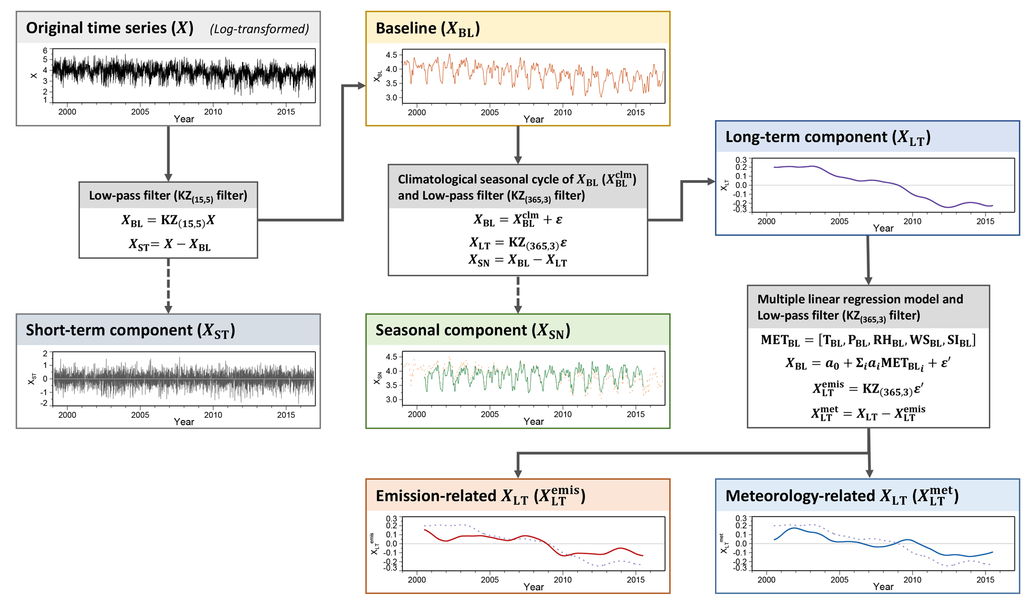
Figure 2 Schematic flowchart of temporal decomposition of air pollution time series (Seoul average daily PM₁₀ concentration) into short-term, seasonal, and emission-related and meteorology-related long-term components.

3.2 Separation of emission- and meteorology-related trends

Since the long-term variability in air pollutant concentrations can be affected not only by changes in local and regional emissions but also by changes in meteorological conditions, the long-term trend is assumed to consist of meteorologically adjusted (emission-related) long-term components $\left(X_{\mathrm{LT}}^{\mathrm{emis}}\right)$ and meteorology-related long-term components $\left(X_{\mathrm{LT}}^{\mathrm{met}}\right)$. Therefore, the baseline can be represented as follows:

$$\begin{array}{}\text{(5)}& X_{\mathrm{BL}}\left(t\right)=X_{\mathrm{SN}}\left(t\right)+X_{\mathrm{LT}}^{\mathrm{met}}\left(t\right)+X_{\mathrm{LT}}^{\mathrm{emis}}\left(t\right).\end{array}$$

To isolate the term $X_{\mathrm{LT}}^{\mathrm{emis}}$ in Eq. (5), we built a multiple-linear-regression model employing the baseline time series of the five representative meteorological variables (MET_BL), such as temperature (T_BL), sea level pressure (P_BL), relative humidity (RH_BL), wind speed (WS_BL), and solar irradiance (SI_BL), which are obtained by the KZ_(15, 5) filter as follows:

$$\begin{array}{ll}{\displaystyle }& {\displaystyle }{X}_{\mathrm{BL}}\left(t\right)=a_{\mathrm{0}}+{\sum }_i{a}_i{\mathrm{MET}}_{{\mathrm{BL}}_i}\left(t\right)+\mathit{\epsilon }{}^{\prime }\left(t\right),\\ \text{(6)}& {\displaystyle }& {\displaystyle }{\mathrm{MET}}_{\mathrm{BL}}=\left[T_{\mathrm{BL}},P_{\mathrm{BL}},{\mathrm{RH}}_{\mathrm{BL}},{\mathrm{WS}}_{\mathrm{BL}},{\mathrm{SI}}_{\mathrm{BL}}\right],\end{array}$$

where ε^′ is the sum of the non-meteorological long-term variability $\left(X_{\mathrm{LT}}^{\mathrm{emis}}\right)$ and the minor seasonal variability unexplained by the multiple-linear-regression model $\left({\mathit{\epsilon }}^{\prime }-X_{\mathrm{LT}}^{\mathrm{emis}}\right)$. Note that daily maximum temperature ($T_{{\max }_{\mathrm{BL}}}$) was used for the model of O${}_{\mathrm{3}\mathrm{8}{\mathrm{h}}_{\mathrm{BL}}}$ instead of daily average temperature (T_BL) considering daytime O₃ as in a previous study (Seo et al., 2014). By removing the minor seasonality from ε^′ using the KZ_(365, 3) filter, $X_{\mathrm{LT}}^{\mathrm{emis}}$ can be isolated as follows:

$$\begin{array}{}\text{(7)}& X_{\mathrm{LT}}^{\mathrm{emis}}\left(t\right)={\mathrm{KZ}}_{\left(\mathrm{365},\mathrm{3}\right)}\left[{\mathit{\epsilon }}^{\prime }\left(t\right)\right]=X_{\mathrm{LT}}\left(t\right)-X_{\mathrm{LT}}^{\mathrm{met}}\left(t\right).\end{array}$$

Then $X_{\mathrm{LT}}^{\mathrm{met}}$ can be simply obtained by differencing between X_LT and $X_{\mathrm{LT}}^{\mathrm{emis}}$.

In the example displayed in Fig. 2, ${\mathrm{PM}}_{{\mathrm{10}}_{\mathrm{LT}}}$ in Seoul shows a continuous decrease between 2003 and 2012. Such a decreasing trend in PM₁₀ has been recognized as a result of the reduction in diesel vehicle emissions and fugitive dust in Seoul (Ghim et al., 2015; Kim and Lee, 2018). However, a recent modeling study suggested that the long-term increase in wind speed might additionally contribute to the past improvement of PM₁₀ air quality in Seoul (Kim et al., 2017). In fact, both ${\mathrm{PM}}_{{\mathrm{10}}_{\mathrm{LT}}}^{\mathrm{emis}}$ and ${\mathrm{PM}}_{{\mathrm{10}}_{\mathrm{LT}}}^{\mathrm{met}}$ in Fig. 2 show decreasing patterns, and this supports probable influences of both emission controls and meteorology on the PM₁₀ trend in Seoul.

3.3 Contributions of local emissions and transport to the long-term trends

$X_{\mathrm{LT}}^{\mathrm{emis}}$ contains both changes in local emissions $\left(X_{\mathrm{LT}}^{\mathrm{emis}\left(\mathrm{L}\right)}\right)$ and changes in transport of regional emissions $\left(X_{\mathrm{LT}}^{\mathrm{emis}\left(\mathrm{T}\right)}\right)$, and thus X_LT can be represented as Eq. (8).

$$\begin{array}{}\text{(8)}& X_{\mathrm{LT}}\left(t\right)=X_{\mathrm{LT}}^{\mathrm{emis}\left(T\right)}\left(t\right)+X_{\mathrm{LT}}^{\mathrm{emis}\left(\mathrm{L}\right)}\left(t\right)+X_{\mathrm{LT}}^{\mathrm{met}}\left(t\right)\end{array}$$

Then the rate of change of X_LT should satisfy a simple continuity equation as follows:

$$\begin{array}{}\text{(9)}& {\displaystyle \frac{\partial X_{\mathrm{LT}}}{\partial t}}=-{\mathit{V}}_{\mathrm{LT}}\cdot \mathrm{\nabla }{X}_{\mathrm{LT}}+S_{\mathrm{LT}},\end{array}$$

where the advection term, $-{\mathit{V}}_{\mathrm{LT}}\cdot \mathrm{\nabla }{X}_{\mathrm{LT}}$, represents the transport of regional emissions mainly by horizontal winds, and the sources and sinks term, S_LT, can be regarded as the long-term changes by both local emissions and chemical production, accumulation, and dissipation by meteorological factors. Because X_LT and $X_{\mathrm{LT}}^{\mathrm{met}}$ were already known, the rates of change of $X_{\mathrm{LT}}^{\mathrm{emis}\left(\mathrm{T}\right)}$ and $X_{\mathrm{LT}}^{\mathrm{emis}\left(\mathrm{L}\right)}$ can be derived as follows (see Sect. S1 in the Supplement):

$$\begin{array}{ll}{\displaystyle }& {\displaystyle \frac{\partial }{\partial t}}\left(X_{\mathrm{LT}}^{\mathrm{emis}\left(\mathrm{T}\right)}\right)=-{\mathit{V}}_{\mathrm{LT}}\cdot \mathrm{\nabla }{X}_{\mathrm{LT}}=-u_{\mathrm{LT}}\left({\displaystyle \frac{\partial X_{\mathrm{BL}}}{\partial x}}-{\displaystyle \frac{\partial X_{\mathrm{SN}}}{\partial x}}\right)\\ \text{(10)}& {\displaystyle }& {\displaystyle }-v_{\mathrm{LT}}\left({\displaystyle \frac{\partial X_{\mathrm{BL}}}{\partial y}}-{\displaystyle \frac{\partial X_{\mathrm{SN}}}{\partial y}}\right),\text{(11)}& {\displaystyle }& {\displaystyle \frac{\partial }{\partial t}}\left(X_{\mathrm{LT}}^{\mathrm{emis}\left(\mathrm{L}\right)}\right)={\displaystyle \frac{\partial X_{\mathrm{LT}}}{\partial t}}-\left[{\displaystyle \frac{\partial X_{\mathrm{LT}}^{\mathrm{met}}}{\partial t}}+{\displaystyle \frac{\partial }{\partial t}}\left(X_{\mathrm{LT}}^{\mathrm{emis}\left(\mathrm{T}\right)}\right)\right],\end{array}$$

where ${\mathit{V}}_{\mathrm{LT}}=\left(u_{\mathrm{LT}},v_{\mathrm{LT}}\right)$ is long-term zonal and meridional winds components representative for the target area, and ∇X_LT is the horizontal gradient of long-term components of air pollution for the larger area, which are identical to the difference between ∇X_BL and ∇X_SN. If ∇X_LT>0 at a specific time, then the horizontal gradient of baseline (∇X_BL) at that time is steeper than that of seasonal climatology (∇X_SN). Note that the above method for evaluating the changes in $X_{\mathrm{LT}}^{\mathrm{emis}\left(\mathrm{T}\right)}$ and $X_{\mathrm{LT}}^{\mathrm{emis}\left(\mathrm{L}\right)}$ is applicable not to data from the individual site but to data from the wider area, because of the requirement of the horizontal gradient term in Eq. (10).

In this study, we choose 70 air quality monitoring sites over the SMA, which are spread over the area within a radius of 50 km from the Seoul weather station, based on data availability of more than 75 % for 1999–2016 (Fig. 1a). Daily X_BL and X_SN at those sites were utilized to determine ∇X_BL and ∇X_SN by linear regressions of X_BL and X_SN on the zonal and meridional distances from the weather station and finally to obtain ∇X_LT ($=\mathrm{\nabla }{X}_{\mathrm{BL}}-\mathrm{\nabla }{X}_{\mathrm{SN}}$; Figs. S5 and S6c, e, g, i, and k). Also, u_LT and v_LT in Seoul are calculated by the KZ_(365, 3) filter with wind direction and speed at the Seoul weather station (Fig. S6a and b). From V_LT and ∇X_LT of each species, we calculated the long-term transport terms for each air pollutant species in Seoul (Fig. S6d, f, h, j, and l).

Figure 3 Lag composites of seasonal anomalies of geopotential height (contours with interval of 2.5 gpm) and wind (arrows with reference scale of 1 m s⁻¹) at 850 hPa relative to each first day that $\exp \left({\mathrm{PM}}_{{\mathrm{10}}_{\mathrm{ST}}}\right)$ exceeds the sum of its mean and 1 standard deviation. Total number of events, mean, and standard deviation is 283, 1, and 0.50, respectively. Geopotential height and wind statistically significant at the 95% confidence level are represented as light gray shading and arrows. Location of Seoul is marked by solid red circles.

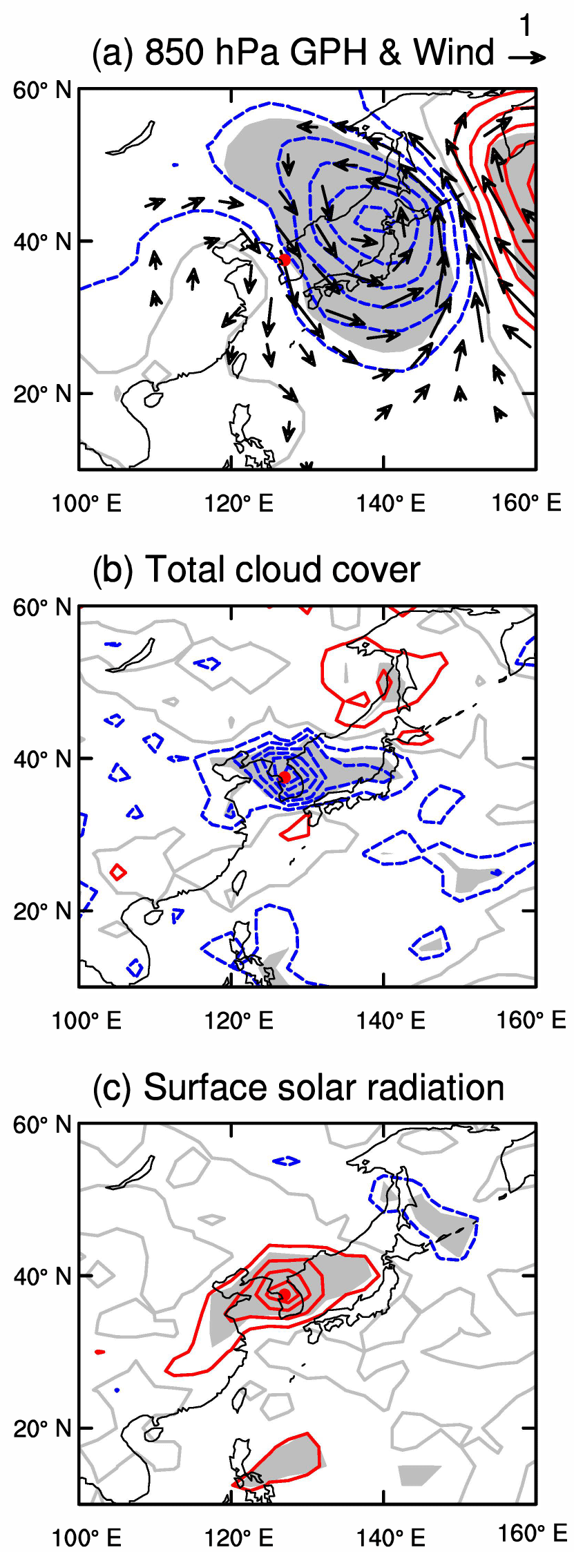
Figure 4 Composites of seasonal anomalies of (a) geopotential height (contours with interval of 2.5 gpm) and wind (arrows with reference scale of 1 m s⁻¹) at 850 hPa, (b) total cloud cover fraction (contours with interval of 2 %), (c) downward solar radiation anomaly at the surface (contours with interval of 5 W m⁻²) for each first day that $\exp \left({\mathrm{O}}_{\mathrm{3}\mathrm{8}{\mathrm{h}}_{\mathrm{ST}}}\right)$ exceeds the sum of the mean and 1 standard deviation. Total number of events, mean, and standard deviation is 346, 1, and 0.41, respectively. Geopotential height and wind, total cloud cover, and downward solar radiation statistically significant at the 95 % confidence level are represented by light gray shading and arrows. Location of Seoul is marked by a solid red circle.

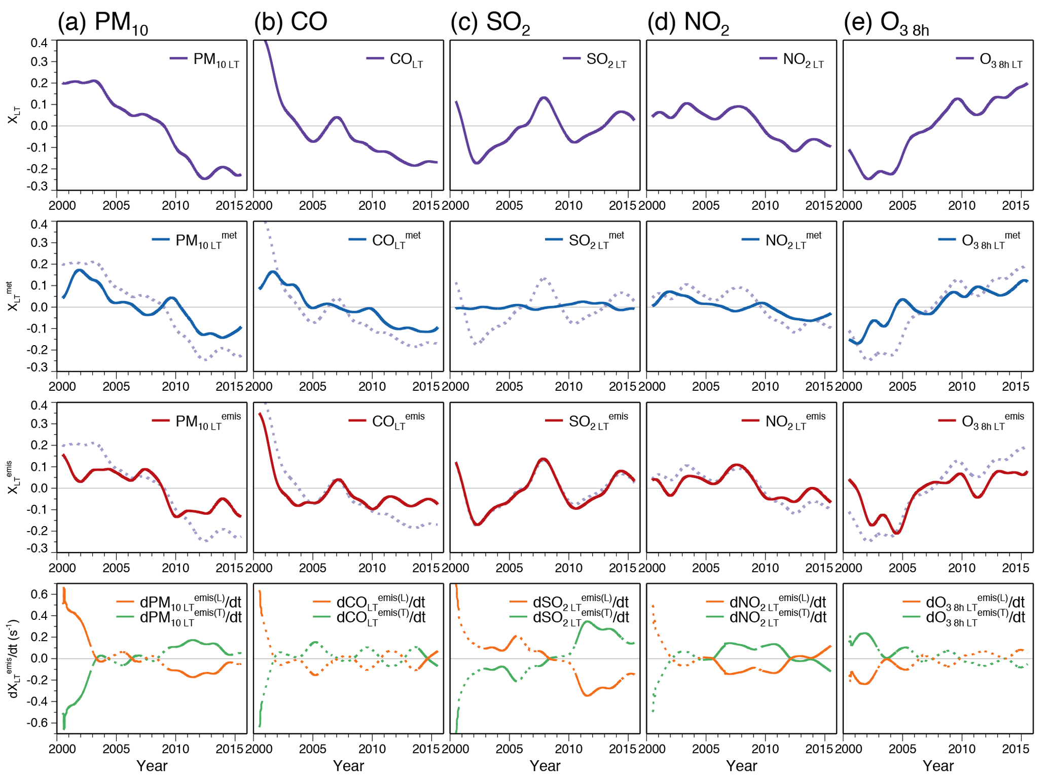
Figure 5 Long-term components that are unadjusted for meteorological variables (X_LT; violet lines), meteorology-related $\left(X_{\mathrm{LT}}^{\mathrm{met}};\mathrm{blue}\mathrm{lines}\right)$ and emission-related $\left(X_{\mathrm{LT}}^{\mathrm{emis}};\mathrm{redlines}\right)$ long-term components, and contributions of local emissions $\left(\frac{\partial }{\partial t}{X}_{\mathrm{LT}}^{\mathrm{emis}\left(\mathrm{L}\right)};\mathrm{orange}\mathrm{lines}\right)$ and transport of regional emissions $\left(\frac{\partial }{\partial t}{X}_{\mathrm{LT}}^{\mathrm{emis}\left(\mathrm{T}\right)};\mathrm{green}\mathrm{lines}\right)$ to the long-term trends of (a) PM₁₀, (b) CO, (c) SO₂, (d) NO₂, and (e) O_3 8 h in Seoul. Solid lines in $\frac{\partial }{\partial t}{X}_{\mathrm{LT}}^{\mathrm{emis}\left(\mathrm{L}\right)}$ and $\frac{\partial }{\partial t}{X}_{\mathrm{LT}}^{\mathrm{emis}\left(\mathrm{T}\right)}$ show that the horizontal gradients of X_LT (∇X_LT) obtained by linear regression are statistically significant at the 95 % level or higher (p < 0.05).

In Eq. (11), $\frac{\partial X_{\mathrm{LT}}}{\partial t}$ and $\frac{\partial X_{\mathrm{LT}}^{\mathrm{met}}}{\partial t}$ are 3 orders of magnitude smaller than $\frac{\partial }{\partial t}\left(X_{\mathrm{LT}}^{\mathrm{emis}\left(\mathrm{L}\right)}\right)$ and $\frac{\partial }{\partial t}\left(X_{\mathrm{LT}}^{\mathrm{emis}\left(\mathrm{T}\right)}\right)$, and thus approximately $\frac{\partial }{\partial t}\left(X_{\mathrm{LT}}^{\mathrm{emis}\left(\mathrm{L}\right)}\right)\approx -\frac{\partial }{\partial t}\left(X_{\mathrm{LT}}^{\mathrm{emis}\left(\mathrm{T}\right)}\right)$. For example, if we assume that χ∼50 µg m⁻³, $\frac{\partial \mathit{\chi }}{\partial t}$ $\sim -\mathrm{10}$ µg m⁻³ decade⁻¹, $\frac{\partial \mathit{\chi }}{\partial x}\sim -\mathrm{10}$ µg m⁻³ (100 km)⁻¹, and u∼1 m s⁻¹ at a given place at which conditions are similar to PM₁₀ levels in Seoul and its metropolitan area, then the transport term $-u\frac{\partial X}{\partial x}\left(=-\frac{u}{\mathit{\chi }}\frac{\partial \mathit{\chi }}{\partial x}\right)$ $\sim -\mathrm{2}\times {\mathrm{10}}^{-\mathrm{6}}$ s⁻¹, while the tendency term $\frac{\partial X}{\partial t}$ $\left(=\frac{\mathrm{1}}{\mathit{\chi }}\frac{\partial \mathit{\chi }}{\partial t}\right)$ $\sim -\mathrm{2.5}\times {\mathrm{10}}^{-\mathrm{9}}$ s⁻¹. If we further assume that the local PM₁₀ emission in Seoul (area of 605 km²) has the same order of magnitude as the transport term for the concentration $\left(u\frac{\partial \mathit{\chi }}{\partial x}\sim \mathrm{1}\times {\mathrm{10}}^{-\mathrm{4}}\mathrm{\mu }\mathrm{g}{\mathrm{m}}^{-\mathrm{3}}{\mathrm{s}}^{-\mathrm{1}}\right)$ and the boundary layer height over the area is about 1 km, the total amount of yearly PM₁₀ emission in Seoul will be approximately 1.9 kt, which is consistent with the estimation by the CAPSS emission inventory (Fig. 5a; NIER, 2018). In fact, because air pollutant concentrations are close to the steady state for the long-term period, its tendency is a small residual between two large terms: influx of clean or polluted air (transport) and local emissions/production or dissipation/deposition (sources and sinks). It should be noted that the transport term and the source/sink term, however, are not balanced against each other on a short-term timescale because the day-to-day rate of change of the air pollution concentration is comparable to both transport and source/sink terms.

4 Application to air pollutants in Seoul

Variances of each timescale component of PM₁₀, SO₂, NO₂, and CO in Seoul were generally largest in the short-term fluctuation (∼46–68 %), while that of O_3 8 h was largest in its seasonal cycle (Table 1). This indicates an important role of synoptic-scale weather on the day-to-day variations of the primary air pollutants concentrations in Seoul. The changes in synoptic flow pattern control local air quality by accumulation/ventilation and regional transport of air pollutants (Zheng et al., 2015; Seo et al., 2017). On the other hand, O₃ is a photochemical product and thus is controlled largely by the annual cycle of solar irradiance in such a NO_x- and VOC-rich urban area, although its short-term variability, which is caused by the changes in synoptic weather and related precursor concentrations and irradiance, is comparable to the seasonal variability.

Table 1 Total variances (Var(X)) of log-scale times series for Seoul average concentrations of PM₁₀, SO₂, NO₂, CO, and O_3 8 h, and relative contributions (%) of variances of and covariances (Cov) among each component to Var(X). Daily data for the period of July 2000 to June 2015 during which X_LT data are available were used.

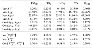
^* Values of variances of each pollutant time series Var$\left(X\right)=\mathrm{Var}\left(X_{\mathrm{ST}}\right)+\mathrm{Var}\left(X_{\mathrm{ST}}\right)+\mathrm{Var}\left(X_{\mathrm{ST}}\right)+\mathrm{2}\left[\mathrm{Cov}\left(X_{\mathrm{ST}},X_{\mathrm{SN}}\right)+\mathrm{Cov}\left(X_{\mathrm{SN}},X_{\mathrm{LT}}\right)+\mathrm{Cov}\left(X_{\mathrm{ST}},X_{\mathrm{LT}}\right)\right]$

In terms of the long-term trends, variabilities related to the long-term local and regional emission changes $\left(X_{\mathrm{LT}}^{\mathrm{emis}}\right)$ are comparable to those induced by the long-term meteorological effects $\left(X_{\mathrm{LT}}^{\mathrm{met}}\right)$ for PM₁₀, NO₂, CO, and O_3 8 h, while $X_{\mathrm{LT}}^{\mathrm{emis}}$ is dominant for total long-term variabilities of SO₂ (Table 1). Since the local-scale meteorology could affect more the local emission-related long-term trend rather than the regional background-related long-term trend, the smaller variability of $X_{\mathrm{LT}}^{\mathrm{met}}$ implies a smaller influence of the local emission changes compared to the regional background level changes on $X_{\mathrm{LT}}^{\mathrm{emis}}$.

4.1 Meteorological effects on seasonality in air pollution

In the process of isolating $X_{\mathrm{LT}}^{\mathrm{emis}}$ from X_LT, the multiple-linear-regression model predicting X_BL from meteorological predictors (MET_BL) was used. The model using the meteorological variables explains well O${}_{\mathrm{3}\mathrm{8}{\mathrm{h}}_{\mathrm{BL}}}$ (adjusted R²=0.86), while the baseline of PM₁₀ (${\mathrm{PM}}_{{\mathrm{10}}_{\mathrm{BL}}}$) is much less explained by the model (adjusted R²=0.51; Table 2). This indicates that the long-term non-meteorological (or emission-related) variability in ${\mathrm{PM}}_{{\mathrm{10}}_{\mathrm{BL}}}$ is much larger than that in O${}_{\mathrm{3}\mathrm{8}{\mathrm{h}}_{\mathrm{BL}}}$. In the linear regression model, ${\mathrm{PM}}_{{\mathrm{10}}_{\mathrm{BL}}}$ and the baselines of primary gaseous pollutants of SO₂, NO₂, and CO commonly show strong positive correlation with P_BL but strong negative correlations with T_BL and RH_BL, while O${}_{\mathrm{3}\mathrm{8}{\mathrm{h}}_{\mathrm{BL}}}$ shows strong positive correlations (p < 0.05) with SI_BL and $T_{{\max }_{\mathrm{BL}}}$ but strong negative correlation (p < 0.05) with P_BL (Table 2). Meteorological conditions over the Korean Peninsula in winter are affected by a cold and dry Siberian high that causes both the shallow boundary layer to trap the primary air pollutants near the surface and the northwesterly winds to transport the regional pollutants from the continent (Kim et al., 2018) and thus elevates ${\mathrm{PM}}_{{\mathrm{10}}_{\mathrm{BL}}}$ in winter to early spring (Fig. S3b). On the other hand, enhanced photochemistry by strong irradiance together with temperature effects on O₃ formation (increasing of biogenic hydrocarbons and hydroxyl radicals and enhanced thermal decomposition of peroxyacetyl nitrate in warm conditions; e.g., Sillman and Samson, 1995) elevates O_3 8 h levels in late spring and summer in Seoul (Fig. S3b).

Table 2 Correlation coefficients (r) between baseline time series of pollutants (PM₁₀, SO₂, NO₂, CO, and O_3 8 h) and meteorological variables (T, T_max, P, RH, WS, and SI), and adjusted R² between the baseline time series of pollutants (X_BL) and multiple-linear-regression model ($a_{\mathrm{0}}+{\sum }_i{a}_i{\mathrm{MET}}_{{\mathrm{BL}}_i}$).

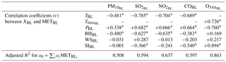
^* The correlation is statistically significant at the 95 % level or higher (p < 0.05).

4.2 Synoptic influences on short-term air pollution events

The short-term air pollution variability is closely related to the day-to-day variations of local meteorological factors. Intercorrelations among X_ST of air pollutant species and meteorological variables in Seoul are summarized in Table 3. Note that using X_ST instead of the original daily concentrations has the advantage of providing short-term features unbiased to seasonal characteristics and background levels because exp(X_ST) is equivalent to the ratio of measured concentration to filtered baseline concentration as aforementioned in Sect. 3.1.

Table 3 Correlation coefficients (r) among short-term components of each pollutant and meteorological variable in Seoul for the period between February 1999 and November 2016.

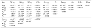
^* The correlation is statistically significant at the 99 % level or higher (p < 0.01).

Significant positive intercorrelations (p < 0.01) among ${\mathrm{PM}}_{{\mathrm{10}}_{\mathrm{ST}}}$ and primary gaseous pollutants (SO${}_{{\mathrm{2}}_{\mathrm{ST}}}$, NO${}_{{\mathrm{2}}_{\mathrm{ST}}}$, and CO_ST) together with their strong negative relationships to T_ST and WS_ST (p < 0.01) indicate that the high-PM₁₀ episodes in Seoul occurred in warm and stagnant weather conditions. Such warm and stagnant conditions can be induced by the migratory high-pressure system (e.g., negative relationships of WS_ST to T_ST and P_ST in Table 3) or by the warm front of the extratropical cyclone (e.g., negative correlations of T_ST to WS_ST and P_ST but its positive correlation to RH_ST in Table 3). The lag composites of the geopotential height and wind anomalies at 850 hPa (about 1.5 km altitude) relative to each day of $\exp \left({\mathrm{PM}}_{{\mathrm{10}}_{\mathrm{ST}}}\right)$, which is equivalent to the ratios of measured concentration to the filtered baseline concentration of PM₁₀, exceeding the sum of its mean and 1 standard deviation (> 1.50) indicate that the high-PM₁₀ episodes in Seoul are associated with the former conditions (Fig. 3). As shown in Fig. 3a–c, a high-pressure anomaly develops over southern China and moves eastward in 3 days before the high-PM₁₀ days. This kind of synoptic pattern can induce both slow regional transport of secondary precursors from China along the northern boundary of the high-pressure system (Fig. 3b and c) and gradual accumulation of primary and secondary aerosols in a local area in the high-pressure system (Fig. 3d; Seo et al., 2017). Strong correlations of ${\mathrm{PM}}_{{\mathrm{10}}_{\mathrm{ST}}}$ with SO${}_{{\mathrm{2}}_{\mathrm{ST}}}$ and NO${}_{{\mathrm{2}}_{\mathrm{ST}}}$ (p < 0.01; Table 3) imply possible large contributions of secondary species such as sulfate and nitrate aerosols to the haze episodes in Seoul. In fact, previous studies have reported that the proportion of secondary inorganic aerosols to fine-mode PM (PM_2.5) was measured as high as ∼50 % on average and even reached ∼75 % during the severe-haze event (Seo et al., 2017; Kim et al., 2018).

Table 4 Linear trends of long-term components of air pollutants and meteorological variables in Seoul for the period between July 2000 and June 2015.

^* The slope of linear trend is statistically significant at the 90 % level or higher (p < 0.1).

In terms of short-term variability in O_3 8 h levels in Seoul, O${}_{\mathrm{3}\mathrm{8}{\mathrm{h}}_{\mathrm{ST}}}$ is strongly correlated positively with SI_ST and $T_{{\max }_{\mathrm{ST}}}$ but negatively with RH_ST (p < 0.01; Table 3). This likely reflects favorable meteorological environment for O₃ formation: strong irradiance with warm and dry conditions. Interestingly, O${}_{\mathrm{3}\mathrm{8}{\mathrm{h}}_{\mathrm{ST}}}$ shows positive correlation with WS_ST, although stagnant conditions are regarded as conducive to O₃ formation in general. This is related to the strong negative relationship between O${}_{\mathrm{3}\mathrm{8}{\mathrm{h}}_{\mathrm{ST}}}$ and NO${}_{{\mathrm{2}}_{\mathrm{ST}}}$ and that between WS_ST and NO${}_{{\mathrm{2}}_{\mathrm{ST}}}$. Since the reaction with NO, which is produced by photolysis of NO₂, is a major sink of O₃, high NO₂ concentration reduces O₃ on high-irradiance days, while the low NO₂ concentration can increase O₃. In addition, NO${}_{{\mathrm{2}}_{\mathrm{ST}}}$ and CO_ST are strongly correlated ($r=+\mathrm{0.86}$) because both CO and NO_x are mainly emitted by transportation exhaust in Seoul (82 % of CO and 67 % of NO_x emissions; NIER, 2018), and thus O${}_{\mathrm{3}\mathrm{8}{\mathrm{h}}_{\mathrm{ST}}}$ has a negative relationship with CO_ST, similar to that with NO${}_{{\mathrm{2}}_{\mathrm{ST}}}$. The composites of the 850 hPa geopotential height and wind anomalies for high-O_3 8 h days that $\exp \left({\mathrm{O}}_{\mathrm{3}\mathrm{8}{\mathrm{h}}_{\mathrm{ST}}}\right)$ exceeds the sum of its mean and 1 standard deviation (> 1.41) show that the high-O_3 8 h event frequently occurs at the transition of weather from the cyclonic anomaly to the anticyclonic anomaly (Fig. 4a). As the anomalous low-pressure system moves eastward out of the Korean Peninsula, the decrease in cloud cover (Fig. 4b) results in the increase in surface irradiance (Fig. 4c) and thus the O₃ level. Since this kind of anomalous synoptic pattern enhances the mean westerly flow by the anomalous northwesterly (Figs. 4a and S7a), the wind speed in this region is increased. As shown by the strong positive correlations between WS_ST and NO${}_{{\mathrm{2}}_{\mathrm{ST}}}$ (Table 3), NO₂ can be reduced by the high winds and thus could contribute to the high O₃ concentration on short-term timescales.

4.3 Long-term trends of air pollution in Seoul

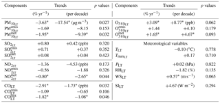
Times series of X_LT and its two decomposed components, $X_{\mathrm{LT}}^{\mathrm{emis}}$ and $X_{\mathrm{LT}}^{\mathrm{met}}$, for each air pollutant species are shown in Fig. 5, and their linear trends are summarized in Table 4. Note that these time series range from July 2000 to June 2015 because 546 days at the beginning and ending of data were lost due to the truncation effect of the KZ_(365, 3) filter. The linear trend of X_LT represents a fractional change rate (% yr⁻¹) of the baseline concentration (χ_BL) because $\frac{\partial X_{\mathrm{LT}}}{\partial t}$ is equivalent to $\frac{\mathrm{1}}{{\mathit{\chi }}_{\mathrm{BL}}}\frac{\partial {\mathit{\chi }}_{\mathrm{BL}}}{\partial \mathrm{t}}$. The fractional change rate can be converted into an equivalent concentration change rate by multiplying with temporal-mean χ_BL for the analysis period.

In Seoul, there are significant decreasing trends (p < 0.05) in ${\mathrm{PM}}_{{\mathrm{10}}_{\mathrm{LT}}}$ (−3.6 % yr⁻¹) and CO_LT (−2.9 % yr⁻¹) and an increasing trend (p < 0.1) in O${}_{\mathrm{3}\mathrm{8}{\mathrm{h}}_{\mathrm{LT}}}$ (+3.1 % yr⁻¹) for the last 15 years, while NO${}_{{\mathrm{2}}_{\mathrm{LT}}}$ (−1.4 % yr⁻¹) and SO${}_{{\mathrm{2}}_{\mathrm{LT}}}$ (+0.8 % yr⁻¹) do not show statistically significant trends (Table 4). The decrease of PM₁₀ concentration and increase of O_3 8 h level in their long-term linear trends can be clearly identified in temporal variation of X_LT (Fig. 3a and e) and are consistent with the temporal characteristics in their annual average concentrations (Fig. 1b and c). In terms of CO, abrupt decrease in the early 2000s, which was reported to be associated with introduction of natural gas vehicle supply and improvement of fuel quality (Kim and Shon, 2011), affects such a strong linear trend (Fig. 5b). On the other hand, SO₂ concentration in Seoul already stabilized at ∼5 ppb during the last decade (Fig. 5c), although it decreased significantly in the 1980s and 1990s owing to the government's efforts to control the SO_x emissions by use of low-sulfur fuel and natural gas for industry and transportation (Ray and Kim, 2014; NIER, 2017). NO₂ concentration varied between 30 and 40 ppb in the last decade and also shows a relatively weak trend (Fig. 5d; NIER, 2017). Interestingly, the NO₂ level has stabilized despite an increase of the number of vehicles in Seoul from 2.3 million in 1999 to 3.1 million in 2016 probably owing to implementation of natural gas vehicles and low-emission diesel engines, and the NO_x (= NO+NO₂) level has even decreased from ∼70 to ∼50 ppb for the same period (Shon and Kim, 2011; Kim and Lee, 2018). Such an increase of NO₂ to NO_x ratio implies that additional conversion of the NO-to-NO₂ occurs somewhere before the emission (e.g., exhaust line of the vehicle) or in the atmosphere. Although further evidence is required, this could be attributable to the expansion of diesel particulate filter (DPF) and diesel oxidation catalyst (DOC) usage for diesel vehicles or the increase of atmospheric oxidative potential in the SMA (Alvarez et al., 2008; Kim and Lee, 2018). Since Seoul is a NO_x-saturated regime area (Jin et al., 2012), such a decreasing trend in ambient NO_x concentration in recent decades may be one of the causes of the long-term increase of O_3 8 h in Seoul.

Although the decreasing trends in ${\mathrm{PM}}_{{\mathrm{10}}_{\mathrm{LT}}}$, CO_LT, and NO${}_{{\mathrm{2}}_{\mathrm{LT}}}$ in the last decade have been regarded as the result of efforts to reduce the local emissions (Kim and Lee, 2018), their $X_{\mathrm{LT}}^{\mathrm{emis}}$ linear trends are less than half of X_LT linear trends (Table 4). This indicates the more important role of the long-term changes in local meteorology in the long-term air pollution trends in Seoul.

In contrast to the comparable linear trends of $X_{\mathrm{LT}}^{\mathrm{emis}}$ and $X_{\mathrm{LT}}^{\mathrm{met}}$ of PM₁₀, CO, and NO₂, the linear trend of SO${}_{{\mathrm{2}}_{\mathrm{LT}}}$ is dominantly contributed by that of SO${}_{{\mathrm{2}}_{\mathrm{LT}}}^{\mathrm{emis}}$ (Table 4). This suggests a larger influence of the regional background SO₂ than that of the local SO_x emission on SO${}_{{\mathrm{2}}_{\mathrm{LT}}}^{\mathrm{emis}}$ because the long-term effects of local meteorological conditions on the local emission-related air pollution trend must be limited if the long-term change in local emission is negligible. In fact, the estimated SO_x emission intensity of Seoul (7.4 t km⁻²) in the reference year 2010 was much lower than that of an industrial port city in the west adjacent to Seoul, Incheon (18.1 t km⁻²), or the Chinese eastern coastal region of Jing-Jin-Ji (Beijing–Tianjin–Hebei), Shandong, Jiangsu, and Shanghai (14.3 t km⁻²; M. Li et al., 2017; NIER, 2018). In consideration of the prevailing westerlies in this region (Fig. S7a), the long-term SO₂ concentration trend in Seoul could be more affected by the long-term change in regional background level than by that in local emission.

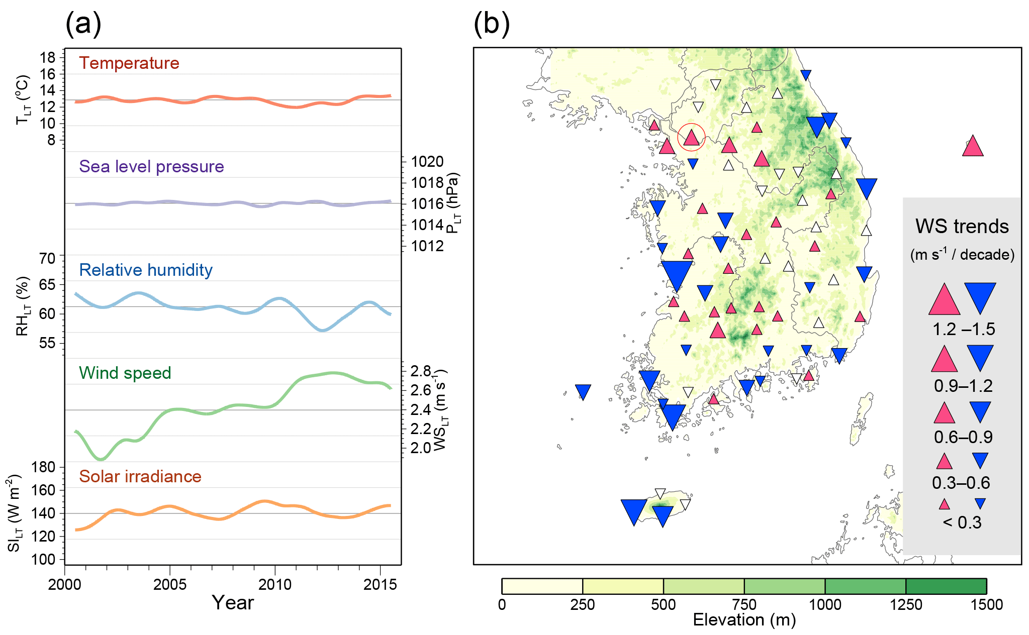
Figure 6 (a) Long-term components of daily average temperature, sea level pressure, relative humidity, wind speed, and solar irradiance. Vertical scales represented by gray horizontal lines are equivalent to 0.3 standard deviation of each original time series of the meteorological variables. (b) Linear trends of wind speed observed at 75 weather stations over South Korea for the period of 1999–2016. Upward and downward triangles with colors indicate the increasing and decreasing trends which are statistically significant at or above the 95 % confidence level (p < 0.05), respectively. Location of Seoul is marked by a red open circle.

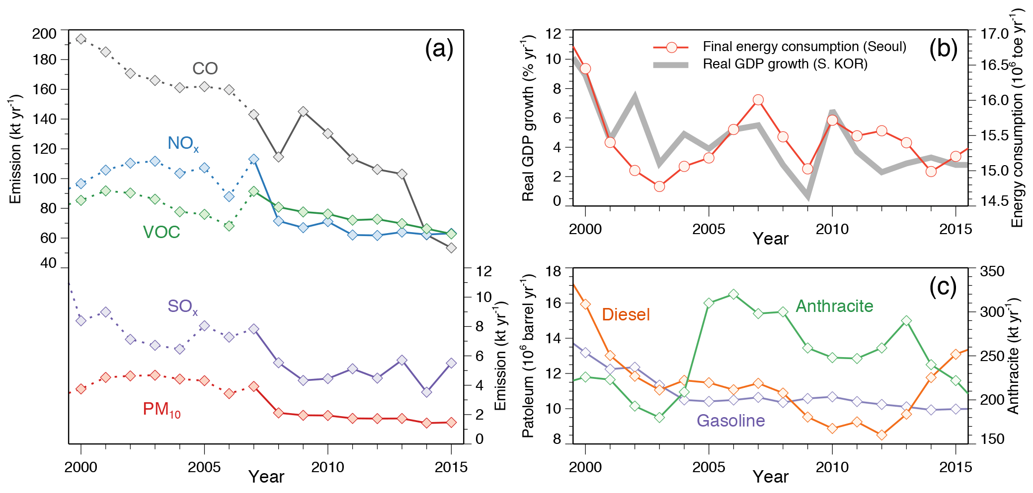
Figure 7 (a) Annual emissions of SO_x, NO_x, CO, VOCs, and PM₁₀ in Seoul. Note that the estimation method for the CAPSS inventory has been continuously updated, but the significant update was made in the year 2007. Emissions before and after 2007 were distinguished by dotted and solid lines. (b) Final energy consumption in Seoul and real GDP growth of South Korea. (c) Diesel, gasoline, and anthracite consumptions in Seoul.

In the reference year 2010, emission intensities of CO and NO_x in Seoul in 2010 were estimated as 215.3 t km⁻² and 117.4, respectively, and these are obviously much higher than those in Incheon (44.1 t km⁻² for CO and 51.3 t km⁻² for NO_x) or the Chinese eastern coastal region (98.1 t km⁻² for CO and 17.4 t km⁻² for NO_x; M. Li et al., 2017; NIER, 2018). Therefore, CO${}_{\mathrm{LT}}^{\mathrm{emis}}$ and NO${}_{{\mathrm{2}}_{\mathrm{LT}}}^{\mathrm{emis}}$ in Seoul are probably much more affected by the long-term changes in local emissions than by the changes in regional background levels.

4.3.1 Meteorology-related long-term trends

For most of the species in Seoul except SO₂, larger decreasing trends of $X_{\mathrm{LT}}^{\mathrm{met}}$ than of $X_{\mathrm{LT}}^{\mathrm{emis}}$ have been found (Table 4). For example, the equivalent linear trend of ${\mathrm{PM}}_{{\mathrm{10}}_{\mathrm{LT}}}$ was −17.5 µg m⁻³ decade⁻¹, while that of ${\mathrm{PM}}_{{\mathrm{10}}_{\mathrm{LT}}}^{\mathrm{emis}}$ was only −8.1 µg m⁻³ decade⁻¹. Thus, the recent achievement of ambient PM₁₀ reduction in Seoul would be less successful without the contribution by the ${\mathrm{PM}}_{{\mathrm{10}}_{\mathrm{LT}}}^{\mathrm{met}}$ trend (−9.4 µg m⁻³ decade⁻¹; Table 4 and Fig. 5a). In terms of O₃, the equivalent linear trend of O${}_{\mathrm{3}\mathrm{8}{\mathrm{h}}_{\mathrm{LT}}}$ (+8.8 ppb decade⁻¹) was also contributed to slightly more by O${}_{\mathrm{3}\mathrm{8}{\mathrm{h}}_{\mathrm{LT}}}^{\mathrm{met}}$ (+4.7 ppb decade⁻¹) than by O${}_{\mathrm{3}\mathrm{8}{\mathrm{h}}_{\mathrm{LT}}}^{\mathrm{emis}}$ (+4.1 ppb decade⁻¹; Table 4 and Fig. 5e). Therefore, the long-term changes in meteorology that help improve PM air quality may have made the O₃ air quality worse.

Since the only meteorological parameter that shows a significant (p < 0.1) linear trend in Seoul is wind speed (+0.57 m s⁻¹ decade⁻¹; Table 4 and Fig. 6a), the meteorological effects on the long-term decreases of PM₁₀, CO, and NO₂ are probably related to the long-term increase of wind speed, which could result in enhancing ventilation of the primary pollutants. The long-term component of wind speed (WS_LT) in Seoul was increased by ∼0.9 m s⁻¹ from 2002 to 2012 (Fig. 6a). Previous statistical research on the dispersion effects of winds reported that the fraction of concentrations reduced by wind speed rising 2 to 3 m s⁻¹ was ∼24 % for PM₁₀ and ∼9 % for NO₂ (Lim et al., 2012). These ratios are comparable to the decrease of meteorology-related long-term concentrations $\left({\mathit{\chi }}_{\mathrm{LT}}^{\mathrm{met}}\right)$ in PM₁₀ and NO₂ by ∼30 % and ∼10 % for the period, respectively $\left(\mathrm{\Delta }{X}_{\mathrm{LT}}^{\mathrm{met}}\right(=\mathrm{\Delta }{\mathit{\chi }}_{\mathrm{LT}}^{\mathrm{met}}/{\mathit{\chi }}_{\mathrm{LT}}^{\mathrm{met}})$ is −0.3 for PM₁₀ and −0.1 for NO₂; Fig. 5a and d). Such a role of wind speed in recent changes in PM concentrations in Seoul was also indicated by regional air quality model simulations (Kim et al., 2017). Interestingly, the recent increasing of wind speed in Seoul is a subregional-scale change rather than synoptic- or larger-scale climate variability. Linear trend distribution of observed wind speed over South Korea for 1999–2016 shows a rough pattern of increasing in the inland area and decreasing in the coastal area (Fig. 6b). However, the significant long-term increases of wind speed near Seoul seem to be somewhat limited to the Han River basin. In addition, although the linear trend pattern of atmospheric circulation at 850 hPa (∼1.5 km of altitude) over the western North Pacific/East Asia region shows weakening of the Aleutian low during the period (Fig. S7a and b), no significant trend can be observed either in 850 hPa wind fields or at 10 m wind speeds over and near the Korean Peninsula (Fig. S7b and c).

Since the major increase in wind speed was observed during two periods (2001–2004 and 2010–2011; Fig. 6a), changes in ${\mathrm{PM}}_{{\mathrm{10}}_{\mathrm{LT}}}^{\mathrm{met}}$, CO${}_{\mathrm{LT}}^{\mathrm{met}}$, and NO${}_{{\mathrm{2}}_{\mathrm{LT}}}^{\mathrm{met}}$ mostly occurred in these periods. Such an increase in wind speed could result in more ventilation of NO_x and elevation of O₃ levels in the NO_x-saturated regime. However, O${}_{\mathrm{3}\mathrm{8}{\mathrm{h}}_{\mathrm{LT}}}^{\mathrm{met}}$ shows additional variability related to the long-term variation of solar irradiance (e.g., decrease for 2005–2006 and increase for 2007–2009 in both O${}_{\mathrm{3}\mathrm{8}{\mathrm{h}}_{\mathrm{LT}}}^{\mathrm{met}}$ and SI_LT, Figs. 5e and 6a).

4.3.2 Emission-related long-term trends

Although ${\mathrm{PM}}_{{\mathrm{10}}_{\mathrm{LT}}}$ continuously decreased between 2003 and 2012, a major decrease of ${\mathrm{PM}}_{{\mathrm{10}}_{\mathrm{LT}}}^{\mathrm{emis}}$ occurred between 2008 and 2009 (Fig. 5a). Since the decrease of $X_{\mathrm{LT}}^{\mathrm{emis}}$ during the period can be found in other primary gaseous pollutants (Fig. 5b–d), it could be related to the reduction of local and/or regional primary emissions. For example, the CAPSS emission inventory shows abrupt decreases in estimated SO_x, NO_x, and PM₁₀ emissions in Seoul from 2007 to 2009 (Fig. 7a). One plausible reason for such a reduction of primary emissions during the period could be enforcement of the Special Act on the Improvement of Air Quality in Seoul Metropolitan Area, which took effect in January 2005. The act aimed to reduce annual average PM₁₀ and NO₂ concentrations to meet 40 µg m⁻³ and 22 ppb by the year 2014, by regulations of NO_x, SO_x, PM₁₀, and VOC emissions mainly from industry and transportation (Ghim et al., 2015; Kim and Lee, 2018). Although the act includes the introduction of the emission cap-and-trade system and strengthening VOC management, most of the budget has been allocated for the expansion of DPF and DOC usage for old diesel vehicles, which was considered to be effective for reduction of NO_x and primary PM emissions (Kim and Lee, 2018). The impact of this policy on the decrease in PM₁₀ and NO_x emissions (Fig. 7a) is not easily distinguishable from the influence of the decrease in diesel consumption (Fig. 7c). However, the generalized use of DPF and DOC in diesel vehicles may be one reason for relatively stable trends of PM₁₀ and NO_x emissions despite the rapid increase in diesel consumption mainly by vehicles since 2012.

Socioeconomic status can also be an important factor for emissions and air pollution (Vrekoussis et al., 2013; Tong et al., 2016; Stern and van Dijk, 2017). In terms of local emissions, the rapid reduction of primary emissions in Seoul between 2008 and 2009 coincided with the rapid drop of South Korean GDP growth (Fig. 7b), which was associated with the 2008 global financial crisis triggered by the US subprime-mortgage meltdown (Kim et al., 2017). Final energy consumption in Seoul shrank during the recession, primarily due to a decrease in consumption of petroleum products (especially diesel and liquefied petroleum gases; Fig. 5b; KEEI, 2016). The decrease in PM₁₀, NO_x, and SO_x emissions in Seoul in 2007–2009 was attributable to the reductions of diesel consumption and anthracite consumption (Fig. 7a and c). In terms of regional emissions, temporal variation of SO${}_{{\mathrm{2}}_{\mathrm{LT}}}^{\mathrm{emis}}$, which shows a large decrease in 2008–2009 and slight recovery in the following brief period (Fig. 5c), corresponds to interannual variation of satellite SO₂ observation over China (van der A et al., 2017). The large decrease in 2008–2009 is attributable to slowdown of the Chinese economy, as well as the desulfurization program of the Chinese government (van der A et al., 2017; C. Li et al., 2017).

Temporal variation of O${}_{\mathrm{3}\mathrm{8}{\mathrm{h}}_{\mathrm{LT}}}^{\mathrm{emis}}$ shows a general increasing trend throughout the analysis period (Fig. 5e). Considering NO_x-rich conditions in Seoul, this may result from the long-term decrease of NO${}_{{\mathrm{2}}_{\mathrm{LT}}}^{\mathrm{emis}}$ (Fig. 5d) and relatively greater reduction of NO_x emission compared to that of VOC emission in the last decade (Fig. 7a). However, the factors that caused its steep increase in 2005, slight decrease in 2010, and following recovery between 2011 and 2012 are somewhat vague, without further information on concentration and temporal variation of VOCs in Seoul.

4.3.3 Long-term effects of local emissions vs. transport

The change rates of $X_{\mathrm{LT}}^{\mathrm{emis}\left(\mathrm{L}\right)}$ and $X_{\mathrm{LT}}^{\mathrm{emis}\left(\mathrm{T}\right)}$ have nearly the same magnitude but opposite signs. Since magnitudes of the change rates of X_LT, $X_{\mathrm{LT}}^{\mathrm{met}}$, and $X_{\mathrm{LT}}^{\mathrm{emis}}$ are much smaller compared to those of $X_{\mathrm{LT}}^{\mathrm{emis}\left(\mathrm{L}\right)}$ and $X_{\mathrm{LT}}^{\mathrm{emis}\left(\mathrm{T}\right)}$ on a long-term timescale, characteristics of their temporal variation is not easy to explain using $X_{\mathrm{LT}}^{\mathrm{emis}\left(\mathrm{L}\right)}$ and $X_{\mathrm{LT}}^{\mathrm{emis}\left(\mathrm{T}\right)}$. However, comparing these two terms could provide some physical and quantitative insights into temporal changes in each contribution of local emissions and transport of regional background emissions to the local air quality, albeit without considering atmospheric chemistry. For example, $\frac{\partial }{\partial t}\left(X_{\mathrm{LT}}^{\mathrm{emis}\left(\mathrm{L}\right)}\right)>\mathrm{0}$ $\left(\mathrm{or}\frac{\partial }{\partial t}\left(X_{\mathrm{LT}}^{\mathrm{emis}\left(\mathrm{T}\right)}\right)<\mathrm{0}\right)$ has implications in the long term, increasing contributions of local emissions and, at the same time, flushing out air pollutants. On the other hand, $\frac{\partial }{\partial t}\left(X_{\mathrm{LT}}^{\mathrm{emis}\left(\mathrm{L}\right)}\right)<\mathrm{0}$ $\left(\mathrm{or}\frac{\partial }{\partial t}\left(X_{\mathrm{LT}}^{\mathrm{emis}\left(\mathrm{T}\right)}\right)>\mathrm{0}\right)$ shows gradual reduction of local emissions and compensation by an increase in transport of regional background emissions.

In Seoul, $\frac{\partial }{\partial t}\left(X_{\mathrm{LT}}^{\mathrm{emis}\left(\mathrm{L}\right)}\right)>\mathrm{0}$ for PM₁₀ and primary gaseous pollutants (CO, SO₂, and NO₂) in the early 2000s, but the change rates got close to zero owing to the efforts to reduce the primary emissions (Fig. 5). Unlike CO and NO₂, of which emission intensities are large in Seoul, SO₂ shows obvious positive $\frac{\partial }{\partial t}\left({\mathrm{SO}}_{{\mathrm{2}}_{\mathrm{LT}}}^{\mathrm{emis}\left(\mathrm{T}\right)}\right)$ in recent years (Fig. 5c), and this indicates the large effect of regional transport on the variability of SO₂ concentrations in Seoul. Similar to SO₂, PM₁₀ also shows a recent increase in ${\mathrm{PM}}_{{\mathrm{10}}_{\mathrm{LT}}}^{\mathrm{emis}\left(\mathrm{T}\right)}$ with decreasing ${\mathrm{PM}}_{{\mathrm{10}}_{\mathrm{LT}}}^{\mathrm{emis}\left(\mathrm{L}\right)}$ (Fig. 5a). In terms of O₃, positive $\frac{\partial }{\partial t}\left({\mathrm{O}}_{\mathrm{3}\mathrm{8}{\mathrm{h}}_{\mathrm{LT}}}^{\mathrm{emis}\left(\mathrm{T}\right)}\right)$ during the 2000s (Fig. 5e) implies that the transport of regional background O₃ played an important role in the meteorologically adjusted long-term O_3 8 h trend $\left({\mathrm{O}}_{\mathrm{3}\mathrm{8}{\mathrm{h}}_{\mathrm{LT}}}^{\mathrm{emis}}\right)$ during the period. This result is consistent with the previous study on O₃ in Seoul for 2002–2006 using the OZone Isopleth Plotting Package for Research (OZIPR) and the KZ filter (Shin et al., 2012). However, because O${}_{\mathrm{3}\mathrm{8}{\mathrm{h}}_{\mathrm{LT}}}^{\mathrm{emis}\left(\mathrm{L}\right)}$ has gradually changed from the decreasing phase to the increasing phase over the analysis period (Fig. 5e), the recent changes in O${}_{\mathrm{3}\mathrm{8}{\mathrm{h}}_{\mathrm{LT}}}^{\mathrm{emis}}$ in the 2010s are probably more related to the local secondary production than to the background O₃ transport.

Interestingly, the change rates of $X_{\mathrm{LT}}^{\mathrm{emis}\left(\mathrm{L}\right)}$ reflect some changes in socioeconomic factors. For example, ${\mathrm{PM}}_{{\mathrm{10}}_{\mathrm{LT}}}^{\mathrm{emis}\left(\mathrm{L}\right)}$ and SO${}_{{\mathrm{2}}_{\mathrm{LT}}}^{\mathrm{emis}\left(\mathrm{L}\right)}$ switched to the decreasing phase in 2008 (Fig. 5a and c), corresponding to the aforementioned descriptions in the previous subsection. In addition, the variation of $\frac{\partial }{\partial t}\left({\mathrm{NO}}_{{\mathrm{2}}_{\mathrm{LT}}}^{\mathrm{emis}\left(\mathrm{L}\right)}\right)$ reflects well the changes in diesel consumption, which were not clearly shown in the CAPSS inventory. The change rate of NO${}_{{\mathrm{2}}_{\mathrm{LT}}}^{\mathrm{emis}\left(\mathrm{L}\right)}$ was negative between 2006 and 2011 but turned positive in 2012 (Fig. 5d), and these changes correspond to the diesel consumption in Seoul, which decreased from 2007 to 2012 but has increased since then due to policy support for the diesel vehicle market to reduce greenhouse gas emissions (Fig. 7c).

5 Conclusions

Based on the statistical approach to the long-term air pollutant measurement data from the urban air quality monitoring sites in Seoul, the present study revealed the important role of synoptic weather conditions on the episodic air pollution events and the meteorological effects on the long-term air pollution trends. Temporal decomposition using the KZ filter technique and multiple linear regression with meteorological factors allowed separation of the trend-free short-term variability and isolation of the meteorology- and emission-related long-term trends in the daily air pollution data. The simplified continuity equation using the surface wind data in Seoul and air pollutant measurement data from the wider area around Seoul further provided the approximate estimation of the long-term changes in contributions of local emissions and transport to the air pollution in Seoul.

In terms of the short-term variabilities, which occupy the largest portion of the total air pollution variabilities, the high PM₁₀ and primary gaseous pollutants concentrations are related to the influence of migratory high-pressure systems, which induce both regional transport and local accumulation of the pollutants in warm and stagnant conditions. On the other hand, the high-O₃ episodes are related to the weather transitions at the rear of cyclones, which accompany the NO₂ reduction by high winds and the strong solar irradiance.

In terms of the long-term trends, Seoul experienced a decrease in PM₁₀ concentrations (−17.5 µg m⁻³ decade⁻¹) and an increase in O_3 8 h levels (+8.8 ppb decade⁻¹) over the period of 1999–2016. Such long-term changes are largely contributed by the meteorology-related trends (e.g., −9.4 µg m⁻³ decade⁻¹ for PM₁₀ and +4.7 ppb decade⁻¹ for O_3 8 h) related to the decadal increase in surface wind speeds (+0.57 m s⁻¹ decade⁻¹). Therefore, the recent improvement of particulate air quality in Seoul was not achieved solely by the emission control policies but was also induced by changes in local meteorological conditions, especially wind speeds. Although no evidence of the influence of synoptic- or larger-scale climate variability can be found, the long-term wind speed increase was also observed in the Han River basin around Seoul and probably enhanced the ventilation of local primary pollutants and secondary precursors. Since Seoul is a NO_x-saturated regime, the long-term decrease in NO₂ by the enhanced winds could be a cause for the long-term increase in O_3 8 h levels. Unlike other species, SO₂ does not show a significant meteorology-related trend because of the small influence of local meteorology on its small local emissions.

The isolated emission-related air pollution trends of PM₁₀ and other primary gaseous pollutants commonly showed a major decrease between 2008 and 2009. Although the enforcement of the Special Act on the Improvement of Air Quality in Seoul Metropolitan Area in 2005 might affect the reduction of local emissions, socioeconomic indices like GDP growth and energy consumptions also indicate probable influence of the 2008 global economic recession on the changes in the emission-related air pollution trends. Contributions of the local emissions and the transport of the regional background air pollutants to the emission-related long-term trends almost balanced each other out because the change rate of the air pollution trend is negligibly small compared to that of the local emissions and the transport in the long term. The contributions of local emissions to PM₁₀ and primary gaseous pollutants changed to the decreasing phase in the mid-2000s in Seoul, and those species, especially PM₁₀ and SO₂, have become more affected by the regional background levels in recent years. The contribution of local emissions to NO₂ changed to the increasing phase in the 2010s due to the recent policy support for diesel vehicles. Also, the recent increasing phase of local contributions to O₃ implies an important role of local secondary production in the increasing trend of O₃ in Seoul.

Although the results from the emission-related long-term air pollution trends showed general agreement with estimated emissions and socioeconomic factors, the statistical technique employed in this study overlooked the role of long-term changes in the chemical conditions and reactions on the urban aerosols and O₃ (e.g., atmospheric oxidants, aerosol acidity and hygroscopicity, and secondary organic aerosol formation) and their relationship with the long-term changes in relevant meteorological factors (e.g., atmospheric water, irradiance, and temperature). Nevertheless, this simple concept of considering the emission-related air pollution trends separately from the meteorology-related trends could give insights into the assessment of past regulations on emissions and help the improvement of current environmental policies on urban air quality. As a complementary approach to chemical transport modeling, our analysis will provide a scientific background for effective air quality management strategy in the SMA.