the Creative Commons Attribution 4.0 License.
the Creative Commons Attribution 4.0 License.
 | 07 Nov 2018
Balloon-borne measurements of temperature, water vapor, ozone and aerosol backscatter on the southern slopes of the Himalayas during StratoClim 2016–2017
Simone Brunamonti
Teresa Jorge
Peter Oelsner
Sreeharsha Hanumanthu
Bhupendra B. Singh
K. Ravi Kumar
Sunil Sonbawne
Susanne Meier
Deepak Singh
Frank G. Wienhold
Bei Ping Luo
Maxi Boettcher
Yann Poltera
Hannu Jauhiainen
Rijan Kayastha
Jagadishwor Karmacharya
Ruud Dirksen
Manish Naja
Markus Rex
Suvarna Fadnavis
Thomas Peter
The Asian summer monsoon anticyclone (ASMA) is a major meteorological system of the upper troposphere–lower stratosphere (UTLS) during boreal summer. It is known to contain enhanced tropospheric trace gases and aerosols, due to rapid lifting from the boundary layer by deep convection and subsequent horizontal confinement. Given its dynamical structure, the ASMA represents an efficient pathway for the transport of pollutants to the global stratosphere. A detailed understanding of the thermal structure and processes in the ASMA requires accurate in situ measurements. Within the StratoClim project we performed state-of-the-art balloon-borne measurements of temperature, water vapor, ozone and aerosol backscatter from two stations on the southern slopes of the Himalayas. In total, 63 balloon soundings were conducted during two extensive monsoon-season campaigns, in August 2016 in Nainital, India (29.4∘ N, 79.5∘ E), and in July–August 2017 in Dhulikhel, Nepal (27.6∘ N, 85.5∘ E); one shorter post-monsoon campaign was also carried out in November 2016 in Nainital. These measurements provide unprecedented insights into the UTLS thermal structure, the vertical distributions of water vapor, ozone and aerosols, cirrus cloud properties and interannual variability in the ASMA. Here we provide an overview of all of the data collected during the three campaign periods, with focus on the UTLS region and the monsoon season. We analyze the vertical structure of the ASMA in terms of significant levels and layers, identified from the temperature and potential temperature lapse rates and Lagrangian backward trajectories, which provides a framework for relating the measurements to local thermodynamic properties and the large-scale anticyclonic flow. Both the monsoon-season campaigns show evidence of deep convection and confinement extending up to 1.5–2 km above the cold-point tropopause (CPT), yielding a body of air with high water vapor and low ozone which is prone to being lifted further and mixed into the free stratosphere. Enhanced aerosol backscatter also reveals the signature of the Asian tropopause aerosol layer (ATAL) over the same region of altitudes. The Dhulikhel 2017 campaign was characterized by a 5 K colder CPT on average than in Nainital 2016 and a local water vapor maximum in the confined lower stratosphere, about 1 km above the CPT. Data assessment and modeling studies are currently ongoing with the aim of fully exploring this dataset and its implications with respect to stratospheric moistening via the ASMA system and related processes.
- Article
(13643 KB) - Full-text XML
-
Supplement
(1149 KB) - BibTeX
- EndNote


Large-scale deep convection associated with the Asian summer monsoon (ASM) during boreal summer induces a strong and persistent anticyclonic vortex in the upper troposphere–lower stratosphere (UTLS), known as the ASM anticyclone (ASMA) (e.g., Hoskins and Rodwell, 1995) or, previously, as the Tibetan high (e.g., Krishnamurti and Bhalme, 1976). The ASMA is confined by the subtropical westerly jet stream to the north (40–45∘ N) and the equatorial easterly jet stream to the south (10–15∘ N), and spans roughly one-third of the Northern Hemisphere's longitudes (20–140∘ E). Its geographic center is above the Tibetan Plateau and the altitude of maximum strength of the anticyclonic circulation is around the local tropopause (17–18 km), which is the highest worldwide during the ASM season (e.g., Dethof et al., 1999; Bian et al., 2012; Garny and Randel, 2016; Ploeger et al., 2015; Pan et al., 2016). The ASMA is subject to strong dynamical variability, oscillations and eddy shedding (e.g., Randel and Park, 2006; Yan et al., 2011; Garny and Randel, 2013; Vogel et al., 2014; Nützel et al., 2016).
From satellite measurements, the ASMA is known to be enriched in tropospheric trace species and pollutants, including water vapor, carbon monoxide, methane, hydrogen cyanide, peroxyacetyl nitrate (Randel et al., 2001, 2010; Park et al., 2004, 2007, 2008; Fadnavis et al., 2014; Ungermann et al., 2016) and aerosols, forming the Asian tropopause aerosol layer (ATAL) (Vernier et al., 2011, 2015; Thomason and Vernier, 2013). This is due to persistent deep convection over heavily polluted regions, such as the Indian subcontinent and southeast Asia, lifting pollutants from the boundary layer to the upper troposphere, where the anticyclonic winds keep the air masses horizontally confined. The unique dynamical structure of the ASMA, with the tropopause located at higher potential temperature than its surroundings (θ > 380 K), potentially provides a very efficient pathway for the transport of these pollutants into the lower stratosphere. Transport across the tropopause can occur either vertically above the ASMA, by radiative-driven slow ascent (e.g., Garny and Randel, 2016) or overshooting convection (Fu et al., 2006; “chimney model”), or adiabatically across the horizontal boundaries of the ASMA, hence bypassing the cold-point tropopause (“blower model”; Pan et al., 2016). Lagrangian trajectory calculations suggest that about half of the air mass in the ASMA enters the stratosphere by the end of the ASM season (Garny and Randel, 2016); however, the most effective transport pathway is currently the subject of debate (e.g., Orbe et al., 2015; Garny and Randel, 2016; Pan et al., 2016; Ploeger et al., 2017).
Lagrangian trajectories were also used to investigate the origin of the air masses in the ASMA (Bergman et al., 2013; Vogel et al., 2015), although this approach is limited by the convective nature of the transport. Nevertheless, these studies are consistent with satellite observations (Fu et al., 2006), regional weather forecasting (Heath and Fuelberg, 2014) and global atmospheric circulation models (Fadnavis et al., 2013; Pan et al., 2016) which all indicate that southern slopes of the Himalayas (i.e., latitudes approximately 25–35∘ N south of the Tibetan Plateau) are a hot spot for the transport of boundary layer pollutants to the ASMA. Considering the recent rapid increase of pollutant emissions from India (Krotkov et al., 2016), it is crucial for global chemistry climate models to properly represent the ASMA dynamics, thermodynamic structure and processes.
Currently, most of the observational evidence regarding the chemical composition of the Asian UTLS is derived from satellite measurements, providing information with good regional and temporal coverage, but with limited vertical resolution. Highly vertically resolved datasets in the UTLS are important for understanding the physical boundaries that control the vertical distribution of chemical species, and microphysical processes like the nucleation of cirrus clouds and aerosols. This requires accurate in situ measurements in the ASMA. Aircraft measurements are available from dedicated campaigns (e.g., Gottschaldt et al., 2018) or civil aviation-based observational networks (e.g., Rauthe-Schöch et al., 2016), although these are either sparse in space and time or limited by the relatively low cruising altitude of passenger aircrafts (10–12 km). Balloon-borne measurements are particularly suited to the investigation of the UTLS, and balloon campaigns dedicated to the study of the ASMA and ATAL have increased in frequency over the last decade (e.g., Bian et al., 2012; Vernier et al., 2018; this work).
In this article we present and discuss the data collected by the StratoClim balloon campaigns, carried out at two sites on the southern slopes of the Himalayas from 2016 to 2017. State-of-the-art instruments were used to measure vertical profiles of temperature, water vapor, ozone and aerosol backscatter, from the surface to the middle stratosphere. Here we first provide an overview of all of the measurements, showing their mean profiles and standard deviation ranges of natural variability for the different campaign periods. We then focus on analyzing the thermodynamic structure of the UTLS during the ASM season and how it relates to the vertical distributions of water vapor, ozone and aerosols. One aim of this work is also to pave the way for ongoing more targeted modeling and intercomparison studies within StratoClim and other activities.
The measurements were performed in Nainital, Uttarakhand, India (29.35∘ N, 79.46∘ E: NT), and Dhulikhel, Nepal (27.62∘ N, 85.54∘ E: DK), hosted by the Aryabhatta Research Institute of Observational Sciences (ARIES) and Kathmandu University (KU), respectively. Both sites are located on the southern slopes of the Himalayan mountain range, at elevations of 1820 m (NT) and 1530 m (DK) above sea level. In this region, the terrain elevation increases steeply from the sea-level heights of the Indo-Gangetic Plain to the south, to elevations above 3000 m on the Tibetan Plateau to the north. Strong orographic forcing induces persistent deep convection and heavy rainfall during the monsoon season (Vellore et al., 2016).
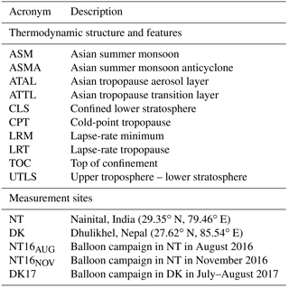
The measurements were conducted during three distinct periods of time, including two extensive monsoon-season campaigns, in NT in 2016 (2–31 August, 30 balloon soundings: NT16AUG) and in DK in 2017 (30 July–12 August, 28 balloon soundings: DK17), and one shorter post-monsoon campaign in NT (2–8 November 2016, 5 balloon soundings: NT16NOV) (note that a list of the main acronyms used in this paper, including the abbreviations of stations and campaign periods, is given in Table 1). The frequency of the soundings and the composition of the payloads varied depending on the meteorological conditions and the operational constraints. Various logistic limitations affected our DK17 campaign, resulting in a reduced measurement schedule (most notably, the number of backscatter measurements was limited). Nevertheless, important scientific data were collected. The DK17 campaign took place simultaneously with the StratoClim aircraft campaign, based at Kathmandu Airport (Nepal), which performed eight scientific flights using the high-altitude M55-Geophysica research aircraft.
All soundings employed meteorological latex balloons (TOTEX, Japan) that were filled with hydrogen gas in order to allow them to ascend at a rate of about 5 m s−1. The maximum burst altitude of these balloons is around 35 km, and more than 70 % of our soundings reached at least 30 km (see Table S1 in the Supplement). A standard meteorological radiosonde was used to host additional instruments through its XDATA interface (Oelsner and Tietz, 2017) and to transmit the data of all instruments to the ground station at a frequency of 1 Hz. In particular, we used RS41-SGP (Vaisala, Finland) radiosondes (Vaisala, 2017), and the DigiCORA MW41 sounding system (Vaisala, Finland) as a ground station (Vaisala, 2014). Additional instruments employed were an electrochemical concentration cell (ECC, manufacturer: EN-SCI, USA) (Komhyr, 1969) for the ozone (O3) mixing ratio, a cryogenic frost-point hygrometer (CFH, EN-SCI, USA) (Vömel et al., 2007, 2016) for the water vapor (H2O) mixing ratio, and the Compact Optical Backscatter Aerosol Detector (COBALD, MyLab, Switzerland) for aerosol backscatter.
For the pressure (p) and temperature (T) measurements analyzed in this work, the uncertainties of the RS41-SGP radiosondes(hereafter: RS41) given by the manufacturer are 0.6/1 hPa (at pressures lower/higher than 100 hPa) and 0.3/0.4 K (at altitudes lower/higher than 16 km), respectively. The performance of ECC sondes has been assessed by many studies (e.g., Smit et al., 2007), and the uncertainties are estimated to be 5–10 % in terms of O3 partial pressure. CFH is a frost-point hygrometer based on the chilled-mirror principle with an uncertainty of less than 10 % for the H2O mixing ratio up to an altitude of 28 km (Vömel et al., 2007). ECC and CFH have been regularly deployed in the ASM region since 2009 (Bian et al., 2012). COBALD is a detector for aerosol backscatter measurements at optical wavelengths of 455 nm (blue visible) and 940 nm (infrared) developed at ETH Zürich, and downscales the original backscatter sonde by Rosen and Kjome (1991) in weight and size. The COBALD is able to detect cirrus clouds (e.g., Brabec et al., 2012) as well as aerosol layers, such as the ATAL (Vernier et al., 2015). In addition, one RS92-SGP radiosonde (Vaisala, Finland) was added to almost all of the payloads for an intercomparison with the performance of the RS41 radiosondes (not discussed in this paper). Finally, we note that due to logistical constraints, the first two soundings in NT16AUG employed iMet-1-RSB radiosondes (InterMet, USA) (InterMet, 2006), which offer the XDATA interface (Wendell and Jordan, 2016) and utilize SkySonde version 1.9 (Jordan and Hall, 2016) as data acquisition software, instead of RS41.
Table 2Number of balloon soundings performed for each instrument and campaign period. The number of soundings with instrumental malfunctions is displayed in parentheses (CFH refers to the number of failures and contamination events, respectively). Early burst is defined as a burst altitude < 25 km.

* Note that iMet radiosondes were used for the first two soundings in NT16AUG, instead of RS41 (see Sect. 2).
Table 3Mean values of altitude (z), pressure (p), potential temperature (θ) and temperature (T) of the lapse-rate minimum (LRM), lapse-rate tropopause (LRT), cold-point tropopause (CPT) and top of confinement (TOC) levels during the three campaign periods, NT16AUG, NT16NOV and DK17.
Note that for NT16NOV, the definition of TOC is not applicable (n/a).
In this study, we use the pressure measured by RS41 as the main vertical coordinate for all instruments. All variables are binned in pressure intervals of 1 hPa for p > 300 hPa, and 0.5 hPa for p < 300 hPa, yielding an improved signal-to-noise ratio and a dataset with consistent vertical levels. This binning corresponds to a vertical resolution of approximately 25 m in the UTLS. A quality check is performed for all instruments, based on an interpretation of their house-keeping data, and data points showing anomalous behavior are rejected. In this context, the contamination of CFH measurements deserves a special mention, as this effect was observed in a significant number of cases. It is seen in the drift towards high frost-point temperatures in the stratosphere, corresponding to water vapor mixing ratios exceeding physical constraints (see Fig. S1 in Supplement), which we attribute to the deposition of supercooled water droplets onto the inner walls of the instrument's inlet tube while passing through mixed-phase clouds. This hypothesis is currently the subject of a dedicated modeling study. To avoid instrumental artifacts such as these, we do not accept H2O mixing ratio measurements higher than 10 ppmv in the stratosphere for the analysis in this paper, which are unrealistic, as well as all measurements at pressures below 20 hPa (see Sect. 3). Ice saturation (Sice), i.e., relative humidity with respect to ice, is calculated using the frost-point temperature measured by CFH, the air temperature measured by RS41 and the parameterization for saturation vapor pressure over ice by Murphy and Koop (2005). The COBALD data are expressed as backscatter ratio (BSR), i.e., the ratio of the total-to-molecular backscatter coefficient. This is calculated by dividing the total measured signal by its molecular contribution, which is computed from the atmospheric extinction according to Bucholtz (1995), and using air density derived from the measurements of temperature and pressure (Cirisan et al., 2014). The COBALD BSR uncertainty as inferred by this technique is estimated to be around 5 % (Vernier et al., 2015).
The number of deployments of each instrument during the different campaign periods is summarized in Table 2. A full list of all 63 balloon soundings with date and time of launch, payload description, burst altitude and notes on malfunctions and contamination events is given in Table S1 in the Supplement. Note that, for the conversion of pressure to geometric altitude (z), mean profiles of p vs. z measured by RS41 are also shown in Fig. S2 in the Supplement.
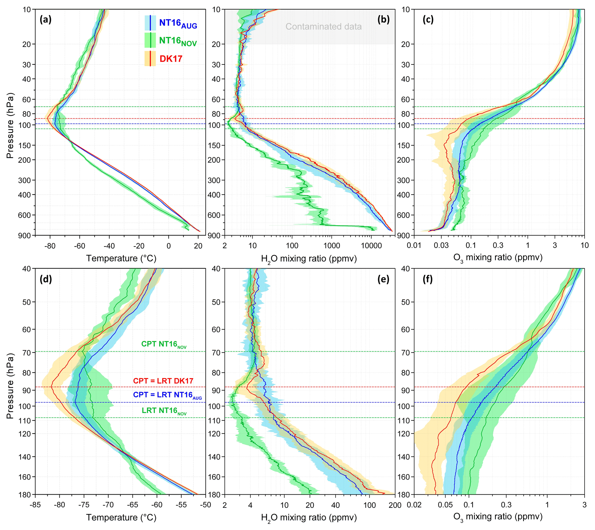
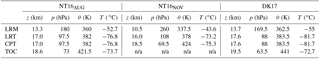
Figure 1Mean profiles (solid lines) and standard deviations (colored shading) of all measurements of temperature from RS41 (a, d), the H2O mixing ratio from CFH (b, e) and the O3 mixing ratio from ECC (c, f) as a function of pressure, for NT16AUG (blue), NT16NOV (green) and DK17 (red). Dashed lines indicate the pressure levels of the average cold-point tropopause (CPT) and lapse-rate tropopause (LRT) for the different datasets. Measured profiles from the surface to 10 hPa (a–c). A zoomed in profile of the tropopause region (40–180 hPa) (d–f). The grey shaded area in (b) indicates the region of contaminated CFH data (see Sect. 3).
Figure 1 shows mean profiles and standard deviations of temperature, the H2O mixing ratio and the O3 mixing ratio calculated from all measurements performed during the three campaign periods, namely NT16AUG (blue), NT16NOV (green) and DK17 (red). Figure 1a–c show the entire measured profiles, while Fig. 1d–f show a zoomed in profile of the UTLS region. In this section we briefly discuss their main features. Aerosol backscatter measurements will be discussed in Sect. 6.
In the troposphere, average H2O mixing ratios differ by up to a factor of 40 between the dry season(November) and the ASM season (July–August). Massive latent heat release by condensation during the wet period, in contrast to dry conditions in winter, is reflected in different lower tropospheric lapse rates for the two seasons, with about 5.5 K km−1 in July–August and 8 K km−1 in November. This is consistent with the meridional shift of the intertropical convergence zone (ITCZ) and the associated deep convection patterns in the Asian sector, which reach about 30∘ N in boreal summer (Lawrence and Lelieveld, 2010). Lower tropospheric O3 in NT16AUG compared to NT16NOV is likely due to the enhanced washout of ozone precursor gases during the monsoon season. Higher tropospheric O3 in NT16AUG vs. DK17 might be related to photochemical smog transport from the New Delhi urban area and the highly populated Indo-Gangetic Plain (e.g., Kumar et al., 2010).
The structure of the tropopause region is very different during the three measurement periods. In contrast to the sharp cold-point tropopause (CPT) of the ASM season, the November measurements show an almost isothermal layer above the lapse-rate tropopause (LRT, defined according to the World Meteorological Organization: WMO, 1957); therefore, in NT16AUG and DK17 the LRT coincides with the CPT, while in NT16NOV the average LRT and CPT are about 2.5 km apart. Seasonal variations of the LRT–CPT separation are consistent with Munchak and Pan (2014) and related to the varying meridional position of the jet stream (see Sect. 4.1). Interestingly, comparing the two ASM season datasets also reveals significant differences. The average CPT is 10 hPa higher (88 vs. 97.5 hPa), corresponding to about 600 m in altitude, and 5 K colder (−81.7 vs. −76.8 ∘C) in DK17 compared to NT16AUG. Water vapor in the UTLS is minimum in NT16NOV, with mixing ratios around 2.5 ppmv above the LRT. During the ASM, UTLS H2O is higher, but different vertical distributions are observed. In NT16AUG, H2O mixing ratio decreases monotonically with altitude, with a mean value of 6.8 ppmv at the CPT. In DK17, the H2O mixing ratio shows a minimum at the CPT (3.5 ppmv), and a local maximum above it (6 ppmv). Mean altitude, pressure, potential temperature and temperature of the LRT and CPT for the three campaign periods are summarized in Table 3.
Lower stratospheric temperatures (20–60 hPa) differ by about 2–4 K between November and July–August, which is consistent with the climatological annual cycle of stratospheric temperature (Randel et al., 2003). Stratospheric H2O mixing ratios are in the range of 4–6 ppmv up to 20 hPa, with a slight increase with altitude due to the oxidation of methane. Above approximately 20 hPa (27 km), all CFH measurements show an unrealistic increase in the H2O mixing ratio, which is a measurement artifact. At such high altitudes and low air densities, outgassing from the balloon skin and the payload train can play a significant role in contaminating the humidity measurements (Kräuchi et al., 2016). Water vapor data in this range are not considered in this analysis. Differences in stratospheric ozone between NT16AUG and DK17 are likely due to interannual variability.
For relating the measurements to the large-scale atmospheric flow, here we analyze meteorological data from the European Center for Medium-Range Weather Forecast (ECMWF) for the three campaign periods.
4.1 Seasonal variability
Figure 2 illustrates the seasonal variability of the meteorological systems above the southern slopes of the Himalayas during NT16AUG (top row), NT16NOV (center) and DK17 (bottom row). The left column (Fig. 2a, c, e) shows latitude–pressure cross sections of potential vorticity (PV), potential temperature and total wind speed for NT (longitude 80∘ E, Fig. 2a, c) and DK (85∘ E, Fig. 2e), from ECMWF analysis data averaged over the time of the respective measurement periods. The right column (Fig. 2d, b, f) shows the average geopotential height at 100 hPa for the three measurement periods from ECMWF analysis data, superimposed with 2-week backward air mass trajectories initialized at 100 hPa at the time of each sounding during the three campaign periods. Trajectories are calculated using the Lagrangian analysis tool (LAGRANTO) (Wernli and Davies, 1997) using ERA-Interim reanalysis wind fields that are color-coded by pressure.
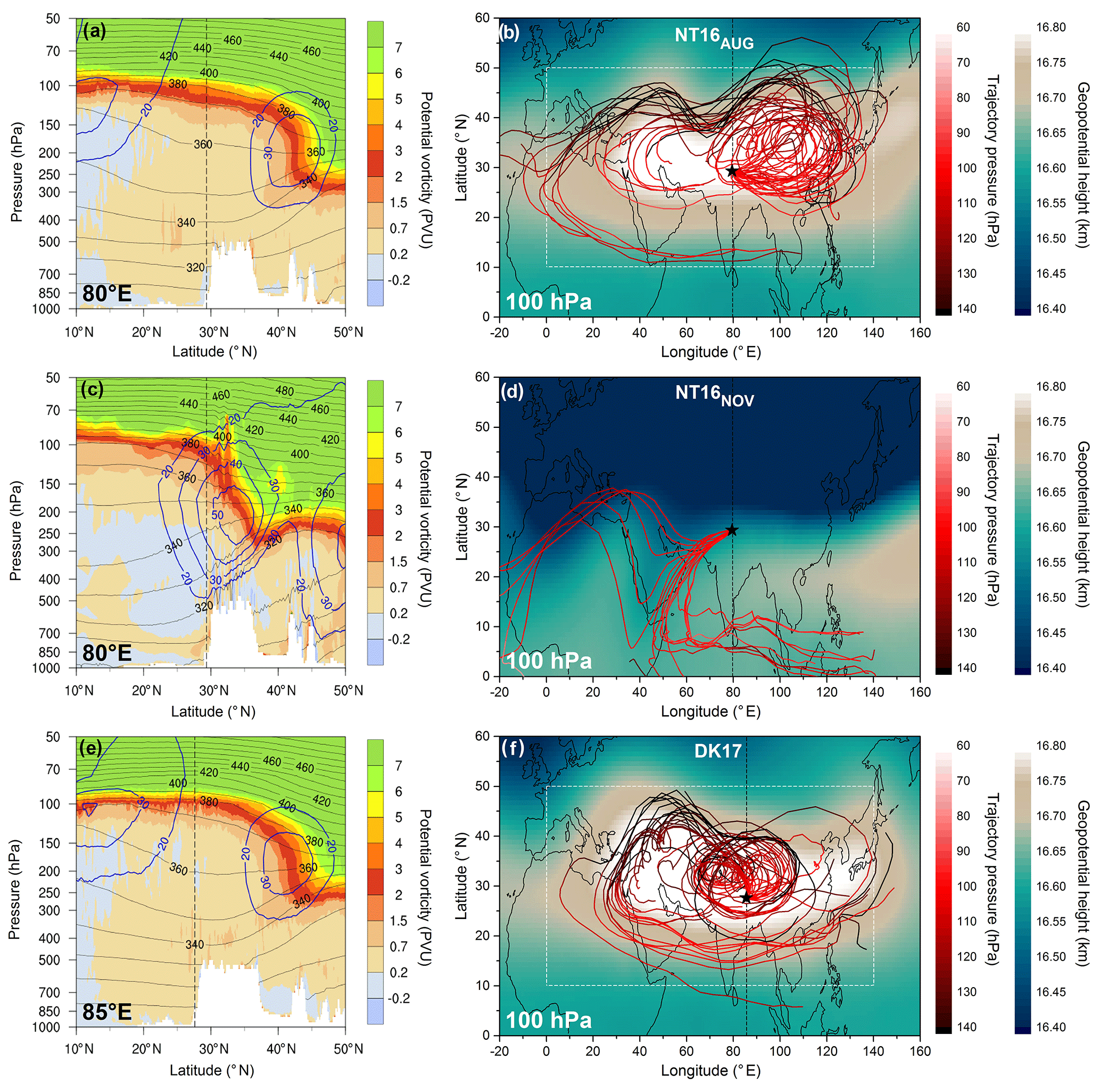
Figure 2(a, c, e) Latitude–pressure cross sections of potential vorticity (color scale), potential temperature (black contours, in K) and total wind speed (blue contours, in m s−1) from the ECMWF analysis data (horizontal resolution O1280 interpolated to a grid, vertical resolution L137, 6-hourly) averaged over the NT16AUG (a, longitude 80∘ E), NT16NOV (c, longitude 80∘ E) and DK17 (e, longitude 85∘ E) campaign time periods, as given in Table 2. Black dashed lines show the latitude of NT (a, c) and DK (e). (b, d, f) Geopotential height at 100 hPa from ECMWF analysis data averaged over the NT16AUG (b), NT16NOV (d) and DK17 (f) campaign time periods (color scale), and 2-week LAGRANTO backward trajectories calculated along ERA-Interim wind fields (horizontal resolution T255 interpolated to a 1∘ × 1∘ grid, vertical resolution L60), initialized at 100 hPa at the time of each balloon sounding in NT16AUG (b), NT16NOV (d) and DK17 (f), color-coded by pressure. Black dashed lines show the longitude of NT (a, c) and DK (e). The white dashed rectangle in (d, f) shows the approximated ASMA area used for the confined fraction calculation (10–50∘ N, 0–140∘ E; see Sect. 5.2). Note that, for NT16NOV, trajectories started 6 h before and 6 h after each sounding are also displayed (d).

Figure 3Time series of temperature (a, c, e, g) and the water vapor mixing ratio (b, d, f, h) as a function of pressure, from ECMWF operational analysis data (6-hourly, same horizontal and vertical resolution as given in the caption of Fig. 2) for NT (c, d, g, h) and DK (a, b, e, f) from 1 to 31 August 2016 (a–d) and from 20 July to 21 August 2017 (e–h).
During the NT16AUG and DK17 campaigns (Fig. 2a, b, e, f), our stations were located inside the ASMA vortex. The continental-scale anticyclonic motion is confined by the subtropical westerly jet stream to the north (40–45∘ N) and the equatorial easterly jet to the south (10–15∘ N). Both NT and DK were found in the average geopotential height region exceeding 16.8 km at 100 hPa during their respective measurement periods, which was the highest in the ASMA. Backward trajectories show that the UTLS flow on the southern slopes of the Himalayas is mainly easterly, following the southern branch of the ASMA, and transporting air masses which had already been confined inside the anticyclone for several days. During the 2 weeks prior to their respective measurement, the air masses sampled at 100 hPa during our campaigns had undergone net diabatic ascent at an average rate of 0.7 and 0.4 K day−1 (in isentropic coordinates) for NT16AUG and DK17, respectively. The equatorial easterly jet was slightly stronger and extended further north during the ASM season in 2017 (Fig. 2e) compared with 2016 (Fig. 2a); this is also reflected by the corresponding backward trajectories (Fig. 2b, f). North of the subtropical westerly jet, the dynamical tropopause (corresponding to PV = 3–4 PVU in this region and season: Kunz et al., 2011) decreases steeply with altitude.
After the end of the monsoon season, the subtropical westerly jet migrates southward to 30–35∘ N and intensifies in strength. Therefore, during the post-monsoon campaign NT16NOV (Fig. 2c, d), our station was located below the jet stream and the associated tropopause break, resulting in the large LRT–CPT separation discussed in Sect. 3. In contrast to the ASM season, in November the UTLS winds on the southern slopes of the Himalayas are mainly westerly and follow the subtropical jet stream. This is consistent with wind speed and wind direction measurements by RS41 shown in Fig. S3 in the Supplement. We also note that the large standard deviation of the UTLS temperature in NT16NOV (Fig. 1d) is likely related to the varying meridional position of the jet stream during the measurement period.
The dynamical features discussed above are consistent with the seasonal variations of the ITCZ, the jet streams and the ASM system in general, which are extensively discussed in previous literature, e.g., Lawrence and Lieleveld (2010), Munchak and Pan (2014), Ploeger et al. (2015), Garny and Randel (2016), Pan et al. (2016).
4.2 Interannual and regional variability
To assess whether the differences between the observations in NT16AUG and DK17 are mainly caused by geographic difference, and different associated mesoscale weather features, or by interannual variability between the ASM in the 2016 and 2017 seasons, Fig. 3 shows time series of the UTLS temperature (left column) and the H2O mixing ratio (right column) from ECMWF analysis data for both stations and both campaign periods.
In August 2016 (Fig. 3a–d) the UTLS was relatively warm at both locations, with CPT temperatures rarely dropping below −80 ∘C (DK was slightly colder than NT – 0.4 K on average at 100 hPa), and the H2O mixing ratio also never dropped below 4.5 ppmv at either site. The same day-to-day variability occurred at both locations with a time shift of about 6–12 h, which is consistent with DK being upstream of NT along the southern branch of the ASMA, and with wind speeds of around 20 m s−1 in the UTLS. In July–August 2017 (Fig. 3e–h), temperatures and H2O values and features were similar to 2016 until 3 August. Then, a period characterized by an extremely cold and dry tropopause began in both NT and DK, peaking between 7 and 10 August with a CPT colder than −83 ∘C and H2O mixing ratios lower than 3 ppmv. The minima were slightly more pronounced in DK than in NT but were correlated in time, suggesting that these features are related to a large-scale cooling and drying pattern occurring in the ASMA. We also note that a layer of high H2O rises to high altitudes (70–85 hPa) after 3 August (Fig. 3f), forming the local maximum above the CPT which was also found in our DK17 measurements (Fig. 1e). This feature is remarkable and not in accordance with more typical climatological conditions observed during NT16AUG.
Based on Fig. 3, we argue that the differences between the NT16AUG and DK17 datasets are not due to local meteorological effects, which appear to have a negligible impact on the UTLS temperature and H2O at the two measurement sites. Rather, these differences are attributed to interannual variability, and in particular to a period of an anomalously cold and dry UTLS on the southern slopes of the Himalayas, which occurred after 3 August 2017 and persisted on a large scale.
In this section we focus on analyzing the UTLS structure of the NT16AUG and DK17 measurements. The NT16NOV measurements will be discussed again in Sect. 6.
5.1 Asian tropopause transition layer (ATTL)
In the tropics, the thermodynamic transition between the troposphere and the stratosphere occurs over a layer of several kilometers in thickness, known as tropical tropopause layer (TTL). This layer is influenced by both upper tropospheric and lower stratospheric processes, and its properties control water vapor transport through the tropopause (e.g., Fueglistaler et al., 2009; Randel and Jensen, 2013). Amongst several different definitions of the TTL used in the literature, reviewed by Pan et al. (2014), Gettelman and de F. Forster (2002) identify its boundaries based on the temperature and potential temperature lapse rates only, which is particularly suited to balloon-borne measurements. In their definition, the upper boundary of the TTL is the CPT, and the lower boundary is the lapse-rate minimum (LRM), i.e., the point in altitude where the change of potential temperature (θ) with altitude (z) is minimum. This defines the TTL as the layer in which the temperature lapse rate switches from convectively dominated in the troposphere (small dθ∕dz, low stability), to radiatively controlled in the stratosphere (high dθ∕dz, high stability; Gettelman and de F. Forster, 2002). In addition, the LRM coincides with the mean convective outflow level (e.g., Gettelman and de F. Forster, 2002; Vömel et al., 2002; Paulik and Birner, 2012). Given the similarity between the UTLS region on the southern slopes of the Himalayas during the ASM season and that of the tropics, in this study we adopt the abovementioned definition of the TTL to study the thermal structure of our NT16AUG and DK17 datasets. However, as our measurement sites are not tropical in a geographical sense, we refer to the TTL in this region and season as the Asian tropopause transition layer (ATTL).
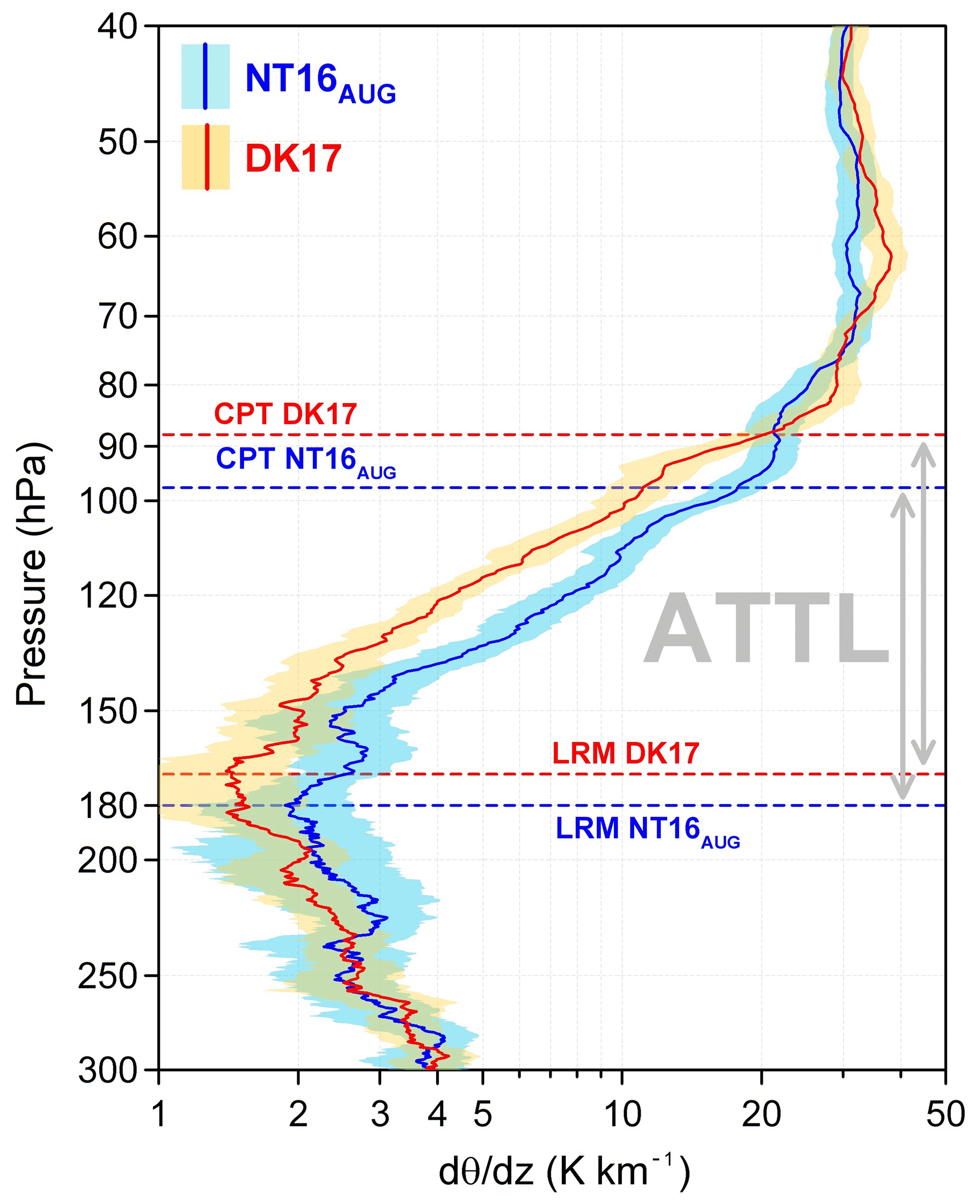
Figure 4Mean profiles (solid lines) and standard deviations (colored shading) of dθ∕dz as a function of pressure for NT16AUG (blue) and DK17 (red). Horizontal dashed lines show the mean LRM and CPT for NT16 (blue) and DK17 (red). The ATTL regions for the two datasets are highlighted by grey arrows. Note that the mean profiles and standard deviations of dθ∕dz were smoothed with a ±5 hPa (about 250 m) moving average to reduce the noise contributions from the geometric altitude measurement by RS41.
Figure 4 shows mean profiles and standard deviations of dθ∕dz as a function of pressure for the two ASM season datasets. The average LRM is found at lower pressure in DK17 compared to NT16AUG (169.5 vs. 180 hPa), corresponding to a roughly 400 m altitude difference, and the minimum in dθ∕dz of DK17 is more pronounced (1.5 vs. 2 K km−1). This suggests that convection reached higher altitudes, on average, in the ASM in 2017 compared to 2016 on the southern slopes of the Himalayas (at least during our measurement periods). The average ATTL boundaries in terms of pressure (potential temperature) are 180–97.5 hPa (360–382 K) for NT16AUG and 169.5–88 hPa (362.5–383.5 K) for DK17 (see Table 3; note that the data are binned with respect to pressure and the given potential temperature values are the average θ in the pressure levels where the LRM and CPT occur). We also observe that, due to the colder temperatures, the isentropic levels in DK17 are shifted to lower pressures compared to NT16AUG (see Fig. S4 in the Supplement), meaning that the large altitude difference between the two LRMs and CPTs in NT16AUG compared to DK17 (400–600 m) becomes small in isentropic coordinates (1.5–2 K).
5.2 Confined lower stratosphere (CLS)
Since the anticyclonic circulation extends up to above the CPT, it is important for interpreting the observed vertical gradients of chemical species and aerosols to quantify the vertical extent of the ASMA in the lower stratosphere. Here we estimate the top of the horizontal confinement effect of the ASMA during the NT16AUG and DK17 campaign periods by means of air mass trajectories. For this, we consider 2-week LAGRANTO backward trajectories initialized at 5 hPa intervals between 40 and 150 hPa at the time of each balloon sounding in NT16AUG and DK17 (i.e., same as in Fig. 2b, f, for 100 hPa), and 6 h before and 6 h after each sounding, using ERA-Interim wind fields. For each pressure level, we calculate the “confined fraction” of trajectories, defined as the fraction of trajectories which were already located inside the anticyclone 2 weeks before the measurements. For this purpose, based on the average geopotential height fields shown in Fig. 2, we approximate the ASMA area as the box of 10–50∘ N latitude, 0–140∘ E longitude (see the white dashed rectangle in Fig. 2b, f).
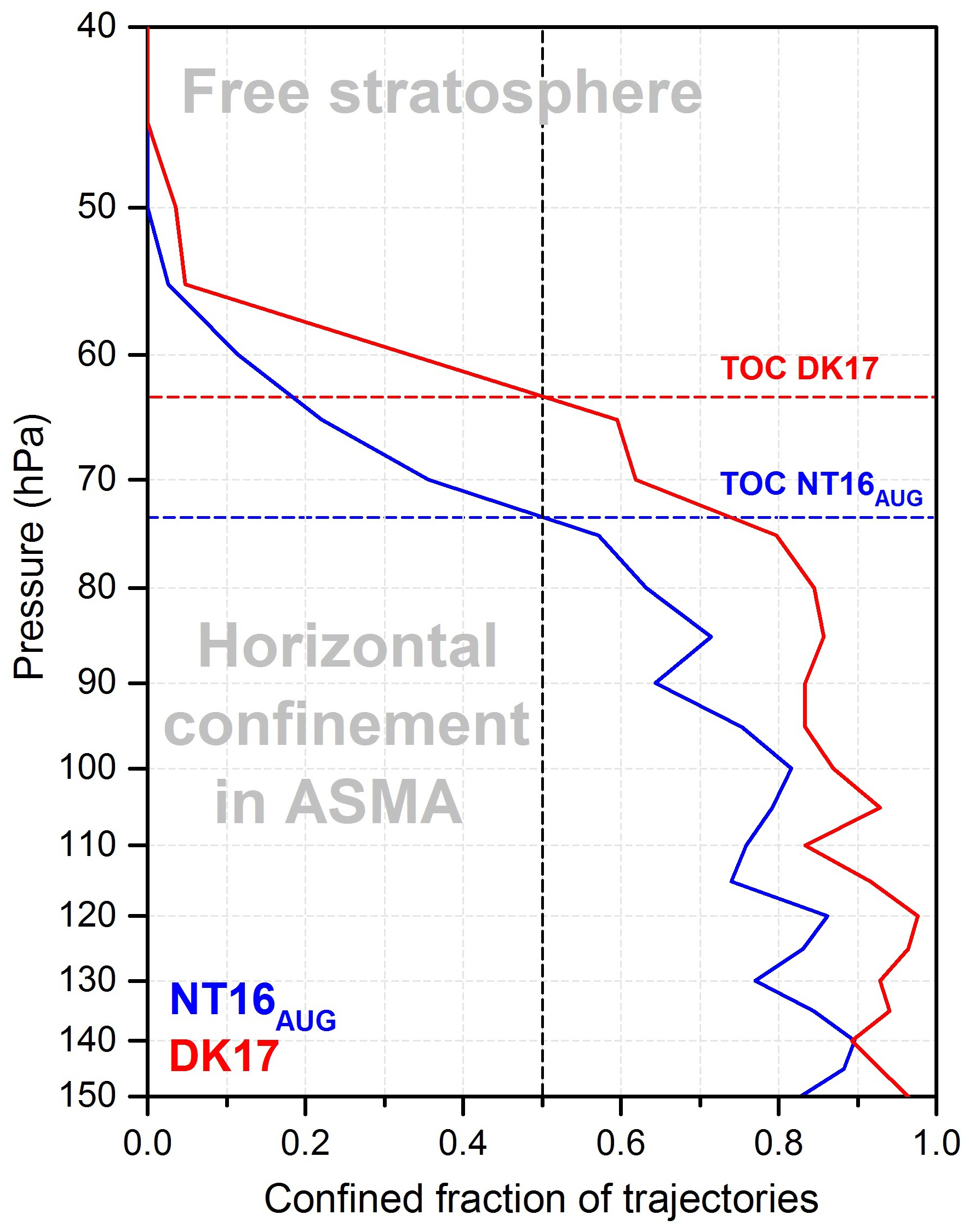
Figure 5Confined fraction of trajectories (see Sect. 5.2) as a function of pressure for the NT16AUG (blue) and DK17 (red) campaign periods. Dashed lines mark the TOC level for NT16 (blue) and DK17 (red) and the 50 % confined fraction threshold (black).
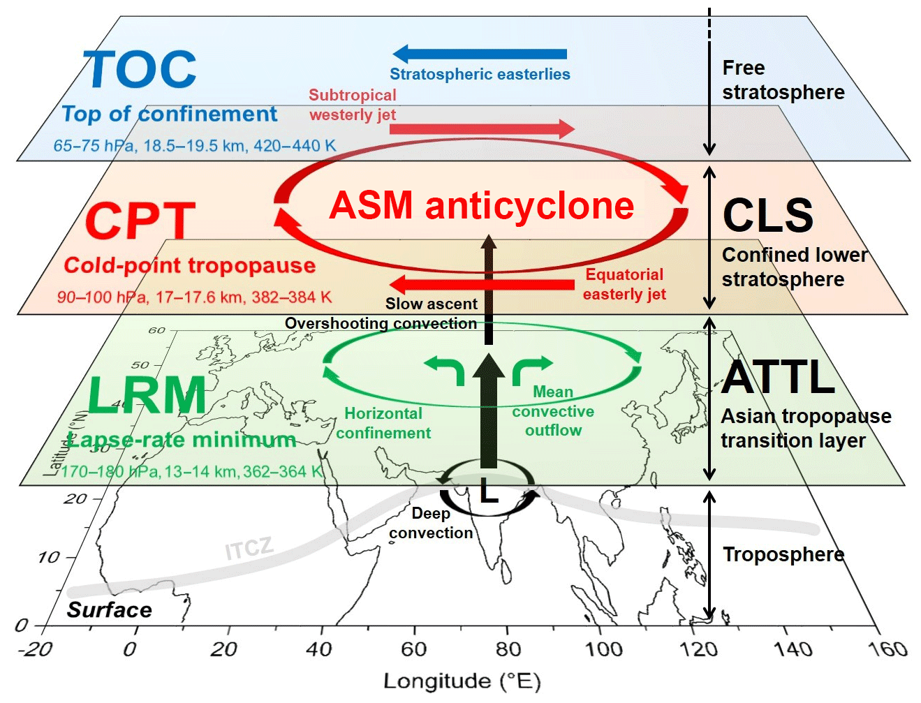
Figure 6Schematics of the vertical structure of the UTLS above the southern slopes of the Himalayas. The Asian summer monsoon anticyclone (ASMA) consists of two layers, the Asian tropopause transition layer (ATTL) and the confined lower stratosphere (CLS). These layers are confined by three levels: the lapse-rate minimum (LRM, green surface), the cold-point tropopause (CPT, red) and the top of confinement (TOC, blue). Dynamical features and relevant transport processes discussed in the paper are also sketched. Approximated pressure, altitude and potential temperature levels of the TOC, CPT and LRM derived from NT16AUG and DK17 measurements are displayed on the respective surfaces.
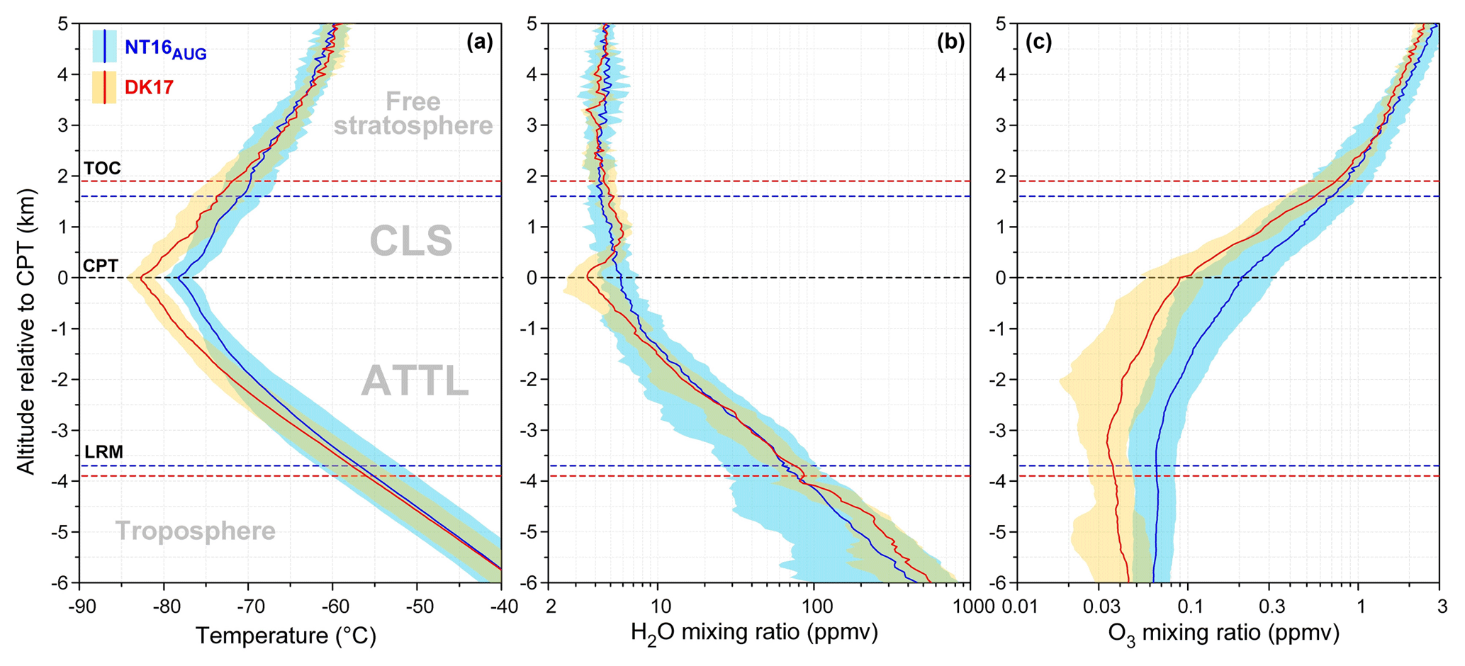
Figure 7Mean profiles (solid lines) and standard deviations (colored shading) of temperature (a), the H2O mixing ratio (b) and the O3 mixing ratio (c) as a function of altitude relative to the CPT, for NT16AUG (blue) and DK17 (red). Dashed lines show the CPT (black) and the average LRM and TOC levels for NT16 (blue) and DK17 (red) (see the labels in a). The four layers defined in Sect. 5.1 (troposphere, ATTL, CLS and free stratosphere) are identified using grey labels.
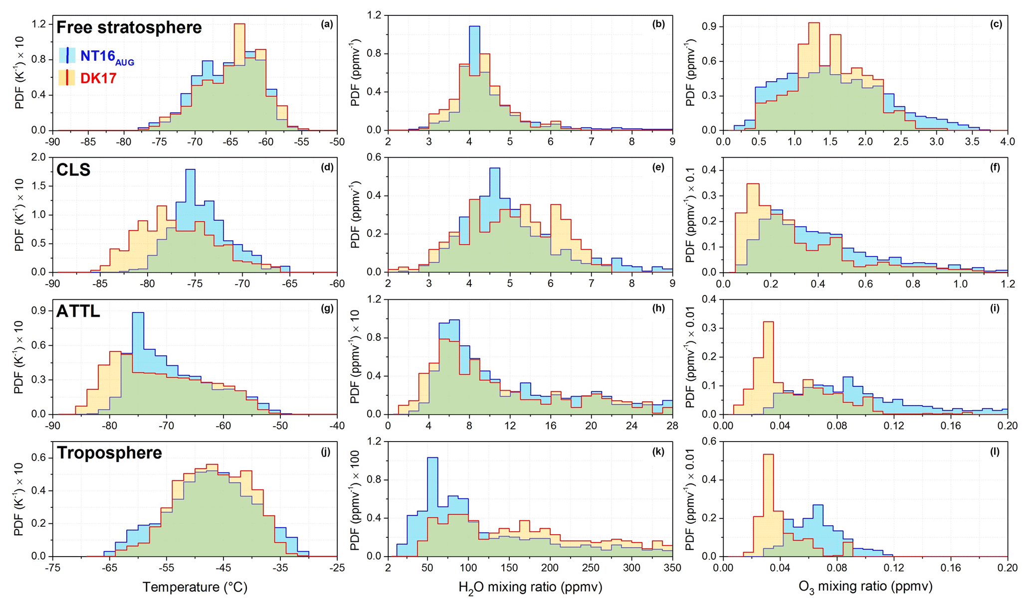
Figure 8Probability density functions (PDFs) of temperature (a, d, g, j), the H2O mixing ratio (b, e, h, k) and the O3 mixing ratio (c, f, i, l), calculated in the free stratosphere (a–c), CLS (d–f), ATTL (g, h) and troposphere (j–l) altitude regions as defined in Sect. 5.1, for NT16AUG (blue) and DK17 (red).
Figure 5 shows the resulting confined fractions for NT16AUG and DK17 as a function of pressure. In both campaign periods, the confined fraction is high (above 60 %) up to 70–80 hPa, while above this pressure level it sharply decreases to zero. Confinement is higher for DK17 than for NT16AUG throughout the entire UTLS, which is qualitatively consistent with the backward trajectories shown in Fig. 2. Based on these curves, we define the top of confinement (TOC) as the level of confined fraction equal to 50 %, corresponding to 73 hPa in NT16AUG and 63.5 hPa in DK17. This level separates altitudes that are affected by horizontal confinement in the ASMA (below TOC) from the confinement-free stratosphere above the ASMA (above TOC). Note that the mean altitude and potential temperature levels of the TOC derived from the balloon measurements are given in Table 3.
Following the definition of the TOC, we further define the confined lower stratosphere (CLS) as the region of altitudes above the CPT and below the TOC. The CLS is the layer of lower stratosphere which is subject to confinement in the ASMA, in contrast to the free stratosphere above the anticyclonic vortex (i.e., above TOC). Figure 6 illustrates the vertical structure of the UTLS above the southern slopes of the Himalayas during the ASM season according to the abovementioned definitions of the ATTL and the CLS. In the following, we refer to this framework of significant levels and layers to discuss the vertical distributions and variability of water vapor, ozone, ice saturation and aerosols in the ASMA.
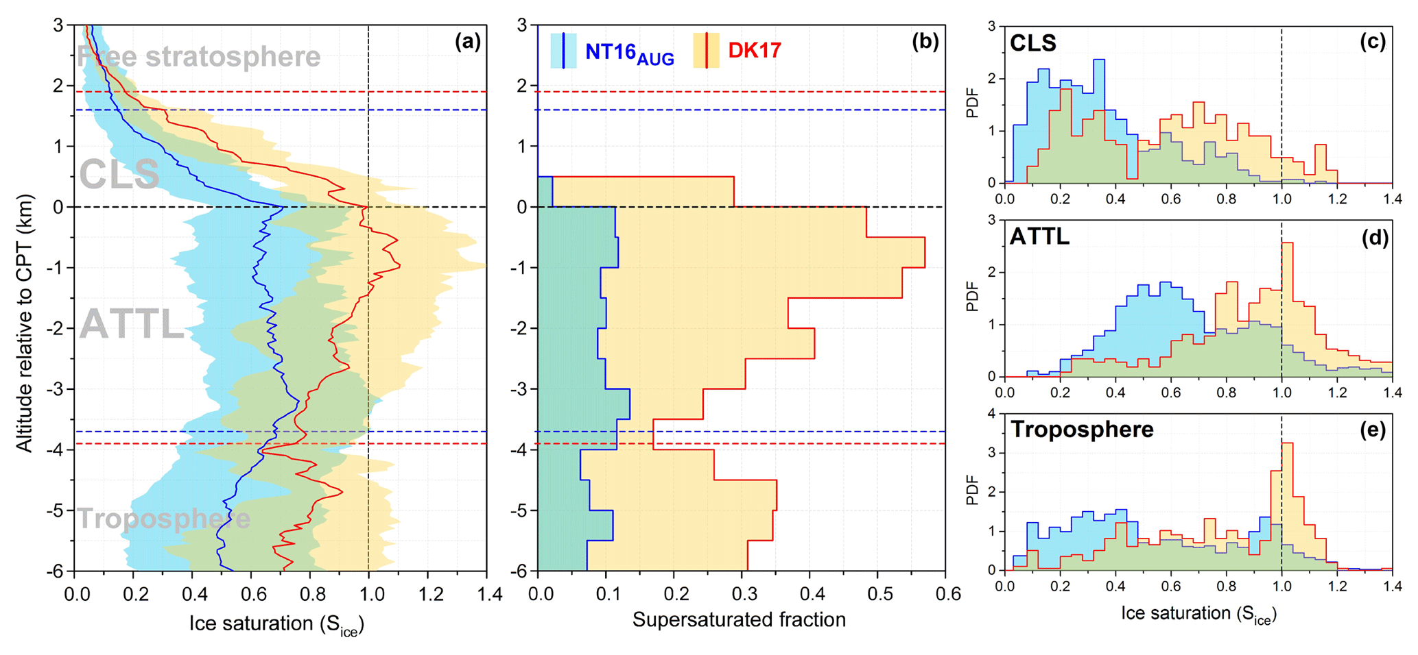
Figure 9(a) Mean profiles and standard deviation of ice saturation (Sice) as a function of altitude relative to the CPT, for NT16AUG (blue) and DK17 (red). (b) The supersaturated fraction (i.e., fraction of measurements with Sice > 1) as a function of altitude relative to the CPT. (c, d, e) PDFs of ice saturation in the CLS, ATTL and troposphere altitude regions, respectively.
5.3 Water vapor and ozone
To analyze our H2O and O3 measurements in relation to the thermodynamic structure of the UTLS, for each balloon sounding we define the altitude relative to the CPT as a new vertical coordinate. Figure 7 shows mean profiles and standard deviations of temperature, the H2O mixing ratio and the O3 mixing ratio in this coordinate system (note that, besides the CPT in black, the mean LRM and TOC levels are shown by blue dashed lines for NT16AUG and red dashed lines for DK17). Figure 8 shows the probability density functions (PDFs) of temperature (left column), the H2O mixing ratio (center) and the O3 mixing ratio (right column) calculated in the free stratosphere (Fig. 7a–c), CLS (Fig. 7d–f), ATTL (Fig. 7g–i) and troposphere (Fig. 7j–l) regions, for NT16AUG and DK17. The PDFs of the free stratosphere region are calculated for altitudes between the TOC and CPT + 5 km, while the troposphere PDFs are calculated for altitudes between the CPT and 6 km and LRM, i.e., covering the whole range of altitudes (with respect to CPT) as shown in Fig. 7.

Figure 10Examples of thin cirrus clouds measured during four individual soundings of the NT16AUG campaign (a–d) and two soundings of the DK17 campaign (e, f). Solid lines show temperature (black), ice saturation (light blue), BSR at 455 nm (BSR455, blue), BSR at 940 nm (BSR940, red) and the color index (green). Vertical dashed lines mark the Sice = 1 (light blue) and the color index = 7 (green) thresholds, used for cloud-filtering (see Sect. 6.1). Sounding identification numbers are noted in black in the top-right corner of each panel; for the date, time and payload of each sounding, see Table S1 in the Supplement.
The water vapor mixing ratio in DK17 shows a minimum at the CPT and a local maximum in the CLS (Fig. 7b), centered about 1 km above the local CPT (i.e., not the average CPT, but evaluated for each profile individually). The H2O minimum is conceivably due to the unusually high frequency of the occurrence of ice clouds near the CPT in DK17, which depletes water vapor from the gas phase in favor of the condensed phase and results in a strongly dehydrated CPT (see Sect. 5.4). The isolated H2O maximum in the CLS is consistent with hydration by overshooting convective updrafts; this process injects ice crystals above the CPT, which then evaporate and release localized “pockets” of moist air. Convective updrafts overshooting the CPT were observed by Corti et al. (2008), and a similar hydration mechanism was hypothesized by Dauhut et al. (2015, 2016).
In both NT16AUG and DK17, the PDFs of the H2O mixing ratio show higher water vapor in the CLS (Fig. 8e) compared to the free stratosphere (Fig. 8b). In particular, the PDFs in the CLS are broad (3–7 ppmv) and skewed towards high values, while the PDFs in the free stratosphere are narrow (3–5 ppmv) and show the expected distribution of background stratospheric water vapor. The high H2O mixing ratios in the CLS in DK17 are obviously related to the previously discussed isolated maximum, yet the enhanced frequency of occurrence of high H2O mixing ratios is also observed in NT16AUG, despite no local maximum being found in this dataset. This is consistent with the slow ascent of moist convective outflow air within the confined anticyclone, and may, in part, reflect the decreasing frequency of overshooting convective tops with altitude in NT16AUG.
The ozone mixing ratio in DK17 shows a minimum slightly above the LRM (Fig. 7c), which is characteristic of deep convection, rapidly transporting ozone-poor air from the boundary layer to the convective outflow level (e.g., Gettelman and de F. Forster, 2002; Vömel et al., 2002; Paulik and Birner, 2012). The absence of this feature in NT16AUG suggests that the average age of air, meant as the time elapsed since the last interaction with deep convection, was higher in NT16AUG compared with DK17, such that the O3 minimum is smeared out by mixing and additional photochemical production (which is enhanced in the ASMA due to the enrichment in ozone precursors; Gottschaldt et al., 2018). The higher dilution of the convective signature in NT16AUG vs. DK17 is also consistent with the absence of an H2O maximum above the CPT in NT16AUG (Fig. 7b), and with the higher frequency of the occurrence of low O3 mixing ratios in DK17 compared with NT16AUG in the ATTL and CLS (Fig. 8f, i).
In summary, both the NT16AUG and DK17 datasets show evidence of deep convection extending into the CLS, i.e., up to 1.5–2 km above the CPT. Convective features, such as low O3 in the ATTL and high H2O in the CLS, are more pronounced in DK17 than in NT16AUG, indicating that DK17 likely sampled fresh convective outflow more frequently than NT16AUG. This is also consistent with the higher altitude of the LRM in DK17 compared to NT16AUG (Fig. 4) and suggests that convective activity on the southern slopes of the Himalayas was more frequent during the ASM season in 2017 than in 2016.
Transport to the CLS is likely due to a combination of different processes, including overshooting convection, slow diabatic ascent and adiabatic transport from regions with a higher CPT potential temperature in the ASMA (discussed in Sect. 7). Although we do not quantitatively evaluate these processes, we argue that the horizontal confinement effect of the ASMA plays an important role in shaping the vertical distributions of H2O and O3 above the CPT, by keeping the moist convective outflow horizontally confined (while it continues to rise slowly) and thereby increasing the frequency of occurrence of air parcels with high H2O and low O3 above the CPT. This is supported by the fact that differences in H2O and O3 between NT16AUG and DK17 vanish in the free stratosphere (Fig. 8a–c), which is in agreement with our trajectory-based definition of TOC. Further analysis will be required to disentangle the relevance of the different abovementioned transport processes in moistening the CLS.
5.4 Ice saturation
Figure 9 shows the mean profiles and standard deviations of ice saturation (Fig. 9a) and histograms of supersaturated fraction (Fig. 9b) as a function of altitude relative to the CPT, and PDFs of ice saturation calculated for the troposphere, ATTL and CLS regions (Fig. 9c–e). As a result of colder temperatures (see Fig. 7a), much higher and more persistent ice saturations were measured in DK17 than in NT16AUG throughout the entire ATTL. In both datasets, the average ice saturation is higher in the ATTL than in the troposphere, and in DK17 it shows a pronounced maximum with respect to average supersaturated conditions (i.e., more than 50 % of the measurements reach Sice > 1) in the 1.5 km directly below the CPT. In contrast, the supersaturated fraction is 10–15 % in NT16AUG over the same range of altitudes. The ATTL ice saturations and supersaturated fractions of NT16AUG are comparable with previous measurements from Lhasa and Kunming, China from 2009 to 2010 (Bian et al., 2012), while the measurements in DK17 range significantly higher. This suggests that the frequency of occurrence of cirrus clouds in the ASM season in 2017 was unusually high, which is likely the reason for the H2O minimum at the CPT observed in DK17 (Fig. 7b). Interestingly, we also note that ice supersaturations in DK17 frequently extend into the CLS, with about a 30 % supersaturated fraction in the first 500 m above the CPT (Fig. 9b, c). This implies that, in overshooting convective updrafts, ice crystals can regularly penetrate the CPT as condensed phase (e.g., see Fig. 10f) and hence efficiently hydrate the CLS.
In this section we analyze the aerosol and cloud backscatter measurements by COBALD, which have not been discussed so far. COBALD was originally designed to investigate ice cloud properties, including cirrus (e.g., Brabec et al., 2012; Cirisian et al., 2014) and polar stratospheric clouds (e.g., Engel et al., 2014), yet recent measurements from Lhasa, China, were also used for in situ detection of ATAL aerosols (Vernier et al., 2015, 2018). Here we address both aspects.
Since the BSR of aerosol droplets is 1–2 orders of magnitude smaller than that of cirrus clouds, the characterization of the ATAL requires cloud-filtering techniques to eliminate in-cloud measurements, and a large dataset for a statistically significant evaluation (e.g., 18 soundings are used in Vernier et al., 2015). We performed 17 COBALD soundings in NT16AUG, but due to logistical constraints only 3 could be realized during the DK17 campaign; furthermore, these soundings mostly sampled cloudy conditions near the CPT. For this reason, a clear-sky aerosol BSR profile could not be established from the DK17 dataset. Conversely, the three COBALD soundings available from NT16NOV are almost fully clear-sky measurements and therefore allow for the calculation of a clear-sky aerosol BSR profile. The NT16NOV measurements provide a useful reference state of background aerosols, without ASMA confinement and without a supply of aerosols and precursor gases from the monsoonal deep convection, for comparison with NT16AUG. In the following, we first provide an overview of the main characteristics of the observed cirrus clouds, and then detail the cloud-filtering technique and the ATAL detection during the year 2016.
6.1 Cirrus clouds
Figure 10 shows individual soundings as examples of thin cirrus clouds observed during the NT16AUG (Fig. 10a–d) and DK17 (e, f) campaigns. Along with the temperature and ice saturation profiles, we show BSR at 455 nm (BSR455), BSR at 940 nm (BSR940), and the color index (CI). The color index is defined as the 940-to-455 nm ratio of the aerosol component of BSR, i.e., CI = (BSR940−1) ∕ (BSR455−1). CI is independent of the number density; therefore, it is a useful indicator of particle size (e.g., Cirisian et al., 2014) as long as particles are sufficiently small, so that Mie scattering oscillations can be avoided. Based on the size-dependence of the CI, considerations regarding the typical size range of ice crystals and aerosol droplets, and the evaluation of ice saturation measurements by CFH, a threshold of CI = 7 was empirically developed to discriminate in-cloud (CI > 7) from clear-sky measurements (CI < 7) (Vernier et al., 2015). This helps discern the BSR features in Fig. 10 as either ice cloud or aerosol signal, and is also used as a threshold for cloud-filtering. For example, in sounding NT004 (Fig. 10a), the sharp feature at 145 hPa with a CI ≈ 10 is likely an ice cloud (note the concomitant ice supersaturation above the thin cloud layer, suggesting sedimentation), while the broad enhancement in BSR between 95 and 140 hPa without CI enhancement is the signal of the ATAL. The main common characteristics of the cirrus clouds in Fig. 10 is their very small spatial and optical thickness, with BSR940 < 20, while much larger values (BSR940 ≫ 100) are expected in homogeneously nucleated cirrus clouds, as often observed in the midlatitudes (e.g., Brabec et al., 2012; Cirisian et al., 2014), and as also shown by the thick outflow cirrus below 120 hPa in DK002 (Fig. 10f). Low BSR indicates low ice crystal number densities, suggesting that these clouds are most likely formed by heterogeneous nucleation on solid ice nuclei, rather than by homogeneous freezing of sulfate aerosol liquid droplets. This hypothesis is currently being investigated by a dedicated microphysical modeling study. Similarly thin cirrus clouds were observed in more than half of the COBALD soundings in NT16AUG (9 out of 17); therefore, they occur very frequently in the ASMA, and they were often found embedded within the ATAL (Fig. 10a, e).

Figure 11All clear-sky (i.e., aerosol only) data points (dots) and mean profiles (solid lines) of BSR455 as a function of pressure, for NT16AUG (blue) and NT16NOV (green). Black lines show the mean LRM (dashed), CPT (solid) and TOC (dashed) levels for NT16AUG. The troposphere, ATTL, CLS and free stratosphere regions are identified using grey labels, and the ATAL region is identified using a black arrow.
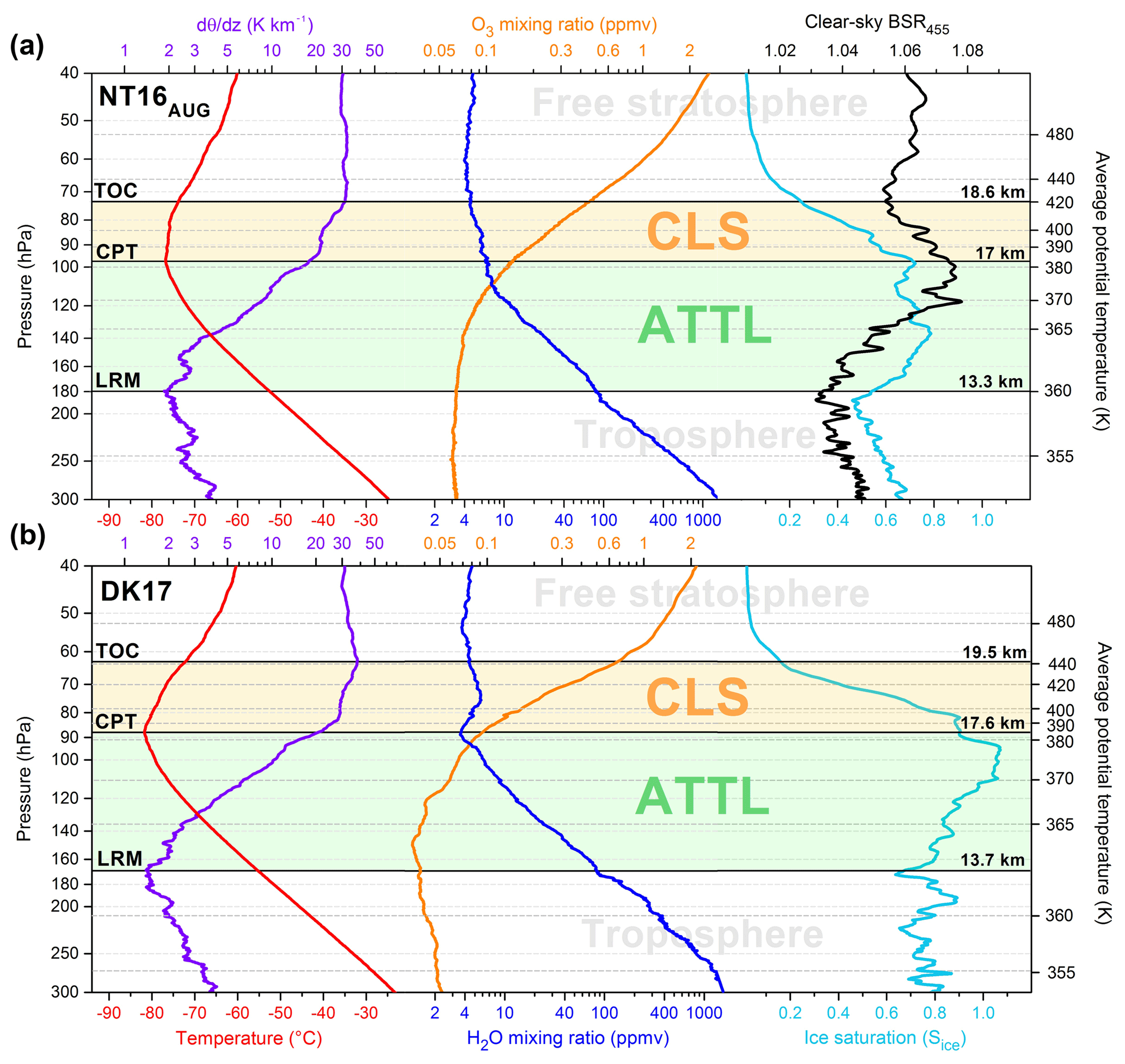
Figure 12Mean profiles of temperature (red), dθ∕dz (purple), the H2O mixing ratio (blue), the O3 mixing ratio (orange), ice saturation (light blue) and clear-sky aerosol BSR455 (black) as a function of pressure (left axis, light grey dashed lines) for NT16AUG (a) and DK17 (b). Average potential temperature levels are shown on the right axis and marked by dark grey dashed lines. Note that the pressure scale is the same for the two panels, and the potential temperature levels vary according to the measurements. The average CPT, LRM and TOC levels in the two datasets are marked by black solid lines. The ATTL and CLS layers are highlighted using light green and orange shading, respectively. Note that the mean profiles of dθ∕dz, ice saturation and clear-sky aerosol BSR455 are smoothed with a ±5 hPa (about 250 m) moving average (same as in Fig. 4).
6.2 ATAL during the ASM season 2016
Figure 11 shows all clear-sky (i.e., aerosol only) BSR455 data points and mean profiles from the NT16AUG and NT16NOV datasets. Similarly to Vernier et al. (2015), the cloud-filtering criterion that we applied consists of three thresholds from two independent measurements: BSR940 < 2.5 and CI < 7 from COBALD, and Sice < 0.7 from CFH. Only data points which simultaneously fulfill all of the three abovementioned specifications were classified as clear-sky and are shown in Fig. 11. The cloud-filtering method is illustrated using a scatter plot of BSR940 vs. CI, which is given in Fig. S5 in the Supplement.
In NT16AUG, a clear-sky BSR455 enhancement (i.e., a mean value exceeding 1.04) starting approximately at the LRM (180 hPa) and extending up to the TOC (73 hPa) is the signature of the ATAL (Fig. 11), showing intensity and vertical extent comparable to those derived by satellite retrievals and previous COBALD measurements (Vernier et al., 2015, 2018). The enhanced aerosol BSR455 covers both the ATTL and the CLS, with a maximum BSR455 at the CPT. The fact that the onset of the ATAL coincides with the LRM suggests that the mean convective outflow level is also the onset of horizontal confinement in the ASMA. The maximum BSR455 at the CPT is possibly an effect of colder temperatures, driving the partitioning of more condensable material (e.g., nitrates, see Vernier et al., 2018) to the aerosol phase in the ATAL. Above the CPT, the BSR455 enhancement gradually fades with altitude until the TOC as the horizontal confinement effect of the ASMA vanishes, which is consistent with the decreasing confined fraction of the backward trajectories shown in Fig. 5. Above the TOC, the ATAL signal merges with the Junge layer of stratospheric aerosols, which extends into the free stratosphere up to about 10 hPa. The clear-sky BSR455 enhancement is absent in NT16NOV at all altitudes in the UTLS (except for the Junge layer in the free stratosphere), showing that the ATAL does not outlive the breakup of the anticyclonic vortex and the lack of a supply of precursor gases by deep convection after the end of the ASM season.
We analyzed 63 balloon measurements of temperature, water vapor, ozone and aerosol backscatter, collected during 2016 and 2017 on the southern slopes of the Himalayas. The UTLS structure in this region exhibits a strong seasonal variability, with tropical features (sharp CPT) during the ASM, and midlatitudinal features (large LRT–CPT separation) during the post-monsoon season. To analyze the structure of the UTLS during the ASM season, we formulated a framework composed of three significant levels (LRM, CPT, TOC) and two layers (ATTL, CLS), identified from the temperature and potential temperature lapse rates and Lagrangian backward trajectories – this framework is illustrated by the schematics in Fig. 6. Figure 12 summarizes the mean profiles of temperature, dθ∕dz, the H2O mixing ratio, the O3 mixing ratio, ice saturation and aerosol BSR455 measured during NT16AUG (top panel) and DK17 (bottom panel), highlighting the relevance of these levels and layers.
During both of the ASM season campaigns, the isentropic level of the LRM (θ = 362–364 K) was higher than in previous measurements in the deep tropics (θ ≈ 345 K) (Gettelman and de F. Forster, 2002; Pan et al., 2014) and on the Tibetan Plateau (355–360 K) (Bian et al., 2012), suggesting that convection is deeply penetrating on the southern slopes of the Himalayas. The CPT (θ = 382–384 K) was also higher than at tropical sites (375 K) (Gettelman and de F. Forster, 2002; Pan et al., 2014), but lower than on the Tibetan Plateau (390 K) (Bian et al., 2012), which is consistent with the “bulging” of the CPT in the ASMA (e.g., Pan et al., 2016) and suggests an orographic influence. The average LRM and CPT occur at a higher altitude in DK17 than in NT16AUG (400–600 m), but due to the colder temperatures in DK17 (on average 5 K at the CPT), the shift in potential temperature space is small (1.5–2 K). We also note that the TOC coincides with a local maximum in the thermal stability profile (dθ∕dz) in DK17, which is the same feature as the level of maximum stability defined by Sunilkumar et al. (2017).
In both NT16AUG and DK17, high H2O and low O3 were found in the ATTL and CLS, which is the signature of deep convection, extending up to 1.5–2 km above the CPT. Convective features are more pronounced in DK17 than in NT16AUG, suggesting that convective activity on the southern slopes of the Himalayas was more intense during the ASM season in 2017 compared with 2016. In particular, an isolated H2O maximum in the CLS was observed in DK17, which we argue may be due to overshooting convection, as previously observed by Corti et al. (2008) and modeled by Dauhut et al. (2015, 2016).
The fact that the average CPTs in our datasets occur at lower potential temperatures than previously found above the Tibetan Plateau suggests that, in addition to slow ascent and overshooting convection (discussed in Sect. 5.3), isentropic transport from the Tibetan Plateau (below CPT) to the southern slopes of the Himalayas (above CPT) might also contribute to the high H2O observed in the CLS. Nevertheless, since the isentropic level of the CPT is subject to strong instantaneous perturbations associated with convection and wave activity (e.g., Boehm and Verlinde, 2000; Sherwood et al., 2003; Munchak and Pan, 2014; Muhsin et al., 2018), a conclusion based on just the average CPT from a limited number of profiles is to be taken with caution. Therefore, further investigations will be required to assess the relevance of the different transport pathways.
The high H2O observed in the CLS is particularly interesting due to its potential implications for stratospheric moistening. The air masses in the CLS have already crossed the CPT, and will unlikely be subject to further dehydration, so it appears that the high H2O in this layer is prone to being lifted further and mixed into the (drier) free stratosphere. However, it has been shown that vertical transport above the ASMA might not be very efficient due to the slow ascending velocities of the Brewer–Dobson circulation in this region and season, and that the most efficient transport pathway is quasi-horizontal transport through the horizontal boundaries of the ASMA and subsequent upwelling in the stratosphere above the deep tropics (Pan et al., 2016). Therefore, the fate of the air masses in the CLS (hence the moistening potential of the high H2O in this layer) needs to be addressed by explicitly taking the horizontal motion of the air into account, which we do not investigate in this work.
Cloud-filtering of the NT16AUG aerosol backscatter measurements reveals the signature of the ATAL, extending from the LRM to the TOC with maximum backscatter at the CPT, and with similar BSR enhancement as in previous measurements from Lhasa, China (Vernier et al., 2015). No aerosol enhancement was found in NT16NOV. In both NT16AUG and DK17, ice saturation is minimum at the LRM and increases in the ATTL, similarly to the tropics (Vömel et al., 2002). Due to the much colder temperatures, average Sice in DK17 is remarkably higher than in NT16AUG, in addition to being higher than previous measurements from the Tibetan Plateau (Bian et al., 2012). Numerous thin cirrus clouds were detected during the NT16AUG and DK17 campaigns (often embedded in the ATAL), and their optical properties suggest they might have been formed by heterogeneous freezing.
Our analysis provides a comprehensive and high-resolution overview of the UTLS structure and composition on the southern slopes of the Himalayas. The observed vertical distributions of water vapor, ozone and aerosols in the ASMA are in good agreement with the thermodynamically significant levels that we define (LRM and CPT), and the extents of enhanced H2O and aerosols (ATAL) above the CPT are in good agreement with the top of anticyclonic confinement estimated from air mass backward trajectories (TOC). Our approach based on significant levels, rather than fixed pressure or altitude stacks, also provides physically meaningful diagnostics for the comparison of our in situ measurements with global climate model outputs.
As often mentioned throughout this paper, a wide range of modeling, interpretation and comparison studies are ongoing, and aim to explore all of the different insights offered by this dataset, in addition to assessing its relevance in the context of stratospheric moistening via the ASMA system and related transport pathways. These investigations include microphysical modeling, Lagrangian trajectory analyses, instrumental studies and comparisons with other in situ measurements, such as the airborne measurements of M55-Geophysica during the StratoClim 2017 aircraft campaign and balloon soundings performed from various stations on the Tibetan Plateau from 2013 to 2017, as well as comparisons with different global modeling products.
Data are available from the authors upon request.
The supplement related to this article is available online at: https://doi.org/10.5194/acp-18-15937-2018-supplement.
SB wrote the paper and produced all figures (except Fig. 2a, c, e). SB, TJ, PO, SH, BBS, KRK, SS, SM and DS made the measurements. SB, TJ, FGW, BPL, YP, HJ, RD, MN, MR, SF and TP provided technical, scientific and logistic support for the measurements. BBS, MN, SS and SF provided logistic support for the measurements in Nainital (India). RK, JK and MR provided logistic support for the measurements in Dhulikhel (Nepal). MB supported the analysis of the ECMWF data and produced Fig. 2a, c, e. SB and TP coordinated all measurements. All authors proofread the text.
The authors declare that they have no conflict of interest.
The research leading to these results received funding from the European
Community's Seventh Framework Programme (FP7/2007–2013) under grant
agreement no. 603557 and the Swiss National Science Foundation under project
no. 200021-147127. The use of the ECMWF operational and ERA-Interim data is
gratefully acknowledged. Support from the Director ARIES and the ISRO ATCTM
project is highly acknowledged regarding the observations at Nainital. Support from
the HiCCDRC group from Kathmandu University is highly acknowledged regarding the
observations at Dhulikhel. Maxi Boettcher acknowledges funding from the Swiss
National Science Foundation via grant no. 200020-165941. The author Simone
Brunamonti thanks Federico Fierli and Laura Pan for inspiring
discussions. Edited by: Farahnaz Khosrawi
Reviewed by: two anonymous referees
Bergman, J. W., Fierli, F., Jensen, E. J., Honomichl, S., and Pan, L. L.: Boundary layer sources for the Asian anticyclone: Regional contributions to a vertical conduit, J. Geophys. Res.-Atmos., 118, 2560–2575, https://doi.org/10.1002/jgrd.50142, 2013.
Bian, J., Pan, L. L., Paulik, L., Vömel, H., Chen, H., and Lu, D.: In situ water vapor measurements in Lhasa and Kunming during the Asian summer monsoon, Geophys. Res. Lett., 39, L19808, https://doi.org/10.1029/2012GL052996, 2012.
Boehm, M. T. and Verlinde, J.: Stratospheric influence on upper tropospheric tropical cirrus, Geophys. Res. Lett., 27, 3209–3212, 2000.
Brabec, M., Wienhold, F. G., Luo, B. P., Vömel, H., Immler, F., Steiner, P., Hausammann, E., Weers, U., and Peter, T.: Particle backscatter and relative humidity measured across cirrus clouds and comparison with microphysical cirrus modelling, Atmos. Chem. Phys., 12, 9135–9148, https://doi.org/10.5194/acp-12-9135-2012, 2012.
Bucholtz, A.: Rayleigh-scattering calculations for the terrestrial atmosphere, Appl. Optics, 34, 15, 1995.
Cirisan, A., Luo, B. P., Engel, I., Wienhold, F. G., Sprenger, M., Krieger, U. K., Weers, U., Romanens, G., Levrat, G., Jeannet, P., Ruffieux, D., Philipona, R., Calpini, B., Spichtinger, P., and Peter, T.: Balloon-borne match measurements of midlatitude cirrus clouds, Atmos. Chem. Phys., 14, 7341–7365, https://doi.org/10.5194/acp-14-7341-2014, 2014.
Corti, T., Luo, B. P., de Reus, M., Brunner, D., Cairo, F., Mahoney, M. J., Martucci, G., Matthey, R., Mitev, V., dos Santos, F. H., Schiller, C., Shur, G., Sitnikov, N. M., Spelten, N., Vössing, H. J., Borrmann, S., and Peter, T.: Unprecedented evidence for deep convection hydrating the tropical stratoshpere, Geophys. Res. Lett., 35, L10810, https://doi.org/10.1029/2008GL033641, 2008.
Dauhut, T., Chaboureau, J.-P., Escobar, J., and Mascart, P.: Large-eddy simulations of Hector the convector making the stratosphere wetter, Atmos. Sci. Lett., 16, 135–140, https://doi.org/10.1002/asl2.534, 2015.
Dauhut, T., Chaboureau, J.-P., Escobar, J., and Mascart, P.: Giga-LES of Hector the Convector and Its Two Tallest Updrafts up to the Stratosphere, J. Atmos. Sci., 73, 5041–5060, https://doi.org/10.1175/JAS-D-16-0083.1, 2016.
Dethof, A., O'Neill, A., Slingo, J. M., and Smit, H. G. J.: A mechanism for moistening the lower stratosphere involving the Asian summer monsoon, Q. J. Roy. Meteorol. Soc., 125, 1079–1106, 1999.
Engel, I., Luo, B. P., Khaykin, S. M., Wienhold, F. G., Vömel, H., Kivi, R., Hoyle, C. R., Gross, J.-U., Pitts, M. C., and Peter, T.: Arctic stratospheric dehydration – Part 2: Microphysical modeling, Atmos. Chem. Phys., 14, 3231–3246, https://doi.org/10.5194/acp-14-3231-2014, 2014.
Fadnavis, S., Semeniuk, K., Pozzoli, L., Schultz, M. G., Ghude, S. D., Das, S., and Kakaktar, R.: Transport of aerosols into the UTLS and their impact on the Asian monsoon region as seen in a global model simulation, Atmos. Chem. Phys., 13, 8771–8786, https://doi.org/10.5194/acp-13-8771-2013, 2013.
Fadnavis, S., Schultz, M. G., Semeniuk, K., Mahajan, A. S., Pozzoli, L., Sonbawne, S., Ghude, S. D., Kiefer, M., and Eckert, E.: Trends in peroxyacetyl nitrate (PAN) in the upper troposphere and lower stratosphere over southern Asia during the summer monsoon season: regional impacts, Atmos. Chem. Phys., 14, 12725–12743, https://doi.org/10.5194/acp-14-12725-2014, 2014.
Fu, R., Hu, Y., Wright, J. S., Jiang, J. E., Dickinson, R. E., Chen, M., Filipiak, M., Read, W. G., Waters, J. W., and Wu, D. L.: Short circuit of water vapor and polluted air to the global stratosphere by convective transport over the Tibetan plateau, P. Natl. Acad. Sci. USA, 103, 5664, https://doi.org/10.1073_pnas.0601584103, 2006.
Fueglistaler, S., Dessler, A. E., Dunkerton, T. J., Folkins, I., Fu, Q., and Mote, P. W.: Tropical tropopause layer, Rev. Geophys., 47, RG1004, https://doi.org/10.1029/2008RG000267, 2009.
Garny, H. and Randel, W.: Dynamic variability of the Asian monsoon anticyclone observed in potential vorticity and correlations with tracer distributions, J. Geophys. Res.-Atmos., 118, 13421–13433, https://doi.org/10.1002/2013JD020908, 2013.
Garny, H. and Randel, W.: Transport pathways from the Asian monsoon anticyclone to the stratosphere, Atmos. Chem. Phys., 16, 2703–2718, https://doi.org/10.5194/acp-16-2703-2016, 2016.
Gettelman, A. and de F. Forster, P. M.: A climatology of the Tropical Tropopause Layer, J. Meteorol. Soc. Jpn., 80, 911–924, 2002.
Gottschaldt, K.-D., Schlager, H., Baumann, R., Sinh Cai, D., Eyring, V., Graf, P., Grewe, V., Jöckel, P., Jurkat-Witschas, T., Voigt, C., Zahn, A., and Ziereis, H.: Dynamics and composition of the Asian summer monsoon anticyclone, Atmos. Chem. Phys., 18, 5655–5675, https://doi.org/10.5194/acp-18-5655-2018, 2018.
Heath, N. K. and Fuelberg, H. E.: Using a WRF simulation to examine regions where convection impacts the Asian monsoon anticyclone, Atmos. Chem. Phys., 14, 2055–2070, https://doi.org/10.5194/acp-14-2055-2014, 2014.
Hoskins, B. J. and Rodwell, M. J.: A Model of the Asian Summer Monsoon. Part I: The Global Scale, J. Atmos. Sci., 52, 1329–1340, 1995.
InterMet: iMet-1-RS 403 MHz Research Radiosonde, Data Sheet, International Met Sytems, 3854 Broadmoore SE, Grand Rapids, MI, USA, available at: http://www.intermetsystems.com/ee/pdf/iMet-1_RS_Data_130530.pdf (last access: 4 January 2018), 2006.
Jordan, A. and Hall, E.: SkySonde User Manual, Version 1.9, available at: ftp://aftp.cmdl.noaa.gov/user/jordan/SkySonde User Manual.pdf (last access: 4 January 2018), 2016.
Komhyr, W. D.: Electrochemical Concentration Cells for gas analysis, Ann. Geophys., 25, 203–210, 1969.
Kräuchi, A., Philipona, R., Romanens, G., Hurst, D. F., Hall, E. G., and Jordan, A. F.: Controlled weather balloon ascents and descents for atmospheric research and climate monitoring, Atmos. Meas. Tech., 9, 929–938, https://doi.org/10.5194/amt-9-929-2016, 2016.
Krishnamurti, T. N. and Bhalme, H. N.: Oscillations of a Monsoon System. Part I. Observational Aspects, J. Atmos. Sci., 33, 1937–1954, 1976.
Krotkov, N. A., McLinden, C. A., Li, C., Lamsal, L. N., Celarier, E. A., Marchenko, S. V., Swartz, W. H., Bucsela, E. J., Joiner, J., Duncan, B. N., Boersma, K. F., Veefkind, J. P., Levelt, P. F., Fioletov, V. E., Dickerson, R. R., He, H., Lu, Z., and Streets, D. G.: Aura OMI observations of regional SO2 and NO2 pollution changes from 2005 to 2015, Atmos. Chem. Phys., 16, 4605–4629, https://doi.org/10.5194/acp-16-4605-2016, 2016.
Kumar, R., Naja, M., Venkataramani, S., and Wild, O.: Variations in surface ozone at Nainital: A high-altitude site in the central Himalays, J. Geophys. Res., 115, D16302, https://doi.org/10.1029/2009JD013715, 2010.
Kunz, A., Konopka, P., Müller, R., and Pan, L. L.: Dynamical tropopause based on isentropic potential vorticity gradients, J. Geophys. Res., 116, D01110, https://doi.org/10.1029/2010JD014343, 2011.
Lawrence, M. G. and Lelieveld, J.: Atmospheric pollutant outflow from southern Asia: a review, Atmos. Chem. Phys., 10, 11017–11096, https://doi.org/10.5194/acp-10-11017-2010, 2010.
Muhsin, M., Sunilkumar, S. V., Venkat Ratnam, M., Parameswaran, K., Krishna Murthy, B., and Emmanuel, M.: Effect of convection on the thermal structure of the troposphere and lower stratosphere including the tropical tropopause layer in the South Asian monsoon region, J. Atmospheric Sol.-Terr. Phys., 169, 52–65, https://doi.org/10.1016/j.jastp.2018.10.016, 2018.
Munchak, L. A. and Pan, L. L.: Separation of the lapse rate and the cold point tropopauses in the tropics and the resulting impact on cloud top-tropopause relationships, J. Geophys. Res.-Atmos., 119, 7963–7978, https://doi.org/10.1002/2013JD021189, 2014.
Murphy, D. M. and Koop, T.: Review of the vapour pressures of ice and supercooled water for atmospheric applications, Q. J. Roy. Meteorol. Soc., 131, 1539–1565, https://doi.org/10.1256/qj.04.94, 2005.
Nützel, M., Dameris, M., and Garny, H.: Movements, drivers and bimodality of the South Asian High, Atmos. Chem. Phys., 16, 14755–14774, https://doi.org/10.5194/acp-16-14755-2016, 2016.
Oelsner, P. and Tietz, R.: GRUAN Monitor MW41 and the Vaisala RS41 Additional Sensor Interface, Technical Note 8 (GRUAN-TN-8), available at: https://www.gruan.org/gruan/editor/documents/gruan/GRUAN-TN-8_GRUAN-Monitor-MW41-and-Vaisala_RS41_Additional_Sensor_Interface_v1.0.pdf (last access: 4 January 2018), 2017.
Orbe, C., Waugh, D. W., and Newman, P. A.: Air-mass origin in the tropical lower stratosphere: The influence of Asian boundary layer air, Geophys. Res. Lett., 42, 4240–4248, https://doi.org/10.1002/2015GL063937, 2015.
Pan, L. L., Paulik, L. C., Honomichl, S. B., Munchak, L. A., Bian, J., Selkirk, H. B., and Vömel, H.: Identification of the tropical tropopause transition layer using the ozone – water vapor relationship, J. Geophys. Res.-Atmos., 119, 3586–3599, https://doi.org/10.1002/2013JD020558, 2014.
Pan, L. L., Honomichl, S. B., Kinnison, D. E., Abalos, M., Randel, W. J., Bergman, J. W., and Bian, J.: Transport of chemical tracers from the boundary layer to stratosphere associated with the dynamics of the Asian summer monsoon, J. Geophys. Res.-Atmos., 121, 14159–14174, https://doi.org/10.1002/2016JD025616, 2016.
Park, M., Randel, W. J., Kinnison, D. E., Garcia, R. R., and Choi, W.: Seasonal variation of methane, water vapor, and nitrogen oxides near the tropopause: Satellite observations and model simulations, J. Geophys. Res., 109, D03302, https://doi.org/10.1029/2003JD003706, 2004.
Park, M., Randel, W. J., Gettelman, A., Massie, S. T., and Jiang, J. H.: Transport above the Asian summer monsoon anticyclone inferred from Aura Microwave Limb Sounder tracers, J. Geophys. Res., 112, D16309, https://doi.org/10.1029/2006JD008294, 2007.
Park, M., Randel, W. J., Emmons, L. K., Bernath, P. F., Walker, K. A., and Boone, C. D.: Chemical isolation in the Asian monsoon anticyclone observed in Atmospheric Chemistry Experiment (ACE-FTS) data, Atmos. Chem. Phys., 8, 757–764, https://doi.org/10.5194/acp-8-757-2008, 2008.
Paulik, L. C. and Birner, T.: Quantifying the deep convective temperature signal within the tropical tropopause layer (TTL), Atmos. Chem. Phys., 12, 12183–12195, https://doi.org/10.5194/acp-12-12183-2012, 2012.
Ploeger, F., Gottschling, C., Griessbach, S., Gross, J.-U., Guenther, G., Konopka, P., Müller, R., Riese, M., Stroh, F., Tao, M., Ungermann, J., Vogel, B., and von Hobe, M.: A potential vorticity-based determination of the transport barrier in the Asian summer monsoon anticyclone, Atmos. Chem. Phys., 15, 13145–13159, https://doi.org/10.5194/acp-15-13145-2015, 2015.
Ploeger, F., Konopka, P., Walker, K., and Riese, M.: Quantifying pollution transport from the Asian monsoon anticyclone into the lower stratosphere, Atmos. Chem. Phys., 17, 7055–7066, https://doi.org/10.5194/acp-17-7055-2017, 2017
Randel, W. J. and Jensen, E. J.: Physical processes in the tropical tropopause layer and their roles in a changing climate, Nat. Geosci., 6, 169–176, https://doi.org/10.1038/NGEO1733, 2013.
Randel, W. J. and Park, M.: Deep convective influence on the Asian summer monsoon anticyclone and associated tracer variability observed with Atmospheric Infrared Sounder (AIRS), J. Geophys. Res., 111, D12314, https://doi.org/10.1029/2005JD006490, 2006.
Randel, W. J., Wu, F., Gettelman, A., Russel III, J. M., Zawodny, J. M., and Oltmans, S. J.: Seasonal variation of water vapor in the lower stratosphere observed in Halogen Occultation Experiment data, J. Geophys. Res., 106, 14313–14325, 2001.
Randel, W., Udelhofen, P., Fleming, E., Geller, M., Gelman, M., Hamilton, K., Karoly, D., Ortland, D., Pawson, S., Swinbank, R. Wu, F., Baldwin, M., Chanin, M. L., Keckhut, P., Labitzke, K., Remsberg, E., Simmons, E., and Wu, D.: The SPARC Intercomparison of Middle-Atmosphere Climatologies, J. Clim., 17, 986–1003, 2003.
Randel, W. J., Park, M., Emmons, L., Kinnison, D., Bernath, P., Walker, K. A., Boone, C., and Pumphrey, H.: Asian Monsoon Transport of Pollution to the Stratosphere, Science, 328, 611–613, https://doi.org/10.1126/science.1182274, 2010.
Rauthe-Schöch, A., Baker, A. K., Schuck, T. J., Brenninkmejer, C. A. M., Zahn, A., Hermann, M., Stramann, G., Ziereis, H., van Velthoven, P. F. J., and Lelieveld, J.: Trapping, chemistry and export of trace gases in the South Asian summer monsoon observed during CARIBIC flights in 2008, Atmos. Chem. Phys., 16, 3609–3629, https://doi.org/10.5194/acp-16-3609-2016, 2016.
Rosen, J. M. and Kjome, N. T.: Backscattersonde: a new instrument for atmospheric aerosol research, Appl. Optics, 30, 12, 1552–1561, 1991.
Sherwood, S. C., Horinouhi, T., and Zeleznik, H. A.: Convective Impact on Temperatures Observed near the Tropical Tropopause, J. Atmos. Sci., 60, 1847–1855, 2003.
Smit, H. G. J., Straeter, W., Johnson, B. J., Oltmans, S. J., Davies, J., Tarasick, D. W., Hoegger, B., Stubi, R., Schmidlin, F. J., Northam, T., Thompson, A. M., Witte, J. C., Boyd, I., and Posny, F.: Assessment of the performance of ECC-ozonesondes under quasi-flight conditions in the environmental simulation chamber: Insights from the Juelich Ozone Sonde Intercomparison Experiment (JOSIE), J. Geophys. Res., 112, D19306, https://doi.org/10.1029/2006JD007308, 2007.
Sunilkumar, S. V., Muhsin, M., Venkat Ratnam, M., Parameswaran, K., Krishna Murthy, B. V., and Emmanuel, M.: Boundaries of tropical tropopause layer (TTL): A new perspective based on thermal and stability profiles, J. Geophys. Res.-Atmos., 122, 741–754, https://doi.org/10.1002/2016JD025217, 2017.
Thomason, L. W. and Vernier, J.-P.: Improved SAGE II cloud/aerosol categorization and observations of the Asian tropopause aerosol layer: 1989–2005, Atmos. Chem. Phys., 13, 4605–4616, https://doi.org/10.5194/acp-13-4605-2013, 2013.
Ungermann, J., Ern, M., Kaufmann, M., Müller, R., Spang, R., Ploeger, F., Vogel, B., and Riese, M.: Observations of PAN and its confinement in the Asian summer monsoon anticyclone in high spatial resolution, Atmos. Chem. Phys., 16, 8389–8403, https://doi.org/10.5194/acp-16-8389-2016, 2016.
Vaisala: Vaisala DigiCORA Sounding System MW41, Technical Reference, Vaisala Oyi, P.O. Box 26, Fl 00421, Helsinki, Finland, available at: http://meteorology.lyndonstate.edu-/ATM/wp-content/uploads/2015/05/M211415EN-F.pdf (last access: 4 January 2018), 2014.
Vaisala: Vaisala Radiosonde RS41 Measurement Performance, White Paper, Vaisala, P.O. Box 26, Fl 00421, Helsinki, Finland, available at: https://www.vaisala.com/sites/default/files/documents/WEA-MET-RS41-Performance-White-paper-B211356EN-B, (last access: 4 January 2018), 2017.
Vellore, R. K., Kaplan, M. L., Krishnan, R., Lewis, J. M., Sabade, S., Deshpande, N., Singh, B. B., Madhura, D. K., and Rama Rao, S. V. S.: Monsoon-extratropical circulation interactions in Himalayan extreme rainfall, Clim. Dynam., 46, 3517–3546, https://doi.org/10.1007/s00382-015-2784-x, 2016.
Vernier, J.-P., Thomason, L. W., and Kar, J.: CALIPSO detection of an Asian tropopause aerosol layer, Geophys. Res. Lett., 38, L07804, https://doi.org/10.1029/2010GL046614, 2011.
Vernier, J.-P., Fairlie, T. D., Natarajan, M., Wienhold, F. G., Bian, J., Martinsson, B. G., Crumeyrolle, S., Thomason, L. W., and Bedka, K. M.: Increase in upper tropospheric and lower stratospheric aerosol levels and its potential connection with Asian pollution, J. Geophys. Res.-Atmos., 120, 1608–1619, https://doi.org/10.1002/2014JD022372, 2015.
Vernier, J.-P., Fairlie, T. D., Deshler, T., Venkat Ratnam, M., Gadhavi, H., Kumar, B. S., Natarajan, M., Pandit, A. K., Akhil Raj, S. T., Hemanth Kumar, A., Jayaraman, A., Singh, A. K., Rastogi, N., Sinha, P. R., Kumar, S., Tiwari, S., Wegner, T., Baker, N., Vignelles, D., Stenchikov, G., Shevchenko, I., Smith, J., Bedka, K., Kesarkar, A., Singh, V., Bhate, J., Ravikiran, V., Durga Rao, M., Ravindrababu, S., Patel, A., Vernier, H., Wienhold, F. G., Liu, H., Knepp, T. N., Thomason, L., Crawford, J., Ziemba, L., Moore, J., Crumeyrolle, S., Williamson, M., Berthet, G., Jégou, F., and Renard, J.-B.: BATAL The Balloon Measurement Campaigns of the Asian Tropopause Aerosol Layer, B. Am. Meteor. Soc., May 2018, 955–973, https://doi.org/10.1175/BAMS-D-17-0014.1, 2018.
Vogel, B., Günther, G., Müller, R., Gross, J.-U., Hoor, P., Krämer, M., Müller, S., Zahn, A., and Riese, M.: Fast transport from Southeast Asia boundary layer sources to Nothern Europe: rapid uplift in typhoons and eastward eddy shedding of the Asian monsoon anticyclone, Atmos. Chem. Phys., 14, 12745–12762, https://doi.org/10.5194/acp-14-12745-2014, 2014.
Vogel, B., Günther, G., Müller, R., Grooß, J.-U., and Riese, M.: Impact of different Asian source regions on the composition of the Asian monsoon anticyclone and of the extratropical lowermost stratosphere, Atmos. Chem. Phys., 15, 13699–13716, https://doi.org/10.5194/acp-15-13699-2015, 2015.
Vömel, H., Oltmans, S. J., Johnson, B. J., Hasebe, F., Shiotani, M., Fujiwara, M., Nishi, N., Agama, M., Cornejo, J., Paredes, F., and Enriquez, H.: Balloon-borne observations of water vapor and ozone in the tropical upper troposphere and lower stratosphere, J. Geophys. Res., 107, 4210, https://doi.org/10.1029/2001JD000707, 2002.
Vömel, H., David, D. E., and Smith, K.: Accuracy of tropospheric and stratospheric water vapor measurements by the cryogenic frost point hygrometer: Instrumental details and observations, J. Geophys. Res., 112, D08305, https://doi.org/10.1029/2006JD007224, 2007.
Vömel, H., Naebert, T., Dirksen, R., and Sommer, M.: An update on the uncertainties of water vapor measurements using Cryogenic Frostpoint Hygrometers, Atmos. Meas. Tech., 9, 3755–3768, https://doi.org/10.5194/amt-9-3755-2016, 2016.
Wendell, J. and Jordan, A.: iMet-1-RSB Radiosonde XDATA Protocol & Daisy Chaining, version 1.3, available at: available at: ftp://aftp.cmdl.noaa.gov/user/jordan/iMet-1-RSB Radiosonde XDATA Daisy Chaining.pdf (last access: 4 January 2018), 2016.
Wernli, H. and Davies, H. C.: A Lagrangian-based analysis of extratropical cyclones. I: The method and some applications, Q. J. Roy. Meteorol. Soc., 123, 467-489, 1997.
World Meteorological Organization (WMO): Meteorology – A three-dimensional science: Second session of the commission for aerology, World Meteorol. Organ. Bull., 4, 134–138, 1957.
Yan, R. C., Bian, J., and Fan, Q. J.: The Impact of the South Asia High Bimodality on the Chemical Composition of the Upper Troposphere and Lower Stratosphere, Atmos. Ocean. Sci. Lett., 4, 229–234, 2011.
- Abstract
- Introduction
- Campaign description, instruments and data processing
- Data overview
- Meteorological overview
- UTLS structure during the ASM season
- Aerosol and cloud backscatter
- Discussion and conclusions
- Data availability
- Author contributions
- Competing interests
- Acknowledgements
- References
- Supplement