Long-range transport of volcanic aerosol from the 2010 Merapi tropical eruption to Antarctica

Volcanic sulfate aerosol is an important source of sulfur for Antarctica, where other local sources of sulfur are rare. Midlatitude and high-latitude volcanic eruptions can directly influence the aerosol budget of the polar stratosphere. However, tropical eruptions can also enhance polar aerosol load following long-range transport. In the present work, we analyze the volcanic plume of a tropical eruption, Mount Merapi in 2010, and investigate the transport pathway of the volcanic aerosol from the tropical tropopause layer (TTL) to the lower stratosphere over Antarctica. We use the Lagrangian particle dispersion model Massive-Parallel Trajectory Calculations (MPTRAC) and Atmospheric Infrared Sounder (AIRS) SO₂ measurements to reconstruct the altitude-resolved SO₂ injection time series during the explosive eruption period and simulate the transport of the volcanic plume using the MPTRAC model. AIRS SO₂ and aerosol measurements, the aerosol cloud index values provided by Michelson Interferometer for Passive Atmospheric Sounding (MIPAS), are used to verify and complement the simulations. The Lagrangian transport simulation of the volcanic plume is compared with MIPAS aerosol measurements and shows good agreement. Both the simulations and the observations presented in this study suggest that volcanic plumes from the Merapi eruption were transported to the south of 60^∘ S 1 month after the eruption and even further to Antarctica in the following months. This relatively fast meridional transport of volcanic aerosol was mainly driven by quasi-horizontal mixing from the TTL to the extratropical lower stratosphere, and most of the quasi-horizontal mixing occurred between the isentropic surfaces of 360 to 430 K. When the plume went to Southern Hemisphere high latitudes, the polar vortex was displaced from the South Pole, so that the volcanic plume was carried to the South Pole without penetrating the polar vortex. Although only 4 % of the sulfur injected by the Merapi eruption was transported into the lower stratosphere south of 60^∘ S, the Merapi eruption contributed up to 8800 t of sulfur to the Antarctic lower stratosphere. This indicates that the long-range transport under favorable meteorological conditions enables a moderate tropical volcanic eruption to be an important remote source of sulfur for the Antarctic stratosphere.

1 Introduction

Over the past two decades, multiple volcanic eruptions have injected sulfur into the upper troposphere and lower stratosphere, which has been the dominant source of the stratospheric sulfate aerosol load (Vernier et al., 2011), preventing the background level from other sources ever being seen (Solomon et al., 2011). Stratospheric sulfate aerosol mainly reflects solar radiation and absorbs infrared radiation, causing cooling of the troposphere and heating of the stratosphere. Stratospheric sulfate aerosol also has an impact on chemical processes in the lower stratosphere (Jäger and Wege, 1990; Solomon et al., 1993), in particular on polar ozone depletion (e.g., McCormick et al., 1982; Solomon, 1999; Solomon et al., 1986, 2016; Portmann et al., 1996; Tilmes et al., 2008; Drdla and Müller, 2012). The presence of H₂SO₄ in the polar stratosphere in combination with cold temperatures facilitates the formation of polar stratospheric clouds (PSCs), which increase heterogeneous ozone depletion chemistry (Solomon, 1999; Zuev et al., 2015). Recent healing of Antarctic ozone depletion has constantly been disturbed by moderate volcanic eruptions (Solomon et al., 2016). Midlatitude and high-latitude explosive volcanic eruptions may directly influence the polar stratosphere and may have an effect on ozone depletion in the next austral spring. For example, the aerosol plume from the Calbuco eruption in 2015, including various volcanic gases, strongly enhanced heterogeneous ozone depletion at the vortex edge and caused an Antarctic ozone hole, with the largest daily averaged size on record in October 2015 (Solomon et al., 2016; Ivy et al., 2017; Stone et al., 2017).

Usually, Antarctica is relatively free of local aerosol sources, but aerosol from low latitudes can reach Antarctica through long-range transport (Sand et al., 2017). Part of the sulfate found in ice cores can be attributed to tropical volcanic eruptions (Gao et al., 2007). Measurements of enhanced aerosol in the lower Antarctic stratosphere right above the tropopause were made in October and November 1983, 1984 and 1985. These enhanced aerosol number concentrations were attributed to aerosol transported to Antarctica from the eruption of the tropical volcano El Chichón in 1982 (Hofman et al., 1985; Hofmann et al., 1988). Model results indicated that numerous moderate eruptions affected ozone distributions over Antarctica, including the Merapi tropical eruption in 2010 (Solomon et al., 2016). However, due to the limit of spatial and temporal resolution of satellite data and in situ observations, it is difficult to investigate the transport process as well as the influence of the location of the eruption, the plume height and the background meteorological conditions. The transport mechanism is not well represented in present global climate models and the uncertainties of the modeled aerosol optical depth in polar regions are large (Sand et al., 2017).

Mount Merapi (7.5^∘ S, 110.4^∘ E; elevation: 2930 m) is an active stratovolcano located in Central Java, Indonesia. Merapi has a long record of eruptive activities. The most recent large eruption with a volcanic explosivity index of 4 occurred between 26 October and 7 November 2010 (Pallister et al., 2013), with SO₂ emission rates being a few orders of magnitude higher than previous eruptions. Following the Merapi eruption in 2010, evidence of poleward transport of sulfate aerosol towards the Southern Hemisphere high latitudes was found in time series of aerosol measurements by the Michelson Interferometer for Passive Atmospheric Sounding (MIPAS) (Günther et al., 2018) and Cloud-Aerosol Lidar with Orthogonal Polarization (CALIOP) (Khaykin et al., 2017; Friberg et al., 2018).

There are three main ways that transport out of the tropical tropopause layer (TTL) occurs: the deep and shallow branches of the Brewer–Dobson circulation (BDC) and horizontal mixing (Vogel et al., 2011). There is considerable year-to-year seasonal variability in the amount of irreversible transport from the tropics to high latitudes, which is related to the phase of the quasi-biennial oscillation and the state of the polar vortex (Olsen et al., 2010). The BDC plays a large role in determining the distributions of many constituents in the extratropical lower stratosphere. The faster quasi-horizontal transport between the tropics and polar regions also significantly contributes to determining these distributions. The efficiency of transporting constituents quasi-horizontally depends on wave breaking patterns and varies with the time of the year (Toohey et al., 2011; Wu et al., 2017). Better knowledge of the transport pathways and an accurate representation of volcanic sulfur injections into the upper troposphere and lower stratosphere (UTLS) are key elements for estimating the global stratospheric aerosol budget, the cooling effects and the ozone loss linked to volcanic activity.

The aim of the present study is to reveal the transport process and the influence of meteorological conditions by combining satellite observations with model simulations in a case study. We investigate the quasi-horizontal transport by tracing the volcanic plume of the Merapi eruption from the tropics to Antarctica and quantifying its contribution to the sulfur load in the Antarctic lower stratosphere. In Sect. 2, the new Atmospheric Infrared Sounder (AIRS) SO₂ measurements (Hoffmann et al., 2014), the new MIPAS aerosol measurements (Höpfner et al., 2015; Griessbach et al., 2016) and the method for reconstructing the SO₂ injection time series of the Merapi eruption are introduced. In Sect. 3 the results are presented: first, the reconstructed time series of the Merapi eruption is discussed; second, the dispersion of the Merapi plume is investigated using long Lagrangian forward trajectories initialized with the reconstructed SO₂ time series; third, the simulation results are compared with MIPAS aerosol measurements and the plume dispersion is investigated using MIPAS aerosol detections. In Sect. 4 the results are discussed and the conclusions are given in Sect. 5.

2 Satellite data, model and method

2.1 MIPAS aerosol measurements

MIPAS (Fischer et al., 2008) is an infrared limb emission spectrometer aboard the European Space Agency's (ESA's) Envisat, which provided nearly 10 years of measurements from July 2002 to April 2012. MIPAS spectral measurements cover the wavelength range from 4.15 to 14.6 µm. The vertical coverage of MIPAS nominal measurement mode during the optimized resolution phase from January 2005 to April 2012 was 7–72 km. The field of view of MIPAS was about 3 km × 30 km (vertically × horizontally) at the tangent point. The extent of the measurement volume along the line of sight was about 300 km, and the horizontal distance between two adjacent limb scans was about 500 km. On each day, ∼14 orbits with ∼90 profiles per orbit were measured. From January 2005 to April 2012, the vertical sampling grid spacing between the tangent altitudes was 1.5 km in the UTLS and 3 km at altitudes above. In 2010 and 2011, MIPAS measured for 4 days in the nominal mode followed alternately by 1 day in the middle atmosphere mode or upper atmosphere mode. In this study, we focussed on measurements in the nominal mode.

For the aerosol detection, we used the MIPAS altitude-resolved aerosol cloud index (ACI) as introduced by Griessbach et al. (2016) for comparison with the model simulations and to analyze the poleward transport of the Merapi volcanic plume.

The ACI is the maximum value of the cloud index (CI) and aerosol index (AI):

$$\begin{array}{}\text{(1)}& \mathrm{ACI}=max(\mathrm{CI};\mathrm{AI}).\end{array}$$

The CI is an established method to detect clouds and aerosol with MIPAS. The CI is the ratio between the mean radiances around 792 cm⁻¹, where a CO₂ line is located, and the atmospheric window region around 833 cm⁻¹ (Spang et al., 2001):

$$\begin{array}{}\text{(2)}& \mathrm{CI}={\displaystyle \frac{\stackrel{\mathrm{‾}}{I_{\mathrm{1}}}\left(\right[\mathrm{788.25},\mathrm{796.25}{\mathrm{cm}}^{-\mathrm{1}}\left]\right)}{\stackrel{\mathrm{‾}}{I_{\mathrm{2}}}\left(\right[\mathrm{832.31},\mathrm{834.37}{\mathrm{cm}}^{-\mathrm{1}}\left]\right)}},\end{array}$$

where $\stackrel{\mathrm{‾}}{I_{\mathrm{1}}}$ and $\stackrel{\mathrm{‾}}{I_{\mathrm{2}}}$ are the mean radiances of each window. The AI is defined as the ratio between the mean radiance around the 792 cm⁻¹ CO₂ band and the atmospheric window region between 960 and 961 cm⁻¹:

$$\begin{array}{}\text{(3)}& \mathrm{AI}={\displaystyle \frac{\stackrel{\mathrm{‾}}{I_{\mathrm{1}}}\left(\right[\mathrm{788.25},\mathrm{796.25}{\mathrm{cm}}^{-\mathrm{1}}\left]\right)}{\stackrel{\mathrm{‾}}{I_{\mathrm{3}}}\left(\right[\mathrm{960.00},\mathrm{961.00}{\mathrm{cm}}^{-\mathrm{1}}\left]\right)}},\end{array}$$

where $\stackrel{\mathrm{‾}}{I_{\mathrm{1}}}$ and $\stackrel{\mathrm{‾}}{I_{\mathrm{3}}}$ are the mean radiance of each window.

The ACI is a continuous unitless value. Small ACI values indicate a high cloud or aerosol particle load, and large values indicate a smaller cloud or aerosol particle load. For the CI, Sembhi et al. (2012) defined a set of variable (latitude, altitude and season) thresholds to discriminate between clear and cloudy air. The most advanced set of altitude- and latitude-dependent thresholds allows for the detection of aerosol and clouds with infrared extinction coefficients larger than 10⁻⁵ km⁻¹. For the ACI, a comparable sensitivity is achieved when using a fixed threshold value of 7 (Griessbach et al., 2016). Variations in the background aerosol are also visible with larger ACI values.

To remove ice clouds and volcanic ash from the MIPAS aerosol measurements, we first separated the data into clear air (ACI > 7) and cloudy air (ACI < =7). Then we applied the ice cloud filter (Griessbach et al., 2016) and the volcanic ash and mineral dust filter (Griessbach et al., 2014) to the cloudy part and removed all ice or ash detections. This ACI-based ice and ash cloud filter have been successfully used in studies of volcanic sulfate aerosol, e.g., Wu et al. (2017) and Günther et al. (2018). However, since the ice and ash cloud filters are not sensitive to non-ice PSCs, the resulting aerosol retrieval results still contain non-ice PSCs. We keep the non-ice PSCs in the MIPAS retrieval results in this study to show the temporal and spatial extent of the PSCs, when and where the identification of volcanic aerosol is not possible.

2.2 AIRS

AIRS (Aumann et al., 2003) is an infrared nadir sounder with across-track scanning capabilities aboard the National Aeronautics and Space Administration's (NASA's) Aqua satellite. Aqua was launched in 2002 and operates in a nearly polar Sun-synchronous orbit at about 710 km with a period of 98 min. AIRS provides nearly continuous measurement coverage with 14.5 orbits per day, and with a swath width of 1780 km it covers the globe almost twice a day. The AIRS footprint size is 13.5 km × 13.5 km at nadir and 41 km × 21.4 km for the outermost scan angles, respectively. The along-track distance between two adjacent scans is 18 km. The AIRS measurements provide good horizontal resolution and make it ideal for observing the fine filamentary structures of volcanic SO₂ plumes.

In this study, we use an optimized SO₂ index (SI, unit: K) to estimate the amount of SO₂ injected into the atmosphere by the Merapi eruption in 2010. The SI is defined as the brightness temperature differences in the 7.3 µm SO₂ waveband.

$$\begin{array}{}\text{(4)}& \mathrm{SI}=\mathrm{BT}\left(\mathrm{1412.87}{\mathrm{cm}}^{-\mathrm{1}}\right)-\mathrm{BT}\left(\mathrm{1371.52}{\mathrm{cm}}^{-\mathrm{1}}\right),\end{array}$$

where BT is the brightness temperature measured at wavenumber ν. This SI is more sensitive to low concentrations and performs better in suppressing background interfering signals than the SI provided in the AIRS operational data products. It is an improvement of the SI definition given by Hoffmann et al. (2014) by means of a better choice of the background channel (selecting 1412.87 cm⁻¹ rather than 1407.2 cm⁻¹). The SI increases with increasing SO₂ column density and it is most sensitive to SO₂ at altitudes above 3–5 km. SO₂ injections into the lower troposphere are usually not detectable in the infrared spectral region because the atmosphere becomes opaque due to the water vapor continuum. A detection threshold of 1 K was used in this study to identify the Merapi SO₂ injections. The SI was converted into SO₂ column density using a correlation function described in Hoffmann et al. (2014), which was obtained using radiative transfer calculations. AIRS detected the Merapi SO₂ cloud from 3 to 15 November 2010.

2.3 MPTRAC model and reconstruction of the volcanic SO₂ injection time series of the Merapi eruption

In this study, we use the highly scalable Massive-Parallel Trajectory Calculations (MPTRAC) to investigate the volcanic eruption event. In the MPTRAC model, air parcel trajectories are calculated based on numerical integration using wind fields from global meteorological reanalyses (Hoffmann et al., 2016; Rößler et al., 2018). The MPTRAC model can be driven by reanalyses, e.g., ERA-Interim, Modern-Era Retrospective Analysis for Research and Applications (MERRA) and National Centers for Environmental Prediction (NCEP)/National Center for Atmospheric Research (NCAR). Hoffmann et al. (2016) showed that ERA-Interim data provide the best trade-off between accuracy and computing time. So in this study, our calculations are based on ERA-Interim data.

Diffusion is modeled by uncorrelated Gaussian random displacements of the air parcels with zero mean and standard deviations, ${\mathit{\sigma }}_x=\sqrt{D_x\mathrm{\Delta }\mathrm{t}}$ (horizontally) and ${\mathit{\sigma }}_z=\sqrt{D_z\mathrm{\Delta }\mathrm{t}}$ (vertically). D_x and D_z are the horizontal and vertical diffusivities, respectively, and Δt is the time step for the trajectory calculations. Depending on the atmospheric conditions, actual values of D_x and D_z may vary by several orders of magnitude (e.g., Legras et al., 2003, 2005; Pisso et al., 2009). In our simulations, we follow the approach of Stohl et al. (2005) and set D_x and D_z to 50 and 0 m² s⁻¹ in the troposphere, and 0 and 0.1 m² s⁻¹ in the stratosphere, respectively. The same values of diffusivities were also used in Hoffmann et al. (2017) for trajectory calculations in the Southern Hemisphere stratosphere (September 2010 to January 2011), and in Wu et al. (2017) for trajectory calculations in the Northern Hemisphere UTLS region (June to July 2009). In addition, subgrid-scale wind fluctuations, which are particularly important for long-range simulations, are simulated by a Markov model (Stohl et al., 2005; Hoffmann et al., 2016). Loss processes of chemical species, SO₂ in our case, are simulated based on an exponential decay of the mass assigned to each air parcel. A constant half lifetime of 7 days is assumed for SO₂ for the stratosphere, and 2.5 days is assumed for the troposphere. Sensitivity tests were made to test the most appropriate SO₂ lifetime in this study. When a longer lifetime, e.g., 2 to 4 weeks is used, the simulated SO₂ density decay is much slower than the AIRS SO₂ measurement shows. We attribute this to the high water vapor and hydroxyl radical concentration in the tropical troposphere and lower stratosphere region.

To estimate the time- and altitude-resolved SO₂ injections, we follow the approach of Hoffmann et al. (2016) and Wu et al. (2017) and use backward trajectories calculated with the MPTRAC model together with AIRS SO₂ measurements. Measurements from 3 to 7 November 2010 were used to estimate the SO₂ injection during the explosive eruption. Since the AIRS measurements do not provide altitude information, we established a column of air parcels at locations of individual AIRS SO₂ detections. The vertical range of the column was set to 0–25 km, covering the possible vertical dispersion range of the SO₂ plume in the first few days. The AIRS footprint size varies between 14 and 41 km; hence in the horizontal direction, we chose an average of 30 km as the full width at half maximum for the Gaussian scatter of the air parcels. In our simulations, a fixed total number of 100 000 air parcels was assigned to all air columns and the number of air parcels in each column was scaled linearly proportional to the SO₂ index. Then backward trajectories were calculated for all air parcels, and trajectories that were at least 2 days but no more than 5 days long and that passed the volcano domain were recorded as emissions of Merapi. The volcano domain was defined by means of a search radius of 75 km around the location of the Merapi and 0–20 km in the vertical direction, covering all possible injection heights. Sensitivity experiments have been conducted to optimize these pre-assigned parameters to obtain the best simulation results. Our estimates of the Merapi SO₂ injection are shown in Sect. 3.

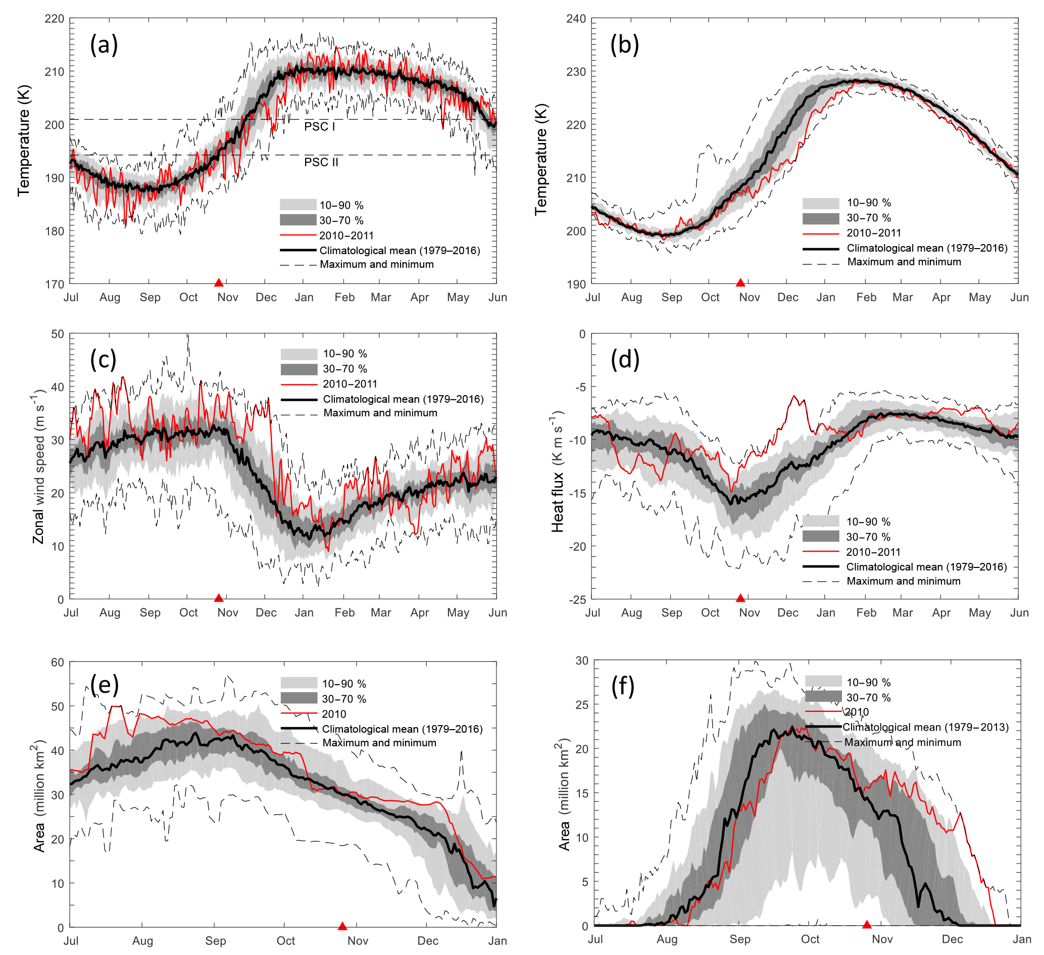
Figure 1 (a) Minimum temperature south of 50^∘ S at 150 hPa; (b) temperature averaged over the polar cap for latitudes south of 60^∘ S at 150 hPa; (c) zonal wind speed at 60^∘ S at 150 hPa; (d) eddy heat flux averaged between 45^∘ S and 75^∘ S for the 45-day period prior to the date indicated at 150 hPa; (e) the area of the polar vortex for 1 July–31 December 2010 on the 460 K isentropic surface; (f) ozone hole area for 1 July–31 December 2010. Temperatures for PSC existence in (a) are determined by assuming a nitric acid concentration of 6 ppbv and a water vapor concentration of 4.5 ppmv. Panels (a)–(f) are based on Modern-Era Retrospective analysis for Research and Applications reanalysis version 2 (MERRA2) data (Bosilovich et al., 2015). The ozone hole area in (f) is determined from OMI ozone satellite measurements (Levelt et al., 2006). The red triangles indicate the time of the Merapi eruption.

Starting with the reconstructed altitude-resolved SO₂ injection time series, the transport of the Merapi plume is simulated for 6 months. The trajectory calculations are driven by the ERA-Interim data (Dee et al., 2011) interpolated on a 1^∘ × 1^∘ horizontal grid on 60 model levels, with the vertical range extending from the surface to 0.1 hPa. The ERA-Interim data are provided at 00:00, 06:00, 12:00 and 18:00 UTC. Outputs of model simulations are given every 3 h at 00:00, 03:00, 06:00, 09:00, 12:00, 15:00, 18:00 and 21:00 UTC. The impact of different meteorological analyses on MPTRAC simulations was assessed by Hoffmann et al. (2016, 2017). In both studies the ERA-Interim data showed good performance.

3 Results

3.1 Meteorological background conditions in Antarctica

The Merapi eruption in 2010 occurred during the seasonal transition from austral spring to summer when the polar vortex typically weakens and the ozone hole shrinks. Figure 1 depicts the meteorological conditions in the polar lower stratosphere (150 hPa, ∼12 km) after the eruption. The minimum temperature south of 50^∘ S (Fig. 1a) was much lower than the climatological mean during mid-November to mid-December but still higher than the low temperature necessary for the existence of PSCs. The polar mean temperature in Fig. 1b, defined as the temperature averaged over latitudes south of 60^∘ S, stayed lower than the climatological mean from November 2010 until February 2011. Corresponding to the low temperatures, the average zonal wind speed at 60^∘ S (Fig. 1c) was significantly larger than the climatological mean value from November 2010 to mid-January 2011. The eddy heat flux in Fig. 1d is the product of meridional wind departures and temperature departures from the respective zonal mean values. A more negative value of the eddy heat flux indicates that wave systems are propagating into the stratosphere and are warming the polar region (Edmon et al., 1980; Newman and Nash, 2000; Newman et al., 2001). There is a strong anticorrelation between temperature and the 45-day average of the eddy heat flux lagged prior to the temperature. Compared with the climatological mean state, the polar vortex was more disturbed during mid-July to the end of August, but from mid-October to late November, the heat flux was much smaller than the long-term average, which meant a reduction in dynamical disturbances. Considering the temperature, the subpolar wind speed and the heat flux, the polar vortex was colder and stronger in November and early December 2010 than it was at the same time in other years (see Fig. 1e). Consistent with the large wind speed and low temperature, the polar vortex was stable after the Merapi eruption until early December 2010. Afterwards, it shrunk abruptly and was destructed by mid-January 2011. In accordance with the strength of the polar vortex, in November and early December 2010 the ozone hole area in Fig. 1f, defined as the region of ozone values below 220 Dobson units (DU) located south of 40^∘ S, was larger than the climatological mean. Meanwhile, the low polar mean temperature and stable polar vortex resulted in a long-lasting ozone hole, which disappeared in the last week of December. The polar vortex broke down by mid-January 2011 when the subpolar wind speed decreased below 15 m s⁻¹ (Fig. 1c).

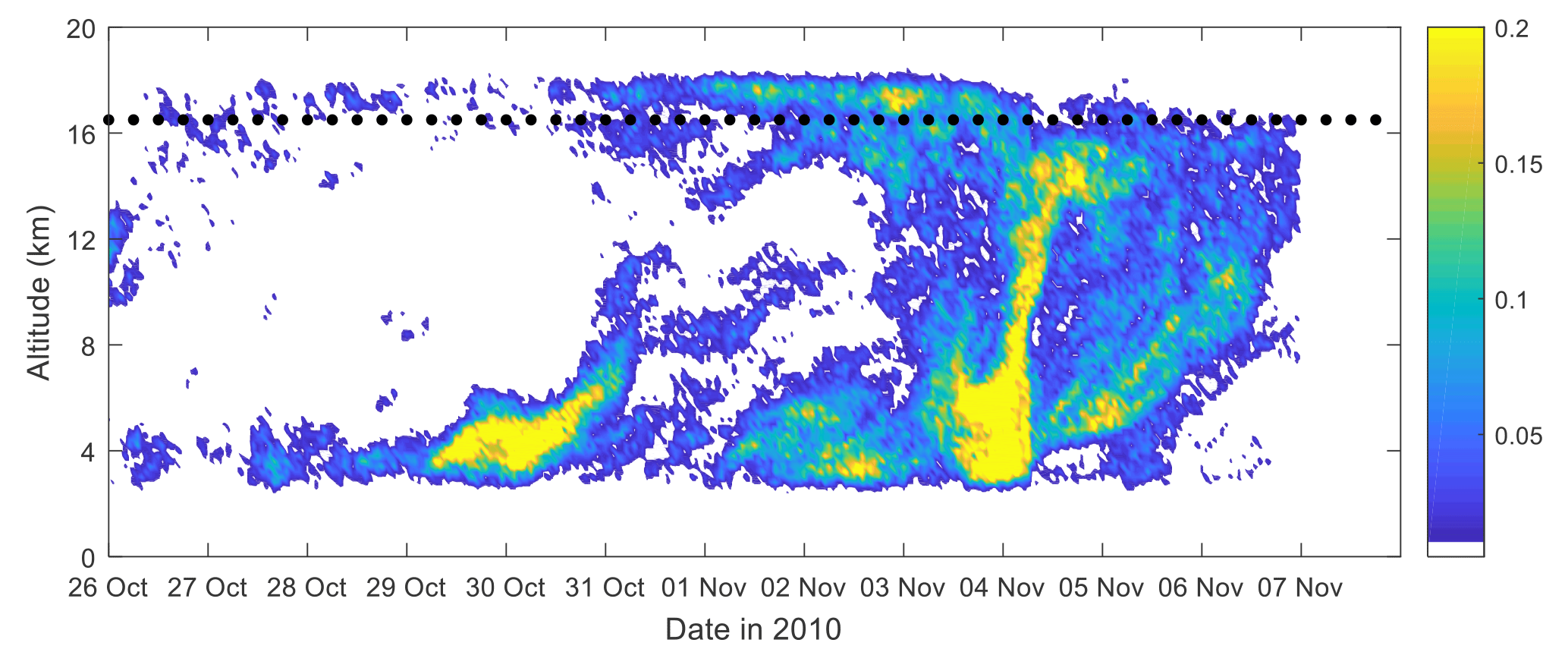
Figure 2 Merapi SO₂ emission time series (unit: kg m⁻¹ s⁻¹) derived from AIRS measurements using a backward trajectory approach (see text for details). The emission data are binned every 1 h and 0.2 km. The ticks for the horizontal axis mark 00:00 UTC on each day. Black dots denote the height of the thermal tropopause (based on the ERA-Interim reanalysis).

3.2 Merapi eruption and SO₂ injection time series

According to the chronology of the Merapi eruption that combined satellite observations from AIRS, the Infrared Atmospheric Sounding Interferometer, the Ozone Monitoring Instrument (OMI) and a limited number of ground-based ultraviolet differential optical absorption spectroscopy measurements (Surono et al., 2012), the explosive eruption first occurred between 10:00 and 12:00 UTC on 26 October and this eruption generated an ash plume that reached 12 km altitude. A period of relatively small explosive eruptions continued from 26 to 31 October. On 3 November, the eruptive intensity increased again accompanied by much stronger degassing and a series of explosions. The intermittent explosive eruptions occurred during 4–5 November, with the climactic eruption on 4 November, producing an ash column that reached up to 17 km altitude. From 6 November, explosive activity decreased slowly and the degassing declined.

Figure 2 shows the time- and altitude-resolved SO₂ injections of the Merapi eruption retrieved using the AIRS SO₂ index data and the backward trajectory approach. It agrees well with the chronology of the Merapi eruption as outlined by Surono et al. (2012). SO₂ was injected into altitudes below 8 km during the initial explosive eruptions on 26–30 October. Starting from 31 October the plume reached up to 12 km. During 1–2 November the SO₂ injections into altitudes below 12 km continued but the mass was less than the mass at the initial phase. On 3 November the intensity increased again and peaked on 4 November. Before 3 November the reconstruction indicates a minor fraction of SO₂ right above the tropopause. The SO₂ above the tropopause is not reported in the study of Surono et al. (2012), but is quite robust in our simulations. Further, CALIOP profiles show that some dust appeared at the height from about 14 to 18 km around Mount Merapi on 2, 3 and 5 November 2010, and between 3 and 17 km on 6 November 2010. It could be a fraction of volcanic plume elevated by the updraft in the convection associated with the tropical storm Anggrek. The center of the tropical storm Anggrek was on the Indian Ocean about 1000 km southwest of Mount Merapi. The SO₂ mass above the tropopause is very small compared with the total SO₂ mass.

To study the long-range transport of the Merapi plume, we initialized 100 000 air parcels as the SO₂ injection time series shown in Fig. 2. A total SO₂ mass of 0.44 Tg is assigned to these air parcels as provided in Surono et al. (2012). Then the trajectories are calculated forward for 6 months. Here, we only considered the plume in the upper troposphere and stratosphere, where the lifetime of both SO₂ and sulfate aerosol is longer than their lifetime in the lower troposphere. Further, the SO₂ was converted into sulfate aerosol within a few weeks (von Glasow et al., 2009; also confirmed by the AIRS SO₂ and MIPAS aerosol data), and we assumed that the sulfate aerosol remained collocated with the SO₂ plume.

Figure 3 shows the evolution of the simulated Merapi plume and compares the plume altitudes to the aerosol top altitudes measured by MIPAS between 7 and 23 November. Immediately after the eruption, the majority of the plume moved towards the southwest and was entrained by the circulation of the tropical storm Anggrek. After Anggrek weakened and dissipated, the majority of the plume parcels in the upper troposphere moved eastward and those in the lower stratosphere moved westward. In general, the altitudes of the simulated plume agree with the MIPAS measurements. The remaining discrepancies of air parcel altitudes being higher than the altitudes of MIPAS aerosol detections can be attributed to the fact that the MIPAS tends to underestimate aerosol top cloud altitudes, which is about 0.9 km in the case of low extinction aerosol layers and can reach down to 4.5 km in the case of broken cloud conditions (Höpfner et al., 2009).

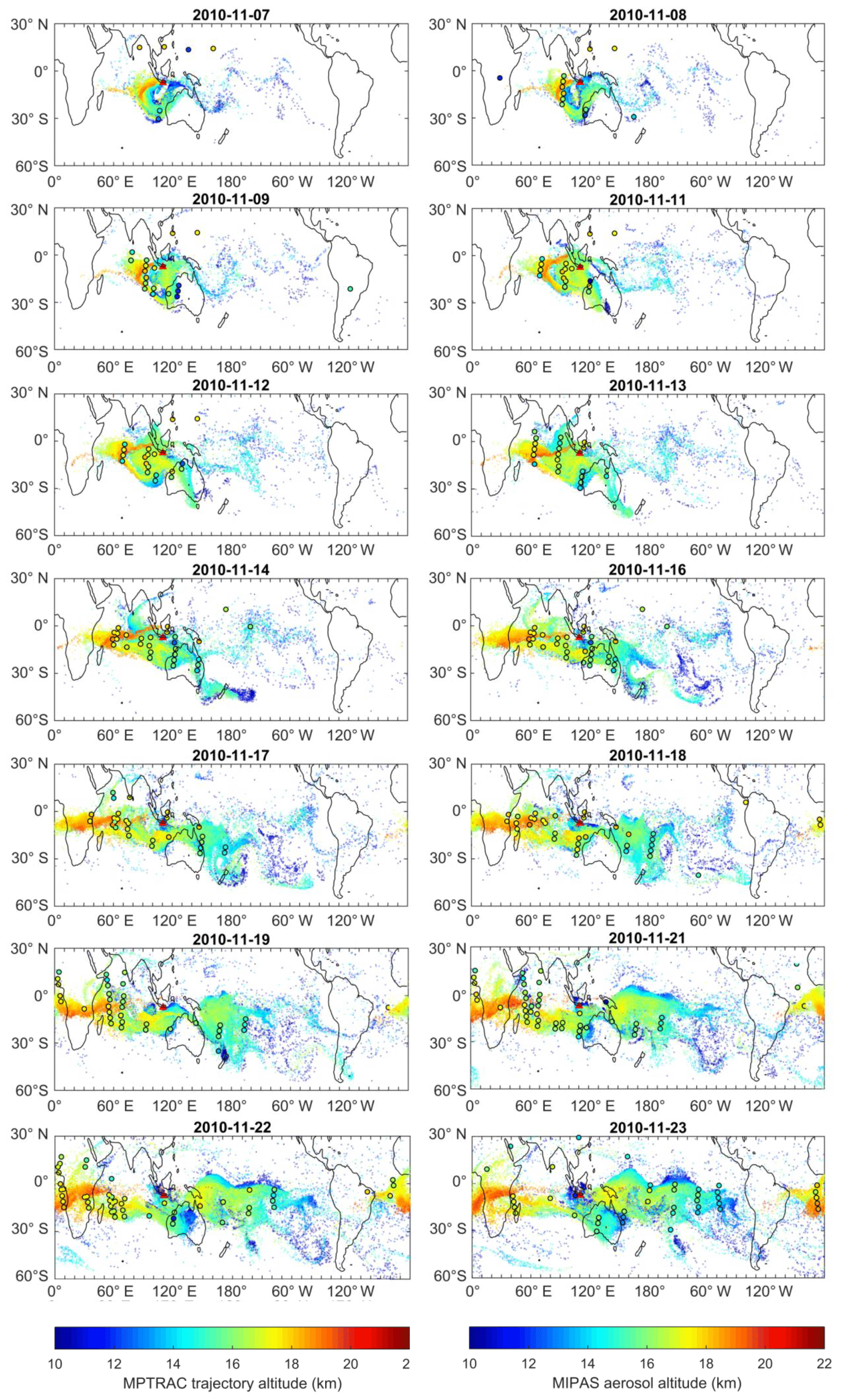
Figure 3 Distribution of the volcanic plume (showing only air parcels higher than 10 km, shading) from MPTRAC simulations (shown for 00:00 UTC on selected days) and MIPAS aerosol detections (ACI < 7) within ±6 h (color-filled circles). The altitudes of all air parcels, regardless of their SO₂ values, are shown. The red triangle denotes the location of Mount Merapi.

Figure 4 Percentage (%) of air parcels in proportion to the total number of air parcels released in the Lagrangian forward simulation, overlaid with monthly mean zonal winds (black contours), the thermal tropopause (black dashed line), the 380 K potential temperature isoline (thick gray dashed line) and 350 and 480 K potential temperature isolines (thin gray dashed lines). Results are binned every 2^∘ in latitude and 1 km in altitude. The red triangle denotes the latitude of Mount Merapi. Please see title of each panel for the time period covered.

3.3 Lagrangian simulation and satellite observation of the transport of the Merapi plume

The early plume evolution until about 1 month after the initial eruption is shown on the maps in Fig. 3 together with MIPAS measurements of volcanic aerosol (only aerosol detections with ACI < 7 are shown). Within about 1 month after the initial eruption, the plume is nearly entirely transported around the globe in the tropics, moving west at altitudes of about 17 km. The lower part of the plume, below about 17 km, is transported southeastward and reaches latitudes south of 30^∘ S by mid-November. The simulated long-term transport of the Merapi plume is illustrated in Fig. 4, showing the proportion of air parcels reaching a latitude–altitude bin every half a month.

Figure 5 Median of MIPAS ACI values between 12 and 18 km (bin size 10 days and 2^∘ in latitude) from January 2005 to April 2012. Only ACI values from 4 to 8 are shown. The red triangle indicates the eruption of Mount Merapi (13). The black filled circles indicate (1) Manam, (2) Soufriere Hills, (3) Tavurvur (Rabaul), (4) Piton de la Fournaise, (5) Jebel at Tair, (6) Chaitén, (7) Kasatochi, (8) Dalaffilla, (9) Australian bushfire, (10) Sarychev Peak, (11) Nyamuragira, (12) Pacaya, (14) Puyehue-Cordón Caulle and (15) Nabro.

The simulation results show that during the first month after the eruption (Fig. 4a–b), the majority of the plume was transported southward roughly along the isentropic surfaces. The significant pathways are above and under the core of the subtropical jet in the Southern Hemisphere. However, because of the transport barrier of the polar jet during austral spring, the plume was confined to the north of 60^∘ S. In December 2010 (Fig. 4c–d), a larger fraction of the plume was transported southward above the subtropical jet core and deep into the polar region south of 60^∘ S as the polar jet broke down. Until the end of January 2011, the majority of the plume entered the midlatitudes and high latitudes in the Southern Hemisphere. Substantial quasi-horizontal poleward transport from the TTL towards the extratropical lowermost stratosphere (LMS) in Antarctica was found from November 2010 to February 2011 (Fig. 4a–h), approximately between 350 and 480 K (∼10–20 km). In March 2011 (Fig. 4i–j), the proportion of the plume that went across 60^∘ S stopped increasing and the maxima of the proportion descended below 380 K. Besides this transport towards Antarctica, a slow upward transport could also be seen. The top of the simulated plume was below the 480 K isentropic surface at around 18 km in Fig. 4a and then the top of the plume went up to 25 km 5 months later in Fig. 4j. This slow upward transport was mainly located in the tropics and can be attributed to the tropical upwelling.

MIPAS ACI values are used to study the plume dispersion and compare with the simulations. Figure 5 displays the time–latitude section of the median value of the MIPAS ACI within the vertical range of 12 and 18 km from January 2005 to April 2012, covering the TTL and the LMS. Only ACI values from 4 to 8 are shown in Fig. 5. The MIPAS data show all the key events that contributed to the aerosol load in the UTLS, i.e., moderate volcanic eruptions from 2005 to 2012 and one large bushfire in 2009, as well as the subsequent dispersion and change of aerosol load over time. The poleward transport of aerosol from the Merapi eruption in 2010, marked by the red triangle in Fig. 5, caused the most long-lasting aerosol signals in the Southern Hemisphere midlatitudes and high latitudes. The small ACI values in the winter months of both hemispheres are attributed to the non-ice PSCs.

While individual aerosol detections can be shown using an ACI < 7 (Fig. 3), we used zonal ACI averages to compare with the simulations. To show the change of aerosol load in the Southern Hemisphere due to the Merapi eruption, we first removed the seasonal cycle from the MIPAS aerosol data. Therefore, we selected a time period from November 2007 to March 2008 with no major SO₂ emission in the Southern Hemisphere UTLS (as shown in Fig. 5) as a “reference state”. We calculated the biweekly median ACI between November 2010 and March 2011 and subtracted it from the biweekly ACI median of the reference state. The results are shown in Fig. 6. Small MIPAS ACI values represent large aerosol load and large ACI values represent small aerosol load, so in Fig. 6, the positive values indicate an increase of the aerosol load and negative values indicate a decrease of the aerosol load. Reference time periods from November 2003 to March 2004 and November 2005 to March 2006 were also tested and they all showed qualitatively comparable results.

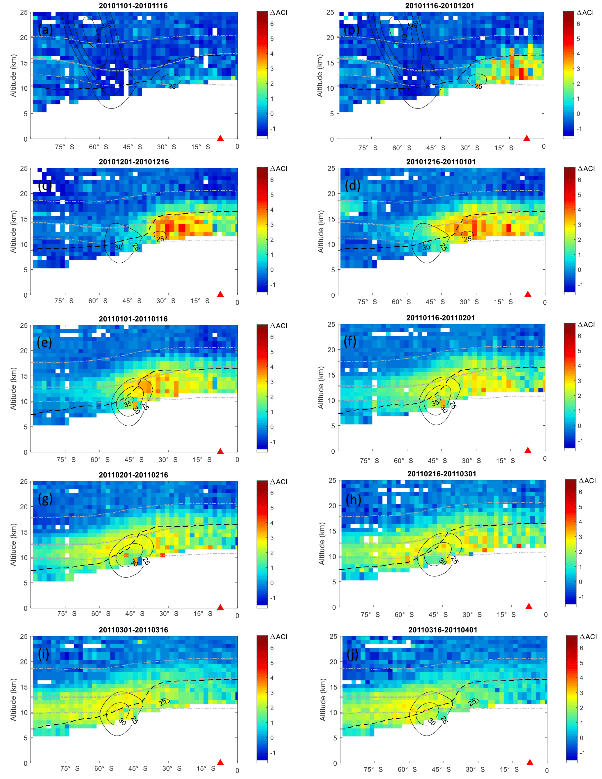
Figure 6 The change of MIPAS ACI values (ΔACI) after the eruption of Merapi in 2010, overlaid with monthly mean zonal winds (black contours), the thermal tropopause (black dashed line), the 380 K potential temperature isoline (thick gray dashed line) and 350 and 480 K potential temperature isolines (thin gray dashed lines). ΔACI values are derived by subtracting the biweekly median ACI between November 2010 and March 2011 from the biweekly median ACI of the reference period between November 2007 and March 2008. Positive values indicate an increase of the aerosol load and negative values indicate a decrease of the aerosol load. Please see the text for details. Results are binned every 2^∘ in latitude and 1 km in altitude. The red triangle denotes the latitude of Mount Merapi. Please see title of each panel for the time period covered.

In the first half of November, the zonal median (Fig. 6a) does not show a signal of the Merapi eruption because during the initial time period, the plume was confined to longitudes around the volcano (see Fig. 3), and the MIPAS tracks did not always sample the maximum concentration, so the median ACI values are large (low concentration or clear air). In the second half of November, the plume was transported zonally around the globe, and hence the largest aerosol increase appeared in the upper troposphere at the latitude of Mount Merapi (Fig. 6b) and then moved quasi-horizontally southward into the UTLS region at ∼30–40^∘ S (Fig. 6c–d), consistent with the simulation result in Fig. 4c–d. The increase of the aerosol load south of 60^∘ S started to become prominent after December 2010, and the poleward movement is most obvious above the 350 K isentropic surface (Fig. 6e–h). The observations confirm the temporal and spatial characteristics of the poleward movement of the aerosol in the simulation in Fig. 4. Later in March 2011, the enhanced aerosol load in the tropics phased out and the aerosol load maxima descended to around the 350 K isentropic surface.

However, the background aerosol level in the tropical upper troposphere and stratosphere is constantly disturbed by tropical and extratropical volcanic eruptions. The reference time period we chose (November 2007 to March 2008) is relatively free of large aerosol sources in the Southern Hemisphere, but the aerosol load in the tropical stratosphere is already elevated by previous volcanic eruptions, e.g., Soufriere Hills (May 2006), Tavurvur (October 2006), Piton de la Fournaise (April 2007) and Jebel at Tair (September 2007). So the change of the aerosol load in Fig. 6 underestimates the increase of aerosol load in the tropical stratosphere after the Merapi eruption. The slow upward transport in the tropics shown in Fig. 4 is about 7 km in 5 months. It is not visible in Fig. 6, but the time series of the MIPAS measurements in the tropical stratosphere reveals a similar upward transport trend (see Fig. A1 in the Appendix).

3.4 Quasi-horizontal transport from the tropics to Antarctica

The MPTRAC simulations and the MIPAS measurements show the transport in the “surf zone” that reaches from the subtropics to high latitudes (Holton et al., 1995), where air masses are affected by both fast meridional transport and the slow BDC. The reconstructed emission time series in Fig. 2 and the MIPAS aerosol measurements in Figs. 3 and 6 show that the volcanic plume was injected into the TTL. Hence, the main transport pathway towards Antarctica is the quasi-horizontal mixing in the lower extratropical stratosphere between 350 and 480 K (see Figs. 4 and 6). Figure 7 illustrates how the volcanic plume between 350 and 480 K approached Antarctica over time. Kunz et al. (2015) derived a climatology of potential vorticity (PV) streamer boundaries on isentropic surfaces between 320 and 500 K using ERA-Interim reanalyses for the time period from 1979 to 2011. This boundary is derived from the maximum product of the meridional PV gradient and zonal wind speed on isentropic surfaces, which identifies a PV contour that best represents the dynamical discontinuity on each isentropic surface. It can be used as an isentropic transport barrier and to determine the isentropic cross-barrier transport related to Rossby wave breaking (Haynes and Shuckburgh, 2000; Kunz et al., 2011a, b). In Fig. 7, gray dashed lines mark PV boundaries on the 350 K isentropic surface. On isentropic surfaces below 380 K, the PV boundaries represent the dynamical discontinuity near the core of the subtropical jet stream. Isentropic transport of air masses across these boundaries indicates exchange between the tropics and extratropics due to Rossby wave breaking. On isentropic surfaces above 400 K, PV boundaries represent a transport barrier in the lower stratosphere, in particular, due to the polar vortices in winter (Kunz et al., 2015). For comparison, we also show the 220 DU contour lines of ozone column density (black isolines in Fig. 7), obtained from OMI on the Aura satellite, indicating the boundary and size of the ozone hole. The PV boundary on 480 K is in most cases collocated with the area of the ozone hole, showing that both quantities provide a consistent representation of the area of the polar vortex.

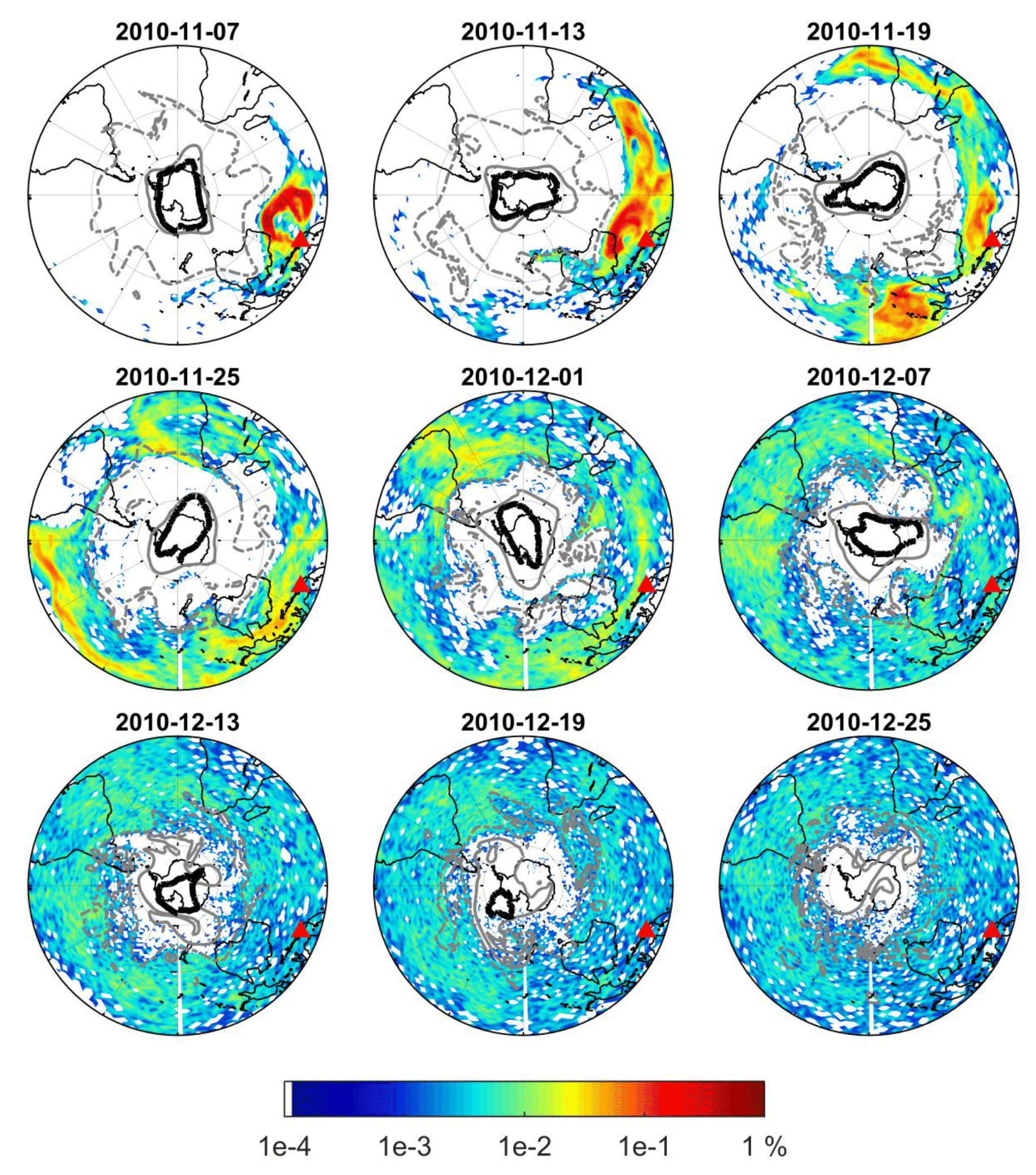
Figure 7 Percentage (%) of air parcels between the isentropic surfaces of 350 and 480 K in proportion to the total number of air parcels released in the Lagrangian forward simulation. All results are at 12:00 UTC on selected dates and binned every 2^∘ in longitude and 1^∘ in latitude. The black contours indicate the 220 DU contour lines of daily mean ozone column density provided by OMI. PV contours marked with gray dashed and solid lines show PV boundaries on the 350 and 480 K isentropic surfaces, respectively (Kunz et al., 2015). The red triangle denotes the location of Mount Merapi.

The Merapi volcanic plume first reached the transport barrier on the 350 K isentropic surface in mid-November and went close to the transport barrier on the 480 K isentropic surface in December. The long-lasting polar vortex prevented the volcanic plume from crossing the transport barrier at 480 K in early December. But from mid-December, the polar vortex became more disturbed and displaced from the South Pole, resulting in a shrinking ozone hole. As mentioned in Sect. 3.1, the ozone hole broke down at the end of December 2010 and the polar vortex broke down by mid-January 2011.

Figure 8 (a) Proportion (%) of the air parcels poleward of the PV-based transport boundaries at the end of each month; (b) proportion (%) of the air parcels south of the geographic latitude of 60^∘ S.

The fractions of the volcanic plume that crosses the individual transport barrier or the latitude of 60^∘ S on each isentropic surface are shown in Fig. 8. In both cases, the proportion increased from November 2010 to January 2011. In November and December 2010 the largest plume transport across the transport barriers occurred between the 360 and 430 K isentropic surface (Fig. 8a), with a peak at 380–390 K. In January and February 2011 the peak was slightly elevated to 390–400 K. In November 2010, the volcanic plume did not cross the 480 K transport barrier of the polar vortex at high altitudes, especially above about 450 K. The high-latitude fraction increased from December 2010 to February 2011 as the weakening of the polar vortex made the transport barrier more permeable. In March and April 2011, the total proportion decreased and the peak descended to 370 K in March and further to 360 K in April. The proportion of the volcanic plume south of 60^∘ S (Fig. 8b) increased slightly from November to December 2010, and then increased significantly from December 2010 to January and February 2011 at all altitudes as the polar vortex displaced and broke down. Finally, the transport to the south of 60^∘ S started to decrease in March 2011. From November 2010 to February 2011 the peak was around 370–400 K, but in March and April 2011 the peak resided around 350–370 K.

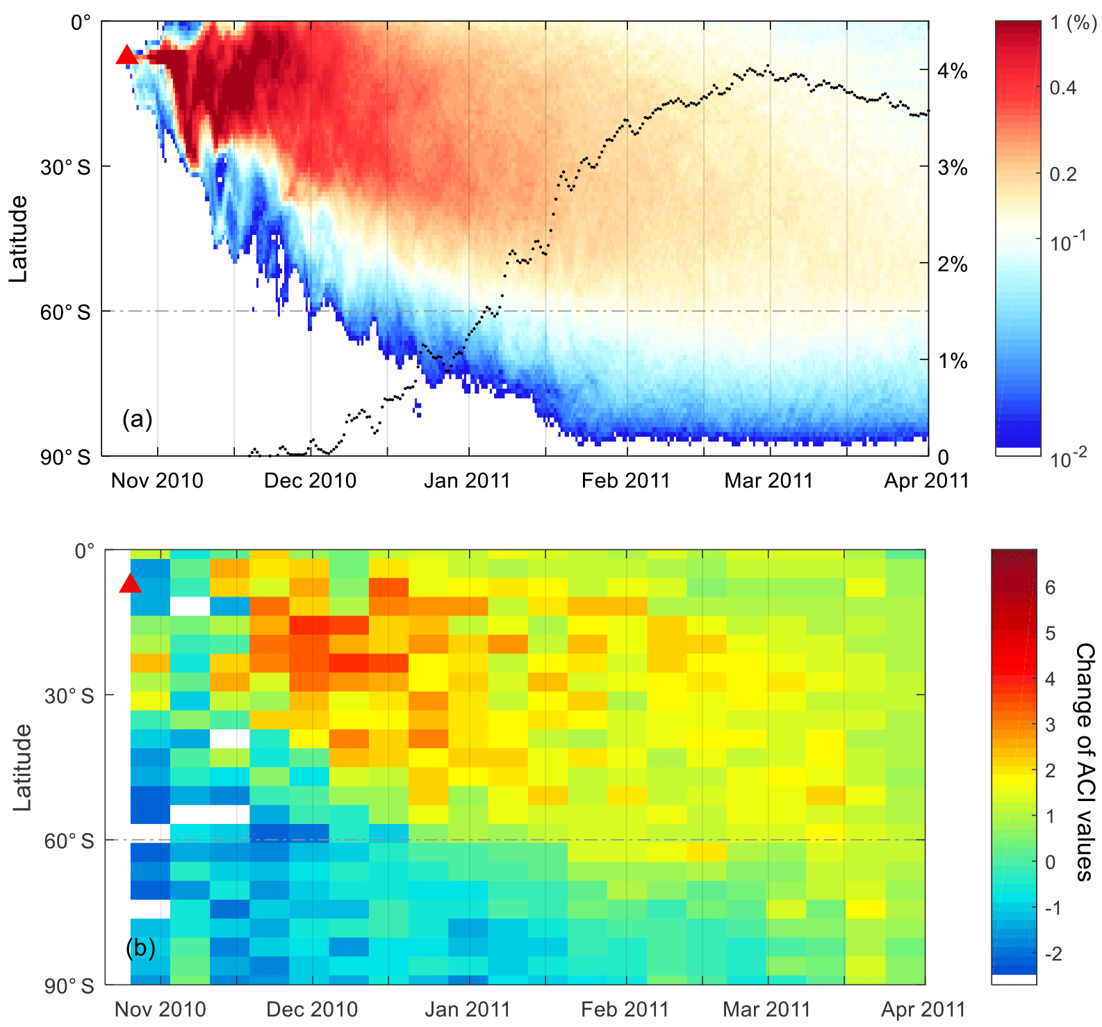
Figure 9 Time and latitude evolution of the (a) percentage (%) of air parcels between the isentropic surfaces of 350 and 480 K from the Lagrangian simulations (shading, only percentages larger than 0.05 % are shown; bin size: 12 h and 1^∘ in latitude) and the proportion (%) of air parcels south of 60^∘ S (black dots); (b) the change of MIPAS ACI values (ΔACI) after the eruption of Merapi in 2010 between 350 and 480 K. ΔACI values are derived by subtracting the biweekly median ACI between November 2010 and March 2011 from the biweekly median ACI of the reference period between November 2007 and March 2008. Positive values indicate an increase and negative values indicate a decrease of the aerosol load (bin size: 8 days and 4^∘ in latitude). Please see the text for details. The red triangle denotes the time and latitude of the Merapi eruption.

Figure 9a summarizes the simulated poleward transport of the volcanic plume between the isentropic surfaces of 350 and 480 K from November 2010 to March 2011 and the percentage of air parcels south of 60^∘ S. The percentage was calculated by dividing the number of SO₂ parcels between 350 and 480 K south of 60^∘ S by the total number of SO₂ parcels released for the forward trajectory simulation. Figure 9b demonstrates the change of aerosol load in the same vertical range for MIPAS aerosol detections. As in Sect. 3.3, we calculated the median ACI between November 2010 and March 2011 and subtracted it from the ACI median of the reference state between November 2007 and March 2008. Positive values indicate an increase of the aerosol load and negative values indicate a decrease of the aerosol load. The simulations show that the plume reached 60^∘ S in December 2010. Correspondingly, the aerosol load south of 60^∘ S was elevated. The percentage fluctuated, but increased until the end of February 2011, with a maximum percentage of about 4 %. A steep increase occurred from mid-December 2010 to the end of January 2011, following the displacement and breakdown of the polar vortex. The elevated aerosol load south of 60^∘ S decreased from March 2011, and part of the plume descended to altitudes below 350 K as shown by Fig. 8b. The MIPAS aerosol measurements in Fig. 9b, where a positive ACI difference indicates an increase in the aerosol load, confirm the simulated transport pattern in Fig. 9a. Overall, simulations and observations indicate the largest increase of the aerosol load in the tropics and midlatitudes, but also show a significant enhancement over the south polar region after December 2010.

4 Discussion

The results presented in Sect. 3 show that the main transport pathway for the poleward transport of the Merapi volcanic plume to Antarctica was between the isentropic surfaces of 350 and 480 K (about 10 to 20 km), covering the TTL and the lower stratosphere at midlatitudes and high latitudes. Our findings using the MPTRAC model and MIPAS ACI are supported by the sulfate aerosol volume density retrievals by Günther et al. (2018). The aerosol enhancement due to volcanic eruptions between 12 and 18 km revealed in Fig. 5 agrees with the sulfate aerosol enhancement shown in Fig. 5 in Günther et al. (2018). Figure 5 in Günther et al. (2018) shows that after the eruption of Merapi in 2010, clear poleward dispersion of sulfate aerosol can be seen between 12 and 18 km, and the most prominent signal appears at 14 and 16 km. The sulfate aerosol mole fraction south of 60^∘ S increased also from the end of December 2010 as shown in our Fig. 9, although the specific date is not clear because of the seasonal cycle in the data. The enhanced sulfate aerosol lasted until the middle of March 2011 at 12 and 14 km, and until early April at 16 km, which also generally agrees with our results.

There are some differences in the MIPAS ACI data used in this study and the sulfate aerosol retrievals in Günther et al. (2018), which may result in some minor discrepancies regarding the spatial distribution of aerosols. The MIPAS ACI data in this study are given on a 1.5 km vertical sampling grid in the UTLS region, but the sulfate aerosol retrieval in Günther et al. (2018) had a vertical resolution of 3–4 km. And comparing with the MIPAS ACI, there are further steps in Günther et al. (2018) to deal with ice cloud and to filter out PSCs. Due to the vertical resolution of 3–4 km, once ice cloud is detected, Günther et al. (2018) removed all retrieved data up to 4 km above the ice cloud. And they filtered out PSCs based on latitude, time and temperature criteria; i.e., if the temperature between 17 and 23 km dropped below the nitric acid trihydrate existence temperature (195 K) poleward of 40^∘ in the Northern Hemisphere winter (15 November to 15 April) and the Southern Hemisphere winter (1 April to 30 November), the retrieval results were discarded. Filtering out PSCs based on time, latitude and temperature criteria may lead to a loss of clear air profiles, e.g., when the synoptic temperature is sufficiently low but no PSCs are present. Usually the PSCs signals are much stronger than the aerosol signals, so we keep the non-ice PSC data to give an impression of the time and region when and where the identification of volcanic aerosol is not possible.

Based on the simulation results in Sect. 3.4, up to 4 % of the volcanic plume air parcels were transported from the TTL to the lower stratosphere in the south polar region till the end of February 2011. We assigned a total mass of 0.44 Tg to all SO₂ parcels released, which means the Merapi eruption contributed about 8800 t of sulfur to the polar lower stratosphere within 4 months after the eruption, assuming that the sulfate aerosol converted from the SO₂ remained in the plume. The MPTRAC model we used to simulate the three-dimensional movement of air parcels in the volcanic plumes can estimate the conversion of SO₂ to sulfate aerosol during the transport process; however, it does not resolve the chemical processes of aerosol formation. Hence, the estimated 8800 t of sulfur is the maximum value since processes as, e.g., wet deposition remove sulfur from the atmosphere. But in the lower stratosphere, the atmosphere is relatively dry and clean compared with the lower troposphere, so the sulfate aerosol has a lower possibility of interacting with clouds or of being washed out. In fact, in the polar lower stratosphere, usually sedimentation and downward transport by the BDC are the main removal processes. Clouds and washout processes usually cannot be expected in the lower stratosphere. However, the amount of sulfate aerosol in the plume could also be affected by other mechanisms that speed up the loss of sulfur, for example, coagulation in the volcanic plume, or the absorption of sulfur onto fine ash particles. But for the moderate eruption of Merapi in 2010, sulfuric particle growth may not be as significant as it is in a large volcanic eruption, so the scavenging efficiency of sulfur will be low. So generally, our estimation may be larger than the actual value, but this number may be considered as the upper limit of the contribution of the Merapi eruption.

Besides, a kinematic trajectory model like MPTRAC, in which reanalysis vertical wind is used as vertical velocity, typically shows higher vertical dispersion in the equatorial lower stratosphere compared with a diabatic trajectory model (Schoeberl et al., 2003; Wohltmann and Rex, 2008; Liu et al., 2010; Ploeger et al., 2010, 2011). However, the ERA-Interim reanalysis data used in this study to drive the model may constrain the vertical dispersion much better than older reanalyses (Liu et al., 2010; Hoffmann et al., 2017). The meridional transport in this study was mainly quasi-horizontal transport in the midlatitude and high-latitude UTLS region, so the effect of the vertical speed scheme is limited.

The aerosol transported to the polar lower stratosphere will finally descend with the downward flow and have a chance to become a nonlocal source of sulfur for Antarctica through dry and wet deposition, following the general precipitation patterns. Quantifying the sulfur deposition flux onto Antarctica is beyond the scope of this study, though. Model results of Solomon et al. (2016) suggest that the Merapi eruption made a small but significant contribution to the ozone depletion in the following year over Antarctica in the vertical range of 100–200 hPa, roughly between 10 and 14 km. This altitude range is in agreement with our results; we found transport into the Antarctic stratosphere between 10 and 20 km. When the volcanic plume was transported to Antarctica in December 2010, the polar synoptic temperature at these low height levels was already too high for the formation of PSCs. The additional ozone depletion found by Solomon et al. (2016), together with the fact that sulfate aerosol was transported from Merapi into the Antarctic stratosphere between November and February where no PSCs are present during polar summer, may support the study that suggested that significant ozone depletion can also occur on cold binary aerosol (Drdla and Müller, 2012). The Merapi eruption in 2010 could be an interesting case study for more sophisticated geophysical models to study the aftermath of volcanic eruptions on polar processes.

5 Summary

In this study, we analyzed the poleward transport of volcanic aerosol released by the Merapi eruption in 2010 from the tropics to the Antarctic lower stratosphere. The analysis was based on AIRS SO₂ measurements, MIPAS sulfate aerosol detections and MPTRAC transport simulations. First, we estimated altitude-resolved SO₂ injection time series during the explosive eruption period using AIRS data together with a backward trajectory approach. Second, the long-range transport of the volcanic plume from the initial eruption to April 2011 was simulated based on the derived SO₂ injection time series. Then the evolution and the poleward migration of the volcanic plume were analyzed using the forward trajectory simulations and MIPAS aerosol measurements. The simulations are compared with and verified by the MIPAS aerosol measurements.

Results of this study suggest that the volcanic plume from the Merapi eruption was transported from the tropics to the south of 60^∘ S within a timescale of 1 month. Later on, in the UTLS region a fraction of the volcanic plume (∼4 %) crossed 60^∘ S, even further to Antarctica until the end of February 2011. As a result, the aerosol load in the Antarctic lower stratosphere was significantly elevated. This relatively fast meridional transport of volcanic aerosol was mainly carried out by quasi-horizontal mixing from the TTL to the extratropical lower stratosphere. Based on the simulations, most of the quasi-horizontal mixing occurred between the isentropic surfaces of 360 to 430 K. This transport was in turn facilitated by the weakening of the subtropical jet and the breakdown of the polar vortex in the seasonal transition from austral spring to summer. The polar vortex in late austral spring 2010 was relatively strong compared to the climatological mean state. However, in December 2010 the polar vortex was displaced off the South Pole and later on broke down when the plume went to the high latitudes, so the volcanic plume did not penetrate the polar vortex but entered the South Pole with the breakdown of the polar vortex.

Overall, after the Merapi eruption, the largest increase of aerosol load occurred in the Southern Hemisphere midlatitudes, and a relatively small but significant fraction of the volcanic plume (4 %) was further transported to the Antarctic lower stratosphere within 4 months after the eruption. As a maximum estimation, it contributed up to 8800 t of sulfur to the Antarctic stratosphere, which indicates that long-range transport under favorable meteorological conditions can make moderate tropical volcanic eruptions an important remote source of sulfur to Antarctica.

Appendix A

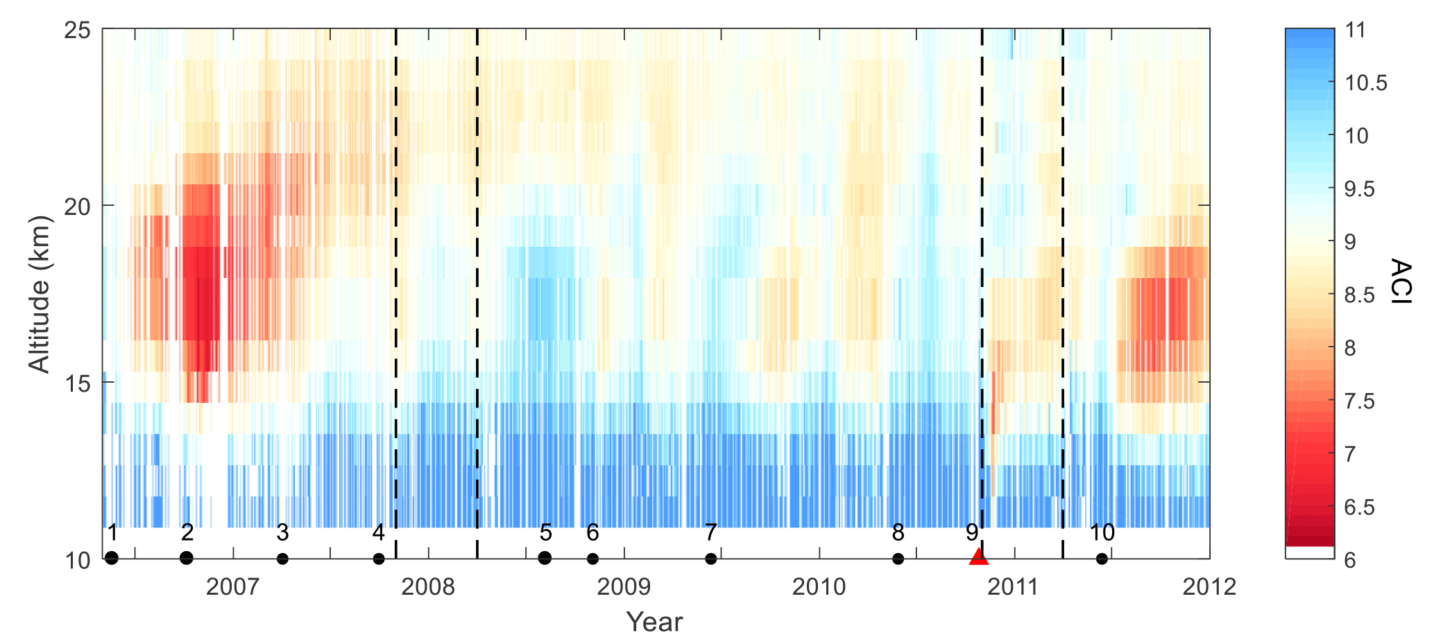
Figure A1 MIPAS 9-day running median of ACI between 10^∘ N and 10^∘ S from May 2006 to December 2011. The dashed vertical lines indicate the reference state from November 2007 to March 2008, and the investigation period for the Merapi eruption from November 2010 to March 2011. The red triangle indicates the time of the Merapi eruption (9). The black dots indicate (1) Soufriere Hills, (2) Tavurvur (Rabaul), (3) Piton de la Fournaise, (4) Jebel at Tair, (5) Kasatochi, (6) Dalaffilla, (7) Sarychev, (8) Pacaya and (10) Nabro.

Figure A1 shows the 9-day running median values of the MIPAS ACI between 10^∘ N and 10^∘ S. During the time period of the reference state (November 2007 to March 2008), the aerosol load in the tropical stratosphere from 20 to 25 km is elevated by a couple of previous volcanic eruptions. The aerosol load at this vertical range after the Merapi eruption in 2010 is apparently smaller compared with the reference state.

It should be noted that there are semiannual data oscillations in the MIPAS ACI aerosol detections. This periodic pattern is caused by the aerosol index that uses the atmospheric window region between 960 and 961 cm⁻¹. Around this window region, there are CO₂ laser bands. Due to the semiannual temperature changes at about 50 km (semiannual oscillation), the CO₂ radiance contribution to this window region also oscillates. As this window is generally very clear of other trace gases, this oscillation is not only visible at higher altitudes but also in the lower stratosphere because the satellite line of sight looks through the whole layer (Wu et al., 2017). But even though with the semiannual data oscillations, the upward transport of the aerosol from the Merapi eruption in the tropical stratosphere is still visible, the vertical speed is estimated to be about 7–8 km in 5 months (November 2010 to March 2011).