the Creative Commons Attribution 4.0 License.
the Creative Commons Attribution 4.0 License.
 | 23 Oct 2018
Uncertainty of atmospheric microwave absorption model: impact on ground-based radiometer simulations and retrievals
Domenico Cimini
Philip W. Rosenkranz
Mikhail Y. Tretyakov
Maksim A. Koshelev
Filomena Romano
This paper presents a general approach to quantify absorption model uncertainty due to uncertainty in the underlying spectroscopic parameters. The approach is applied to a widely used microwave absorption model (Rosenkranz, 2017) and radiative transfer calculations in the 20–60 GHz range, which are commonly exploited for atmospheric sounding by microwave radiometer (MWR). The approach, however, is not limited to any frequency range, observing geometry, or particular instrument. In the considered frequency range, relevant uncertainties come from water vapor and oxygen spectroscopic parameters. The uncertainty of the following parameters is found to dominate: (for water vapor) self- and foreign-continuum absorption coefficients, line broadening by dry air, line intensity, the temperature-dependence exponent for foreign-continuum absorption, and the line shift-to-broadening ratio; (for oxygen) line intensity, line broadening by dry air, line mixing, the temperature-dependence exponent for broadening, zero-frequency line broadening in air, and the temperature-dependence coefficient for line mixing. The full uncertainty covariance matrix is then computed for the set of spectroscopic parameters with significant impact. The impact of the spectroscopic parameter uncertainty covariance matrix on simulated downwelling microwave brightness temperatures (TB) in the 20–60 GHz range is calculated for six atmospheric climatology conditions. The uncertainty contribution to simulated TB ranges from 0.30 K (subarctic winter) to 0.92 K (tropical) at 22.2 GHz and from 2.73 K (tropical) to 3.31 K (subarctic winter) at 52.28 GHz. The uncertainty contribution is nearly zero at 55–60 GHz frequencies. Finally, the impact of spectroscopic parameter uncertainty on ground-based MWR retrievals of temperature and humidity profiles is discussed.
- Article
(2556 KB) - Full-text XML
-
Supplement
(132 KB) - BibTeX
- EndNote


Atmospheric absorption models are used to simulate the absorption and emission of electromagnetic radiation by atmospheric constituents. Atmospheric absorption models are thus crucial to compute radiative transfer through the atmosphere (Mätzler, 1997; Saunders et al., 1999; Clough et al., 2005; Buehler et al., 2005; Eriksson et al., 2011), which is needed to simulate and validate passive and active remote sensing observations, such as those from microwave radiometer (MWR) and radar instruments (Hewison et al., 2006; Maschwitz et al., 2013). Absorption and radiative transfer models, representing the forward operator for atmospheric radiometric applications, are also exploited in physical approaches for the solution of the inverse problem, i.e., the retrieval of atmospheric parameters from remote sensing radiometric observations (Westwater, 1978; Rodgers, 2000; Rosenkranz, 2001; Rosenkranz and Barnet, 2006; Cimini et al., 2010). Thus, absorption and radiative transfer models, and their uncertainty, have general implications for atmospheric sciences, including meteorology and climate studies.
Comparisons of different radiative transfer and microwave absorption models have been performed to quantify the difference in calculated brightness temperatures (TB) and the agreement with ground-based, satellite, shipborne, and airborne radiometric observations (Westwater et al., 2003; Melsheimer et al., 2005; Hewison, 2006a; Hewison et al., 2006; Brogniez et al., 2016). However, the uncertainty affecting current microwave radiometric observations is often comparable to the differences in radiative transfer calculations, and thus clear and definite answers were not always obtainable.
Absorption models are based on quantum mechanics theory and rely on parameterized equations to compute atmospheric absorption given the thermodynamic conditions and abundance of constituents (Rosenkranz, 1993). The spectroscopic parameters entering the parameterized equations are determined through theoretical calculations or laboratory and field measurements, and their values are continuously refined (Liebe et al., 1989; Rosenkranz, 1998; Liljegren et al., 2005; Turner et al., 2009; Mlawer et al., 2012; Koshelev et al., 2018). Review papers are published occasionally to summarize the proposed modifications (Rothman et al., 2005, 2013; Gordon et al., 2017). The absorption models described in Rosenkranz (1998, 2017) are cited frequently in this paper and are hereafter called R98 and R17, respectively. The review by Tretyakov (2016) is also cited frequently, meaning Tretyakov (2016) and the references therein.
The uncertainty affecting the values of spectroscopic parameters contributes to the uncertainty of the simulated absorption, which in turn affects atmospheric radiative transfer calculations. Thus, the uncertainty affecting spectroscopic parameters contributes to the uncertainty of simulated remote sensing observations and consequently to the uncertainty of remote sensing retrievals of atmospheric thermodynamic and composition profiles (Boukabara et al., 2005a; Verdes et al., 2005). This situation does not apply to microwave radiometry only, but is general to all wavelength regions (Long and Hodges, 2012; Alvarado et al., 2013, 2015; Connor et al., 2016). However, it must be considered that the uncertainty affecting different spectroscopic parameters may be correlated. Therefore, in addition to the uncertainty affecting the single parameters, the full uncertainty covariance matrix should be estimated to account for the correlation in radiative transfer calculations and retrievals (Rosenkranz, 2005; Boukabara et al., 2005b).
In the last decade, the Global Climate Observing System (GCOS) Reference Upper-Air Network (GRUAN) has evolved from aspiration to reality (Bodeker et al., 2015). GRUAN is now delivering reference-quality measurement of essential climate variables (ECVs), for which the uncertainty contributions are carefully evaluated. In addition to radiosonde observations (Dirksen et al., 2014), ground-based remote sensing products are planned in GRUAN, including from microwave radiometer (MWR) profilers. Most common ground-based MWR profilers operate in the 20–60 GHz range to infer ECVs such as tropospheric temperature and water vapor profiles and vertically integrated water vapor and liquid water contents. MWR adds value to GRUAN by providing redundant measurements with respect to radiosondes, but covering the complete diurnal cycle at high (e.g., 1 min) temporal resolution. The various sources of uncertainty for MWR retrievals have been reviewed in the framework of the GRUAN-related GAIA-CLIM project (http://gaia-clim.eu/, last access: 1 May 2018, Thorne et al., 2017). One such source is the spectroscopic parameter uncertainty, which appears to be the least investigated among all (Maschwitz et al., 2013; GAIA-CLIM, Gaps Assessment and Impacts Document (GAID) – G2.37, 2017). The premises above call for a thorough investigation of the uncertainty affecting spectroscopic parameters entering current microwave absorption models and their impact on MWR simulated observations and retrievals. Focusing primarily on clear-sky retrievals, the main constituents contributing to atmospheric microwave absorption in the 20–60 GHz range are water vapor and oxygen.
Thus, the main purpose of this paper is to introduce a rigorous approach for quantifying the absorption model uncertainty. Although the approach is general and not limited to any particular instrument, observing technique, or frequency range, we demonstrate its use through the application to ground-based microwave radiometer simulations and retrievals. The analysis thus consists of the following four steps:
-
review recent work concerning water vapor and oxygen spectroscopic parameters and their associated uncertainties;
-
perform a sensitivity study to investigate the dominant uncertainty contribution to radiative transfer calculations;
-
estimate the full uncertainty covariance matrix for the dominant parameters; and
-
propagate the uncertainty covariance matrix to estimate the impact on MWR simulated observations and atmospheric retrievals.
Thus, the paper is organized as follows: Sect. 2 summarizes the equations used in the considered microwave absorption model and defines their parameters. Section 3 presents the results of the uncertainty sensitivity study. Section 4 discusses the approach to estimate the uncertainty covariance matrix. Section 5 presents the impact of spectroscopic uncertainty on simulated downwelling 20–60 GHz TB and on the associated ground-based atmospheric temperature and humidity profile retrievals. Section 6 presents a summary, main conclusions, and hints for future work. Finally, the Appendix reviews recent updates to spectroscopic parameters in the considered microwave absorption models.
Absorption happens when radiation travels through a dissipative medium. The radiation intensity as a function of the path length l through the medium is given by the Beer–Lambert–Bouguer law, , in which I0 is the incident radiation intensity, I is the transmitted radiation intensity passed through the medium, and α is the absorption coefficient of the medium, which depends on the radiation frequency ν. The absorption coefficient is a macroscopic parameter that represents the interaction of incident electromagnetic energy with the constituent molecules. Here we consider atmospheric absorption, and thus α(ν) represents the absorption spectrum of the gas mixture forming the atmosphere. The gas absorption spectrum is the sum of two components: the resonant and nonresonant absorption. The resonant absorption is a property of individual molecules; it occurs at certain frequencies (absorption lines) associated, for example, with the change in the angular momentum of the molecule (rotational transition) or the oscillation frequency (vibrational transition). Nonresonant absorption arises from the interaction of molecules with each other, i.e., due to the nonideality of gas. Thus, the gas absorption coefficient can be expressed as the sum of the resonance lines and the nonresonance absorption:
The following sections describe the resonant and nonresonant absorption components and the parameterization as defined in the family of absorption models considered here, i.e., R98 and R17 as well as others introduced in Sect. 2.4. Therefore, the review presented here applies specifically to this family of models. However, the approach presented in this paper can be considered generally valid for any absorption model.
2.1 Resonant absorption
Resonant absorption is modeled by computing the contribution of each significant absorption line (line by line). Following Rosenkranz (1993), the power absorption coefficient at frequency ν for a specified molecular species with n molecules per unit volume is given by
where
is the line-shape function, while the following line parameters refer to the ith absorption line of the specified molecule: the center frequency (νi), the half-width at half amplitude (Δνi), the integrated intensity at temperature T (Si(T)), and the mixing parameter (Yi). Note that the summation in Eq. (2) only includes i > 0, as negative resonances are included in the line-shape function, and the zero-frequency transition (Debye absorption, which must be taken into account in molecular oxygen), sometimes referred as to i=0, is treated below. The line-shape function Eq. (3) considers the fact that in the case of two or more lines contributing significantly to the absorption, there may be non-negligible line mixing, in which case the resulting intensity of the band cannot be calculated as a simple sum of isolated line profiles. Instead, the line-mixing coefficients Yi account for the line-mixing effect in the first-order (in pressure) approximation suggested by Rosenkranz (1975). A second-order expansion was later proposed by Smith (1981), adding coefficients accounting for the mixing of line intensities and shifting of line central frequencies.
In the frequency range considered here (20–60 GHz), the line-mixing effect is fundamental for understanding oxygen absorption, while it is negligible for water vapor (Yi≅0) (Ma et al., 2014). Then for water vapor, the line-shape function reduces to the van Vleck–Weisskopf profile:
The van Vleck–Weisskopf profile was demonstrated to fit experimental data well on the 22 GHz line (Hill, 1986) and 183 GHz line (see Fig. 5 and related references from Tretyakov, 2016); also, Koshelev et al. (2018) found that speed-dependence effects amount to less than 1 % deviation with respect to the van Vleck–Weisskopf profile near 22 GHz.
The van Vleck–Weisskopf profile can also be used for taking into account zero-frequency transitions by letting ν0=0 (Van Vleck, 1947). All these transitions overlap each other and can be treated as a single resonance line. This line in O2 may be included in the summation of Eq. (2) as i=0, with ν0=0, Y0=0. However, a different definition of line intensity must be used:
which has a finite nonzero value as ν0→0. Thus, introducing γ0 as the O2 zero-line half-width at half amplitude, this absorption reduces to the following expression, which has the Debye line-shape factor (Rosenkranz, 1993):
Note that the line profiles (3, 4, 6) are valid only when the frequency detuning satisfies , where τc is the finite duration of molecular collision. Therefore, a way to model the line absorption is the so-called line wing cutoff, i.e., assuming zero absorption at detunings larger than a cutoff frequency. The value of the cutoff frequency proposed by Clough et al. (1989), 750 GHz, is widely accepted and used in some absorption models (R98; Clough et al., 2005). It should also be mentioned that line profiles (3, 4, 6) take into account only the collisional broadening mechanism and ignore additional line broadening related to thermal molecular movement (Doppler broadening), which has a significant effect in the considered frequency range only at very low gas densities (i.e., altitudes above 60 km). Fine effects of collisional narrowing of the resonance line, due to speed dependence of absorbing molecule cross section or velocity-changing collisions, are also ignored.
2.2 Nonresonant absorption
Nonresonant absorption accounts for the absorption characterized by the smooth frequency dependence remaining after considering the effect of resonant lines. The mechanism for nonresonant absorption arises from the nonideality of atmospheric gases and corresponds to the absorption by collisionally interacting molecules. At usual atmospheric conditions only pair interaction is significant. This interaction during a finite time of collision may lead to significant (either positive or negative) deviation of resonance line far wings from the absorption calculated using profiles (3–6). For each molecule, the sum of these deviations over all lines gives absorption smoothly varying with frequency. Another component of nonresonance absorption corresponds to molecular pairs (bimolecular absorption). The latter can be further subdivided into three parts corresponding to free molecular pairs, quasi-bound (metastable) dimers, and true-bound (stable) dimers. All these absorption contributions also vary very smoothly with frequency at atmospheric conditions due to either the short lifetime of bimolecular state (free pairs and quasi-bound dimers) or an extremely dense and collisionally broadened spectrum of loosely bound molecular pairs (quasi-bound dimers and true-bound dimers).
To model nonresonance bimolecular absorption in the atmosphere, it should be taken into account that pair interactions occur in any atmospheric gases and their mixtures. For convenience, the treatment of atmospheric nonresonance absorption is divided in two contributions, one deriving from dry air and the other from water vapor.
The dry contribution is due to the interaction of dry air molecules with each other. Only molecular nitrogen and oxygen are considered, as they account for nearly 100 % of the atmospheric mixture and absorption. Because of the dominant nitrogen contribution this component can be approximately calculated in the considered frequency range as
where is the absorption due to N2–N2 interactions and ε(νT) accounts for the absorption due to O2–O2 and N2–O2 interactions, considering N2 and O2 relative abundances and absorption intensities (Boissoles et al., 2003).
Concerning the water vapor contribution to nonresonance absorption, despite a general understanding of the physical nature (e.g., Shine et al., 2012; Tretyakov et al., 2014; Serov et al., 2017), there are no sufficiently accurate theoretical models for calculating the spectra of all necessary components (especially in gas mixtures) and their temperature dependences. Therefore, for practical purposes parameters of the observed nonresonant absorption are determined using simple empirical models, which have not been supported by accurate theoretical calculations and are based on experimental data only (Tretyakov, 2016). The so-called continuum absorption is thus empirically defined as the difference between the total observed absorption and the calculated contribution of resonance lines:
Note that in such a definition the resulting continuum absorption contains the nonresonant absorption as well as the unknown contribution from resonance line far wings at frequency detunings exceeding the somewhat arbitrary cutoff frequency introduced above.
2.3 Absorption model parameterization
The spectroscopic parameters appearing in the above equations may depend on temperature (T) and pressure (P). Most experimental data on spectroscopic parameters are obtained near room temperature, and thus tabulated values are available at reference temperature T0 (usually 296 or 300 K). Parametric functions are used to express the dependence on T and P in common absorption models.
For the line intensity, the temperature dependence is given by the total number of populated molecular states (the partition sum), which can be calculated numerically (Gamache et al., 2017), and the population of molecular energy levels corresponding to the transition. The latter is calculated from the energy of the lower level and the frequency of the corresponding transition. Thus, calling k the Boltzmann constant, Elow the energy of the lower level, S(T0) the intensity at the reference temperature T0, and introducing the so-called inverse temperature (), the intensity is written as (Rosenkranz, 1993)
where the temperature exponent nS accounts for the temperature dependence of the partition sum and differs for asymmetric (e.g., water vapor, nS≅2.5) and linear (e.g., oxygen, nS≅2.0) molecules.
For pressure-broadened line coefficients, it is convenient to introduce normalized coefficients relative to the reference temperature T0 and independent of pressure. In general, experimental studies fit them to a function of the form γ=γ(T0) θn P, where γ(T0) and n are constant coefficients. The power function is generally suitable for atmospheric applications to account for the temperature dependence of the above parameters as it works well within ±50 K from T0.
For water vapor absorption, the line width and the line center frequency are differently affected in the case of broadening induced by water vapor (self-broadening, indicated by s) or by dry air (foreign broadening, indicated by a). Thus, calling Pw and Pd the partial pressures of water vapor and dry air and the “zero pressure” transition frequency of the ith absorption line, line broadening and shifting are written respectively as
where γi,s, γi,a and δi,s, δi,a are the self and foreign parameters for broadening and shifting, respectively, at the reference temperature T0, and , , , and are the temperature exponents for line self-broadening, foreign broadening, self-shifting, and foreign shifting. In R17, the ratio of shift to broadening (Ri) is used as a parameter instead of the shifting parameter, e.g., . This implicitly assigns the same temperature dependence to broadening and shifting, which is done because of the absence of relevant measurements for nδ, although theory suggests that it could differ from nγ (Pickett, 1980).
Similarly, for oxygen it is convenient to introduce normalized broadening (γi) and mixing (yi) coefficients. In addition, the water-to-air broadening (rw2a) and mixing () ratios are introduced for considering the broadening and mixing of oxygen lines induced by water vapor. Line mixing depends on the off-diagonal elements of the collisional interaction matrix, while the diagonal elements of that matrix give the line width parameters. Therefore, both mixing and broadening depend on the type of perturbing molecule, but because of the absence of calculations and relevant measurements for , the model assumes . We believe that the possible systematic impact of this assumption is smaller than other model uncertainties discussed in this paper. Thus, the width and mixing coefficients are expressed as
where na is the temperature exponent for oxygen line broadening and Vi represents coefficients introduced to account for the dependence (Liebe et al., 1992).
Line parameters that most significantly affect the line shape (e.g., νi, S(T0), Elow, γ(T0), and δ(T0)) can be found in several spectroscopic databases, e.g., HITRAN (http://hitran.org/, last access: 1 May 2018; Gordon et al., 2017).
Concerning the water vapor continuum, it has been established (Liebe and Layton, 1987; Kuhn et al., 2002; Koshelev et al., 2011; Shine et al., 2012) that the absorption can be represented as two terms corresponding to the interaction of water molecules with each other (self-continuum component) and the interaction between water molecules and air molecules (foreign-continuum component). In the frequency range considered here, the continuum absorption depends quadratically on frequency (R98) and its temperature dependence is described by a simple exponential function:
where we introduced the empirical numerical intensity coefficients for the self-induced (Cs) and foreign-induced (Cf) water vapor continuum and their respective temperature-dependence exponents (ncs, ncf).
For the dry continuum, Rosenkranz et al. (2006) proposed a frequency-dependent factor f(ν) to fit the data calculated by Borysow and Frommhold (1986), who modeled the bimolecular absorption for N2–N2 pairs. Calling Cd the intensity coefficient of the dry air continuum and nd the relative temperature-dependence exponent, the dry continuum absorption is modeled as
where the shape of f(ν) is parameterized in R17 as follows:
2.4 Atmospheric absorption model in the 20–60 GHz range
In the frequency range considered here (20–60 GHz) and for tropospheric conditions, atmospheric clear-air absorption is dominated by oxygen and water vapor. Oxygen produces strong resonant absorption due to transitions in the magnetic dipole spin-rotation band between 50 and 70 GHz. Collisional broadening at increased pressures causes the 60 GHz band lines to blend together and at pressures approaching atmospheric and higher the band absorption looks like an unstructured composite feature spreading about ±10 GHz around 60 GHz, with one line at 118.75 GHz. For water vapor, rotational transitions of the electric dipole produce resonant absorption lines extending from the microwave to the far infrared range, including lines near 22.235 GHz and 183.31 GHz. Since absorption lines are well separated, the line-mixing effect is negligible (Yi=0). In addition to line contributions, water vapor absorption accounts for the continuum component, generally divided into the self and foreign components. More details on the theory of microwave absorption by atmospheric gases is given by Rosenkranz (1993).
Based on theoretical considerations and laboratory experimental data in the 1960s, the millimeter-wave propagation model (MPM) was developed for the range from 20 GHz to 1 THz, including the 30 strongest water vapor lines, 44 oxygen lines, and an empirically derived water vapor continuum (Liebe and Layton, 1987). This model was later revised, modifying the line parameters (Liebe, 1989), the oxygen line coupling (Liebe et al., 1992), the number of water vapor lines, and the continuum formulation (Liebe et al., 1993; R98). More details on the differences between these, as well as other absorption models, and the comparison with shipborne, aircraft, and ground-based observations can be found in Westwater et al. (2003), Cimini et al. (2004), Hewison (2006a), Hewison et al. (2006), and the references therein. The above models are widely used and have been taken as references for the last 30 years. For example, the parameterized radiative transfer code RTTOV (Saunders et al., 1999), widely used worldwide to assimilate satellite microwave radiometer observations into weather models, is trained against calculations made with the MPM87 (Rayer, 2001) and later modifications (Saunders et al., 2017).
Appendix A gives a summary of the modifications to the R98 water vapor and oxygen absorption models proposed in the open literature in the last 20 years and subsequently imported in the current version of the model (R17). Here, just to show the effects of the adopted modifications, Fig. 1 displays the 20–60 GHz downwelling TB as computed with the R17 model and the difference with respect to the reference R98 model. Six atmospheric climatology conditions have been considered (tropical, midlatitude summer, midlatitude winter, subarctic summer, subarctic winter, US standard).

Figure 1(a) Zenith downwelling TB computed using six reference atmosphere climatology conditions with the R17 model. (b) Difference between TB computed with the current and reference versions (R17 minus R98) for the six atmosphere climatology conditions. Note the features at 22 GHz, mainly attributable to the updated line width (Payne et al., 2008), at 25–50 GHz due to the scaled continuum (Turner et al., 2009), and at 50–55 GHz related to revised coefficients for the 60 GHz band (Tretyakov et al., 2005).
The atmospheric absorption calculated from a model has in general a nonlinear dependence on some spectroscopic parameters, as reviewed in Sect. 2. With the assumption of small perturbations, however, one can reasonably linearize that dependence for a given model:
where p is a vector whose elements are the parameters in the model, having nominal value p0; TB is a vector of calculated brightness temperatures at various frequencies using parameter values p, while TB0 is calculated for parameter values p0, and Kp represents the model parameter Jacobian, i.e., the matrix of partial derivatives of model output with respect to model parameters p. It follows that the covariance matrix of TB uncertainties due to absorption model parameter is
where the symbol ⊤ indicates a transpose matrix. Thus, the full covariance matrix of parameter uncertainties is necessary to compute the uncertainty of calculated TB, even for just a single frequency. The values of spectroscopic parameters are determined in the spectroscopic literature either theoretically or empirically from field and/or laboratory experimental data and are thus inherently affected by uncertainty. Spectroscopic parameters are affected by both random and systematic uncertainties as a consequence of experimental noise and systematic errors. Following the practice recommended by JCGM (2008), our analysis takes into account the total (i.e., systematic and random) uncertainty of spectroscopic parameters, which combine to contribute to the total uncertainty of simulated TB. If parameter values are determined with methods that introduce correlation between them, their total uncertainty will also be correlated. However, the spectroscopic literature provides at most the uncertainty of individual parameters, not covariance.
Thus, this section presents a study of the absorption model sensitivity to the uncertainty of spectroscopic parameters, with the purpose of identifying the most significant contributions to the total uncertainty of modeled downwelling TB. A preliminary analysis is presented by Cimini et al. (2017). For the identified relevant parameters, the full covariance matrix is then estimated in Sect. 4. The approach is as follows. First, the uncertainties affecting spectroscopic parameters are determined from published literature or independent analysis. Then, each parameter (or parameter type if known to be highly correlated) is investigated individually by perturbing its value by ±1σ impact on the modeled downwelling TB. Six different climatologic conditions, as introduced in Fig. 1, are considered to account for temperature, pressure, and humidity dependences. Only parameters with 1σ uncertainty impacting the modeled 20–60 GHz TB for more than 0.1 K are considered in Sect. 4 for an evaluation of their covariance.
3.1 Sensitivity to water vapor parameters
In the 20–60 GHz frequency range under consideration, only two resonant lines (at 22 and 183 GHz) and the continuum contribute non-negligibly to water vapor absorption. For the model parameters associated with these absorption features, the uncertainties were either taken from the spectroscopic literature or, where not available, were estimated from an independent analysis of measurement methods. The resulting uncertainties, as well as nominal values, for the water vapor parameters considered in this sensitivity analysis are listed in Table 1.
Table 1List of water vapor parameters perturbed in the sensitivity analysis.
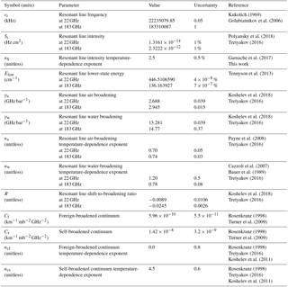
For the resonant absorption, the following parameters are relevant: line frequency (νi), intensity (Si) and its temperature coefficient (nS), the lower-state energy (Elow), air and water broadening (γa and γw) and their temperature-dependence exponents (na and nw), and the shift-to-broadening ratio (Ri). The uncertainty estimates for most of these parameters are given by Tretyakov (2016) within a review and expert assessment. The only exceptions are the uncertainty estimates for γa, γw, and Ri at 22 GHz taken from the more recent investigation of Koshelev et al. (2018) and the uncertainty for nS, which has been independently estimated within the 200–400 K temperature range as the maximal difference between numerical calculation of the partition sums at various temperatures published by Gamache et al. (2017) and their power approximation .
For the continuum absorption, four parameters are relevant, namely the self- and foreign-induced intensity coefficients and their respective temperature-dependence exponents (Cs,Cf, ncs, ncf). Uncertainties for Cs and Cf have been estimated considering that R17 adopts values adapted from Turner et al. (2009), who also provide an uncertainty estimate for the proposed multiplicative factors (0.79(18) and 1.11(10), respectively, for self and foreign coefficients). The uncertainties for ncs and ncf are estimated to overlap, within uncertainty, the values given by Koshelev et al. (2011) based on laboratory measurements. The resulting uncertainties (0.6 and 0.8, respectively) are more conservative than those provided originally (Liebe and Layton, 1987; Liebe et al., 1993).
The sensitivity analysis shows that among the 19 model parameters that were perturbed by the estimated uncertainty (Table 1), only 6 impact the modeled downwelling 20–60 GHz TB for more than 0.1 K: Cs, Cf, ncf and Si, γi,a, Ri at 22 GHz. The sensitivity of 20–60 GHz TB to perturbations to these six parameters is shown in Fig. 2. The impact of both positive and negative perturbations is shown; their symmetry with respect to the zero line suggests that estimated uncertainties represent small perturbations satisfying the linear assumption in Eq. (17). These six parameters are considered in Sect. 4 for an evaluation of their covariance. Although we note that Tretyakov (2016) indicates larger uncertainty for ncs at temperatures lower than 300 K, it was found that even considering 5 times larger uncertainty (to cover within uncertainty the value given for the range 270–300 K, i.e., 7.6(6)), the impact remains small for the relatively cold climatology. Thus ncs is not considered for the analysis in Sect. 4.
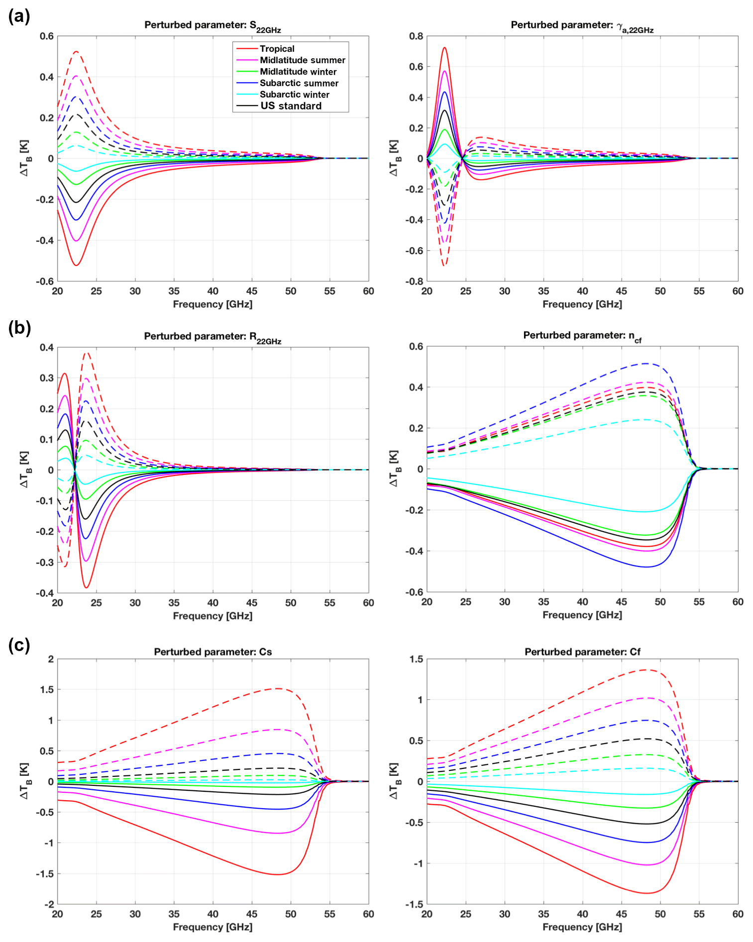
Figure 2Sensitivity of modeled TB to water vapor absorption parameters. (a) Line intensity (Si) and air broadening (γi,a) at 22 GHz. (b) Shift-to-broadening ratio (Ri) at 22 GHz and foreign-broadening temperature-dependence exponents (ncf). (c) Self-induced (Cs) and foreign-induced (Cf) broadening coefficients. Solid lines correspond to negative perturbation (value − uncertainty), while dashed lines correspond to positive perturbation (value + uncertainty).
3.2 Sensitivity to oxygen parameters
Oxygen absorption includes the zero-frequency band, fine structure spectrum, and pure rotational resonant transitions. The R17 model includes 49 oxygen absorption lines, of which 37 are within the 60 GHz band, 1 is at 118 GHz and the remaining 11 are in the millimeter to sub-millimeter range (200–900 GHz). Uncertainties for the oxygen parameters were either retrieved from the spectroscopic literature or, where not available, estimated from an independent analysis of measurement methods.
For the resonant absorption, the following parameters are relevant: line frequency (νi), intensity (Si) and its temperature-dependence exponent (nS), the lower-state energy (Elow), air broadening (γa) and its temperature-dependence exponent (na), normalized mixing coefficient (yi) and its temperature-dependence coefficient (Vi), and the water-to-air broadening ratio (rw2a).
The uncertainty estimates for most of these parameters are given by Tretyakov et al. (2005). In particular, Tretyakov et al. (2005) provide frequency uncertainty for 27 lines (N from 1 to 27, where N is the O2 rotational quantum number). For the other lines, the maximum uncertainty value has been assumed (i.e., 17 kHz), which is conservative with respect to HITRAN.
Resonant line intensities and lower-state energies are taken from the HITRAN 2004 database (Rothman et al., 2005). Although newer calculations are available in HITRAN 2016 (Gordon et al., 2017), the differences are within the assumed uncertainty at 1 % and 0.25 %, respectively. The latter is a rather conservative estimate, though its contribution turned out to be irrelevant. Note that the 1 % uncertainty in O2 line intensities is considered to originate mainly from the uncertainty of experimental measurements of electronic transition band-integrated intensities, which were used for intensity calculations of microwave lines. This uncertainty should be correlated for all lines by the principle of determination and thus we assume a single variable affecting all the lines. The uncertainty of the nS value for the 200–350 K temperature range was evaluated the same way as for water vapor lines, i.e., comparing partition sum calculations by Gamache et al. (2017) with their power-law approximation.
Values for oxygen line air-broadening and mixing parameters are taken from Tretyakov et al. (2005). Line-broadening parameters are measured through low-pressure laboratory experiments. Since individual lines are isolated at low pressures, no correlation is considered between parameters of different lines. Mixing parameters are determined at higher pressures, and their values are correlated with the previously determined low-pressure parameters. So, the line-mixing parameters are correlated with both themselves and the line air-broadening parameters. Because of this relationship, consistency requires that the number of considered line widths and the number of considered mixing coefficients should be the same. Tretyakov et al. (2005) derived mixing coefficients for lines with N from 1− to 33+ (34 in total), then extrapolated to lines with N > 33 (i.e., four weak lines of the 60 GHz complex). Thus, we first investigated the impact of these remaining four and the 11 rotational higher-frequency lines on 20–60 GHz TB by considering conservative and completely correlated uncertainty estimates (10 % for line-broadening and 20 % for line-mixing parameters). The impact was found to be negligible (< 0.1 K) and thus these 15 lines are not further considered in the following analysis. For the remaining 34 lines (N from 1− to 33+), the uncertainty for line air-broadening, mixing, and mixing temperature-dependence coefficients is evaluated through the full covariance matrices, so their treatment is postponed to Sect. 4.
For the air-broadening temperature-dependence coefficient, R17 retains a uniform value (0.8) for all lines (Liebe, 1989). We assume 0.05 uncertainty, which covers more recent measurements from Makarov et al. (2008) and Koshelev et al. (2016). Since R17 adopts the water-to-air broadening ratio rw2a, its value and uncertainty are respectively estimated as the mean and standard deviation calculated by Koshelev et al. (2015) from a set of 19 measurements (N from 1 to 19).
For the zero-frequency absorption, two parameters are relevant: the intensity () and broadening (γ0) of the pseudo-line. The intensity of the zero-frequency absorption is from the Jet Propulsion Laboratory (JPL) catalogue (https://spec.jpl.nasa.gov/, last access: 1 May 2018; Pickett et al., 1998). For the zero-frequency line broadening, consideration of the measurements cited in Danese and Partridge (1989), as well as those of Ho et al. (1972) and Kaufman (1967), lead us to assign an uncertainty of 50 MHz bar−1 to the absorption model's value of γ0=560 MHz bar−1 at 300 K. Note that uncertainties in the intensity and broadening coefficients of the zero-frequency component are negatively correlated because it is very difficult to measure the broadening independently of the intensity for this pseudo-line. This estimate based on the spread of published measurements accounts for the combination of intensity and broadening uncertainties.
The sensitivity analysis shows that among the model parameters in Table 2, which were perturbed by the estimated uncertainty, only the following impact the modeled downwelling 20–60 GHz TB for more than 0.1 K: Si, γa, na, yi, Vi, and γ0. The sensitivity of 20–60 GHz TB to perturbations to these parameters is shown in Fig. 3. As for water vapor, the impact of positive and negative perturbations is symmetric with respect to the zero line, suggesting that the linear assumption is valid for the estimated uncertainties. Note that the perturbation to Si and na affects all lines simultaneously, while the other resonant line parameters have been perturbed line by line. Although for the present ground-based application the uncertainty of only a few lines is relevant, we prefer to keep all 34 to make the calculation of the parameter uncertainties more generally useful (e.g., for satellite observations). Thus, the above six parameters (Si, γa, na, yi, Vi, γ0) are considered in Sect. 4 for an evaluation of their covariance. While for Si, na, and γ0 we consider three scalar parameters, for γa, yi, and Vi we consider 34 lines (N from 1− to 33+), leading to 34 coefficients for each parameter type.
Table 2List of oxygen parameters perturbed in the sensitivity analysis. * Tables 1 and 5 from Tretyakov et al. (2005).
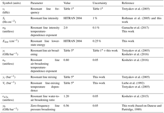
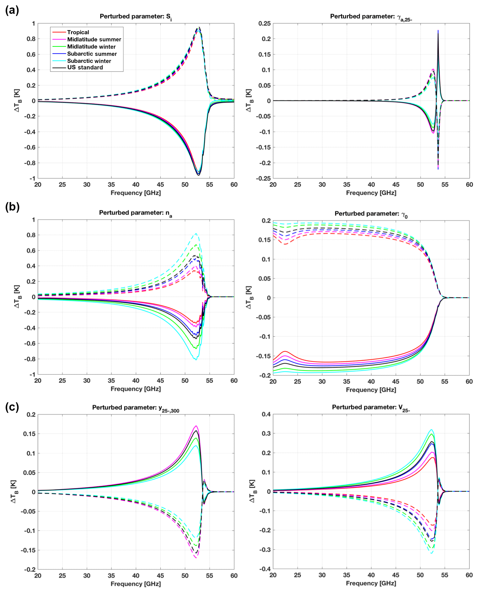
Figure 3Sensitivity of modeled TB to oxygen absorption parameters. (a) Line intensity (Si) and air broadening (γi,a). (b) Air-broadening temperature-dependence exponents (na) and nonresonant pseudo-line broadening (γnr). (c) Mixing coefficients (yi) and mixing temperature-dependence coefficients (Vi). Note that the perturbation to Si and na affect all lines, while for the other resonant line parameters we show the impact of the perturbation to just one line () as an example. Solid lines correspond to negative perturbation (value − uncertainty), while dashed lines correspond to positive perturbation (value + uncertainty).
The sensitivity analysis of Sect. 3 shows that the absorption model uncertainty on downwelling 20–60 GHz TB is dominated by the uncertainty on 6 spectroscopic parameters for water vapor and up to 105 parameters for oxygen. For these parameters, we require the full covariance matrix of parameter uncertainties to compute the uncertainty of calculated TB at any given frequency. This section summarizes the methods used to estimate the uncertainty covariance matrix, including the off-diagonal terms giving the covariance of each parameter with the others. Additional details can be found in Rosenkranz et al. (2018) (abbreviated as R18 below). However, the analysis here differs in three respects from the preliminary version in R18: the method of estimating Cov(Cf,Cs), the use of a smaller uncertainty for γ0, and the inclusion of Cov(γ0,na), which was neglected in R18.
Although we use different methods to estimate covariances depending on how the parameter values were measured, some general principles apply. If a set of variables ai has a causal dependence on another set of variables bk,
and the b values have an uncertainty covariance matrix Cov(b), then
where the angle brackets denote the expectation value, and the b values contribute an amount
to the uncertainty covariance of the a values. There may also be other contributions to Cov(a).
A probability distribution can be conditional, and the uncertainty of one parameter may be conditioned on an assumed value for a different parameter. Sometimes reported values of a parameter or set of parameters have been adjusted to fit measurements, while the experimenters considered other relevant spectroscopic parameters as fixed. Now if we wish to include in our analysis the uncertainty of one of the latter parameters (b) and it has a covariance with a fitted parameter a, the influence of b on a will increase the uncertainty of a above that which was found in the original experiment. That increment of variance is also given by Eq. (21), which in the scalar case is equivalent to
4.1 Uncertainty covariance matrix for water vapor parameters
Section 3.1 shows that for water vapor absorption six spectroscopic parameters dominate the uncertainty of modeled 20–60 GHz TB: three related to the continuum (Cs, Cf, ncf) and three to the 22 GHz resonant line (Si, γi,a, Ri). Sections 4.1.1–4.1.3 describe the methods used to estimate the covariances of these six water vapor spectroscopic parameters. Although the covariance matrix is the basic object needed for calculation, Table 3 lists both the estimated covariances of water vapor parameter uncertainties and the corresponding correlation coefficients because the latter are more easily comprehended, being pure numbers and normalized to the interval (). The numerical values of the full covariance matrix are also provided in the Supplement (in ASCII and NetCDF formats).
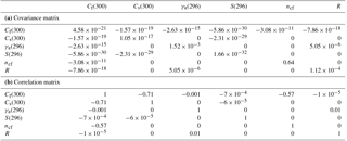
Table 3Covariance (a) and correlation (b) matrices corresponding to spectroscopic water vapor parameter uncertainties as derived in Sect. 4. Note that Cf and Cs are evaluated at T0=300 K, while γa and S are evaluated at T0= 296 K.
4.1.1 Covariance between water vapor line parameters
Intensity, width, and shift affect a line profile in different ways. But even if the original spectroscopic measurements covered the line profile adequately, a noticeable negative correlation between width and intensity arises if both are simultaneously estimated from measured absorption. In the present case, the only water line that survived the sensitivity screening for the 20–60 GHz band is the one at 22.2 GHz; the intensity used here was calculated independently from the width (Rothman et al., 2013), and the width was measured without using that intensity (Payne et al., 2008). Therefore, we consider errors in those two parameters to be uncorrelated. However, the absorption model code under investigation here (R17) uses the aforementioned ratio of shift to width (, where δa and γa are respectively the shift and width coefficients). As shown in R18, that introduces a covariance between R and γa of
where is the uncertainty variance of γa, and it corresponds to the small correlation of +1 % shown in Table 3 (positive because the nominal value of R is negative for this line).
4.1.2 Covariance between Cf, Cs, and other water vapor parameters
By definition, the water vapor continuum is the remainder after the contribution of local resonant lines has been subtracted. Thus, if a line width is revised, the continuum should also be revised to compensate for and reproduce as well as possible the original brightness temperature measurements of Turner et al. (2009) from which the continuum was derived. That was done by adjusting the continuum coefficients Cf and Cs for use with updated line parameters in R17. It should be the case no matter which line is revised. If we separate the model parameters into continuum (con) and line types, then as discussed in R18, the above statements are equivalent to requiring that for each line separately, the covariance between the continuum and line parameters and the line-parameter covariance matrix satisfy
In order for the above equation to hold over a range of humidity, it should apply to self and foreign gas effects separately. Both R and γa apply to dry air, so we set Cov( and Cov(Cs, . On the other hand, line intensity S affects both components of the continuum, with resulting covariances; then Eq. (24) can be solved for Cov(pcon, S) by making (see R18). As shown in Table 3b, the correlations of the continuum parameters with the 22 GHz line parameters are very small because this is one of the weaker water lines. If our matrix had included parameters for the 183 GHz water line, their covariances with the continuum might well be significant.
Although ncf, the continuum foreign-broadening temperature exponent, is not a line parameter, it was held fixed by Turner et al. (2009) in fitting Cf and Cs to the measured TB. Therefore, any subsequent change in ncf should require a compensating change in Cf; hence, from Eq. (24)
which turns out to produce a significant covariance (Table 3a). If Cf is thus compensated for, Cs should not change, so Cov(Cs, ncf) =0.
4.1.3 Covariance between Cf and Cs
For the water vapor continuum, R17 adopts the multipliers proposed by Turner et al. (2009) to the R98 parameter values of Cf and Cs, with small readjustments to accommodate the updated line widths in R17. Turner et al. (2009) derived the multipliers by adjusting them to fit ground-based radiometer measurements at 150 GHz. The simultaneous fitting of two coefficients results in a correlation between them.
When brightness temperature measurement errors are uncorrelated, with variance , a least-squares fit (see, e.g., van der Waerden, 1969; Stuart and Ord, 1991) results in the parameter-error covariance matrix
in which C is a vector containing the elements Cf and Cs and κ is a matrix with elements
where the subscript “m” is the index for the measurements of TB and indexes i and j equal 1 for Cf or 2 for Cs; the derivatives are to be evaluated for each atmospheric profile corresponding to TBm at the fitted values of Cf and Cs. When the correlation coefficient ρfs between Cf and Cs uncertainties is evaluated from Eq. (26), cancels, as does the determinant except for its sign, which in this case is positive. Thus, for the simple case of the 2×2 matrix,
Although Turner et al. (2009) do not give the correlation coefficient, it can be estimated from a simulation covering the same range of integrated water vapor content, 0.37 to 2.76 cm. We used 12 values of humidity distributed over this range in a subarctic summer model atmosphere, yielding , which is (presumably) approximately what Turner et al. would have calculated. Then using the experimentally determined uncertainties from Table 1, we have (which is ∼11 % larger than previously estimated in R18 by means of an analogy with data from Payne et al., 2011).
Turner et al. (2009) held other parameters constant while adjusting the continuum coefficients Cf and Cs. When we introduce a variance of ncf and its covariance with Cf (see Sect. 4.1.2), then as discussed in reference to Eq. (22), a corresponding increase by [Cov(Cf, ]2 to the experimentally determined variance of Cf is required. That increases from to , which is the value in Table 3a. However, when Cov(TB) is computed this increased variance will be offset by the negative contribution of Cov(Cf, ncf). (Had ncf been included in the least-squares fit, then it would have been a 3×3 matrix, which would have produced a different result originally.) Variance contributions from the 22 GHz line parameters are negligible. The correlation coefficients in Table 3b were then computed using the modified value of .
4.2 Uncertainty covariance matrix for oxygen parameters
The sensitivity analysis in Sect. 3.2 shows that for oxygen absorption six spectroscopic parameter types dominate the uncertainty of modeled 20–60 GHz TB: line intensity (Si), air broadening (γa) and its temperature-dependence exponent (na), normalized mixing coefficient (yi) and its temperature coefficient (Vi), and zero-frequency broadening (γ0). Parameters na and γ0 are scalar, while γa, yi, and Vi are vectors of 34 components (for lines with N from 1− to 33+); although Si is also a vector, its percent of uncertainty is a scalar, thus leading to a 105×105 uncertainty covariance matrix. Sections 4.2.1–4.2.4 describe the method used to estimate the uncertainty covariance of these 105 oxygen spectroscopic parameters with respect to each other. The numerical values of the full covariance matrix are provided in the Supplement (both in ASCII and NetCDF formats). Figure 4 depicts the resulting matrix as a color-scale image of sign-adjusted correlation coefficients. For any two parameters p1 and p2 with nominal values and and correlation coefficient ρ(p1,p2), the sign-adjusted correlation is defined as
If and have the same sign, ρSA(p1,p2) reduces to ρ(p1,p2). If the signs differ, then ρSA(p1,p2) has sign opposite to ρ(p1,p2). If the standard deviations are small compared to the nominal values, as is generally the case here, ρSA(p1,p2) gives the correlation between the absolute values of the parameters. ρSA(p1,p2) can be negative, as is the case for the relation between line intensities and the mixing coefficients, which indicates that a positive error in intensities results in underestimation of line mixing.
4.2.1 Covariance between oxygen line-broadening coefficients
Values for oxygen line air broadening are taken from Tretyakov et al. (2005). They measured N2 broadening of O2 lines with rotational quantum numbers N from 1 to 19 and self-broadening for N from 1 to 27 (the 1− line had previously been measured in Tretyakov et al., 2004). Uncertainties of the measured line widths were estimated here by considering the results of Tretyakov et al. (2005) and Koshelev et al. (2016) together. Three sources were assumed to contribute to the error budget: (i) the statistical uncertainty was determined from a Padé approximation (Koshelev et al., 2016) of the N dependence of γa, weighting all data by their respective 1∕σ; (ii) a pressure gauge uncertainty of 0.25 %; and (iii) an uncertainty of 0.5 ∘C for the temperature sensors. The total uncertainty for each line's air broadening was determined as the root sum of squares. Uncertainties calculated for all lines with N≤19 are close to each other at ∼0.014 GHz bar−1, so we use this value for all lines with N≤19. Even though the lines were measured separately by Tretyakov et al. (2005), the pressure sensor and temperature sensor uncertainties contain systematic components that (due to the same experimental setup) may have introduced minor correlations between line widths. However, the broadening parameter uncertainty originates mainly from the unknown baseline of the apparatus. The work by Koshelev et al. (2016), in which different sensors were used, confirmed that there was no noticeable bias in the earlier measurements. This reasoning allows us to neglect potential correlations of the measured line widths.
For the remaining lines, Tretyakov et al. (2005) extrapolated the broadening coefficients by a straight-line graphical method, assuming a pivot value (hereafter indicated with subscript *) such that
where for N2 broadening and 17 for pure O2; μ is the slope of the straight line and γ* averages the N− and N+ lines for N*. The extrapolation introduces correlations among those coefficients and between them and the measurements with N > N*, which were used to determine the straight line, as discussed in detail in R18. Also, the uncertainties of the extrapolated broadening coefficients increase with N up to a maximum of 0.032 GHz bar−1 at N=33. For the purpose of estimating covariances, the extrapolation was modeled as though it was a formal linear regression. This assumes that a straight line is the right extrapolation method, which seems reasonable, although it cannot be tested because the very weak lines have not been measured.
Figure 4 represents the sign-adjusted correlation coefficients as a color image. The extrapolated coefficients (nos. 24–37 in Fig. 4) are strongly correlated among themselves, although not perfectly. On the other hand, the uncertainty of the zero-frequency broadening coefficient (no. 3) is assumed to be uncorrelated with the line air-broadening uncertainties. Figure 5 shows the γa values given by Tretyakov et al. (2005) and the associated uncertainties as estimated above, together with the values and the uncertainties of y and V, which are treated in the next two sections.

Figure 4Uncertainty matrix for oxygen absorption as a color-scale image of sign-adjusted correlation coefficients (ρSA). See Eq. (29) in Sect. 4.2 for the definition of ρSA. The y axis label shows selected parameter indexes. The parameters are ordered as follows: no. 1) S(300), no. 2) na, no. 3) γ0(300), nos. 4–37) γa(300), nos. 38–71) y(300), nos. 72–105) V. The last three parameter types are ordered following the O2 rotational quantum number , 1+, 3−, … 33−, 33+.
4.2.2 Covariance between oxygen line-mixing coefficients
Values for oxygen line-mixing coefficients are taken from Tretyakov et al. (2005), in which mixing coefficients were determined from measurements made near 1 atm of pressure and temperatures near 22–24 ∘C by an algorithm that makes them dependent on the other parameters. Hence, uncertainties in those other parameters contribute uncertainties to the mixing coefficients as well as correlations with them. R18 shows that the estimation algorithm can be represented in the form of a vector equation:
where y is the vector of normalized mixing coefficients defined by Eq. (13), A is the matrix representing the linear estimation operation, α is the vector of absorption measurements, and αb is a vector of absorption calculated from a baseline mixing coefficient set b. Hence, applying Eqs. (20–21),
where I is the identity matrix, Ky and Kγ are matrices of partial derivatives of baseline absorption with respect to y and γ, respectively, and σS is the fractional uncertainty in line intensities. The first term above is the contribution of measurement noise with variance and the third and fourth terms represent the uncertainty contributed by line widths and intensities in the derivation of the y values. In Tretyakov et al. (2005), the baseline mixing coefficients were taken from Liebe et al. (1992), who derived them by essentially the same algorithm with very similar smoothing characteristics. Therefore, in the second term of Eq. (32), the projection operator (I – A Ky) should remove the variation of the mixing coefficients obtained in Liebe et al. (1992), and the only part that will survive is the original baseline, which is attributable to the coupling between the positive-frequency resonances and the negative-frequency and zero-frequency bands. In R18, the contribution of the second term in Eq. (32) is estimated as to each element of Cov(y), with νb= 40 GHz.
The mixing coefficient of the 1− line was measured separately in Tretyakov et al. (2004), so it is not correlated with the others. Their estimated uncertainty for its value is bar−1. The y values measured at 295 K in Tretyakov et al. (2005) were adjusted to 300 K using the temperature coefficients given by Liebe et al. (1992). However, for the sake of simplicity that small correction was ignored here, and the uncertainties of mixing coefficients at T0=300 K are considered to be the same as the measured coefficients. Hence, we assume no correlation between the line-mixing coefficients at 300 K and the line-mixing temperature coefficients, since they originate from different laboratories.
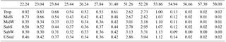
Table 4Uncertainty on simulated TB (σ(TB)) at 14 HATPRO channel central frequencies due to the uncertainty in O2 and H2O absorption model parameters. σ(TB) is computed as the square root of the diagonal terms of Cov(TB), which was estimated considering the six climatological atmospheric conditions introduced in Fig. 1.
4.2.3 Covariance between oxygen line-mixing temperature coefficients
The first-order line-mixing parameterization in R17 is given by Eq. (13). Table 5 of Tretyakov et al. (2005) lists coefficients a5 and a6 for each line, a notation retained from Liebe et al. (1992). These are related to the line-mixing coefficients as and temperature coefficients as Vi=a6. Liebe et al. (1992) measured line mixing at three temperatures and determined a6 by a linear regression versus θ. We calculate the covariance matrix for the V values as
where xk is the influence given by the regression to the mixing coefficients at Tk in determining the V values (see R18). The baseline b does not contribute to V because the three values of xk sum to zero. The first term in Eq. (33) is the measurement noise contribution. Unlike the model parameters that are defined at 300 K, the V coefficients depend on the value of na, and its uncertainty contributes the second term in Eq. (33); the derivatives were evaluated by finite differences. The third term in Eq. (33) results from a comparison of Liebe et al. (1992) to later work, which indicates that it contained some systematic errors in intensities (generally ∼1 % or less) and in line widths (typically ∼3.3 % smaller than those measured in Tretyakov et al., 2005). The effect on V of those systematic errors, , was also evaluated numerically, as described in R18. We combine systematic and random errors in Eq. (33), as suggested by JCGM (2008).
4.2.4 Covariance between different oxygen parameter types
The discussion in connection with Eqs. (20) and (21) indicates that corresponding to the second, third, and fourth terms in Eq. (32) for Cov(y), there must be uncertainty covariances between the line-mixing coefficients of the 60 GHz band and the line width and intensity parameters.
The negative signs in these equations originate because the computed baseline absorption occurs with a minus sign in the determination of the y coefficients. Likewise, corresponding to the second term of Eq. (33) for Cov(V), there is an uncertainty covariance between each V coefficient and na:
The value of γ0 was determined by Danese and Partridge (1989) from radiometer measurements of the sky at a mountain site. Because the atmospheric emission depends on the temperature profile, a covariance with na results. We calculate a typical value for that site (White Mountain) of GHz bar−1; thus, in analogy with Eq. (25),
corresponding to . The increment of uncertainty variance for γ0 due to Eq. (38) is 2 orders of magnitude smaller than the value assigned to and therefore negligible.
The uncertainty covariance matrices estimated in Sect. 4 for water vapor and oxygen spectroscopic parameters are combined together to form Cov(p), a 111×111 matrix. The two matrices are combined block-diagonally, i.e., assuming no cross-covariances between H2O and O2 absorption model parameter uncertainties. Thus, Cov(p) represents the uncertainty covariance matrix of the H2O and O2 absorption model parameters that were judged relevant for downwelling TB in the 20–60 GHz range. In this section, Cov(p) is propagated to estimate its impact on simulated downwelling TB and ground-based temperature and humidity retrievals.
5.1 Uncertainty on simulated brightness temperatures
The propagation of the absorption model parameter uncertainty to calculated TB is given by Eq. (18), which requires knowledge of Kp, i.e., the Jacobian of calculated TB with respect to model parameters. The Jacobian Kp is a nfreq×npar matrix, where nfreq is the number of frequency for which the TB uncertainty should be calculated and npar is the number of considered parameters, 111 in our case. Here we set nfreq=437, which includes 401 equally spaced frequencies from 20 to 60 GHz (by 0.1 GHz increment), plus 36 corresponding to the central frequencies of two widely deployed commercial MWRs, i.e., the HATPRO (Rose et al., 2005) and MP-3000A (Ware et al., 2003). The Jacobian Kp has been estimated numerically by perturbing each parameter individually by a small amount (corresponding to the parameter 1σ uncertainty). To represent different climatology conditions, six realizations of Kp have been computed using the six atmospheric climatology conditions introduced in Fig. 1. Thus, Cov(TB) is computed from Eq. (18) using Cov(p) and Kp estimated as above. Figure 6 reports σ(TB), which is the square root of the diagonal terms of Cov(TB), for the whole 20–60 GHz range and for the six atmospheric climatology conditions. Similarly, σ(TB) values at the central frequencies of the two commercial MWRs are reported in Table 4 (HATPRO, 14 channels) and Table 5 (MP-3000A, 22 channels).
Table 5As in Table 4 but at 22 central frequencies of MP3000-A channels.
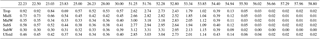
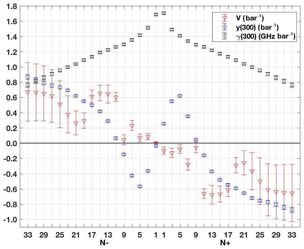
Figure 5Oxygen line parameters as a function of rotational quantum number N: line width γa(300) (squares), line mixing y(300) (circles), and line-mixing temperature coefficients V (triangles). Error bars indicate ±1σ uncertainties.
To appreciate the dominant contributions within the frequency range, the different parameters have been grouped into seven types: intensity S (for both O2 and H2O), O2 line width γa, O2 zero-frequency line width γ0, O2 line mixing (y), O2 line-mixing temperature dependence (V), H2O continuum, H2O line width γa, and shift-to-width ratio R. The contribution of each type to TB uncertainty was estimated by propagating the uncertainty covariance matrix reduced to the size of the parameters belonging to that type only. Figure 7 shows the resulting contributions computed for the tropical climatology conditions. We choose tropical conditions so that features at 22.2 GHz are evident above the continuum absorption.
Thus, looking at Figs. 6–7 and Tables 4–5, it seems convenient to discuss the 20–60 GHz range in four parts: the proximity of the 22.2 GHz water vapor line (20–26 GHz), the atmospheric window (26–45 GHz), the low-frequency oxygen wing (45–54 GHz), and the opaque oxygen band (54–60 GHz). In the following, the contribution dominance is inferred from Fig. 7, while the typical values are inferred from Fig. 6 and Tables 4–5.
-
20–26 GHz: TB uncertainty is dominated by uncertainty in water vapor line width and shift coefficients, going from ∼0.3 K (subarctic winter) to nearly 1.0 K (tropical).
-
26–45 GHz: TB uncertainty is dominated by uncertainty in water vapor continuum parameters, increasing with frequency from ∼0.4 to 1.2 K, with ∼0.2 K larger uncertainty in tropical with respect to other climatology conditions.
-
45–54 GHz: TB uncertainty is dominated by uncertainty in oxygen line-mixing parameters (up to 2 K). Water vapor continuum, line-mixing temperature dependence, and line intensity parameters also contribute to a lesser extent (up to 1.0–1.2 K) at a respectively increasing frequency. The total TB uncertainty decreases with increasing temperature, which is lower for tropical (up to 2.7 K) than for subarctic winter (up to 3.4 K) conditions.
-
54–60 GHz: TB uncertainty is below 0.5 K at 54–55 GHz and rapidly approaches zero for frequencies above 55 GHz. In this very opaque region, the contribution of absorption model parameters to simulated ground-based TB is negligible.
The qualitative conclusions above may sound somewhat obvious, at least to microwave remote sensing experts. But the quantitative estimates are unprecedented to our knowledge, especially in light of the evaluation of the full uncertainty covariance matrix. One may wonder how high the contribution of covariance matrix off-diagonal terms is. To evaluate it, TB uncertainty has also been computed considering Cov(p) as a diagonal matrix (i.e., all uncorrelated parameters). The difference of σ(TB) computed considering the full uncertainty covariance matrix and a diagonal matrix is shown in Fig. 8. The contribution of off-diagonal terms goes from −1.2 to 0.6 K. It mostly affects the low-frequency oxygen wing, presumably due to line-mixing parameters and their temperature dependence, with sharp gradients in the 46–52 and 52–54 GHz frequency ranges. It also affects the atmospheric window, presumably due to water vapor continuum parameters, with a contribution of the order of −0.3 to −1.0 K. This demonstrates that off-diagonal terms cannot be neglected, especially in the uncertainty characterization of the window and low-opacity channels of the HATPRO and MP3000-A instruments.
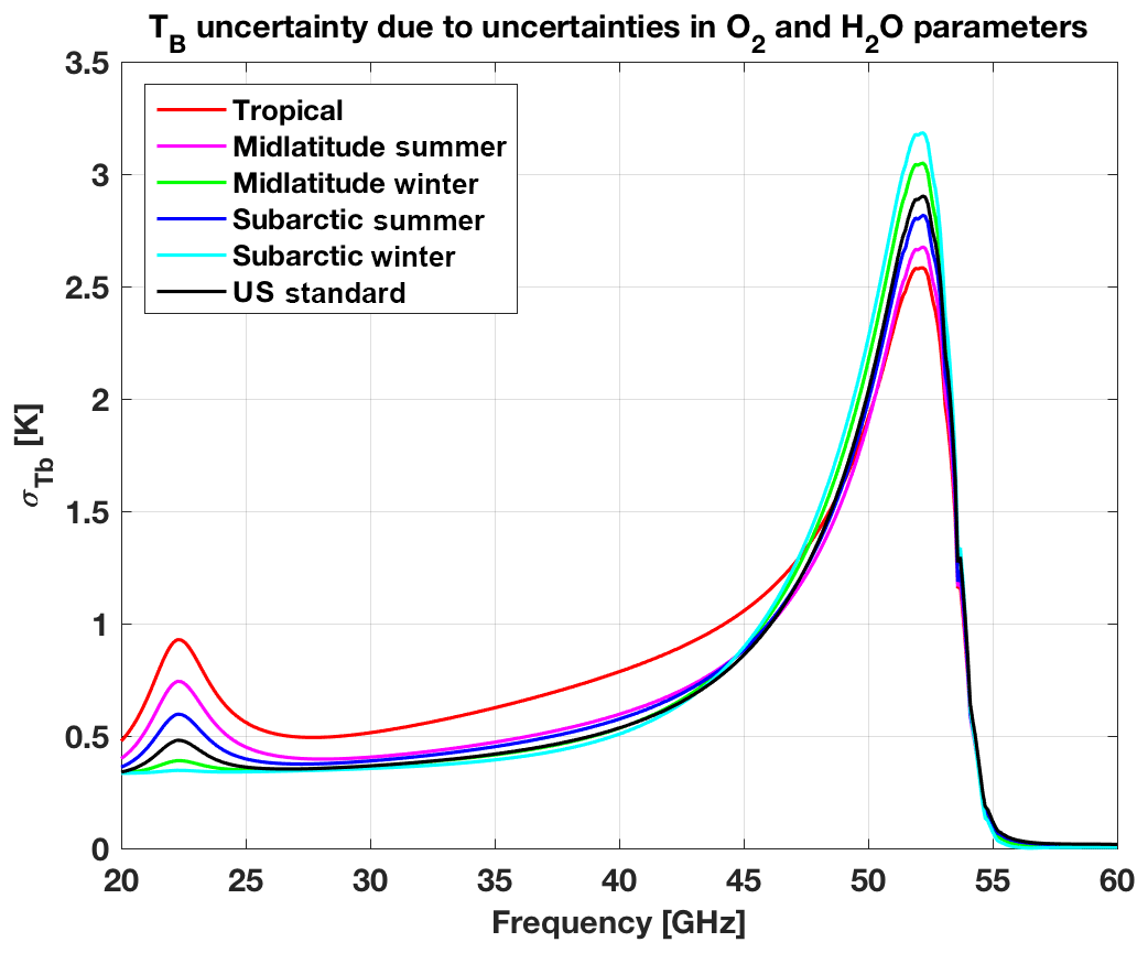
Figure 6Zenith downwelling TB uncertainty (σ(TB)) due to the uncertainty in O2 and H2O absorption model parameters. Six climatological atmospheric conditions (color coded) have been used to compute Kp. σ(TB) is computed as the square root of the diagonal terms of Cov(TB).
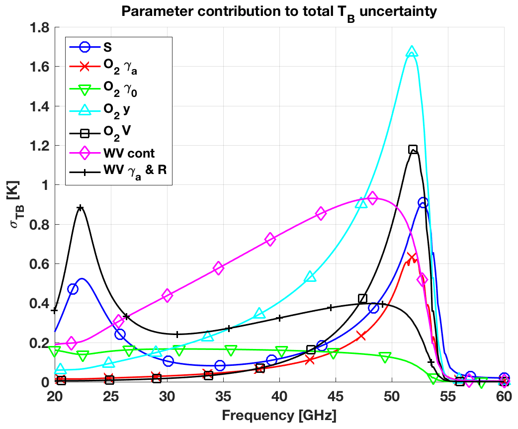
Figure 7Contributions to zenith downwelling TB uncertainty (σ(TB)) due to the different types of O2 and H2O absorption model parameters. Tropical climatology conditions are used here. The parameters are grouped into seven types: intensity S (for both O2 and H2O), O2 line width γa, O2 zero-frequency line width γ0, O2 line mixing (y), O2 line-mixing temperature dependence (V), H2O continuum, H2O line width γa, and shift-to-width ratio R.
Finally, it shall be noted that the output of this analysis is Cov(TB), i.e., the full covariance matrix of TB uncertainties. A graphical representation of Cov(TB) is given in Fig. 9 for HATPRO channels and US standard climatology. The resulting matrices computed for HATPRO and MP3000-A channels and the six considered climatology are provided in the Supplement.
Previous studies also reported values for σ(TB) (Hewison et al., 2006; Hewison, 2007) and Cov(TB) (Hewison 2006b), though these were estimated from relative TB differences computed with a set of absorption models available at that time. With respect to these values, we report (i) smaller uncertainty at 20–30 GHz channels due to improved accuracy of the 22 GHz line spectroscopic parameters and (ii) much larger uncertainty at 50–54 GHz channels due to the consideration of line-mixing parameter uncertainties, which likely canceled out partially in the relative TB difference approach used by Hewison (2006b, 2007).
5.2 Uncertainty on temperature and humidity retrievals
The uncertainty in absorption model parameters impacts the accuracy of geophysical variables retrieved from radiometric observations through inversion methods based on a forward operator. Here, the forward operator is a radiative transfer model (RTM) relying on the spectroscopic parameters to compute atmospheric absorption and emission and thus the measurable TB, from atmospheric thermodynamical profiles. Examples of such inversion methods are described in Cimini et al. (2006) and include simulation-based regression, artificial neural networks, and the optimal estimation method (OEM). The OEM is particularly suitable to investigate the uncertainty contribution of spectroscopic parameters, as it allows one to perform an assessment of the total statistical uncertainty, as well as of the forward model parameter uncertainty (Rodgers, 2000). For example, it has been used for a spectroscopic parameter sensitivity study for a millimeter to sub-millimeter limb sounder instrument (Verdes et al., 2005) and to estimate the impact of forward model parameters on the temperature retrieval from a multiple-channel Rayleigh-scatter lidar (Sica and Haefele, 2015).
Thus, let us consider the OEM formalism. Following Rodgers (2000), the total uncertainty covariance matrix of the retrieved atmospheric profile is
where Covm and Covs are respectively the measurement and smoothing uncertainty covariance matrices, while Covp is the model parameter uncertainty covariance matrix. Covp is related to Cov(p) through Kp, the Jacobian of the forward model with respect to the parameters p, and the sensitivity of the inverse method to the measurements (also called the contribution function or gain matrix) as
Assuming a linear Gaussian case as usual for ground-based radiometric retrievals of atmospheric temperature and humidity profiles (Löhnert et al., 2004; Cimini et al., 2006, 2010; Hewison, 2007) and calling Cov(ϵ) and Cov(xa) the covariance matrices of measurement and a priori background uncertainty, the gain matrix is given by (Rodgers, 2000)
where Kx is the Jacobian of the forward model with respect to the atmospheric state x. Finally, considering TB as the measurements and recalling Eq. (18), the model parameter uncertainty covariance matrix in Eq. (40) becomes
which contributes to the total profiling uncertainty as in Eq. (39). Note that Cov(TB) is the full spectroscopic parameter uncertainty covariance matrix estimated in Sect. 5.1. Accordingly, the combined uncertainty due to the O2 and H2O absorption model parameter is thus propagated into the retrieval space.
As an example of the spectroscopic contribution to profiling uncertainty we apply the approach described above to HATPRO channels (as in Table 4), specifically (i) seven K-band channels (22.24 to 31.40 GHz) and (ii) seven V-band channels (51.26 to 58.0 GHz), to compute the impact on specific humidity and temperature profile retrievals, respectively. For the sake of result reproducibility, simple diagonal Cov(ϵ) and Cov(xa) matrices are assumed here, with reasonable values resembling typical matrices adopted in ground-based microwave profiling (Martinet et al., 2015; Martinet et al., 2017). Specifically, we assume a constant uncertainty for TB measurements (, with K) and a priori temperature profile (, σT=1.5 K), while also assuming a decreasing-with-height uncertainty for a priori specific humidity profile (where z is height in kilometers, σQ(0)=3.2 g kg−1, and H=4 km). The a priori background xa and Jacobian Kx are defined on 101 pressure levels, from 0.005 to 1050 hPa. These levels are selected to be denser close to the surface (34 levels below 2 km), specifically for downwelling radiative transfer calculations. The vertical spacing of the adopted levels is given in De Angelis et al. (2016).

Figure 8Difference between σ(TB) as computed considering the full uncertainty covariance matrix and its diagonal matrix (i.e., off-diagonal terms are set to zero).
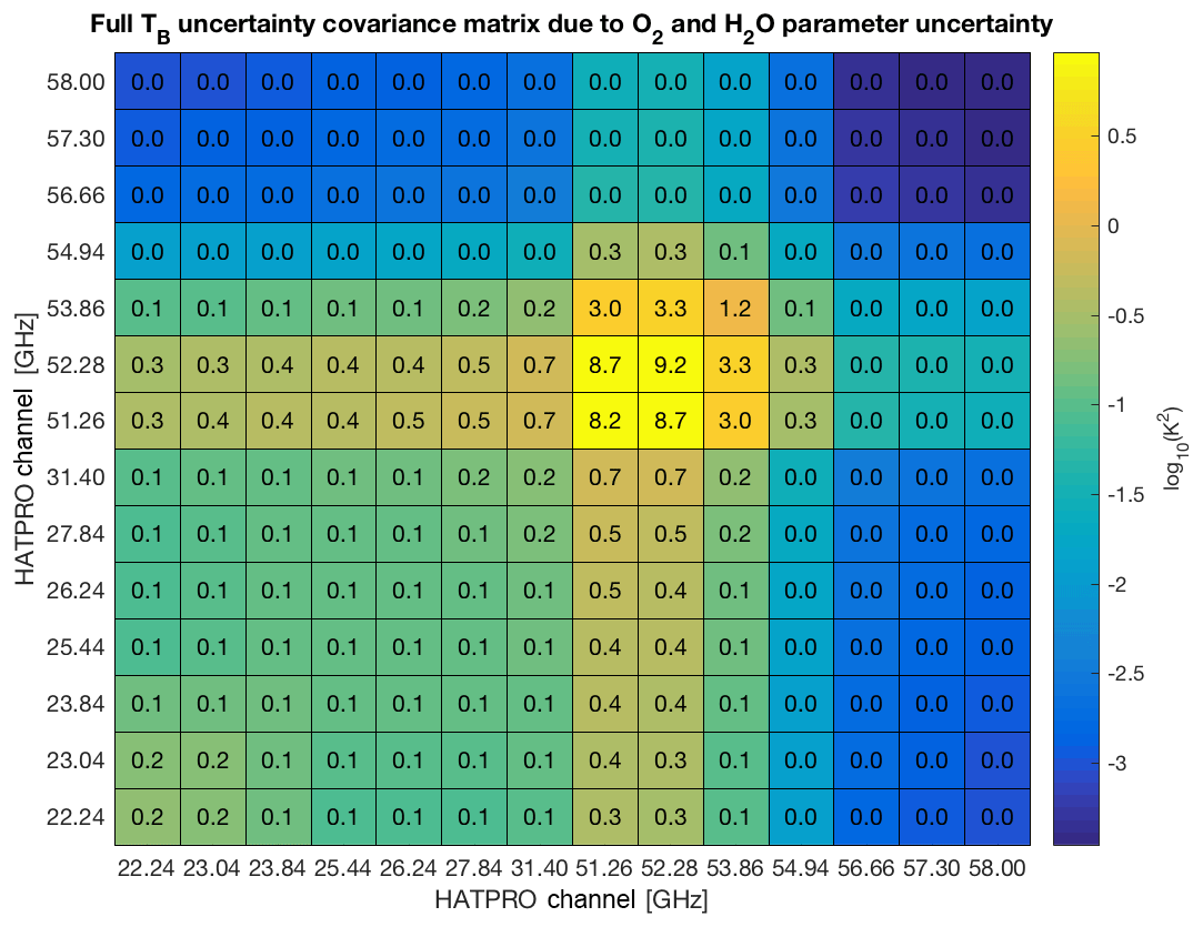
Figure 9TB uncertainty covariance matrix due to O2 and H2O absorption model parameter uncertainty at HATPRO channels for US standard climatology. Numbers in the table are in K2, while the color scale is in log10(K2).
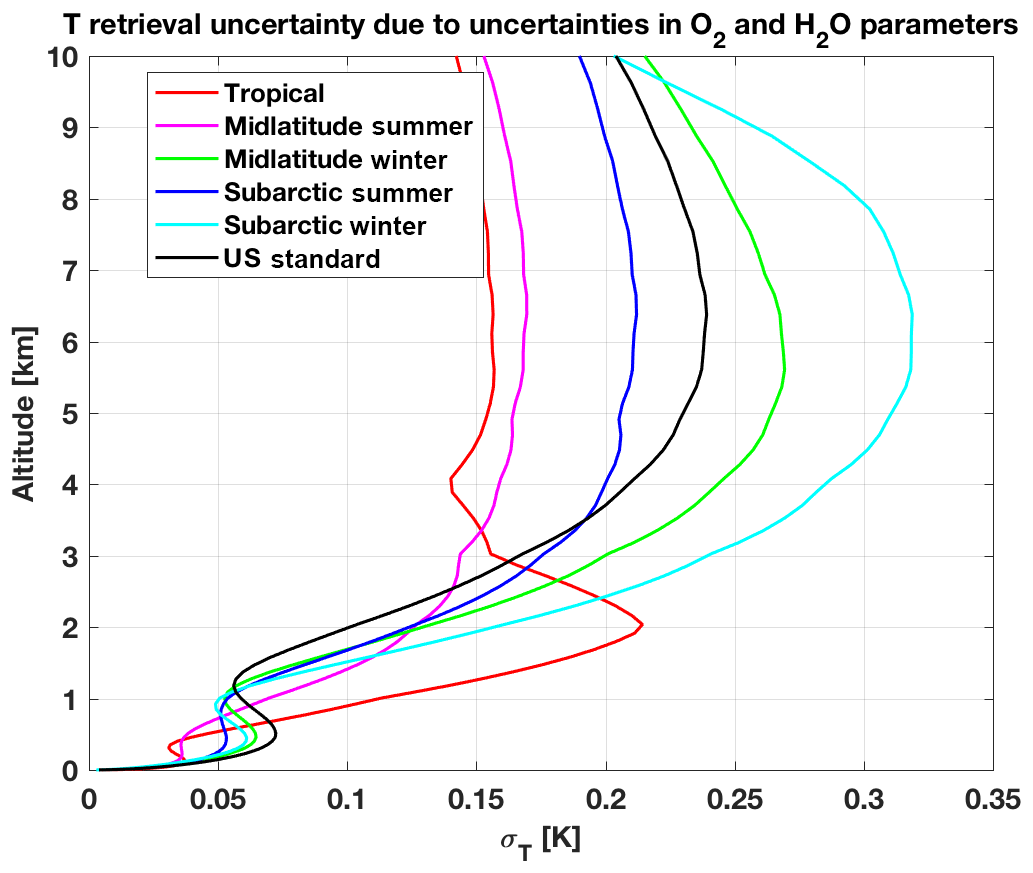
Figure 10Uncertainty in temperature retrievals from ground-based MWR due to the uncertainty in O2 and H2O absorption model parameters. The observation vector considered here consists of TB at the 14 HATPRO channels. Six climatological atmospheric conditions (color coded) have been used to compute Kb and Kx. The square roots of the diagonal terms of Covp are shown. 101 pressure levels from 0.005 to 1050 hPa are used here. These levels have been selected specifically to be denser close to the surface (34 levels below 2 km). The vertical spacing of levels is given in Fig. 1 of De Angelis et al. (2016).
The square roots of Covp diagonal terms are shown in Figs. 10 and 11 for temperature and specific humidity profiling, respectively. Note that these uncertainty profiles shall be considered just as relative, as they depend upon the vertical grid spacing and the choice of Cov(ϵ) and Cov(xa). Nonetheless, Figs. 10 and 11 show that the contribution of absorption model uncertainty to the profile retrieval uncertainty is generally not negligible. For temperature, the absorption model contributes less near the surface and more in the upper atmosphere; these are respectively the direct consequences of negligible uncertainty for O2 opaque channels (55–58 GHz) and significant uncertainty for O2 transparent channels (50–55 GHz). Above 3 km, the impact increases for colder and drier conditions. Though less clearly, this also holds below 3 km for all but tropical conditions, which show a peak around 2 km. This is due to the fact that lower V-band channels (51–52 GHz) gain sensitivity to boundary layer temperature as moisture increases. These channels are the most affected by absorption model uncertainty (Fig. 6 and Table 4) and thus contribute to larger temperature uncertainty in the lower layers. For specific humidity, the absorption model contribution to uncertainty simply increases with increasing moisture. This is a direct consequence of increasing K-band TB uncertainty corresponding to increasing moisture, as seen in Fig. 6. Values are particularly high for relatively drier climatology (e.g., arctic); this is simply a consequence of the assumed a priori σQ, which is typical of midlatitude climatology. Reducing σQ by a factor of 10 (to be closer to values for dry climatology), the uncertainty profile would be reduced roughly by the same factor.
With respect to the absorption model parameter contribution in Figs. 10 and 11, the uncertainty due to measurement noise (i.e., the diagonal terms of Covm) is of comparable magnitude, though with different vertical shape and little dependence on climatology (not shown). Note that in the actual retrieval process, the contribution of absorption model parameter uncertainty to the total profiling uncertainty can be equivalently treated as Covp or as adding an absorption model term to the measurement uncertainty, i.e., (Rodgers, 2000).
Radiative transfer models have general implications for atmospheric sciences, including meteorology and climate studies. Atmospheric absorption modeling is a key component of radiative transfer codes, which are extensively used for the retrieval of atmospheric variables and the assimilation of radiometric observations into NWP. Uncertainties in atmospheric absorption models thus contribute to the uncertainty of atmospheric retrievals and observations vs. background comparison. The analysis above shows a viable approach to quantify the uncertainties of atmospheric absorption modeling and the impact on radiative transfer calculations and atmospheric retrievals. The approach relies on the estimation of the full covariance matrix of parameter uncertainties, which is necessary to compute the uncertainty of calculated TB at any given frequency. The approach is general and not limited to any particular instrument, technique, or frequency range. The approach can be applied to any absorption model and it can be easily extended to other frequencies and observation geometry (e.g., from satellite). To demonstrate its use quantitatively, we apply this approach to a widely used microwave absorption model (R17, Rosenkranz 2017), focusing on the 20–60 GHz frequency range commonly exploited for atmospheric remote sounding by ground-based MWR profilers.
We have summarized the modifications made in the last 20 years to a reference absorption model (Rosenkranz, 1998), leading to the current version of the model R17. We reviewed the spectroscopic literature searching for uncertainty estimates affecting the spectroscopic parameters entering the absorption model code. In the considered frequency range, atmospheric absorption is dominated by water vapor and oxygen. The associated parameters and their uncertainties are reported in Tables 1 and 2, respectively, for water vapor and oxygen absorption. We performed a sensitivity analysis by perturbing each parameter by its estimated uncertainty and quantifying the impact on simulated TB for six climatology conditions. The uncertainty of the following parameters is found to impact 20–60 GHz TB calculations by more than 0.1 K in any of the considered climatologies. Concerning water vapor absorption, these are self- and foreign-continuum absorption coefficients, line broadening by dry air, line intensity, the temperature-dependence exponent for foreign-continuum absorption, and the line shift-to-broadening ratio. Concerning oxygen absorption, the dominating parameters are line intensity, line broadening by dry air, line mixing, the temperature-dependence exponent for broadening, zero-frequency line broadening in air, and the temperature-dependence coefficient for line mixing. Thus, from the initial set of 319 considered parameters, 111 are retained for further analysis (6 for water vapor and 105 for oxygen). For the retained parameters, we estimated the full uncertainty covariance matrix, i.e., including parameter uncertainty variances and cross-covariance between uncertainties of different parameters. Since the spectroscopic literature provides at most the uncertainties of individual parameters, but not the covariance between them, the off-diagonal terms of the uncertainty covariance matrix had to be estimated by investigating the possible correlation between the methods used to retrieve the parameter values. The full uncertainty covariance matrix (111×111) as estimated is provided in the Supplement.
Then, the contribution of the spectroscopic parameter uncertainties, including the covariance between them, to the uncertainty of simulated downwelling 20–60 GHz TB is calculated for six climatology conditions using the estimated uncertainty covariance matrix (Fig. 6). Dividing the 20–60 GHz range into four parts, typical TB uncertainties are (i) ∼0.3 K (subarctic winter) to nearly 1.0 K (tropical) at 20–26 GHz, (ii) ∼0.4 to 1.2 K with additional ∼0.2 K uncertainty in tropical conditions at 26–45 GHz, (iii) up to 3.4 K inversely proportional to temperature at 45–54 GHz, and finally (iv) below 0.5 K at 54–55 GHz rapidly approaching zero for frequencies above 55 GHz. The dominant uncertainty contributions are water vapor line width and shift at 20–26 GHz, water vapor continuum at 26–45 GHz, and oxygen line mixing at 45–55 GHz; finally, absorption model uncertainty becomes negligible at 55–60 GHz. Despite the fact that these qualitative conclusions may sound obvious, at least to microwave remote sensing experts, the quantitative estimates are unprecedented to our knowledge, especially in light of the evaluation of the full uncertainty covariance matrix. It is shown that off-diagonal terms affect the low-frequency oxygen wing, presumably due to covariance of line-mixing parameters and their temperature dependence, but also the atmospheric window, presumably due to covariance of water vapor continuum parameters. The total contribution depends upon frequency and ranges from −1.2 to 0.6 K, demonstrating that off-diagonal terms cannot be neglected, especially in the uncertainty characterization of window and low-opacity channels.
The resulting uncertainty on simulated TB is also calculated at the channels of two of the most common commercial MWRs, i.e., HATPRO and MP3000-A. The computed Cov(TB) values, of which one example is shown in Fig. 9, are provided for the two instruments and for the six climatology conditions in the Supplement. These matrices may be directly exploited as the additional observation uncertainty related to absorption model in any retrieval and data assimilation procedure exploiting either of the two instruments. Just to give an example, the absorption model uncertainty is propagated to ground-based MWR retrievals, showing its impact on retrieved temperature and humidity profiles for the six climatology conditions (Figs. 10 and 11). It is shown that the contribution of absorption model uncertainty to the profile retrieval uncertainty depends on climatology (increasing temperature uncertainty with decreasing average temperature, increasing humidity uncertainty with increasing moisture), and it is generally not negligible, though the actual values depend on retrieval settings (such as a priori information and vertical spacing, among others).
Finally, let us underline the fact that the presented uncertainty quantification contributes to a better understanding of the total uncertainty affecting radiometric products, thus reducing the chances of systematic errors in NWP data assimilation and observation-derived climate trends. Note that the presented uncertainty covariances of spectroscopic parameters are generally valid, while the TB sensitivity analysis and uncertainty quantifications are strictly valid only for the ground-based geometry and the considered frequency range. Future work may include the application of the proposed approach to higher frequencies and upwelling TB, requiring a new sensitivity analysis. Further modification to the R17 absorption model may be considered to account for recent findings from spectroscopic laboratory experiments (e.g., inter-branch coupling suggested by Makarov et al., 2013, temperature exponent na suggested by Koshelev et al., 2016, consideration of the speed dependence of the collisional relaxation effect influencing diagnostic line profiles as shown in Koshelev et al., 2018). In addition to uncertainties of parameters within a given absorption model, other errors can be contributed by approximations made in formulating the model, such as the H2O continuum formulation or neglect of higher-order line mixing in O2. Those uncertainties would need to be treated by a different analysis.

Uncertainty covariance matrices for the spectroscopic parameters considered here, as well as the resulting TB uncertainty covariance matrices for HATPRO and MP3000A channels, are available as a Supplement to this paper. The absorption model by Rosenkranz (2017) is available as a FORTRAN 77 code at https://doi.org/10.21982/M81013 (Rosenkranz, 2017). Older versions, including the one used here (15 May 2017), are available at http://cetemps.aquila.infn.it/mwrnet/lblmrt_ns.html (last access: 23 October 2018).
The following two sections review the set of modifications to the R98 model for water vapor and oxygen absorption, respectively, proposed in the open literature in the last 20 years and subsequently imported in the current R17 version of the model.
A1 Water vapor
The R98 model uses 15 water vapor lines, similar to the strongest lines used in MPM89, while the other 15 lines have been omitted as they were judged to have a negligible impact. For the water vapor continuum absorption, the model combines the foreign-broadened component from MPM87 with the self-broadened from MPM93, increased by 15 % and 3 %, respectively, to compensate for the line truncation at cutoff frequency (±750 GHz). This model is still maintained and there have been several modifications since the 1998 version.
Since 2003, the model has included the pressure line shift mechanism investigated by Tretyakov et al. (2003) and Golubiatnikov et al. (2005). For the 22.23 and 183.31 GHz absorption lines, the only two relevant for the frequency range under study here, the main modifications are the adoption of the air-broadened line widths determined in Payne et al. (2008) using ground-based radiometric measurements, leading to −5.1 % and +4.5 % line width change, respectively. The −5 % modification to the 22.23 GHz line width was already proposed by the independent investigation of Liljegren et al. (2005). Other modifications for the 22.23 and 183.31 GHz absorption lines are for line intensity (+0.3 % and +0.5 %, i.e., from HITRAN 1992 to 2012 update), the temperature exponent of air broadening (+10 % and +20 %, respectively), and the self-broadened line width (+0.8 % and −1.0 %), while the temperature exponent of self-broadening only changed for the 22.23 GHz line (+64 %).
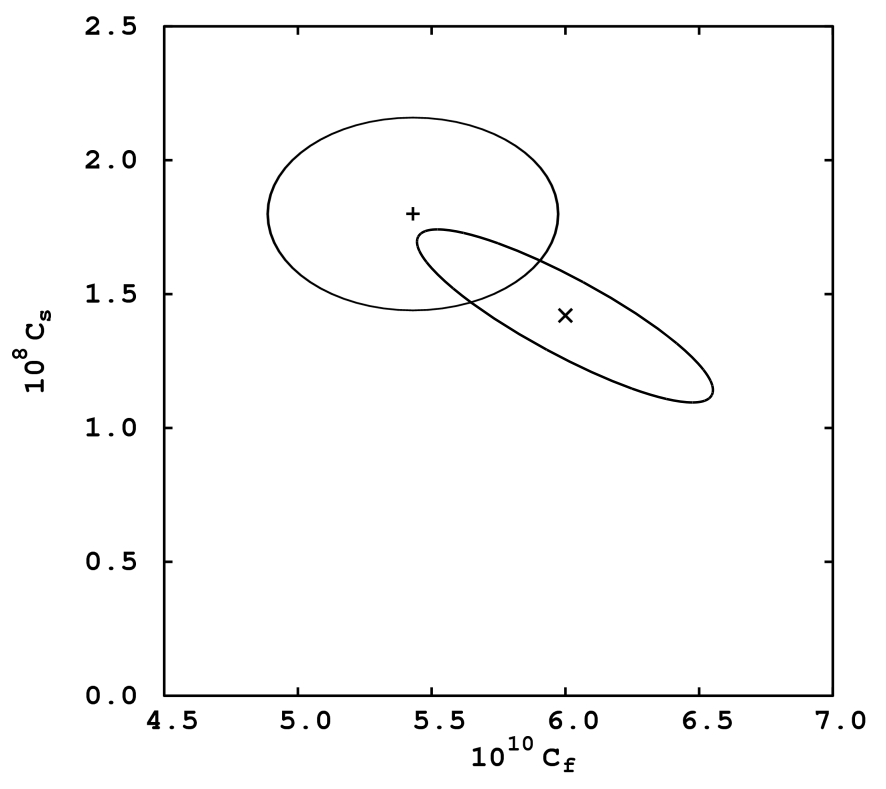
Figure A1Cs vs. Cf for the R98 model (+) and its modification by Turner et al. (2009) (×), with uncertainty contours. Note the different scales on the two axes.
Parameters for higher-frequency lines (321–916 GHz) were modified according to different sets of spectroscopic measurements (Colmont et al., 1999; Podobedov et al., 2004; Koshelev et al., 2007; Golubiatnikov et al., 2008; Koshelev, 2011; Tretyakov et al., 2013), leading to modifications in air-broadened line width (order of 1 %–15 %), the temperature exponent of air broadening (2 %–5 %), and self-broadened line width (1 %–9 %). Other line parameters are from the HITRAN 2012 database (Rothman et al., 2013).
Concerning the water vapor continuum, the main modifications follow the results of Turner et al. (2009) suggested by an analysis of ground-based observations at 150 GHz. The suggested adjustments to the two components of the water vapor continuum in the R98 model are in opposite directions (i.e., increasing the contribution from the foreign-broadened component while decreasing the contribution from the self-broadened component). Figure A1 plots Cs vs. Cf for the R98 model and its modification by Turner et al. (2009) with their respective uncertainty contours. These uncertainties are conditioned on the nominal values of ncs and ncf, which are the same in both models. The uncertainty ellipse for Turner et al. is drawn using the correlation coefficient of −0.87 found in Sect. 4.1.3. Note that the details of continuum and resonant absorption are inextricably related in any model, meaning that the empirical definition of the continuum (Eq. 8) implies that the parameters must be used only with exactly the same resonance absorption they were defined with. Thus, the adjustment factors were recomputed in 2015 accounting for the resonant line adjustments discussed above, leading to +9.8 % and −21.1 % change from R98 in air-broadened and self-broadened coefficients, respectively. The results of Turner et al. (2009) are indirectly supported by the analysis of Payne et al. (2011). In fact, Payne et al. (2011) developed adjustment factors for the MT_CKD water vapor continuum model (Clough et al., 2005; Mlawer et al., 2012), which agree within the stated error bars with those given in Turner et al. (2009) for the same MT_CKD model. The results of Turner et al. (2009) also seem supported by independent investigations based on satellite observations in the 10.7 to 89 GHz range (Wentz and Meissner, 2016) and around the 183 GHz line (Bobryshev et al., 2018).
More recently, two papers presented further modifications to the spectroscopy underlying microwave remote sensing of atmospheric water vapor, i.e., Tretyakov (2016) and Koshelev et al. (2018). Tretyakov (2016) presents a historic review, discussing in chronological order the measurement and analysis that lead to estimates of spectroscopic parameters for the water vapor absorption continuum and resonant lines near 22 and 183 GHz. Tretyakov (2016) also provides an expert assessment of the best estimate for the spectroscopic parameter values and their uncertainty based on the analysis of all the available data. These parameter values provide the best fit of the absorption model to the available data, taking into account the measurement errors reported by the authors and the probabilities of possible systematic errors. In almost all cases, with the exception of the 22 GHz line self-broadening, the estimated parameter values agree within uncertainty limits with those given in HITRAN, though in most cases HITRAN uncertainty estimates are more conservative. Concerning the water vapor continuum absorption, Tretyakov (2016) finds that the adjustments to R98 proposed by Turner et al. (2009), based on zenith-looking ground-based radiometric observation, lead to a worse fit to the laboratory and field (parallel to Earth-surface path) measurements, particularly noticeable in the self component. However, Fig. A1 shows that the model uncertainties have appreciable overlap. Finally, Koshelev et al. (2018) present laboratory measurements devoted to refining the 22 GHz line-shape parameters. Koshelev et al. (2018) suggest line width values within the uncertainty of those given by Tretyakov (2016), though with smaller estimated uncertainty by a factor of ∼3 (air broadening) and ∼10 (self-broadening). Similarly, the air-broadening shift parameter agrees with that of Tretyakov (2016) with an estimated uncertainty reduced by a factor of ∼3. Conversely, the uncertainty of the self-broadening shift parameter is reduced by a factor ∼1.5, and the values from Tretyakov (2016) and Koshelev et al. (2018) do not fit within the stated uncertainty.
A2 Oxygen
The R98 model adopts the same oxygen line parameters as given in MPM92, except for sub-millimeter frequencies for which frequency and intensity are taken from the HITRAN 1992 database (Rothman et al., 1992). Other differences with respect to MPM92 are the temperature dependence (1∕T) for 118.75 GHz line width, with the temperature dependence of sub-millimeter line widths being equal to that of lines in the 60 GHz band (e.g., , with na=0.8). Concerning the line-mixing model, the MPM and the R98 model exploit first-order mixing with coefficients derived by the method given in Rosenkranz (1988). The following modifications have been implemented in R17.
The line intensities are from the HITRAN 2004 database (Rothman et al., 2005). The zero-frequency line intensity is from the JPL catalogue (https://spec.jpl.nasa.gov/; Pickett et al., 1998). The line central frequencies and width coefficients for the 60 GHz band are taken from Tretyakov et al. (2005), who report measurements for precise broadening and central frequencies of fine structure lines and a revision of line-mixing coefficients. The effect of different values for the 60 GHz line parameters on MWR simulations and retrievals was shown to be significant both for ground-based (Cadeddu et al., 2007) and satellite (Boukabara et al., 2005a, b; Rosenkranz, 2005) observations. In particular, Cadeddu et al. (2007) show that the parameter values proposed by Tretyakov et al. (2005) lead to better agreement with two independent datasets of ground-based MWR observations than those found in HITRAN (Rothman et al., 2005; Hoke et al., 1989) and also that these modifications are essential to reduce the clear-sky bias in the liquid–water path retrievals.
The line width and line-mixing coefficients for the 118 GHz line are taken from Tretyakov et al. (2004), who report results of laboratory investigations of the pressure-dependent parameters of the single 118 GHz line. The sub-millimeter line widths are from Golubiatnikov and Krupnov (2003), except the one at the 234 GHz line that comes from Drouin (2007).
Makarov et al. (2011) proposed a model for the 60 GHz absorption band based on the second-order line-mixing expansion of Smith (1981), showing an improved fit of observed absorption profiles between 54 and 65 GHz, but this model is not adopted in R17. In fact, during this analysis, significant absorption differences (∼10 %) were found in the band wings (e.g., ∼50–53 GHz) comparing calculations made with Makarov et al. (2011) line-mixing coefficients against original measurements from Liebe et al. (1992). This was attributed to systematic errors in O2 concentration of the order of 0.5 %–1.5 % in the 245–335 K temperature range. Dmitriy S. Makarov, Philip W. Rosenkranz, and Mikhail Y. Tretyakov are currently working on a revised second-order model (Makarov et al., 2018).
For the dry continuum, R98 only considered the N2–N2 contribution with a pure ν2 dependence. This is a particular case of Eqs. (7) and (15), with and f(ν)=1. This was revised (Rosenkranz et al., 2006) by fitting f(ν) as in Eq. (16) through the data of Borysow and Frommhold (1986) and including the N2–O2 and O2–O2 bimolecular absorption with a constant value for ε suggested by Pardo et al. (2001) and later by Boissoles et al. (2003). The latter is used in R17.
In order to consider the broadening of oxygen lines by water vapor with little modifications to the original model, R17 adopts the mean value of the water-to-air broadening ratio suggested by Koshelev et al. (2015).
More recently, Koshelev et al. (2016) report measurements of line widths and their temperature exponents for 12 oxygen lines (rotational quantum number N ranging from 1 to 19). The fixed value of the temperature exponent (na=0.8) adopted in the MPM and the R98–R17 models fits the value reported in Makarov et al. (2008) for the 1− line (0.785(35)) but falls outside the mean value (0.765(11)) reported by Koshelev et al. (2016). This suggests that the temperature exponent values suggested by Koshelev et al. (2016), or their mean value, could be adopted to increase the accuracy of absorption modeling.
The supplement related to this article is available online at: https://doi.org/10.5194/acp-18-15231-2018-supplement.
DC and PR designed the research, contributed to data processing and analysis, and wrote the original manuscript. MYT, MAK, and FR provided advice and contributed to data analysis. All the co-authors helped to revise the manuscript.
The authors declare that they have no conflict of interest.
This work was partially supported by the EU H2020 project GAIA-CLIM
(Ares(2014)3708963, project 640276). Mikhail Y. Tretyakov and Maksim A. Koshelev acknowledge
state project no. 0035-2014-009. Domenico Cimini acknowledges the useful
advice from Stefan Bühler, Richard Larsson, and Oliver Lemke in the early
stage of the analysis.
Edited by: Jui-Yuan Christine Chiu
Reviewed by: Vivienne Payne and two anonymous referees
Alvarado, M. J., Payne, V. H., Mlawer, E. J., Uymin, G., Shephard, M. W., Cady-Pereira, K. E., Delamere, J. S., and Moncet, J.-L.: Performance of the Line-By-Line Radiative Transfer Model (LBLRTM) for temperature, water vapor, and trace gas retrievals: recent updates evaluated with IASI case studies, Atmos. Chem. Phys., 13, 6687–6711, https://doi.org/10.5194/acp-13-6687-2013, 2013.
Alvarado, M. J., Payne, V. H., Cady-Pereira, K. E., Hegarty, J. D., Kulawik, S. S., Wecht, K. J., Worden, J. R., Pittman, J. V., and Wofsy, S. C.: Impacts of updated spectroscopy on thermal infrared retrievals of methane evaluated with HIPPO data, Atmos. Meas. Tech., 8, 965–985, https://doi.org/10.5194/amt-8-965-2015, 2015.
Bauer, A., Godon, M., Kheddar, M., and Hartmann, J. M.: Temperature and perturber dependences of water vapor line-broadening. Experiments at 183 GHz calculations below 1000 GHz, J. Quant. Spectrosc. Ra., 41, 49–54, https://doi.org/10.1016/0022-4073(89)90020-4, 1989.
Bobryshev, O., Buehler, S. A., John, V. O., Brath, M., and Brogniez, H.: Is there really a closure gap between 183.31 GHz satellite passive microwave and in-situ radiosonde water vapor measurements?, IEEE T. Geosci. Remote, 56, 1–7, https://doi.org/10.1109/TGRS.2017.2786548, 2018.
Bodeker, G. E., Bojinski, S., Cimini, D., Dirksen, R. J., Haeffelin, M., Hannigan, J. W., Hurst, D., Madonna, F., Maturilli, M., Mikalsen, A. C., Philipona, R., Reale, T., Seidel, D. J., Tan, D. G. H., Thorne, P. W., Vömel, H., and Wang, J.: Reference upper-air observations for climate: From concept to reality, B. Am. Meteorol. Soc., 97, 123–135, https://doi.org/10.1175/BAMS-D-14-00072.1, 2015.
Boissoles, J., Boulet, C., Tipping, R. H., Brown, A., and Ma, Q.: Theoretical calculation of the translation-rotation collision-induced absorption in N2–N2, O2–O2, and N2–O2 pairs, J. Quant. Spectrosc. Ra., 82, 505–516, https://doi.org/10.1016/S0022-4073(03)00174-2, 2003.
Borysow, A. and Frommhold, L.: Collision-Induced Rototranslational Absorption Spectra of N2-N2 Pairs for Temperatures from 50 To 300 K, Astrophys. J., 311, 1043–1057, https://doi.org/10.1086/164841, 1986.
Boukabara, S. A., Clough, S. A., Moncet, J.-L., Krupnov, A. F., Tretyakov, M. Yu., and Parshin, V. V.: Uncertainties in the Temperature Dependence of the Line-Coupling Parameters of the Microwave Oxygen Band: Impact Study, IEEE T. Geosci. Remote, 43, 1109–1114, https://doi.org/10.1109/TGRS.2004.839654, 2005a.
Boukabara, S. A., Clough, S. A., Moncet, J.-L., Krupnov, A. F., Tretyakov, M. Yu., and Parshin, V. V.: Reply to the Comment on “Uncertainties in the Temperature Dependence of the Line-Coupling Parameters of the Microwave Oxygen Band: Impact Study”, IEEE T. Geosci. Remote, 43, 2161–2162, https://doi.org/10.1109/TGRS.2005.853188, 2005b.
Brogniez, H., English, S., Mahfouf, J.-F., Behrendt, A., Berg, W., Boukabara, S., Buehler, S. A., Chambon, P., Gambacorta, A., Geer, A., Ingram, W., Kursinski, E. R., Matricardi, M., Odintsova, T. A., Payne, V. H., Thorne, P. W., Tretyakov, M. Yu., and Wang, J.: A review of sources of systematic errors and uncertainties in observations and simulations at 183 GHz, Atmos. Meas. Tech., 9, 2207–2221, https://doi.org/10.5194/amt-9-2207-2016, 2016.
Buehler, S. A., Eriksson, P., Kuhn, T., von Engeln, A., and Verdes, C.: ARTS, the Atmospheric Radiative Transfer Simulator, J. Quant. Spectrosc. Ra., 91, 65–93, https://doi.org/10.1016/j.jqsrt.2004.05.051, 2005.
Cadeddu, M., Payne, V. H., Clough, S. A., Cady-Pereira, K., and Liljegren, J. C.: The effect of the oxygen line-parameter modeling on temperature and humidity retrievals from ground-based microwave radiometers, IEEE T. Geosci. Remote, 45, 2216– 2223, https://doi.org/10.1109/TGRS.2007.894063, 2007.
Cazzoli, G., Puzzarini, C., Buffa, G., and Tarrini O.: Experimental and theoretical investigation on pressure-broadening and pressure-shifting of the 22.2 GHz line of water, J. Quant. Spectrosc. Ra., 105, 438–449, https://doi.org/10.1016/j.jqsrt.2006.11.003, 2007.
Colmont, J.-M., Priem, D., Wlodarczak, G., and Gamache, R. R.: Measurements and Calculations of the Halfwidth of Two Rotational Transitions of Water Vapor Perturbed by N2, O2, and Air, J. Mol. Spectrosc., 193, 233–243, https://doi.org/10.1006/jmsp.1998.7747, 1999.
Connor, B., Bösch, H., McDuffie, J., Taylor, T., Fu, D., Frankenberg, C., O'Dell, C., Payne, V. H., Gunson, M., Pollock, R., Hobbs, J., Oyafuso, F., and Jiang, Y.: Quantification of uncertainties in OCO-2 measurements of XCO2: simulations and linear error analysis, Atmos. Meas. Tech., 9, 5227–5238, https://doi.org/10.5194/amt-9-5227-2016, 2016.
Cimini, D., Westwater, E. R., Ware, R., Keihm, S. J., Han, Y., Marzano, F. S., and Ciotti, P.: Empirical evaluation of four microwave radiative forward models based on ground-based radiometer between 20 and 60 GHz, Proc. 14th ARM Science Team Meeting, 2004.
Cimini, D., Hewison, T. J., Martin, L., Güldner, J., Gaffard, C., and Marzano, F. S.: Temperature and humidity profile retrievals from ground-based microwave radiometers during TUC, Meteorol. Z., 15, 45–56, https://doi.org/10.1127/0941-2948/2006/0099, 2006.
Cimini, D., Westwater, E. R., and Gasiewski, A. J.: Temperature and humidity profiling in the Arctic using ground-based millimeter-wave radiometry and 1DVAR, IEEE T. Geosci. Remote, 48, 1381–1388, https://doi.org/10.1109/TGRS.2009.2030500, 2010.
Cimini, D., Rosenkranz, P. W., Tretyakov, M. Yu., Koshelev, M. A., and Romano, F.: Sensitivity of microwave downwelling brightness temperatures to spectroscopic parameter uncertainty, Proc. of International TOVS Study Conference, Darmstadt, Germany, 29 November–5 December, available at: http://cimss.ssec.wisc.edu/itwg/itsc/itsc21/proceedings/2p.08_cimini.pdf (last access: 22 May 2018), 2017.
Clough, S. A., Kneizys, F. X., and Davies, R. W.: Line shape and the water vapor continuum, Atmos. Res., 23, 229–241, https://doi.org/10.1016/0169-8095(89)90020-3, 1989.
Clough, S. A., Shephard, M. W., Mlawer, E. J., Delamere, J. S., Iacono, M. J., Cady-Pereira, K., Boukabara, S., and Brown, P. D.: Atmospheric radiative transfer modeling: a summary of the AER codes, J. Quant. Spectrosc. Ra., 9, 233–244, https://doi.org/10.1016/j.jqsrt.2004.05.058, 2005.
Danese, L. and Partridge, R. B.: Atmospheric emission models – Confrontation between observational data and predictions in the 2.5–300 GHz frequency range, Astrophys. J., 342, 604–615, https://doi.org/10.1086/167620, 1989.
De Angelis, F., Cimini, D., Hocking, J., Martinet, P., and Kneifel, S.: RTTOV-gb – adapting the fast radiative transfer model RTTOV for the assimilation of ground-based microwave radiometer observations, Geosci. Model Dev., 9, 2721–2739, https://doi.org/10.5194/gmd-9-2721-2016, 2016.
Dirksen, R. J., Sommer, M., Immler, F. J., Hurst, D. F., Kivi, R., and Vömel, H.: Reference quality upper-air measurements: GRUAN data processing for the Vaisala RS92 radiosonde, Atmos. Meas. Tech., 7, 4463–4490, https://doi.org/10.5194/amt-7-4463-2014, 2014.
Drouin, B. J.: Temperature dependent pressure induced linewidths of 16O2 and 18O16O transitions in nitrogen, oxygen and air, J. Quant. Spectrosc. Ra., 105, 450–458, https://doi.org/10.1016/j.jqsrt.2006.12.001, 2007.
Eriksson, P., Buehler, S. A., Davis, C. P., Emde, C., and Lemke, O.: ARTS, the atmospheric radiative transfer simulator, Version 2, J. Quant. Spectrosc. Ra., 112, 1551–1558, https://doi.org/10.1016/j.jqsrt.2011.03.001, 2011.
GAIA-CLIM, Gaps Assessment and Impacts Document (GAID) – G2.37: Poorly quantified uncertainties in spectroscopic information, available at: http://www.gaia-clim.eu/system/files/document/d6.11.pdf (last access: 15 October 2018), 2017.
Gamache, R. R., Roller, C., Lopes, E., Gordon, I. E., Rothman, L. S., Polyansky, O. L., Zobov, N. F., Kyuberis, A. A., Tennyson, J., Yurchenko, S. N., Császár, A. G., Furtenbacher, T., Huang, X., Schwenke, D. W., Lee, T. J., Drouin, B. J., Tashkun, S. A., Perevalov, V. I., and Kochanov, R. V.: Total internal partition sums for 166 isotopologues of 51 molecules important in planetary atmospheres: Application to HITRAN2016 and beyond, J. Quant. Spectrosc. Ra., 203, 70–87, https://doi.org/10.1016/j.jqsrt.2017.03.045, 2017.
Golubiatnikov, G. Yu.: Shifting and broadening parameters of the water vapor 183-GHz line (313–220) by H2O, O2, N2, CO2, H2, He, Ne, Ar, and Kr at room temperature, J. Mol. Spectrosc., 230, 196–198, https://doi.org/10.1016/j.jms.2004.10.011, 2005.
Golubiatnikov, G. Y. and Krupnov, A. F.: Microwave study of the rotational spectrum of oxygen molecule in the range up to 1.12 THz, J. Mol. Spectrosc., 217, 282–287, https://doi.org/10.1016/S0022-2852(02)00058-9, 2003.
Golubiatnikov, G. Yu., Markov, V. N., Guarnieri, A., and Knöchel, R.: Hyperfine structure of and measured by Lamb-dip technique in the 180–560 GHz frequency range, J. Mol. Spectrosc., 240, 251–254, https://doi.org/10.1016/j.jms.2006.09.012, 2006.
Golubiatnikov, G. Yu., Koshelev, M. A., and Krupnov, A. F.: Pressure shift and broadening of 110–101 water vapor lines by atmosphere gases, J. Quant. Spectrosc. Ra., 109, 1828–1833, https://doi.org/10.1016/j.jqsrt.2007.12.006, 2008.
Gordon, I. E., Rothman, L. S., Hill, C., Kochanov, R. V., Tan, Y., Bernath, P. F., Birk, M., Boudon, V., Campargue, A., Chance, K. V., Drouin, B. J., Flaud, J.-M., Gamache, R. R., Hodges, J. T., Jacquemart, D., Perevalov, V. I., Perrin, A., Shine, K. P., Smith, M.-A. H., Tennyson, J., Toon, G. C., Tran, H., Tyuterev, V. G., Barbe, A., Császár, A. G., Devi, V. M., Furtenbacher, T., Harrison, J. J., Hartmann, J.-M., Jolly, A., Johnson, T. J., Karman, T., Kleiner, I., Kyuberis, A. A., Loos, J., Lyulin, O. M., Massie, S. T., Mikhailenko, S. N., Moazzen-Ahmadi, N., Müller, H. S. P., Naumenko, O. V., Nikitin, A. V., Polyansky, O. L., Rey, M., Rotger, M., Sharpe, S. W., Sung, K., Starikova, E., Tashkun, S. A., Vander Auwera, J., Wagner, G., Wilzewski, J., Wcisło, P., Yu, S., and Zak, E. J.: The HITRAN2016 molecular spectroscopic database, J. Quant. Spectrosc. Ra., 203, 3–69, https://doi.org/10.1016/j.jqsrt.2017.06.038, 2017.
Hewison, T. J.: Aircraft Validation of Clear Air Absorption Models at Millimeter Wavelengths (89–183 GHz), J. Geophys. Res., 111, D14303, https://doi.org/10.1029/2005JD006719, 2006a.
Hewison, T. J.: Profiling Temperature and Humidity by Ground-based Microwave Radiometers, PhD Thesis, Department of Meteorology, University of Reading, 2006b.
Hewison, T. J.: 1D-VAR retrievals of temperature and humidity profiles from a ground-based microwave radiometer, IEEE T. Geosci. Remote, 45, 2163–2168, https://doi.org/10.1109/TGRS.2007.898091, 2007.
Hewison, T. J., Cimini, D., Martin, L., Gaffard, C., and Nash, J.: Validating clear air absorption model using ground-based microwave radiometers and vice-versa, Meteorol. Z., 15, 27–36, 2006.
Hill, R. J.: Water vapor-absorption line shape comparison using the 22-GHz line: The Van Vleck-Weisskopf shape affirmed, Radio Sci., 21, 447–451, https://doi.org/10.1029/RS021i003p00447, 1986.
Ho, W., Wang, H. H., Hall, W. F., Norris, W., Hardy, W. N., Gray, K. W., and Hidy, G. M.: Brightness Temperature of the Terrestrial Sky at 2.66 GHz, J. Atmos. Sci., 29, 1210–1212, https://doi.org/10.1175/1520-0469(1972)029<1210:BTOTTS>2.0.CO;2, 1972.
Hoke, M. L., Clough, S. A., Lafferty, W. J., and Olson, B. W.: Line cou- pling in oxygen and carbon dioxide, in IRS 88: Current Problems in Atmospheric Radiation, edited by: Lenoble, J. and Geleyn, J. F., Hampton, VA, A. Deepak, 368–371, 1989.
Joint Committee for Guides in Metrology (JCGM): Evaluation of Measurement Data – Guide to the Expression of Uncertainty in Measurement, available at: https://www.bipm.org/utils/common/documents/jcgm/JCGM_100_2008_E.pdf (last access: 25 May 2018), 2008.
Kaufman, I. A.: Microwave pressure broadening in O2 and H2O above one atmosphere, PhD thesis, Columbia Univ., New York, 1967.
Koshelev, M. A.: Collisional broadening and shifting of the 211–202 transition of , , by atmosphere gases, J. Quant. Spectrosc. Ra., 112, 550–552, https://doi.org/10.1016/j.jqsrt.2010.10.009, 2011.
Koshelev, M. A., Tretyakov, M. Yu., Golubiatnikov, G. Yu., Parshin, V. V., Markov, V. N., and Koval, I. A.: Broadening and shifting of the 321-, 325- and 380-GHz lines of water vapor by pressure of atmospheric gases, J. Mol. Spectrosc., 241, 101–108, https://doi.org/10.1016/j.jms.2006.11.005, 2007.
Koshelev, M. A., Serov, E. A., Parshin, V. V., and Tretyakov, M. Yu.: Millimeter wave continuum absorption in moist nitrogen at temperatures 261–328 K, J. Quant. Spectrosc. Ra., 112, 2704–2712, https://doi.org/10.1016/j.jqsrt.2011.08.004, 2011.
Koshelev, M. A., Vilkov, I. N., and Tretyakov, M. Yu.: Pressure broadening of oxygen fine structure lines by water, J. Quant. Spectrosc. Ra., 154, 24–27, https://doi.org/10.1016/j.jqsrt.2014.11.019, 2015.
Koshelev, M. A., Vilkov, I. N., and Tretyakov, M. Yu.: Collisional broadening of oxygen fine structure lines: The impact of temperature, J. Quant. Spectrosc. Ra., 169, 91–95, https://doi.org/10.1016/j.jqsrt.2015.09.018, 2016.
Koshelev, M. A., Golubiatnikov, G. Yu., Vilkov, I. N., and Tretyakov, M. Yu.: Line shape parameters of the 22-GHz water line for accurate modeling in atmospheric applications, J. Quant. Spectrosc. Ra., 205, 51–58, https://doi.org/10.1016/j.jqsrt.2017.09.032, 2018.
Kuhn, T., Bauer, A., Godon, M., Buehler, S., and Kunzi, K.: Water vapor continuum: absorption measurements at 350 GHz and model calculations, J. Quant. Spectrosc. Ra., 74, 545–562, https://doi.org/10.1016/S0022-4073(01)00271-0, 2002.
Kukolich, S. G.: Measurement of the Molecular g Values in H2O and D2O and Hyperfine Structure in H2O, J. Chem. Phys., 50, 3751–3755, https://doi.org/10.1063/1.1671623, 1969.
Liebe, H. J.: MPM – An atmospheric millimeter wave propagation model, Int. J. Infrared Milli., 10, 631–650, https://doi.org/10.1007/BF01009565, 1989.
Liebe, H. J. and Layton, D. H.: Millimeter-wave properties of the atmosphere: Laboratory studies and propagation modeling, NTIA Rep. 87-224, National Telecommunication and Information Administration, Boulder, CO, 1987.
Liebe, H. J., Rosenkranz, P. W., and Hufford, G. A.: Atmospheric 60-GHz oxygen spectrum: New laboratory measurements and line parameters, J. Quant. Spectrosc. Ra., 45, 629–643, 1992 (dataset available at: https://www.its.bldrdoc.gov/media/66297/liebe_data.zip).
Liebe, H. J., Hufford, G. A., and Cotton, M. G.: Propagation modeling of moist air and suspended water/ice particles at frequencies below 1000 GHz, Proc. NATO/AGARD Wave Propagation Panel, 52nd meeting, No. 3/1-10, Mallorca, Spain, 17–20 May 1993.
Liljegren, J. C., Boukabara, S. A., Cady-Pereira, K., and Clough, S. A.: The effect of the half-width of the 22-GHz water vapor line on retrievals of temperature and water vapor profiles with a twelve-channel microwave radiometer, IEEE T. Geosci. Remote, 43, 1102–1108, https://doi.org/10.1109/TGRS.2004.839593, 2005.
Löhnert, U., Crewell, S., and Simmer, C.: An integrated approach toward retrieving physically consistent profiles of temperature, humidity, and cloud liquid water, J. Appl. Meteorol., 43, 1295–1307, https://doi.org/10.1175/1520-0450(2004)043<1295:AIATRP>2.0.CO;2, 2004.
Long, D. A. and Hodges, J. T.: On spectroscopic models of the O2 A-band and their impact upon atmospheric retrievals, J. Geophys. Res., 117, D12309, https://doi.org/10.1029/2012JD017807, 2012.
Makarov, D. S., Koval, I. A., Koshelev, M. A., Parshin, V. V., and Tretyakov, M. Yu.: Collisional parameters of the 118 GHz oxygen line: temperature dependence, J. Mol. Spectrosc., 252, 242–243, https://doi.org/10.1016/j.jms.2008.08.005, 2008.
Makarov, D. S., Tretyakov, M. Yu., and Rosenkranz, P. W.: 60-GHz oxygen band: Precise experimental profiles and extended absorption modeling in a wide temperature range, J. Quant. Spectrosc. Ra., 112, 1420–1428, https://doi.org/10.1016/j.jqsrt.2011.02.018, 2011.
Makarov, D. S., Tretyakov, M. Yu., and Boulet, C.: Line mixing in the 60-GHz atmospheric oxygen band: Comparison of the MPM and ECS model, J. Quant. Spectrosc. Ra., 124, 1–10, https://doi.org/10.1016/j.jqsrt.2013.02.019, 2013.
Melsheimer, C., Verdes, C., Buehler, S. A., Emde, C., Eriksson, P., Feist, D. G., Ichizawa, S., John, V. O., Kasai, Y., Kopp, G., Koulev, N., Kuhn, T., Lemke, O., Ochiai, S., Schreier, F., Sreerekha, T. R., Suzuki, M., Takahashi, C., Tsujimaru, S., and Urban, J.: Intercomparison of general purpose clear sky atmospheric radiative transfer models for the millimeter/submillimeter spectral range, Radio Sci., 40, RS1007, https://doi.org/10.1029/2004RS003110, 2005.
Ma, Q., Boulet, C., and Tipping, R. H.: Effects on calculated half-widths and shifts from the line coupling for asymmetric-top molecules, J. Chem. Phys., 140, 244301, https://doi.org/10.1063/1.4883058, 2014.
Makarov, D. S., Tretyakov, M. Yu., and Rosenkranz, P. W.: Atmospheric oxygen mm-absorption: models review and uncertainties evaluation, 25th International Conference on High Resolution Molecular Spectroscopy, 3–7 September, report A7.4, book of abstracts, Bilbao, Spain, p. 136, 2018.
Martinet, P., Dabas, A., Donier, J. M., Douffet, T., Garrouste, O., and Guillot, R.: 1D-Var temperature retrievals from microwave radiometer and convective scale model, Tellus A, 67, 27925, https://doi.org/10.3402/tellusa.v67.27925, 2015.
Martinet, P., Cimini, D., De Angelis, F., Canut, G., Unger, V., Guillot, R., Tzanos, D., and Paci, A.: Combining ground-based microwave radiometer and the AROME convective scale model through 1DVAR retrievals in complex terrain: an Alpine valley case study, Atmos. Meas. Tech., 10, 3385–3402, https://doi.org/10.5194/amt-10-3385-2017, 2017.
Maschwitz, G., Löhnert, U., Crewell, S., Rose, T., and Turner, D. D.: Investigation of ground-based microwave radiometer calibration techniques at 530 hPa, Atmos. Meas. Tech., 6, 2641–2658, https://doi.org/10.5194/amt-6-2641-2013, 2013.
Mätzler, C.: Development of Radiative Transfer Models, Report from Review Workshop of Project 1 of COST Action 712 Application of microwave radiometry to atmospheric research and monitoring, edited by: Mätzler, C., EUMETSAT, Am Kavalleriesand 31, 64295 Darmstadt, Germany, 8–10 April 1997.
Mlawer, E. J., Payne, V. H., Moncet, J.-L., Delamere, J. S., Alvarado, M. J., and Tobin, D. C.: Development and recent evaluation of the MT_CKD model of continuum absorption, Philos. T. R. Soc. A, 2012, 2520–2556, https://doi.org/10.1098/rsta.2011.0295, 2012.
Pardo, J. R., Serabyn, E., and Cernicharo, J.: Submillimeter atmospheric transmission measurements on Mauna Kea during extremely dry El Nino conditions: implications for broadband opacity contributions, J. Quant. Spectrosc. Ra., 68, 419–433, https://doi.org/10.1016/S0022-4073(00)00034-0, 2001.
Payne, V. H., Delamere, J. S., Cady-Pereira, K. E., Gamache, R. R., Moncet, J.-L., Mlawer, E. J., and Clough, S. A.: Air-broadened halfwidths of the 22 GHz and 183 GHz water vapor lines, IEEE T. Geosci. Remote, 46 3601–3617, https://doi.org/10.1109/TGRS.2008.2002435, 2008.
Payne, V. H., Mlawer, E. J., Cady-Pereira, K. E., and Moncet, J.-L.: Water vapor continuum absorption in the microwave, IEEE T. Geosci. Remote, 49, 2194–2208, https://doi.org/10.1109/TGRS.2010.2091416, 2011.
Pickett, H. M.: Effects of velocity averaging on the shapes of absorption lines, J. Chem. Phys. 73, 6090–6094, https://doi.org/10.1063/1.440145, 1980.
Pickett, H. M., Poynter, R. L., Cohen, E. A., Delitsky, M. L., Pearson, J. C., and Muller, H. S. P.: Submillimeter, Millimeter, and Microwave Spectral Line Catalog, J. Quant. Spectrosc. Ra., 60, 883–890, https://doi.org/10.1016/S0022-4073(98)00091-0, 1998.
Podobedov, V. B., Plusquellic, D. F., and Fraser, G. T.: THz laser study of self-pressure and temperature broadening and shifts of water vapor lines for pressures up to 1.4 kPa, J. Quant. Spectrosc. Ra., 87, 377–385, https://doi.org/10.1016/j.jqsrt.2004.03.001, 2004.
Polyansky, O. L., Kyuberis, A. A., Zobov, N. F., Tennyson, J., Yurchenko, S. N., and Lodi, L.: ExoMol molecular line lists XXX: a complete high-accuracy line list for water, Monthly Not. R. Astron. Soc., 480, 2597–2608, https://doi.org/10.1093/mnras/sty1877, 2018.
Rayer, P. J.: Microwave transmittance models for RTTOV, report, Met Office, Exeter, UK, available at: https://www.nwpsaf.eu/site/download/documentation/rtm/papers/rpt_rayer.pdf (last access: 10 January 2018), 2001.
Rodgers C. D.: Inverse Methods for Atmospheric Sounding: Theory and Practise, vol. 2, Series on Atmospheric, Oceanic and Planetary Physics, World Scientific, Singapore, ISBN: 978-981-02-2740-1, 2000.
Rose, T., Crewell, S., Löhnert, U., and Simmer, C.: A network suitable microwave radiometer for operational monitoring of the cloudy atmosphere, Atmos. Res., 75, 183–200, https://doi.org/10.1016/j.atmosres.2004.12.005, 2005.
Rosenkranz, P. W.: Shape of the 5 mm oxygen band in the atmosphere, IEEE T. Antenn. Propag., 23, 498–506, https://doi.org/10.1109/TAP.1975.1141119, 1975.
Rosenkranz, P. W.: Interference coefficients for overlapping oxygen lines in air, J. Quant. Spectrosc. Ra., 39, 287–297, https://doi.org/10.1016/0022-4073(88)90004-0, 1988.
Rosenkranz, P. W.: Absorption Of Microwaves By Atmospheric Gases, chap. 2, in: Atmospheric Remote Sensing by Microwave Radiometry, edited by: Janssen, M. A., New York, J. Wiley & Sons, Inc., 37–90, http://hdl.handle.net/1721.1/68611, 1993.
Rosenkranz, P. W.: Water vapor microwave continuum absorption: A comparison of measurements and models, Radio Sci., 33, 919–928, https://doi.org/10.1029/98RS01182, 1998.
Rosenkranz, P. W.: Retrieval of Temperature and Moisture Profiles From AMSU-A and AMSU-B Measurements, IEEE T. Geosci. Remote, 39, 2429–2435, https://doi.org/10.1109/36.964979, 2001.
Rosenkranz, P. W.: Comment on “Uncertainties in the temperature dependence of the line-coupling parameters of the microwave oxygen band: impact study”, IEEE T. Geosci. Remote, 43, 2160–2161, https://doi.org/10.1109/TGRS.2005.853189, 2005.
Rosenkranz, P. W.: Line-by-line microwave radiative transfer (non-scattering), Remote Sens. Code Library, https://doi.org/10.21982/M81013, 2017.
Rosenkranz, P. W. and Barnet, C. D.: Microwave radiative transfer model validation, J. Geophys. Res., 111, D09S07, https://doi.org/10.1029/2005JD006008, 2006.
Rosenkranz, P. W., Buehler, S. A., Feist, D. G., Hewison, T. J., Jacquinet-Husson, N., Pardo, J. R., and Saunders, R.: Emission and spectroscopy of the clear atmosphere, chap. 2, in: Thermal Microwave Radiation: Applications for Remote Sensing, edited by: Mätzler, C., London, IET, 2006.
Rosenkranz, P. W., Cimini, D., Koshelev, M. A., and Tretyakov, M. Yu.: Covariances of Spectroscopic Parameter Uncertainties in Microwave Forward Models and Consequences for Remote Sensing, 2018 IEEE 15th Specialist Meeting on Microwave Radiometry and Remote Sensing of the Environment (MicroRad), Cambridge, MA, USA, 1–6, https://doi.org/10.1109/MICRORAD.2018.8430729, 2018.
Rothman, L. S., Gamache, R. R., Tipping, R. H., Rinsland, C. P., Smith, M. A. H., Chris Benner, D., Malathy Devi, V., Flaud, J.-M., Camy-Peyret, C., Perrin, A., Goldman, A., Massie, S. T., Brown, L. R., and Toth, R. A.: The HITRAN molecular database: Editions of 1991 and 1992, J. Quant. Spectrosc. Ra., 48, 469–507, https://doi.org/10.1016/0022-4073(92)90115-K, 1992.
Rothman, L. S., Jacquemart, D., Barbe, A., Chris Benner, D., Birk, M., Brown, L. R., Carleer, M. R., Chackerian, C., Chance, K., Coudert, L. H., Dana, V., Devi, V. M., Flaud, J.-M., Gamache, R. R., Goldman, A., Hartmann, J.-M., Jucks, K. W., Maki, A. G., Mandin, J.-Y., Massie, S. T., Orphal, J., Perrin, A., Rinsland, C. P., Smith, M. A. H., Tennyson, J., Tolchenov, R. N., Toth, R. A., Vander Auwera, J., Varanasi, P., and Wagner, G.: The HITRAN 2004 molecular spectroscopic database, J. Quant. Spectrosc. Ra., 96, 139–204, https://doi.org/10.1016/j.jqsrt.2004.10.008, 2005.
Rothman, L. S., Gordon, I. E., Babikov, Y., Barbe, A., Chris Benner, D., Bernath, P. F., Birk, M., Bizzocchi, L., Boudon, V., Brown, L. R., Campargue, A., Chance, K., Cohen, E. A., Coudert, L. H., Devi, V. M., Drouin, B. J., Fayt, A., Flaud, J.-M., Gamache, R. R., Harrison, J. J., Hartmann, J.-M., Hill, C., Hodges, J. T., Jacquemart, D., Jolly, A., Lamouroux, J., Le Roy, R. J., Li, G., Long, D. A., Lyulin, O. M., Mackie, C. J., Massie, S. T., Mikhailenko, S., Müller, H. S. P., Naumenko, O. V., Nikitin, A. V., Orphal, J., Perevalov, V., Perrin, A., Polovtseva, E. R., Richard, C., Smith, M. A. H., Starikova, E., Sung, K., Tashkun, S., Tennyson, J., Toon, G. C., Tyuterev, Vl. G., and Wagner, G.: The HITRAN 2012 Molecular Spectroscopic Database, J. Quant. Spectrosc. Ra., 130, 4–50, https://doi.org/10.1016/j.jqsrt.2013.07.002, 2013.
Saunders, R. W., Matricardi, M., and Brunel, P.: An Improved Fast Radiative Transfer Model for Assimilation of Satellite Radiance Observations, Q. J. Roy. Meteorol. Soc., 125, 1407–1425, https://doi.org/10.1002/qj.1999.49712555615, 1999.
Saunders, R. W., Hocking, J., Rundle, D., Rayer, P., Havemann, S., Matricardi, M., Geer, A., Lupu, C., Brunel, P., and Vidot, J.: RTTOV-12 Science and Validation Report, NWPSAF-MO-TV-41, Version 1.0, available at: https://www.nwpsaf.eu/site/download/documentation/rtm/docs_rttov12/rttov12_svr.pdf (last access: 12 January 2018), 2017.
Serov, E. A., Odintsova, T. A., Tretyakov, M. Yu., and Semenov, V. E.: On the Origin of the Water Vapor Continuum Absorption Within Rotational and Fundamental Vibrational Bands, J. Quant. Spectrosc. Ra., 193, 1–12, 2017.
Shine, K. P., Ptashnik, I. V., and Rädel, G.: The Water Vapour Continuum: Brief History and Recent Developments, Surv. Geophys., 33, 535–555, https://doi.org/10.1007/s10712-011-9170-y, 2012.
Sica, R. J. and Haefele, A.: Retrieval of temperature from a multiple-channel Rayleigh-scatter lidar using an optimal estimation method, Appl. Opt., 54, 1872–1889, https://doi.org/10.1364/AO.54.001872, 2015.
Smith, E. W.: Absorption and dispersion in the O2 microwave spectrum at atmospheric pressures, J. Chem. Phys., 74, 6658–6673, https://doi.org/10.1063/1.441112, 1981.
Stuart, A. and Ord, J. K.: Kendall's Advanced Theory of Statistics, Vol. 2. Classical Inference and Relationship, 5th ed., Edward Arnold, London, 1991.
Thorne, P. W., Madonna, F., Schulz, J., Oakley, T., Ingleby, B., Rosoldi, M., Tramutola, E., Arola, A., Buschmann, M., Mikalsen, A. C., Davy, R., Voces, C., Kreher, K., De Maziere, M., and Pappalardo, G.: Making better sense of the mosaic of environmental measurement networks: a system-of-systems approach and quantitative assessment, Geosci. Instrum. Meth., 6, 453–472, https://doi.org/10.5194/gi-6-453-2017, 2017.
Tennyson, J., Bernath, P. F., Brown, L. R., Campargue, A., Csaszar, A. G., Daumont, L., Gamache, R. R., Hodges, J. T., Naumenko, O. V., Polyansky, O. L., Rothman, L. S., Toth, R. A., Vandaele, A. C., Zobov, N. F., Al Derzi, A. R., Fabri, C., Fazliev, A. Z., Furtenbacher, T., Gordon, I. E., Lodi, L., and Mizus, I. I.: IUPAC critical evaluation of the rotational–vibrational spectra of water vapor, Part II – Energy levels and transition wavenumbers for , J. Quant. Spectrosc. Ra., 117, 29–58, https://doi.org/10.1016/j.jqsrt.2012.10.002, 2013.
Tretyakov, M. Yu.: Spectroscopy underlying microwave remote sensing of atmospheric water vapor, J. Mol. Spectrosc., 328, 7–26, https://doi.org/10.1016/j.jms.2016.06.006, 2016.
Tretyakov, M. Yu., Parshin, V. V., Koshelev, M. A., Shanin, V. N., Myasnikova, S. E., and Krupnov, A. F.: Studies of 183 GHz Water Line: Broadening and Shifting by Air, N2 and O2 and Integral Intensity Measurements, J. Mol. Spectrosc., 218, 239–245, 2003.
Tretyakov, M. Yu., Golubiatnikov, G. Y., Parshin, V. V., Koshelev, M. A., Myasnikova, S. E., Krupnov, A. F., and Rosenkranz, P. W.: Experimental study of the line mixing coefficient for 118.75 GHz oxygen line, J. Mol. Spectrosc., 223, 31–38, https://doi.org/10.1016/j.jms.2003.09.008, 2004.
Tretyakov, M. Yu., Koshelev, M. A., Dorovskikh, V. V., Makarov, D. S., and Rosenkranz, P. W.: 60-GHz oxygen band: Precise broadening and central frequencies of fine-structure lines, absolute absorption profile at atmospheric pressure, and revision of mixing-coefficients, J. Mol. Spectrosc., 231, 1–14, 2005.
Tretyakov, M. Yu., Koshelev, M. A., Vilkov, I. N., Parshin, V. V., Serov, and E. A.: Resonator spectroscopy of the atmosphere in the 350–500GHz range, J. Quant. Spectrosc. Ra., 114, 109–121, https://doi.org/10.1016/j.jqsrt.2012.08.019, 2013.
Tretyakov, M. Yu., Koshelev, M. A., Serov, E. A., Parshin, V. V., Odintsova, T. A., and Bubnov, G. M.: Water Dimer and the Atmospheric Continuum, Physics – Uspekhi, 57, 1083–1098, 2014.
Turner, D. D., Cadeddu, M. P., Löhnert, U., Crewell, S., and Vogelmann, A. M.: Modifications to the Water Vapor Continuum in the Microwave Suggested by Ground-Based 150-GHz Observations, IEEE T. Geosci. Remote, 47, 3326–3337, https://doi.org/10.1109/TGRS.2009.2022262, 2009.
van der Waerden B. L.: Mathematical Statistics, George Allen & Unwin Ltd., 1969.
van Vleck, J. H.: The Absorption of Microwaves by Oxygen, Phys. Rev., 71, 413–424, https://doi.org/10.1103/PhysRev.71.413, 1947.
Verdes, C. L., Buehler, S. A., Perrin, A., Flaud, J.-M., Demaison, J., Wlodarczak, G., Colmont, J.-M., Cazzoli, G., and Puzzarini, C.: A sensitivity study on spectroscopic parameter accuracies for a mm/sub-mm limb sounder instrument, J. Mol. Spectrosc., 229, 266–275, https://doi.org/10.1016/j.jms.2004.09.014, 2005.
Ware, R., Solheim, F., Carpenter, R., Güldner, J., Liljegren, J., Nehrkorn, T., and Vandenberghe, F.: A multi-channel radiometric profiler of temperature, humidity and cloud liquid, Radio Sci., 38, 1–13, https://doi.org/10.1029/2002RS002856, 2003.
Wentz, F. and Meissner, T.: Atmospheric Absorption Model for Dry Air and Water Vapor at Microwave Frequencies below 100 GHz Derived from Spaceborne Radiometer Observations, Radio Sci., 51, 381–391, https://doi.org/10.1002/2015RS005858, 2016.
Westwater, E. R.: The accuracy of water vapor and cloud liquid determination by dual-frequency ground-based microwave radiometry, Radio Sci., 13, 667–685, https://doi.org/10.1029/RS013i004p00677, 1978.
Westwater, E. R., Stankov, B. B., Cimini, D., Han, Y., Shaw, J. A., Lesht, B. M., and Long, C. N.: Radiosonde Humidity Soundings and Microwave Radiometers during Nauru99, J. Atmos. Ocean. Tech., 20, 7, 953–971, https://doi.org/10.1175/1520-0426(2003)20<953:RHSAMR>2.0.CO;2, 2003.
- Abstract
- Introduction
- Review of absorption model equations
- Sensitivity to uncertainties of spectroscopic parameters
- Estimation of uncertainty covariance matrix
- Uncertainty propagation to ground-based brightness temperature and retrievals
- Summary and conclusions
- Data availability
- Appendix A: Modifications to R98 leading to R17
- Author contributions
- Competing interests
- Acknowledgements
- References
- Supplement