Time-dependent entrainment of smoke presents an observational challenge for assessing aerosol–cloud interactions over the southeast Atlantic Ocean

The colocation of clouds and smoke over the southeast Atlantic Ocean during the southern African biomass burning season has numerous radiative implications, including microphysical modulation of the clouds if smoke is entrained into the marine boundary layer. NASA's ObseRvations of Aerosols above CLouds and their intEractionS (ORACLES) campaign is studying this system with aircraft in three field deployments between 2016 and 2018. Results from ORACLES-2016 show that the relationship between cloud droplet number concentration and smoke below cloud is consistent with previously reported values, whereas cloud droplet number concentration is only weakly associated with smoke immediately above cloud at the time of observation. By combining field observations, regional chemistry–climate modeling, and theoretical boundary layer aerosol budget equations, we show that the history of smoke entrainment (which has a characteristic mixing timescale on the order of days) helps explain variations in cloud properties for similar instantaneous above-cloud smoke environments. Precipitation processes can obscure the relationship between above-cloud smoke and cloud properties in parts of the southeast Atlantic, but marine boundary layer carbon monoxide concentrations for two case study flights suggest that smoke entrainment history drove the observed differences in cloud properties for those days. A Lagrangian framework following the clouds and accounting for the history of smoke entrainment and precipitation is likely necessary for quantitatively studying this system; an Eulerian framework (e.g., instantaneous correlation of A-train satellite observations) is unlikely to capture the true extent of smoke–cloud interaction in the southeast Atlantic.

1 Introduction

From June to October, fires spread across southern Africa produce more than a quarter of global carbon emissions from biomass burning (Roberts et al., 2009; van der Werf et al., 2010). The resulting smoke is frequently transported westward over the southeast Atlantic Ocean (SEA) in association with the northern branch of the deep anticyclone over southern Africa and the southern African easterly jet (Adebiyi and Zuidema, 2016; Garstang et al., 1996).

Low-level stratocumulus (Sc) clouds are abundant over the SEA due to strong lower tropospheric stability (LTS) from subsidence and low sea-surface temperatures (Klein and Hartmann, 1993; Seager et al., 2003). The colocation of the plume of biomass burning aerosol (BBA) and clouds over the SEA has important radiative implications that depend on the vertical distribution of the smoke and clouds (Koch and Del Genio, 2010). The direct radiative effect of the smoke can be positive or negative depending on the underlying surface (Chand et al., 2009). If BBA is near Sc clouds, rapid cloud adjustments to the BBA direct effect, or semi-direct effects, can reduce cloud fraction (Hansen et al., 1997; Ackerman et al., 2000), whereas smoke further aloft warms the free troposphere (FT), increasing LTS and thus Sc cloud fraction and thickness (Johnson et al., 2004; Sakaeda et al., 2011; Wilcox, 2010, 2012).

Recent observations of smoke aerosol in the boundary layer at Ascension Island during the Layered Atlantic Smoke Interactions with Clouds (LASIC) ARM Mobile Facility deployment make clear that smoke is mixing into the marine boundary layer (MBL) in the SEA (Zuidema et al., 2018). When smoke mixes into the Sc clouds, a number of changes in cloud microphysical properties, or indirect effects, can result. Increasing the availability of aerosols that act as cloud condensation nuclei (CCN) increases the cloud droplet number concentration (N_d) and, for a given liquid water path (LWP), decreases the cloud effective radius (r_e): this “Twomey effect” increases the cloud albedo and thus produces a negative radiative forcing (Twomey, 1974). Rapid cloud adjustments to the Twomey effect can either enhance or counteract this negative radiative forcing. For instance, the shift in the cloud droplet distribution toward smaller droplets may suppress drizzle (Albrecht, 1989); alternatively, the smaller droplets may evaporate more rapidly, increasing cloud-top entrainment and drying out the cloud (Wood, 2007). This study will focus primarily on processes controlling the Twomey effect.

Previous observational work in this area has used the “A-train” constellation of satellites, which obtain data that are nearly spatially and temporally coincident, to statistically evaluate cloud response to BBA. One method is to determine the slope of the logarithmic relationship between N_d, or r_e if LWP is assumed fixed, and CCN (or a proxy like aerosol number concentration):

$$\begin{array}{}\text{(1)}& g={\displaystyle \frac{\partial \ln \left(N_{\text{d}}\right)}{\partial \ln \left(\text{CCN}\right)}}=-\mathrm{3}{\displaystyle \frac{\partial \ln \left(r_{\text{e}}\right)}{\partial \ln \left(\text{CCN}\right)}}.\end{array}$$

When clouds and smoke appear to be in contact, the linear slope of the logarithmic relationship between r_e and the aerosol index (AI), a proxy for aerosol concentration, has been estimated between −0.24 (Costantino and Bréon, 2010) and −0.15 (Costantino and Bréon, 2013), corresponding to values of 0.72 and 0.45 for the N_d–CCN relationship (g), within the range of previously calculated values for aerosol enhancement of N_d (e.g., 0.71 in Kaufman et al., 1991; 0.5 in Nakajima et al., 2001). In contrast, r_e and AI are uncorrelated when smoke and clouds are vertically well separated.

Painemal et al. (2014) also find evidence suggestive of a measurable Twomey effect due to smoke in the SEA, although largely limited to the region north of 5^∘ S. In this region, r_e and cloud-top height are anticorrelated. The authors interpret this as evidence that deeper clouds are more likely to be in contact with the overlying biomass burning layer, although the aerosol base height as derived from the Cloud–Aerosol Lidar with Orthogonal Polarization (CALIOP) often shows separation between aerosol layer base and the cloud-top height. Because the absorbing smoke particles attenuate the 532 nm CALIOP beam, the standard retrieval for aerosol base height is biased high, which may explain this discrepancy (Painemal el al., 2014; Rajapakshe et al., 2017).

Further complicating our understanding of the vertical distribution of BBA, models tend to show smoke subsiding rapidly over the SEA, whereas CALIOP observations show the plume staying at altitude for a much greater distance over the ocean (Das et al., 2017). The difficulty in reliably determining the lowest extent of the BBA plume is a large source of uncertainty regarding the strength and sign of BBA semi-direct and indirect effects over the SEA.

An implicit assumption made in the use of A-train observations is that in cases of smoke–cloud contact, the smoke is relatively well mixed into the MBL at the time of observation. However, the process of cloud-top entrainment that mixes the FT smoke down into the MBL is not instantaneous. In idealized large eddy simulation models with smoke initially above clouds, it takes ∼1–1.5 days after smoke–cloud contact for N_d to level off at the CCN concentration of the smoke aloft (Yamaguchi et al., 2015; Zhou et al., 2017). Calculations of the entrainment timescale presented below suggest these values may be toward the faster end of what can be expected.

In this paper, we present new aircraft observations of clouds and BBA over the SEA region that show considerable variation in N_d for very similar vertical distributions of BBA, calling into question the idea that MBL and FT BBA concentrations are in equilibrium. As a result, estimates of the magnitude of the radiative forcing from aerosol–cloud interactions (RF_ACI) due to smoke over the SEA may be misleading without considering the transport history of the MBL air to assess for how long it has been entraining smoke. We suggest that failing to account for the relatively long timescale for entrainment – e.g., by using instantaneous correlations between above-cloud BBA and cloud properties – can obscure the true extent of the microphysical modification of SEA stratocumulus by smoke.

2 Data and methods

2.1 ORACLES-2016 flights

The first deployment of the NASA ObseRvations of Aerosols above CLouds and their intEractionS (ORACLES) aircraft campaign, based out of Walvis Bay, Namibia (23.0^∘ S, 14.5^∘ E), took place during September 2016 (Zuidema et al., 2016). ORACLES aims to characterize the aerosol–cloud system over the SEA throughout the biomass burning season; the second and third deployments, based out of São Tomé and Príncipe (0.3^∘ N, 6.7^∘ E), were completed in August 2017 and October 2018, respectively. This study uses data acquired during the September 2016 field deployment (ORACLES-2016) from the P-3 Orion aircraft (P-3), a four-engine turboprop plane that can sample in situ from the top of the aerosol plume (∼6 km maximum) to ∼100 m above the ocean surface.

All ORACLES-2016 science flights with valid data are included in this analysis, and all P-3 in situ data used are available from the NASA Ames Earth Science Project Office (ESPO) Data Archive at DOI: https://doi.org/10.5067/Suborbital/ORACLES/P3/2016_V1 (ORACLES Science Team, 2017). In addition, the 31 August (flight number PRF02-2016) and 4 September (PRF04-2016) flights are analyzed in greater detail as illustrative cases.

We use data from four specific flight maneuvers: ramps (RMP), in which the P-3 ascends or descends while continuing to travel horizontally; square spirals (SQS), in which the P-3 ascends or descends while spiraling over a fixed horizontal point; sawtooth legs (SAW), in which the P-3 porpoises through a cloud layer to sample air below, above, and within the clouds; and straight and level in-cloud legs (CLD). Flight maneuvers were flagged manually following notes taken by the mission scientist of each research flight, aircraft geolocation data, and in situ cloud and smoke properties when available. Ramps and square spirals were generally defined to span at least a 2 km difference in altitude, although exceptions were made for shorter segments that sampled important gradients, such as within plume to above plume or MBL to above cloud (if a sufficient amount of above-cloud air was sampled). Ascents taking off from and descents landing at Walvis Bay were not classified as ramps for the purposes of this analysis. Flight legs were generally designed to last at minimum 2 min and preferably between 5 and 20 min.

For in-cloud legs, we accept data 5 min before and after the beginning and end of the leg for our above-cloud (AC) and below-cloud (BC) properties. We define AC properties as the mean value of a quantity between cloud top and 100 m above cloud top, adopting the 100 m value from Costantino and Bréon (2013) for satellite-derived BBA–cloud contact. It should be noted that our AC values are only for the immediately-above-cloud BBA and are not intended to be representative of aerosol higher in the BBA plume. We define BC averages as the mean value of a quantity below 500 m. Although we expect most MBLs in our study area to be shallow and well mixed, as is the case on both case study flights (31 August and 4 September), this introduces some uncertainty in the case of deeper, decoupled MBLs (Jones et al., 2011).

2.2 Cloud observations

Measurements of the cloud droplet number size distribution from 3 to 500 µm in diameter were made by an Artium phase Doppler interferometer (PDI) vertically mounted on a wing of the P-3 (Chuang et al., 2008). As droplets pass through the intersection of the PDI's two identical lasers, they act as lenses and refract light, producing a phase shift between the fringe patterns from the lasers that has a nearly linear dependence on droplet diameter. For further details on the PDI instrument and methodology, the reader is directed to Chuang et al. (2008).

We calculate N_d, r_e, and liquid water content (LWC) from the PDI's cloud droplet spectrum as follows:

$$\begin{array}{}\text{(2)}& {\displaystyle }& {\displaystyle }{N}_{\text{d}}=\underset{\mathrm{0}}{\overset{\mathrm{\infty }}{\int }}n\left(r\right)\mathrm{d}r\approx {\sum }_{i=\mathrm{1}}^{\mathrm{128}}n\left(r_{\mathrm{i}}\right),\text{(3)}& {\displaystyle }& {\displaystyle }{r}_{\text{e}}={\displaystyle \frac{{\int }_{\mathrm{0}}^{\mathrm{\infty }}{r}^{\mathrm{3}}n\left(r\right)\text{d}r}{{\int }_{\mathrm{0}}^{\mathrm{\infty }}{r}^{\mathrm{2}}n\left(r\right)\text{d}r}}\approx {\displaystyle \frac{{\sum }_{i=\mathrm{1}}^{\mathrm{128}}{r}_i^{\mathrm{3}}n\left(r_i\right)}{{\sum }_{i=\mathrm{1}}^{\mathrm{128}}{r}_i^{\mathrm{2}}n\left(r_i\right)}},\text{(4)}& {\displaystyle }& {\displaystyle }\text{LWC}={\displaystyle \frac{\mathrm{4}\mathit{\pi }}{\mathrm{3}}}{\mathit{\rho }}_{\mathrm{w}}\underset{\mathrm{0}}{\overset{\mathrm{\infty }}{\int }}{r}^{\mathrm{3}}n\left(r\right)\text{d}r\approx {\displaystyle \frac{\mathrm{4}\mathit{\pi }}{\mathrm{3}}}{\mathit{\rho }}_{\mathrm{w}}{\sum }_{i=\mathrm{1}}^{\mathrm{128}}{r}_i^{\mathrm{3}}n\left(r_i\right),\end{array}$$

where n(r) is the number of cloud droplets in a particular size bin, r_i is the mean radius value for each of the PDI's 128 size bins, and ρ_w is the density of liquid water. N_d and r_e averages are weighted by LWC; for N_d, this weighting reduces the impact of cloud edges to better represent the typical adiabatic cloud profile in which N_d does not vary with altitude (Martin et al., 1994), whereas for r_e, this weighting emphasizes values higher in the cloud profiles, which are more comparable to those retrieved via satellite remote sensing (Nakajima and King, 1990). We then define a simple cloud mask, N_d>10 cm⁻³, that we apply before taking any average over cloud data or above- and below-cloud aerosol data. Mid-level clouds (defined here as any cloud observation above 3 km) are excluded from the analysis.

Remotely sensed r_e, cloud optical thickness (COT), cloud phase, and effective cloud-top temperature are retrieved by the NASA Langley Research Center from the Spinning Enhanced Visible and Infrared Imager (SEVIRI) aboard the geostationary Meteosat-10 satellite, and N_d is calculated assuming an adiabatic-like vertical stratification (Painemal et al., 2012; Painemal and Zuidema, 2011):

$$\begin{array}{}\text{(5)}& N_{\text{d}}=\mathrm{1.4067}\times {\mathrm{10}}^{-\mathrm{6}}\left[{\mathrm{cm}}^{-\frac{\mathrm{1}}{\mathrm{2}}}\right]{\mathrm{COT}}^{\frac{\mathrm{1}}{\mathrm{2}}}{r}_{\text{e}}^{-\frac{\mathrm{5}}{\mathrm{2}}}.\end{array}$$

Only data from liquid clouds in the MBL (successful liquid cloud phase retrievals with effective cloud-top temperatures warmer than 280 K) are maintained for this analysis. For each flight analyzed, SEVIRI quantities are averaged over a 0.5^∘ by 0.5^∘ grid box centered at the P-3's location every 15 min. The flight average quantity is then the average of all the 15 min values.

2.3 Smoke and aerosol observations

CCN concentrations at 0.3 % supersaturation were measured by a Droplet Measurement Technologies CCN-100 continuous-flow streamwise thermal-gradient CCN chamber onboard the P-3 (Roberts and Nenes, 2005). Sulfate (SO₄) mass concentration was measured by an Aerodyne aerosol mass spectrometer (AMS) operating in V mode (Canagaratna et al., 2007). CCN and SO₄ measurements provide information about the total amount of hygroscopic aerosol available from sea spray, secondary production, and transport from the continent.

Refractory black carbon (rBC) from 53 to 524 nm mass equivalent diameter was measured using a Droplet Measurement Technologies single-particle soot photometer (SP2) with a solid diffuser inlet outside the front cabin of the P-3 (Schwarz et al., 2006; Stephens et al., 2003). The SP2 uses laser incandescence to identify refractory particles and was calibrated using fullerene soot effective density estimates from Gysel et al. (2011). More information about the laser-induced incandescence technique is provided by Stephens et al. (2003) and details on the SP2 in particular can be found in Schwarz et al. (2006).

Because rBC is formed by the incomplete combustion of organic material, it is an unambiguous indicator of nonmarine aerosol (in our case, primarily smoke from biomass burning) and is accompanied by other combustion products, including carbon monoxide (CO) and organic aerosol (Bond et al., 2013; Shank et al., 2012).

In this study, we primarily use the rBC number concentration as a proxy for smoke concentration, bearing in mind the undercounting of rBC cores below 80 nm in diameter (Schwarz et al., 2010). We additionally use CO concentrations measured by an ABB–Los Gatos Research $\mathrm{CO}/{\mathrm{CO}}_{\mathrm{2}}/{\mathrm{H}}_{\mathrm{2}}\mathrm{O}$ analyzer (Liu et al., 2017) as an indicator of smoke presence that is not affected by rapid removal processes like precipitation.

2.4 Model output

Trajectories initialized at 250 m (988 hPa) in the center of the P-3 flight track (15^∘ S, 5^∘ E) at 12:00 UTC for both the 31 August and 4 September flights were run backward isobarically for 5 days using the Hybrid Single Particle Lagrangian Integrated Trajectory Model (HYSPLIT) with Global Data Assimilation System meteorology on a 0.5^∘ by 0.5^∘ grid (Stein et al., 2015).

Data from forecasts of the Weather Research and Forecasting (WRF) model configured with aerosol-aware microphysics (AAM; Thompson and Eidhammer, 2014) used for flight planning during the ORACLES-2016 deployment are analyzed along the track of each trajectory to assess the transport history and degree of smoke interaction prior to sampling. WRF–AAM was configured similarly to Saide et al. (2016) with a 12 km resolution domain over most of Africa and the Atlantic using the daily Quick Fire Emissions Dataset (Darmenov and da Silva, 2015) biomass burning emissions constrained in near real time with satellite aerosol optical depth from the NASA neural network retrieval (Colarco et al., 2017). The forecasts include CO-tagged tracers for smoke emissions. The initial 24 h of each daily forecast were combined to perform this analysis.

3 Results

3.1 Relationship between above- and below-cloud aerosol and cloud microphysics

Using data from all 13 ORACLES-2016 flights with valid measurements, cloud microphysical properties correlate well with CCN and our smoke proxies in the MBL but poorly in the FT. Figure 1 shows mean N_d plotted against mean above- and below-cloud CCN concentrations for all flight maneuvers with valid data. Means and 95 % confidence intervals (parentheses) for the relevant parameters of all ordinary least squares (OLS) regressions (Seabold and Perktold, 2010) are determined via bootstrapping and are reported in Table 1. In the MBL, ln(CCN) and ln(N_d) correlate well, with a coefficient of determination (R²) of 0.73 (0.50–0.89). The slope of the ln(N_d)–ln(CCN) relationship, g, is 0.45 (0.31–0.60), in good agreement with the previously estimated values discussed above. In contrast, the correlation in the FT seems surprisingly weak in light of the previous A-train findings above that assume, to some degree, that aerosol–cloud contact means significant mixing, with an R² of 0.32 (0.01–0.74). The above-cloud ln(N_d)–ln(CCN) slope, g, is 0.16 (0.02–0.30), considerably smaller than in the MBL and barely distinguishable from zero at the 95 % confidence level.

Figure 1 Scatterplots of N_d against (a) below-cloud and (b) above-cloud CCN concentration from all ORACLES-2016 flights. Solid and dashed purple lines show the mean value and 95 % confidence interval of g, respectively.

Table 1 Coefficient of determination (R²), regression coefficients (β), and intercepts for all OLS regressions. Values reported as means with the 95 % confidence interval in parentheses as determined via bootstrapping.

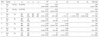
To explore this apparent discrepancy further, we perform linear OLS regressions to predict N_d using SO₄, which is a significant contributor to both marine and continental CCN, and rBC, which should serve as an unambiguous tracer of smoke. Figure 2 shows the results using (a) all variables (AC SO₄, BC SO₄, AC rBC, and BC rBC), (b) only AC and BC SO₄, (c) only AC and BC rBC, (d) only BC SO₄ and rBC, and (e) only AC SO₄ and rBC. The R² for each regression is shown in Fig. 2f and full statistics are provided in Table 1. SO₄ is a better predictor of N_d than rBC alone, although the combination of the two adds predictive power. This result is expected as SO₄ may be contributing to CCN from both “natural” marine (sea spray and oxidation of dimethyl sulfide; see, e.g., Simpson et al., 2014) and “polluted” continental sources (potentially from industrial activity and very likely from biomass burning; see, e.g., Formenti et al., 2003), whereas rBC is only a component of a subset of the continental CCN. The decent correlation of rBC and N_d provides evidence for the influence of smoky continental air on the marine cloud microphysical properties beyond changes in meteorology and marine aerosol sources.

Figure 2 Scatterplot of observed N_d against N_d predicted from a regression using (a) all valid AC SO₄, BC SO₄, AC rBC, and BC rBC observations, (b) only SO₄ observations, (c) only rBC observations, (d) only BC observations, and (e) only AC observations. 31 August and 4 September flights are highlighted in red and blue, respectively. Dashed black lines show the one-to-one line. (f) Bar chart showing R² for all regressions.

Interestingly, the regression using only the BC values of SO₄ and rBC (Fig. 2f; Table 1, row 6) is nearly as skillful as the full regression (Fig. 2f; Table 1, row 3), whereas the regression using only the AC values (Fig. 2f; Table 1, row 7) has comparatively little skill. Moreover, although the coefficients for the regressions including both SO₄ and rBC are not reliable given their mutual correlation (and are provided primarily for the sake of reproducibility), the coefficients of the regressions using only SO₄ (Table 1, row 4) or rBC (Table 1, row 5) also reveal that those regressions are driven by the BC values. This indicates that variability in aerosol properties immediately above the MBL has little immediate impact on the microphysics of the clouds below.

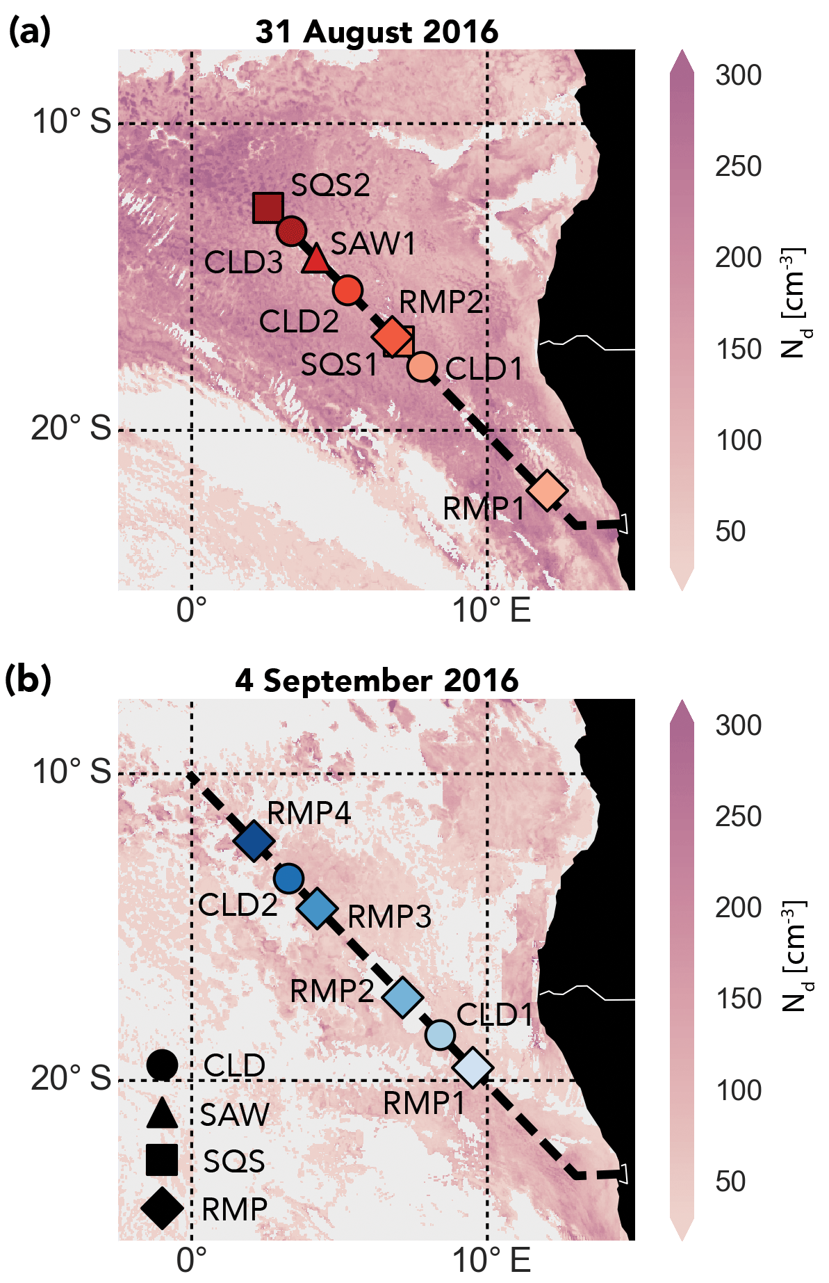
Figure 3 Map of the SEA region with the location of relevant flight legs for the (a) 31 August and (b) 4 September flights shown in shades of red and blue, respectively. The flight track of the P-3 for each day is given by a dashed black line. Background shading is N_d from SEVIRI (12:15 UTC) screened for MBL clouds.

3.2 Case study: comparison of 31 August and 4 September flights

To illustrate the phenomenon of similar above-cloud aerosol profiles leading to different MBL properties, we focus on the two flights highlighted in Fig. 2: 31 August (red) and 4 September (blue). Figure 3 shows the mean location and Table 2 reports the starting and ending latitude, longitude, and time for each flight maneuver analyzed. As can be seen both in Fig. 2 and the SEVIRI N_d imagery in Fig. 3, the 31 August clouds had some of the highest N_d observed in the ORACLES-2016 deployment, whereas the 4 September clouds were on the lower N_d end of the spectrum.

Table 2 Starting and ending latitude, longitude, and time for all the flight legs from the 31 August and 4 September cases used in Figs. 3, 4, and 6.

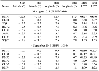
Figure 4 explores each flight maneuver on the two days in more depth, showing (a) vertical profiles (lines) of rBC and cloud-top height (vertical placement of markers) for RMP and SQS legs and (b) the full cloud droplet spectra for CLD and SAW legs. Focusing first on the vertical smoke profiles, rBC concentrations were generally higher just above cloud top on 4 September than they were on 31 August, yet MBL concentrations of rBC were ∼5 times greater on 31 August. Cloud properties (horizontal placement of markers) tell a similar story, with N_d values from 31 August well above those from 4 September. Even within the profiles on 31 August, higher above-cloud rBC values do not necessarily correspond to higher N_d. Particularly high SO₄ values on 31 August (Fig. 2b) likely contributed to the incredibly high N_d of some profiles (e.g., the ∼700 cm⁻³ observed for RMP1) but cannot explain the difference in MBL rBC between the days and thus do not answer the more general question of why the MBL on 31 August was much more polluted than on 4 September.

Figure 4 Cloud microphysical properties and rBC for the 31 August (red) and 4 September (blue) flights. (a) Vertical profiles of rBC number concentration (lines) and average N_d (markers) for each RMP and SQS profile. The vertical positions of the markers indicate cloud-top height for each profile and the horizontal positions indicate the average N_d value. Note that rBC and N_d share the same x axis because they have the same units and similar magnitudes. (b) Average cloud droplet spectra (curves), N_d (ticks on y axis), and r_e (ticks on x axis) for each CLD and SAW leg. Stars indicate the values of N_d and r_e from SEVIRI (SEV) averaged over the 31 August (light red) and 4 September (light blue) flight paths.

There is an approximately 100 m “clear air slot” (Hobbs, 2003), or gap, between the bottom of the aerosol plume and cloud tops for RMP4 on 4 September and a similar drop-off in smoke just above cloud for RMP2, but the RMP1 and RMP3 profiles for that flight show direct instantaneous contact. The narrow gap distance for RMP2 and RMP4 suggests that the 100 m threshold for cloud–aerosol “contact” of Costantino and Bréon (2013) may exclude observations that the 250 and 360 m thresholds of Costantino and Bréon (2010) and Rajapakshe et al. (2017), respectively, would inadvertently include as “mixed” cases.

For the CLD and SAW legs that allowed for more time in cloud, we show the averaged cloud droplet spectra (curves) along with average N_d and r_e (ticks) in Fig. 4b. CLD1 and CLD2 follow RMP1 and RMP3, respectively, on 4 September (Fig. 3), with above-cloud legs with some cloud “dips” immediately preceding the CLD legs, suggesting similar direct instantaneous smoke–cloud contact for those legs. Again, the 31 August flight shows much clearer evidence of MBL pollution, with droplet spectra shifted toward smaller drop sizes and higher concentrations, and thus higher N_d and lower r_e, compared with the 4 September values. This result is consistent with the SEVIRI N_d values (stars), although SEVIRI N_d is systematically lower than the in situ values for both days. The presence of overlying aerosol can create a low bias in remotely sensed COT without having a large effect on remotely sensed r_e (Haywood et al., 2004; Wilcox et al., 2009), leading to an expected low bias in N_d.

Whereas the vertical profiles of BBA in Fig. 4a look fairly comparable, the WRF–AAM curtains along the HYSPLIT back trajectories shown in Fig. 5 reveal considerable variation in the histories of smoke–cloud contact between the two cases. The 250 m trajectories both originate in the Southern Ocean 5 days before sampling but differ markedly in the smoke environments they encountered before being sampled, as shown in the curtain plots of WRF–AAM biomass burning CO concentrations for 31 August in Fig. 5b and 4 September in Fig. 5c. The MBL sampled on 31 August appears to have been in contact with smoke for several days beforehand, whereas the MBL on 4 September was overlain with clean air until ∼1.5 days before sampling. Given the sharp gradient at the lower boundary of the smoke plume seen in both the observations and the model output, direct contact may have been even more limited. Observed CO (Fig. 6) is qualitatively consistent with the WRF–AAM output, with MBL average CO values on 31 August considerably above those from 4 September and among the highest seen during the deployment (all other flights shown in thin grey lines).

Figure 5 (a) Map of HYSPLIT MBL back trajectories for 31 August (red) and 4 September (blue). Circles are plotted every 24 h after initialization. The ORACLES-2016 routine flight path is plotted as a dashed black line for reference. Curtains of WRF–AAM biomass-burning-tagged CO along the path of the trajectories are plotted in (b) for 31 August and (c) for 4 September, with the trajectory altitude indicated by the dashed black line.

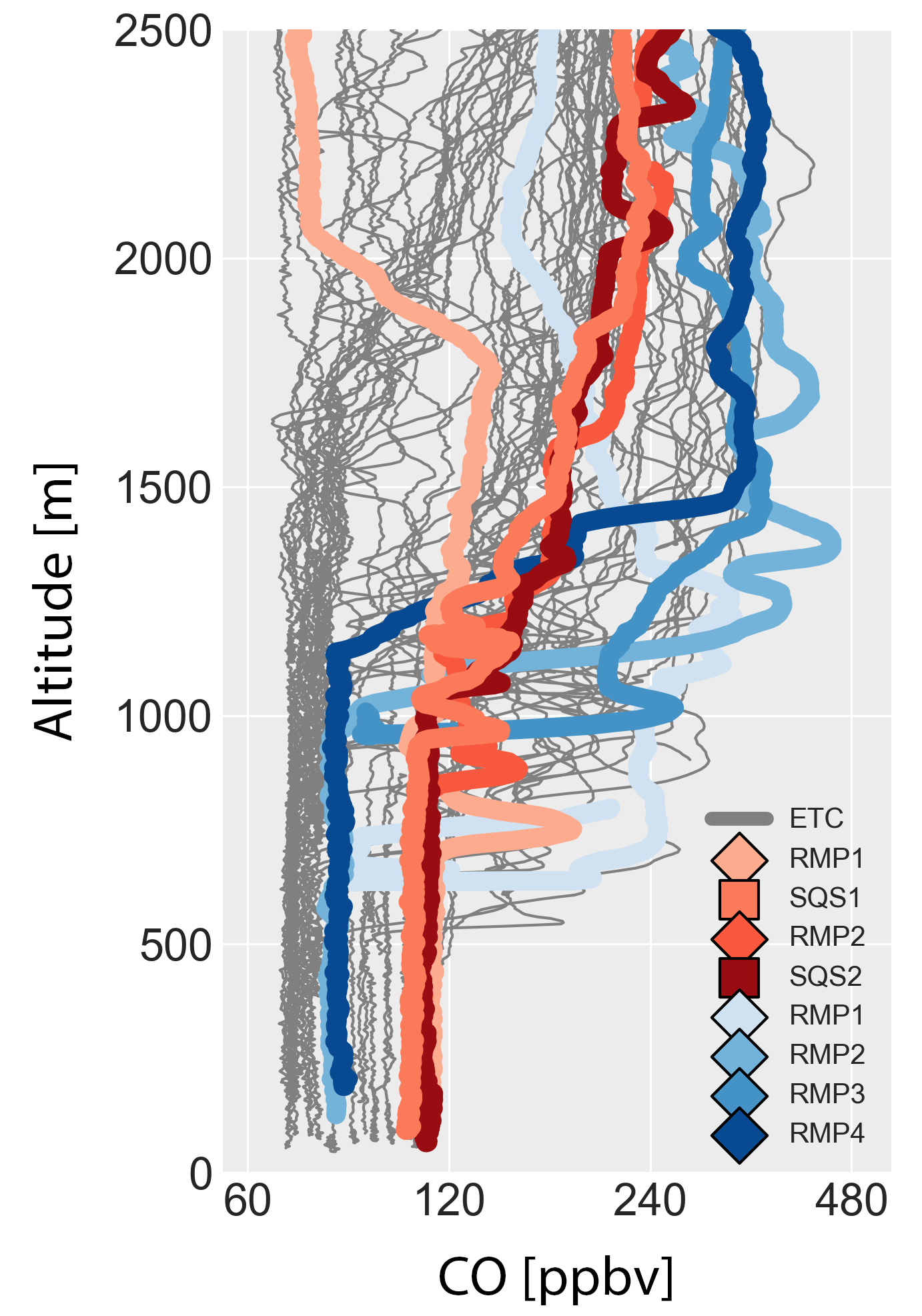
Figure 6 Vertical profiles of observed CO for all ORACLES-2016 flights (grey lines), with the profiles from 31 August and 4 September highlighted in shades of red and blue, respectively.

4 Discussion

4.1 Timescales for the entrainment of free tropospheric CCN

The importance of the different entrainment histories of the 31 August and 4 September cases, and the implications for the SEA region more generally, can be illuminated using an idealized framework. Assuming no other source or sink terms besides FT entrainment and that entrainment is in approximate balance with large-scale subsidence, the rate of increase in MBL CCN concentrations, CCN_MBL, for a constant exposure to a directly-above-cloud FT CCN concentration, CCN_FT, can be expressed as

$$\begin{array}{}\text{(6)}& {\displaystyle \frac{\partial {\text{CCN}}_{\text{MBL}}}{\partial t}}={\displaystyle \frac{w_{\text{e}}}{z_i}}({\text{CCN}}_{\text{FT}}-{\text{CCN}}_{\text{MBL}}),\end{array}$$

where w_e is the entrainment rate, z_i is the height of the MBL, and t is time (Wood et al., 2012). This equation has a characteristic e-folding timescale (τ_ent) for CCN_MBL to equilibrate with CCN_FT:

$$\begin{array}{}\text{(7)}& {\mathit{\tau }}_{\mathrm{ent}}={\displaystyle \frac{z_i}{w_{\mathrm{e}}}}.\end{array}$$

For a typical entrainment rate of 0.4 cm s⁻¹ (Faloona et al., 2005; Wood and Bretherton, 2004) and MBL height of 1 km, the characteristic timescale is ∼3 days for the CCN concentration in the MBL to reach equilibrium with FT levels. This estimate is in line with previous values of, e.g., ∼4 days for the northeast Atlantic (Bretherton et al., 1995) and ∼3 days for the tropical Pacific (Simpson et al., 2014). Figure 7a shows that for a plausible range of w_e from 0.2–0.7 cm s⁻¹ (Faloona et al., 2005) and z_i from 500–1500 m, the characteristic e-folding timescale for entrainment mixing of MBL and FT air varies from approximately 1 day to 1 week.

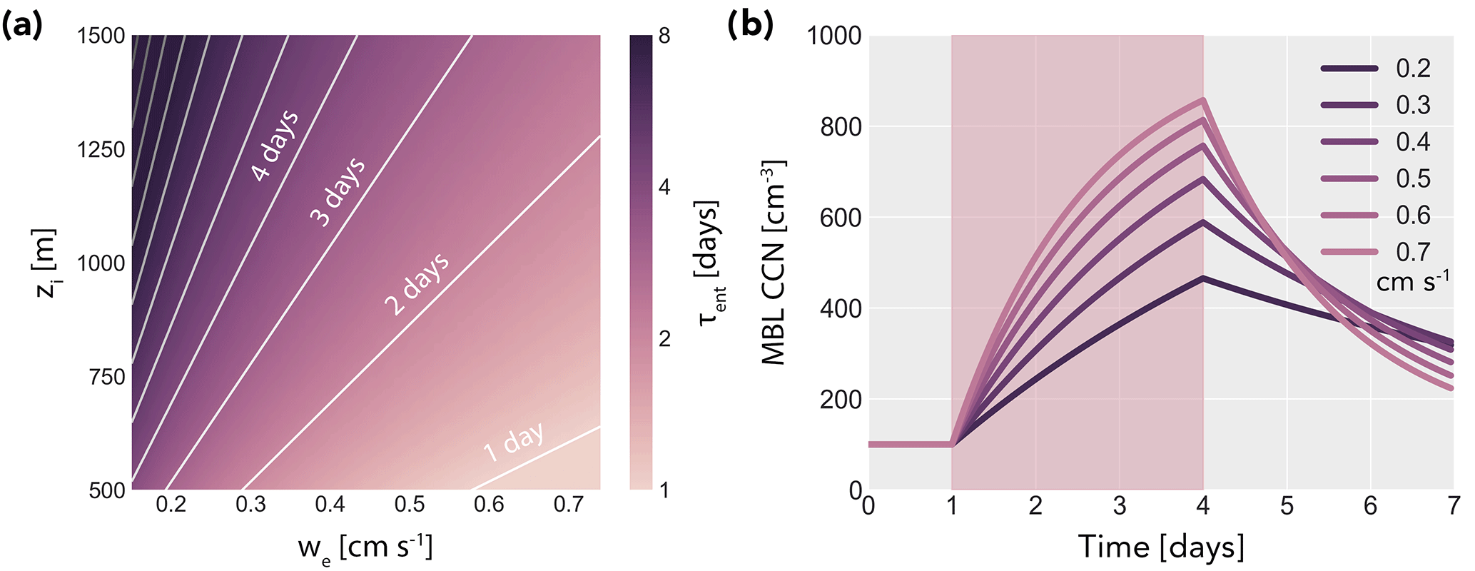
Figure 7 (a) Characteristic (e-folding) entrainment mixing timescale for a range of plausible z_i and w_e values. Contours at 1-day intervals for reference. (b) Evolution of CCN_MBL over time in response to the introduction of a smoke plume with CCN_FT=1000 cm⁻³ at day 1 and its removal at day 4 (highlighted). Curves show results for a range of entrainment timescales with z_i=1 km and w_e varying between 0.2 and 0.7 cm s⁻¹.

To illustrate the effects of both differing entrainment mixing timescales and sampling at different times along the MBL evolution, we conduct a thought experiment in which an MBL in equilibrium with a “clean” FT with CCN_FT=100 cm⁻³ is exposed to smoky FT air with CCN_FT=1000 cm⁻³ for 3 days, after which “clean” FT conditions return. Figure 7b shows the results of this scenario with an MBL with z_i=1 km and a range of w_e values. Three main features stand out: (1) for any given entrainment timescale, the strength of the aerosol–cloud interactions estimated from a single snapshot during smoke contact will depend heavily on the time of observation; (2) for any given point in time, the entrainment rate can cause up to a factor of 2 difference in CCN_MBL; and (3) for all but the most rapidly entraining cases, MBLs remain more polluted 24 h after exposure to smoke than they were after the first 24 h of smoke exposure.

4.2 Effects of precipitation

The real situation in the SEA is more complicated than the equations presented here because it is unrealistic to expect CCN_FT to remain constant over both long time periods and large spatial gradients, and precipitation–coalescence scavenging acts as a sink for CCN that is unaccounted for above, among other issues. Precipitation, in particular, has been shown to be a primary driver of regional and seasonal N_d variability in subtropical Sc decks (Mohrmann et al., 2017; Wood et al., 2012) and even moderate amounts of drizzle can rapidly deplete an MBL of CCN (Wood, 2006).

To assess how the inclusion of precipitation processes affects the discussion of entrainment above, we adapt a fuller Lagrangian MBL CCN budget equation from Wood et al. (2012) and Mohrmann et al. (2017):

$$\begin{array}{ll}{\displaystyle \frac{\text{D}}{\text{D}t}}& {\displaystyle }{\text{CCN}}_{\text{MBL}}={\dot{\text{CCN}}}_{\text{FT}}+{\dot{\text{CCN}}}_{\text{SS}}+{\dot{\text{CCN}}}_{\text{Growth}}\\ \text{(8)}& {\displaystyle }& {\displaystyle }+{\dot{\text{CCN}}}_{\text{Precip}}+{\dot{\text{CCN}}}_{\text{Dry}},\end{array}$$

where the subscript FT refers to the entrainment of air from the free troposphere (Eq. 6), SS to sea spray, “Growth” to growth in the MBL from secondarily produced and other small particles to CCN active sizes, “Precip” to precipitation–coalescence scavenging, and “Dry” to dry deposition. As in Wood et al. (2012) and Mohrmann et al. (2017), we eliminate the growth and dry deposition terms because of their uncertain formulations and negligible contributions to the total CCN budget.

Following Wood (2006), the loss of CCN due to coalescence scavenging is given by

$$\begin{array}{}\text{(9)}& {\dot{\text{CCN}}}_{\text{Precip}}=-{\displaystyle \frac{K{P}_{\text{CB}}h}{z_i}}{N}_{\text{d}},\end{array}$$

where K (= 2.25 m² kg⁻¹) is a constant that depends on the collection efficiency of drizzle drops, P_CB is the precipitation rate at cloud base, and h is the cloud thickness. This formulation assumes that the accretion of cloud droplets onto drizzle drops (coalescence) is the primary sink of CCN rather than nonactivated MBL CCN being washed out by falling rain, which is true for the lightly drizzling Sc decks. Even if the drizzle does not reach the ocean surface, CCN are lost because thousands of cloud drops can be collected together and evaporate in the MBL to form one larger haze particle, conserving mass but depleting aerosol number. For an appropriate supersaturation, we can assume N_d and CCN_MBL are approximately equal.

To complete our CCN budget equation, we account for sea spray as

$$\begin{array}{}\text{(10)}& {\dot{\text{CCN}}}_{\text{SS}}={\displaystyle \frac{F\left(\mathit{\sigma }\right)U_{\mathrm{10}}^{\mathrm{3.41}}}{z_i}},\end{array}$$

where F(σ) is a function of supersaturation and U₁₀ is wind speed at 10 m (Clarke et al., 2006; Wood et al., 2012). We assume a supersaturation of 0.3 %, corresponding to F(σ)=214 m⁻³ (m s${}^{-\mathrm{1}}{)}^{-\mathrm{2.41}}$, and a mean wind speed of 7 m s⁻¹, which is representative of the SEA.

We can now write the full Lagrangian CCN budget equation as

$$\begin{array}{}\text{(11)}& {\displaystyle }& {\displaystyle \frac{\text{D}}{\text{D}t}}{\text{CCN}}_{\text{MBL}}={\displaystyle \frac{w_{\text{e}}+K{P}_{\text{CB}}h}{z_i}}({\text{CCN}}_{\text{eq}}-{\text{CCN}}_{\text{MBL}}),\text{(12)}& {\displaystyle }& {\displaystyle }{\text{CCN}}_{\text{eq}}={\displaystyle \frac{{\text{CCN}}_{\text{FT}}+\frac{F\left(\mathit{\sigma }\right)U_{\mathrm{10}}^{\mathrm{3.41}}}{w_{\text{e}}}}{\mathrm{1}+\frac{K{P}_{\text{CB}}h}{w_{\text{e}}}}}.\end{array}$$

Note that CCN_eq, which accounts for the sea spray source and the precipitation sink in addition to FT entrainment, has taken the place of CCN_FT from earlier.

By adding precipitation, the equilibration timescale is reduced as the timescales for FT entrainment and coalescence scavenging add in parallel:

$$\begin{array}{}\text{(13)}& \mathit{\tau }={\left({\displaystyle \frac{\mathrm{1}}{{\mathit{\tau }}_{\text{ent}}}}+{\displaystyle \frac{\mathrm{1}}{{\mathit{\tau }}_{\text{Precip}}}}\right)}^{-\mathrm{1}}={\displaystyle \frac{z_i}{w_{\text{e}}+K{P}_{\text{CB}}h}}.\end{array}$$

Figure 8a shows the full equilibration timescale for the same range of w_e as earlier and a range of P_CB from 0–1 mm day⁻¹, assuming z_i=1 km and h=300 m. Although the timescale is reduced with increasing drizzle, the magnitude remains on the order of days for the precipitation values experienced in the Sc decks.

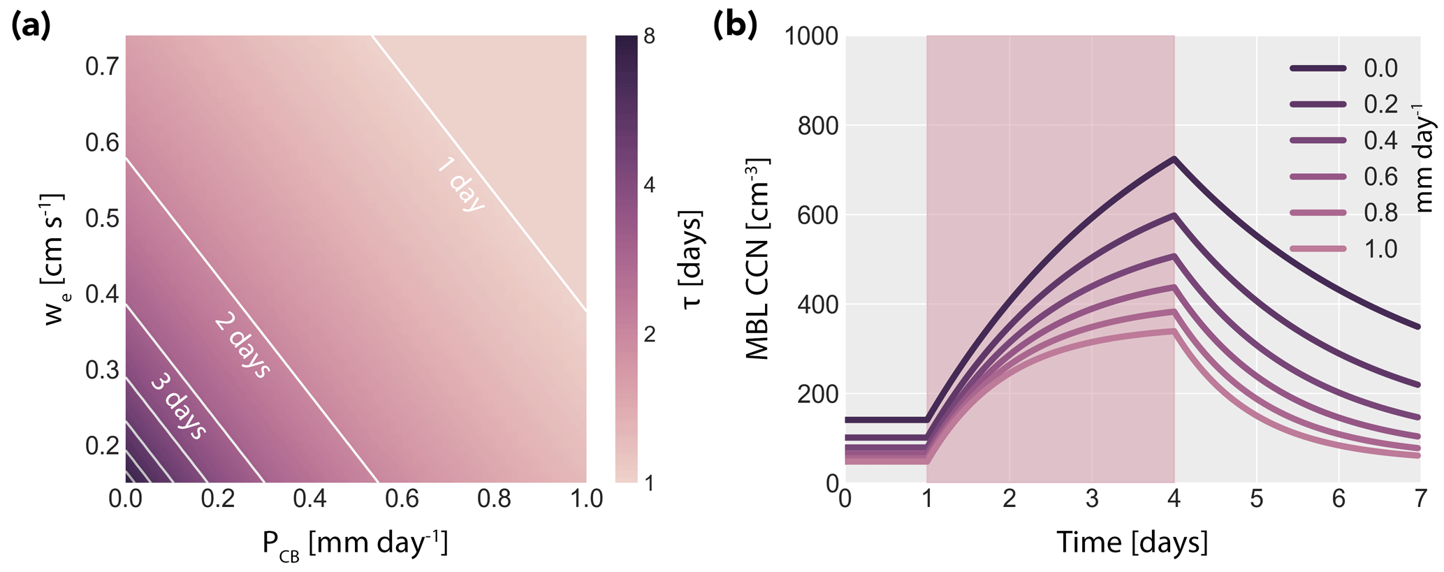
Figure 8 (a) Characteristic (e-folding) entrainment mixing timescale for a range of plausible w_e and P_CB values. Contours at 1-day intervals for reference. (b) Evolution of CCN_MBL over time in response to the introduction of a smoke plume with CCN_FT=1000 cm⁻³ at day 1 and its removal at day 4 (highlighted). Curves show results for a range of equilibration timescales with z_i=1 km, w_e=0.4 cm s⁻¹, h=300 m, and P_CB varying between 0 and 1 mm day⁻¹.

Figure 8b shows the full CCN budget equation applied to a case with CCN_FT=1000 cm⁻³, w_e=0.4 cm s⁻¹, z_i=1 km, h=300 m, and a range of P_CB values. Unsurprisingly, as precipitation increases, the equilibrium level of CCN_MBL is reduced regardless of how much smoke is present. However, the key features are qualitatively the same as in Fig. 7b: (1) for any given precipitation rate, the strength of the estimated aerosol–cloud interactions will depend heavily on the time of observation; (2) for any given point in time, the precipitation rate can cause substantial differences in CCN_MBL; and (3) for light drizzle, MBLs remain more polluted 24 h after exposure to smoke than they were after the first 24 h of smoke exposure.

Heavy drizzle was not observed on the 4 September flight, but instantaneous daytime precipitation measurements would not be sufficient as an indication of coalescence scavenging in any case given that Sc drizzle tends to peak overnight (Smalley and L'Ecuyer, 2015). Additionally, the association of high (low) precipitation with low (high) N_d suffers from ambiguous causality: the different precipitation rates may drive the N_d values, but alternatively the N_d values may drive the frequency and intensity of precipitation (i.e., precipitation suppression and/or lifetime effects). Without any additional information, it would be difficult to distinguish between the potential roles of precipitation versus entrainment history in explaining the vastly different MBL aerosol and cloud properties observed between 31 August and 4 September. Fortunately, for the ORACLES-2016 flights CO measurements can be invoked to resolve this ambiguity. Coalescence scavenging may have been the preferred explanation for the differences between 31 August and 4 September had the two days seen similar levels of MBL CO, which is not removed by precipitation processes. However, because MBL CO was much higher on 31 August than on 4 September (Fig. 6), the difference in smoke entrainment history is the most plausible cause of the differences in MBL aerosol loading and N_d.

5 Summary and conclusions

Data from the September 2016 deployment of the ORACLES campaign show that the presence of smoke from biomass burning in southern Africa in the MBL is associated with cloud microphysical changes, but the presence of smoke near cloud top has little association by itself with the cloud properties below. This finding is illustrated by two flights that have similar vertical distributions of above-cloud BBA but markedly different MBL pollution levels. Model results suggest that the MBL air sampled on 31 August had been in contact with smoke for a considerably longer time period than that sampled on 4 September. We argue that considering the prior history of the smoke and MBL air is key to understanding the large variations between cases with similar vertical profiles in the FT.

A serious treatment of the time dependence of the entrainment process has a number of implications for studies that use a more instantaneous, or “Eulerian”, viewpoint, such as the A-train studies reviewed above. For instance, because the climatological MBL flow is southerly in the SEA, an instantaneous snapshot of smoke–cloud contact in the southern reaches of the domain may underestimate the microphysical effects by not accounting for their manifestation as the clouds and MBL smoke advect northward. Similarly, apparently “clean” cases in the northern part of the domain may have been polluted further south, complicating efforts to compare “mixed” and “unmixed” statistics.

Recent modeling work suggests that accurately characterizing RF_ACI is important for both regional and global estimates of radiative forcing: Lu et al. (2018) find that smoke over the SEA can produce a net −7 to −8 W m⁻² forcing, primarily due to the Twomey effect, which corresponds approximately to an appreciable −0.089 W m⁻² forcing globally during the biomass burning season. Previous LES modeling of the Sc to cumulus transition also suggested that aerosol–cloud interactions over the SEA could contribute to net negative radiative forcings (Yamaguchi et al., 2015; Zhou et al., 2017). Inaccurate observational estimates of the magnitude of aerosol–cloud interactions over the SEA can thus greatly hinder our understanding of the magnitude and sign of the net radiative forcing of smoke over the SEA and how changes in southern African biomass burning may affect regional and global climate. Although fire activity in southern Africa has been increasing over the past decade in opposition to global trends of reduced burned area associated with anthropogenic land-use change (Andela et al., 2017), it is reasonable to expect that biomass burning may decrease in the future in response to concerns about the negative population health consequences of particulate matter due to fires (Johnston et al., 2012) and the possibility that smoke has been suppressing precipitation on the continent (Hodnebrog et al., 2016). Therefore, an accurate estimate of the climatic effects from a changing BBA loading over the SEA is highly societally relevant.

Future work is needed to assess to what extent a Lagrangian framework (Eastman and Wood, 2016; Mauger and Norris, 2010) accounting for the transport history of both the smoke and clouds differs from the traditional Eulerian framework in terms of estimated aerosol–cloud interactions. Of course, other sources and sinks of aerosols besides FT entrainment – e.g., precipitation – act on similar timescales and may be better understood in a Lagrangian framework as well. Combining observations with the history of air masses from models is likely necessary to understand MBL aerosol loading and thus RF_ACI and the resulting cloud adjustments.