the Creative Commons Attribution 4.0 License.
the Creative Commons Attribution 4.0 License.
 | 31 Aug 2018
Experimental and model estimates of the contributions from biogenic monoterpenes and sesquiterpenes to secondary organic aerosol in the southeastern United States
Havala O. T. Pye
Jia He
Yunle Chen
Benjamin N. Murphy
Atmospheric organic aerosol (OA) has important impacts on climate and human health but its sources remain poorly understood. Biogenic monoterpenes and sesquiterpenes are important precursors of secondary organic aerosol (SOA), but the amounts and pathways of SOA generation from these precursors are not well constrained by observations. We propose that the less-oxidized oxygenated organic aerosol (LO-OOA) factor resolved from positive matrix factorization (PMF) analysis on aerosol mass spectrometry (AMS) data can be used as a surrogate for fresh SOA from monoterpenes and sesquiterpenes in the southeastern US. This hypothesis is supported by multiple lines of evidence, including lab-in-the-field perturbation experiments, extensive ambient ground-level measurements, and state-of-the-art modeling. We performed lab-in-the-field experiments in which the ambient air is perturbed by the injection of selected monoterpenes and sesquiterpenes, and the subsequent SOA formation is investigated. PMF analysis on the perturbation experiments provides an objective link between LO-OOA and fresh SOA from monoterpenes and sesquiterpenes as well as insights into the sources of other OA factors. Further, we use an upgraded atmospheric model and show that modeled SOA concentrations from monoterpenes and sesquiterpenes could reproduce both the magnitude and diurnal variation of LO-OOA at multiple sites in the southeastern US, building confidence in our hypothesis. We estimate the annual average concentration of SOA from monoterpenes and sesquiterpenes in the southeastern US to be roughly 2 µg m−3.
- Article
(2474 KB) - Full-text XML
-
Supplement
(2301 KB) - BibTeX
- EndNote


Organic aerosol (OA) constitutes a substantial fraction of ambient fine particulate matter (PM) and has large impacts on air quality, climate change, and human health (Carslaw et al., 2013; Lelieveld et al., 2015). OA can be directly emitted from sources (primary OA, POA) or formed by the oxidation of volatile organic compounds (VOCs) (secondary OA, SOA). Global measurements revealed the dominance of SOA over POA in various atmospheric environments (Jimenez et al., 2009; Ng et al., 2010). VOCs can be emitted from natural sources (i.e., biogenic) or human activities (i.e., anthropogenic). However, the relative contribution of biogenic and anthropogenic sources to SOA formation in the atmosphere is poorly constrained. This knowledge is critical for formulating effective pollution control strategies that aim at reducing ambient PM concentrations and accurately assessing the climate effects of OA (Hallquist et al., 2009). Biogenic VOCs such as monoterpenes (MT, C10H16) and sesquiterpenes (SQT, C15H24) are recognized as critical precursors of SOA (Tsigaridis et al., 2014; Hodzic et al., 2016; Pye et al., 2010). The predicted global SOA production from MT and SQT varies from 14 to 246 Tg yr−1 (Spracklen et al., 2011; Pye et al., 2010). This large variation in model estimates arises from a number of factors (including uncertainty in SOA yield) and introduces significant uncertainties in estimating OA concentrations and its subsequent influences on climate and human exposure.
The large model uncertainties call for ambient observations to constrain model results. Isolating and measuring SOA production from specific sources are challenging because SOA is a complex mixture consisting of thousands of compounds and SOA evolves dynamically in the atmosphere. A widely used method to apportion OA into different characteristic sources is positive matrix factorization (PMF) analysis on the organic mass spectra measured by aerosol mass spectrometer (AMS) (Ulbrich et al., 2009; Jimenez et al., 2009; Ng et al., 2010). PMF–AMS analysis groups OA constituents with similar mass spectra and temporal variations into characteristic OA subtypes (i.e., factors). This analysis has revealed that the concentration of oxygenated OA (OOA), which is a surrogate of SOA, is much greater than that of hydrocarbon-like OA (HOA), which is a surrogate of POA (Zhang et al., 2007). In many circumstances, especially in warmer months, more than one SOA factor is resolved from PMF analysis, often including less-oxidized oxygenated OA (LO-OOA, also denoted as semi-volatile oxygenated organic aerosol in older studies) and more-oxidized oxygenated OA (MO-OOA, also denoted as low-volatility oxygenated organic aerosol in older studies). LO-OOA and MO-OOA are differentiated by their degree of carbon oxidation. These two factors together account for more than half of total submicron OA (Crippa et al., 2014; Xu et al., 2015a; Jimenez et al., 2009). Despite their large abundance, the sources of LO-OOA and MO-OOA are unclear and likely vary with location and season. Early studies proposed that LO-OOA is freshly formed SOA from various sources and evolves into MO-OOA with photochemical aging in the atmosphere (Jimenez et al., 2009; Ng et al., 2010). Later, a number of possible sources have been proposed for MO-OOA, including SOA from long-range transport (Hayes et al., 2013; Robinson et al., 2011b), aged biomass burning OA (Bougiatioti et al., 2014; Grieshop et al., 2009), humic-like substances (El Haddad et al., 2013), highly oxygenated molecules (HOMs) formed in the oxidation of monoterpenes (Mutzel et al., 2015; Ehn et al., 2014), and aqueous-phase processing (W. Xu et al., 2017). Regarding the sources of LO-OOA, Zotter et al. (2014) applied radiocarbon analysis and showed that 68 %–75 % of carbon in LO-OOA in California stems from fossil sources. In the southeastern US, Xu et al. (2015a) suggested that the oxidation of biogenic β-pinene by nitrate radicals (NO3) contributes to LO-OOA, though this reaction alone cannot replicate the magnitude of LO-OOA (Pye et al., 2015).
Many different sources of LO-OOA and MO-OOA have been proposed primarily based on comparing the mass spectra between ambient OA factors and laboratory-generated SOA (Jimenez et al., 2009; Kiendler-Scharr et al., 2009; Ng et al., 2010). While the mass spectra comparison approach largely improves our understanding of ambient OA factors, this approach has the following limitations. Firstly, the similarity between two mass spectra is a subjective determination. In other words, a good correlation coefficient (R) value between the mass spectra of an ambient OA factor and a specific type of laboratory SOA does not imply that the laboratory SOA contributes to the specific ambient OA factor. Secondly, such subjectively defined similarity does not provide quantitative insights into the contribution of SOA from a certain source to a specific OA factor. For example, previous studies have shown that the mass spectrum of laboratory α-pinene SOA is the most similar to that of LO-OOA (Jimenez et al., 2009; Kiendler-Scharr et al., 2009; Ng et al., 2010). However, this similarity neither guarantees that α-pinene SOA is exclusively apportioned into LO-OOA, nor provides information regarding what fraction of α-pinene SOA is apportioned into LO-OOA in ambient environments. Thus, uncertainties associated with the sources of these OA factors still exist. Considering the large abundance of OOA subtypes and their use as surrogates for ambient SOA, understanding the sources of the compounds composing these two OOA subtypes is critical to constrain atmospheric models and the SOA budget.
In this study, we integrate lab-in-the-field experiments, extensive ambient ground-level measurements, and state-of-the-art modeling to improve the understanding of the sources of OA factors and better constrain the OA budget from MT and SQT. Based on lab-in-the-field experiments, we provide objective evidence that newly formed SOA from α-pinene (an important monoterpene) and β-caryophyllene (an important sesquiterpene) is dominantly apportioned to LO-OOA in the southeastern US. In addition, we model the SOA concentration from the oxidation of MT and SQT (denoted as SOAMT+SQT) and show that SOAMT+SQT reasonably reproduces the magnitude and diurnal variability of LO-OOA measured at multiple sites in the southeastern US. Together with other evidence in the literature, we propose that LO-OOA can be used as a measure of SOAMT+SQT in the southeastern US. Finally, we discuss how the lab-in-the-field approach allows for the study of SOA formation under realistic atmospheric conditions, which bridges laboratory studies and field measurements and provides a direct way to evaluate the atmospheric relevancy of laboratory studies.
2.1 Lab-in-the-field perturbation experiments
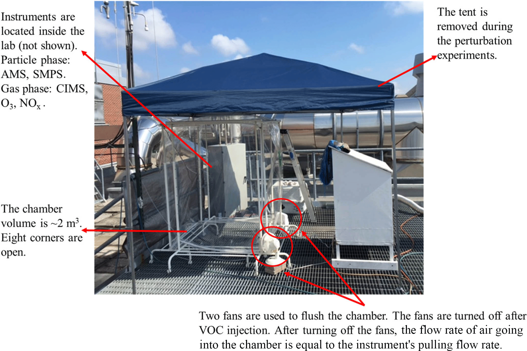
The perturbation experiments were performed in July–August 2016 on the rooftop of the Environmental Science and Technology building on the Georgia Institute of Technology campus. This measurement site is an urban site in Atlanta, Georgia. Multiple ambient field studies have been performed at this site previously (Xu et al., 2015b; Hennigan et al., 2009; Verma et al., 2014). A roughly 2 m3 Teflon chamber (cubic shape) (Fig. 1) was placed outdoors on the rooftop of the building. The eight corners of the chamber were open () to the atmosphere to allow for continuous exchange of air with the atmosphere. The perturbation procedure is briefly described below and illustrated in Fig. A1. Firstly, we continuously flushed the chamber with ambient air using two fans, which were placed at two corners of the chamber. During this flushing period, all instruments sampled ambient air and were not connected to the chamber. The flushing period lasted at least 3 h to ensure that the air composition in the chamber is the same as the ambient composition. Secondly, we stopped both fans and connected all instruments to the chamber. Because of the continued sampling by the instruments (∼20 L min−1) and the open corners of the chamber, ambient air continuously entered the chamber, even though the two fans were turned off. Thirdly, after sampling the chamber for about 30 min, we injected a known amount of VOC (liquid) into the chamber with a needle, and the liquid vaporized upon injection. We continuously monitored the chamber composition for ∼40 min after VOC injection. Lastly, we disconnected all instruments from the chamber, sampled ambient air, and turned on two fans to flush the chamber to prepare for the next perturbation experiment.
Each perturbation experiment can be divided into the following four periods: Amb_Bf (30 min ambient measurement period before sampling chamber), Chamber_Bf (from sampling chamber to VOC injection, a period ∼30 min), Chamber_Af (from VOC injection to stopping the sampling of chamber, a period ∼40 min), and Amb_Af (30 min ambient measurement period after sampling chamber). We perform PMF analysis on the combined ambient and perturbation data and then calculate the changes in the mass concentration of OA factors based on the difference between Chamber_Bf and Chamber_Af, after taking ambient variations into account. The detailed procedure is presented in Appendix A. We develop a comprehensive set of criteria to determine if the changes are statistically significant and if the changes are simply due to ambient variations. The details of these criteria are also discussed in Appendix A.
We perturbed the chamber content by injecting one of the following VOCs: isoprene, α-pinene, β-caryophyllene, m-xylene, or naphthalene, which are major biogenic or anthropogenic emissions. We focused on α-pinene and β-caryophyllene because of their large abundances in their classes and the fact that they are widely studied in the literature (Eddingsaas et al., 2012a; Kurtén et al., 2015; Tasoglou and Pandis, 2015; Ehn et al., 2014; Pathak et al., 2007). For example, α-pinene accounts for about half of monoterpene emissions (Guenther et al., 2012) and β-caryophyllene is one of the most abundant sesquiterpenes (Helmig et al., 2007). We aim to inject as low of a VOC mixing ratio as possible to be atmospherically relevant. If the injection amount is too large, too much SOA will be produced, which will bias subsequent analysis. We use a needle to inject liquid sample into the chamber. Limited by the needle size, 0.2 µL is selected because it is the minimal amount we could inject with reliable accuracy. The VOC oxidation occurred in ambient air (inside the chamber) and lasted ∼40 min. The OA concentration in the chamber after perturbation ranges from 4 to 16 µg m−3, which is within the range of typical ambient OA concentrations in the southeastern US.
We note that several previous studies have used ambient air (Palm et al., 2018; Leungsakul et al., 2005; Peng et al., 2016), but the experimental approaches and purposes of previous studies are different from this study. For example, in Leungsakul et al. (2005), rural ambient air was used to flush and clean the 270 m3 outdoor chamber reactor. After the flushing, both VOCs and oxidants were injected to produce SOA, the concentrations of which were orders of magnitude higher than atmospheric levels. In this study, we use ambient air with preexisting OA in order to examine which factor(s) the fresh SOA from injected VOC are apportioned into by PMF analysis. We aim to produce SOA only from injected VOC, so an important distinction between our study and previous work is that we perturbed the ambient air by only VOCs and no additional oxidants were introduced into the chamber.
The perturbation experiments are designed to address some limitations of the mass spectra comparison approach by providing objective and quantitative evaluations. By producing SOA from a known precursor, PMF analysis allows for the apportionment of the newly formed SOA into various factors without any subjective judgement on the similarity in mass spectra and provides quantification of the fraction of the newly formed SOA that is apportioned into each factor. The perturbation experiments utilize the actual mixing between ambient OA and newly formed SOA from perturbation, which a standard chamber experiment would not achieve, meaning that the performance of the factorization can be more directly inspected. In addition, as the same instrument setup is used for both ambient sampling and perturbation experiments, factorization results are free of instrument tuning issues.
2.2 Analytical instruments
A suite of analytical instruments was deployed to characterize both the gas-phase and particle-phase compositions. The particle-phase composition was monitored by a scanning mobility particle sizer (SMPS, TSI) and a high-resolution time-of-flight aerosol mass spectrometer (HR-ToF-AMS, Aerodyne), which shared the same stainless steel sampling line. A diaphragm pump (flow rate ∼8 L min−1) was connected to this sampling line, which increased the sampling flow rate and reduced particle loss in the sampling line by reducing the residence time in the tubing. The HR-ToF-AMS measures the chemical composition and size distribution of submicron non-refractory species (NR-PM1) with high temporal resolution. The instrument details about HR-ToF-AMS have been extensively discussed in the literature (Canagaratna et al., 2007; DeCarlo et al., 2006) and the operation of HR-ToF-AMS in this study is described in Sect. S2 of the Supplement.
The gas-phase composition and oxidation products were monitored by an O3 analyzer (Teledyne T400, lower detectable limit 0.6 ppb), an ultrasensitive chemiluminescence NOx monitor (Teledyne 200EU, lower detectable limit 50ppt), and a high-resolution time-of-flight chemical ionization mass spectrometer (HR-ToF-CIMS). The HR-ToF-CIMS with I− as the regent ion can measure a suite of oxygenated volatile organic compounds (oVOCs) at high frequency (1 Hz). The detailed working principles and sampling protocol can be found in Lee et al. (2014). The concentrations of VOCs were not measured in this study. All gas-phase measurement instruments shared the same Teflon sampling line. Similar to the particle sampling line, a diaphragm pump (flow rate ∼8 L min−1) was connected to the gas sampling line to reduce the residence time in the tubing.
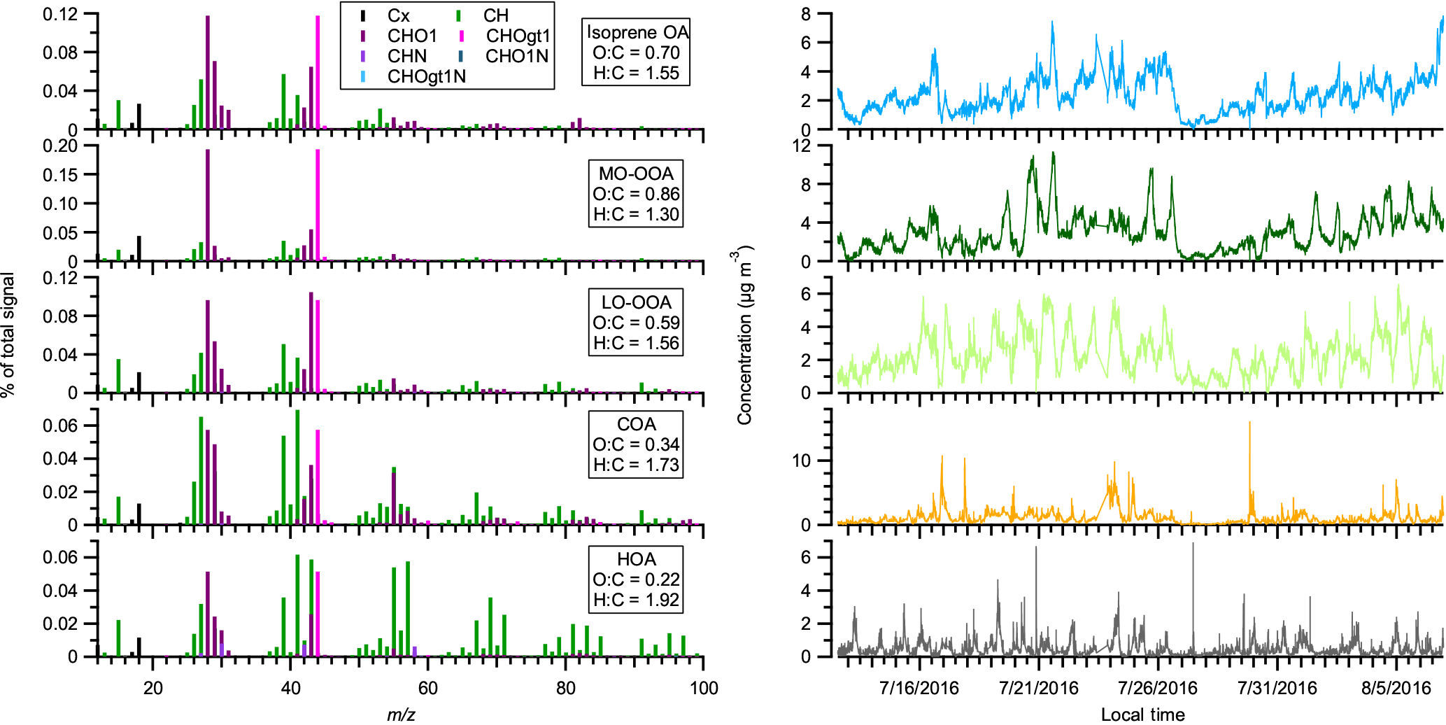
Figure 2The mass spectra and time series of OA factors in the perturbation study. The time series includes both the ambient data and perturbation experiment data.
2.3 Positive matrix factorization (PMF) analysis
PMF analysis has been widely used for aerosol source apportionment in the atmospheric chemistry community (Jimenez et al., 2009; Crippa et al., 2014; Xu et al., 2015a; Ng et al., 2010; Ulbrich et al., 2009; Beddows et al., 2015; Visser et al., 2015). PMF solves the bilinear unmixing factor model by minimizing the summed least squares errors of the fit weight ed with the error estimates of each measurement (Paatero and Tapper, 1994; Ulbrich et al., 2009). We utilized the PMF2 solver, which does not require a priori information and reduces subjectivity. In this study, we performed PMF analysis on the high-resolution mass spectra of organic aerosol (inorganic species are excluded) of combined ambient and perturbation data in the 1-month measurements. Considering that (1) the perturbation data only account for ∼10 % of total data and (2) the OA concentration is similar between the perturbation experiments and typical ambient measurements, the perturbation experiments do not create a new factor that does not already exist in the ambient data. This is desirable because it allows PMF analysis to apportion the newly formed OA in the perturbation experiments into preexisting OA factors in the atmosphere.
We resolved five OA factors, including hydrocarbon-like OA (HOA), cooking OA (COA), isoprene-derived OA (isoprene OA), less-oxidized oxygenated OA (LO-OOA), and more-oxidized oxygenated OA (MO-OOA). The time series and mass spectra of OA factors are shown in Fig. 2. The same five factors have been identified at the same measurement site and extensively discussed in the literature (L. Xu et al., 2015a, b, 2017). Below, we only provide a brief description of these OA factors and more details are discussed in Sect. S3 of the Supplement. The mass spectrum of HOA is dominated by hydrocarbon-like ions ( ions) and HOA is a surrogate of primary OA from vehicle emissions (Zhang et al., 2011). For COA, its concentration is higher at mealtimes and its mass spectrum is characterized by a prominent signal at ions (m∕z 41) and (m∕z 55), which likely arise from fatty acids (Huang et al., 2010; Mohr et al., 2009; Allan et al., 2010). The mass spectrum of isoprene OA is characterized by a prominent signal at ions (m∕z 53) and C5H6O+ (m∕z 82) and is related to the reactive uptake of isoprene oxidation products, isoprene epoxydiols (IEPOX) (Budisulistiorini et al., 2013; Hu et al., 2015; Robinson et al., 2011a; Xu et al., 2015a). LO-OOA and MO-OOA are named based on their differing carbon oxidation state: from −0.70 to −0.34 for LO-OOA and from −0.18 to 0.71 for MO-OOA in the southeastern US (Xu et al., 2015b). We performed 100 bootstrapping runs to quantify the uncertainty of PMF results. As shown in Fig. S1, the statistical uncertainties in the time series and mass spectra of the five factors are small and the PMF results reported in this study are robust.
2.4 Details of multiple ambient sampling sites
Measurements at multiple sites in the southeastern US were performed as part of the Southeastern Center for Air Pollution and Epidemiology (SCAPE) study and the Southern Oxidant and Aerosol Study (SOAS) in 2012 and 2013. Detailed descriptions about these field studies have been discussed in the literature (Xu et al., 2015a, b) and Sect. S4 of the Supplement. The sampling periods are shown in Table S1 and the sampling sites are briefly discussed below.
-
Georgia Tech site (GT): this site is located on the rooftop of the Environmental Science and Technology building on the Georgia Institute of Technology (GT) campus, which is about 30–40 m above the ground and 840 m away from interstate I75/85. This is an urban site in Atlanta. This is also where the perturbation experiments in this study were conducted.
-
Jefferson Street site (JST): this is a central SEARCH (Southeastern Aerosol Research and Characterization) site, which is in Atlanta's urban area with a mixed commercial and residential neighborhood. It is about 2 km west of the GT site. The JST and GT sites are in the same grid cell in CMAQ.
-
Yorkville site (YRK): this is a central SEARCH site located in a rural area in Georgia. This site is surrounded by agricultural land and forests and is about 80 km northwest of the JST site.
-
Centreville site (CTR): this is a central SEARCH site in rural Alabama. The sampling site is surrounded by forests and away from large urban areas (55 km SE and 84 km SW of Tuscaloosa and Birmingham, AL, respectively). The is the main ground site for the SOAS campaign.
2.5 Laboratory chamber study on SOA formation from α-pinene
To compare with results from the lab-in-the-field perturbation experiments, we performed laboratory experiments to study the SOA formation from α-pinene photooxidation under different NOx conditions in the Georgia Tech Environmental Chamber (GTEC) facility. The facility consists of two 12 m3 indoor Teflon chambers, which are suspended inside a temperature-controlled enclosure and surrounded by black lights. A detailed description of the chamber facility can be found in Boyd et al. (2015). The experimental procedures have been discussed in Tuet et al. (2017). In brief, the chambers were flushed with clean air prior to each experiment. Then, α-pinene and oxidant sources (i.e., H2O2, NO2, or HONO) were injected into the chamber. Once the concentrations of species stabilize, the black lights were turned on to initiate photooxidation. The experimental conditions are summarized in Table S2. Considering that the OA mass concentration affects the partitioning of semi-volatile organic compounds (Odum et al., 1996) and hence affects the organic mass spectra measured by AMS, we calculated the average mass spectra in these laboratory studies by only using the data when the OA mass concentration is below 10 µg m−3, which is similar to that in our ambient perturbation experiments.
2.6 Community Multiscale Air Quality (CMAQ) model
To test the hypothesis that a large fraction of LO-OOA originates from monoterpenes and sesquiterpenes in the southeastern US, we used the Community Multiscale Air Quality (CMAQ) atmospheric chemical transport model to simulate the SOA from monoterpenes and sesquiterpenes (SOAMT+SQT) in the southeastern US and then compared the simulated SOAMT+SQT with measured LO-OOA. CMAQ v5.2gamma was run over the continental US for time periods between May 2012 to July 2013 with 12 km × 12 km horizontal resolution. We focus our analysis on the southeastern US, which comprises 11 states (Arkansas, Alabama, Florida, Georgia, Kentucky, Louisiana, Mississippi, North Carolina, South Carolina, Tennessee, and Virginia). The meteorological inputs were generated with version 3.8 of the Weather Research and Forecasting model (WRF) Advanced Research WRF (ARW) core. We also applied lightning assimilation to improve convective rainfall (Heath et al., 2016). Anthropogenic emissions were based on the EPA (Environmental Protection Agency) NEI (National Emission Inventory) 2011 v2. Biogenic emissions were predicted by the BEIS (Biogenic Emission Inventory System) v3.6.1. The gas-phase chemistry was based on CB6r3 (Carbon Bond v6.3).
We performed two simulations with different organic aerosol treatment. The “default simulation” generally follows the scheme of Carlton et al. (2010), with the addition of IEPOX SOA following Pye et al. (2013) and documented in Appel et al. (2017) (Fig. S2a). The traditional two-product absorptive partitioning scheme (Odum et al., 1996) is used in the default simulation to describe SOA formation from monoterpenes using data from laboratory experiments by Griffin et al. (1999). In the “updated simulation”, we incorporate two recent findings. Firstly, we implemented MT + NO3 chemistry to explicitly account for the organic nitrate compounds that have recently been shown to be a ubiquitous and important component of OA (Pye et al., 2015; Kiendler-Scharr et al., 2016; Lee et al., 2016; Ng et al., 2017). We follow the scheme described in Pye et al. (2015) to represent the formation and partitioning of organic nitrates from monoterpenes via multiple reaction pathways (i.e., oxidation by NO3 and oxidation by OH ∕ O3 followed by RO2 + NO). Secondly, we improved the parameterization of SOA formation from MT + O3 ∕ OH based on a recent study by Saha and Grieshop (2016), who applied a dual-thermodenuder system to study α-pinene ozonolysis SOA. The authors extracted parameters (i.e., SOA yields and enthalpies of evaporation) by using an evaporation–kinetics model and volatility basis set (VBS). The SOA yields in Saha and Grieshop (2016) are consistent with recent findings on the formation of HOMs (Ehn et al., 2014; Zhang et al., 2015) and help to explain the observed slow evaporation of α-pinene SOA (Vaden et al., 2011). In the updated simulation, we use the VBS framework with parameters derived from Saha and Grieshop (2016). The new parameterization allows for enthalpies of vaporization that are more consistent with species of the specified volatility. The properties of the volatility bins in the VBS framework are listed in Table S3. A schematic of SOA treatment in the updated simulation is shown in Fig. S2b. In the following discussions, we focus on the results from the updated simulation. A comparison between the default simulation and updated simulation can be found in Sect. S5 of the Supplement.
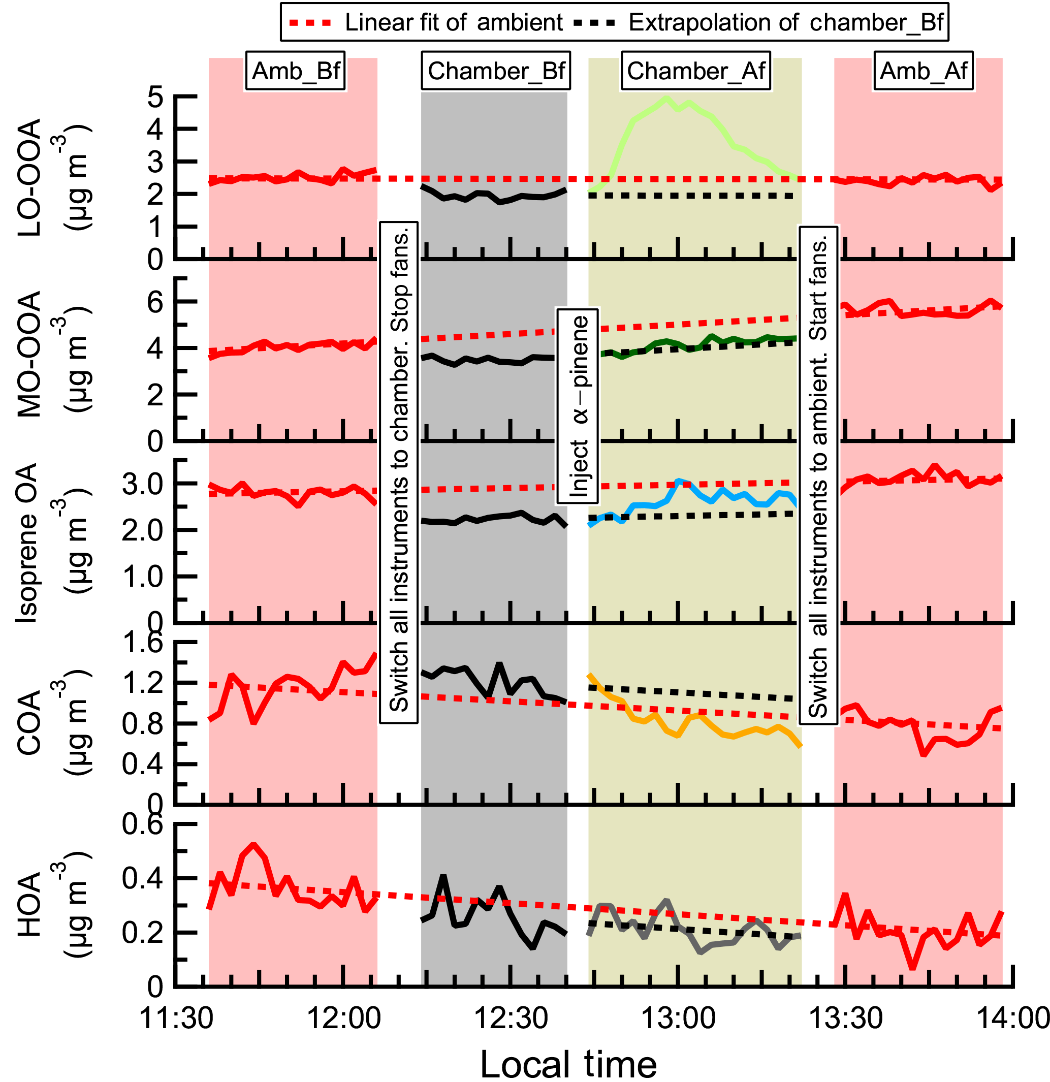
Figure 3The time series of OA factors in an α-pinene perturbation experiment (expt. ID: ap_0801_1). Each perturbation experiment includes four periods: Amb_Bf (∼30 min), Chamber_Bf (∼30 min), Chamber_Af (∼40 min), and Amb_Af (∼40 min). “Amb” and “Chamber” represent the fact that instruments are sampling ambient and chamber, respectively. “Bf” and “Af” stand for before and after perturbation, respectively. The solid lines are measurement data. The dashed red lines are the linear fits of ambient data (i.e., combined Amb_Bf and Amb_Af). The slopes are used to extrapolate Chamber_Bf data to the Chamber_Af period (i.e., dashed black lines). The validity of the linearity assumption is discussed in Appendix A. The difference between measurements (i.e., solid lines) and extrapolated Chamber_Bf (i.e., dashed black lines) represents the change caused by perturbation.
3.1 α-pinene perturbation experiments
A total of 19 α-pinene perturbation experiments were performed at different times of the day (i.e., from 09:00 to 21:00 local time) to probe a wide range of reaction conditions. The injection time and concentrations of O3 and NOx during α-pinene perturbation experiments are summarized in Table S4. Based on the chamber volume and injected liquid α-pinene volume (0.2 µL), initially ∼14 ppb of α-pinene is injected into the chamber. Due to a lack of VOC measurements, we build a box model to simulate the fate of α-pinene in the chamber (Sect. S6 of the Supplement). We estimate that roughly 10 % of α-pinene is reacted in the chamber and most of the α-pinene is carried out of the chamber due to dilution with ambient air.
Figure 3 shows the time series of OA factors in a typical α-pinene perturbation experiment. An evident burst and increase in LO-OOA after α-pinene injection occurs. This provides direct evidence that freshly formed α-pinene SOA contributes to LO-OOA. About 15 min after α-pinene injection, LO-OOA concentration starts to decrease, as ambient air continuously flows into the chamber and dilutes the concentration of LO-OOA (Sect. S6 of the Supplement). As shown in Fig. S3, the major known gas-phase oxidation products of α-pinene measured by HR-ToF-CIMS (Eddingsaas et al., 2012b; Lee et al., 2016; Yu et al., 1999) show an immediate increase after α-pinene injection. This verifies the rapid oxidation of α-pinene in the chamber.
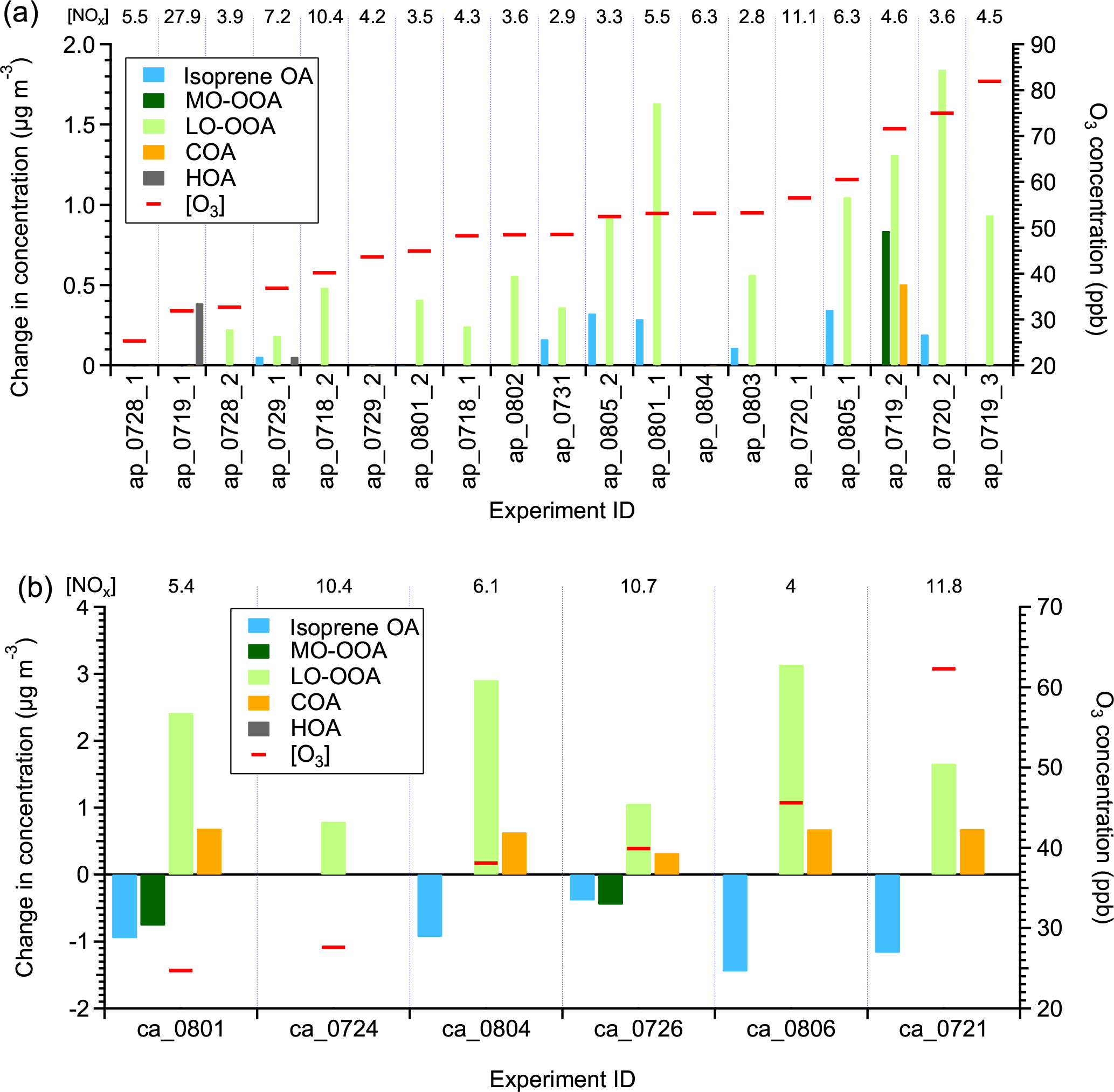
Figure 4The statistically significant changes in the concentrations of OA factors after perturbation by (a) α-pinene and (b) β-caryophyllene. The experiments are sorted by average [O3] during Chamber_Af. The average [NOx] values during Chamber_Af are shown on top of the figure. The changes in concentration are the differences between measurements during Chamber_Af and extrapolated Chamber_Bf (Appendix A). A set of criteria are developed to evaluate if the changes are statistically significant and if the changes are due to ambient variation (Appendix A). Isoprene OA decreases after β-caryophyllene injection. The reason for this decrease is unclear, but likely due to the limitations of PMF analysis, which assumes constant mass spectra of OA factors over time (Sect. S3 of the Supplement).
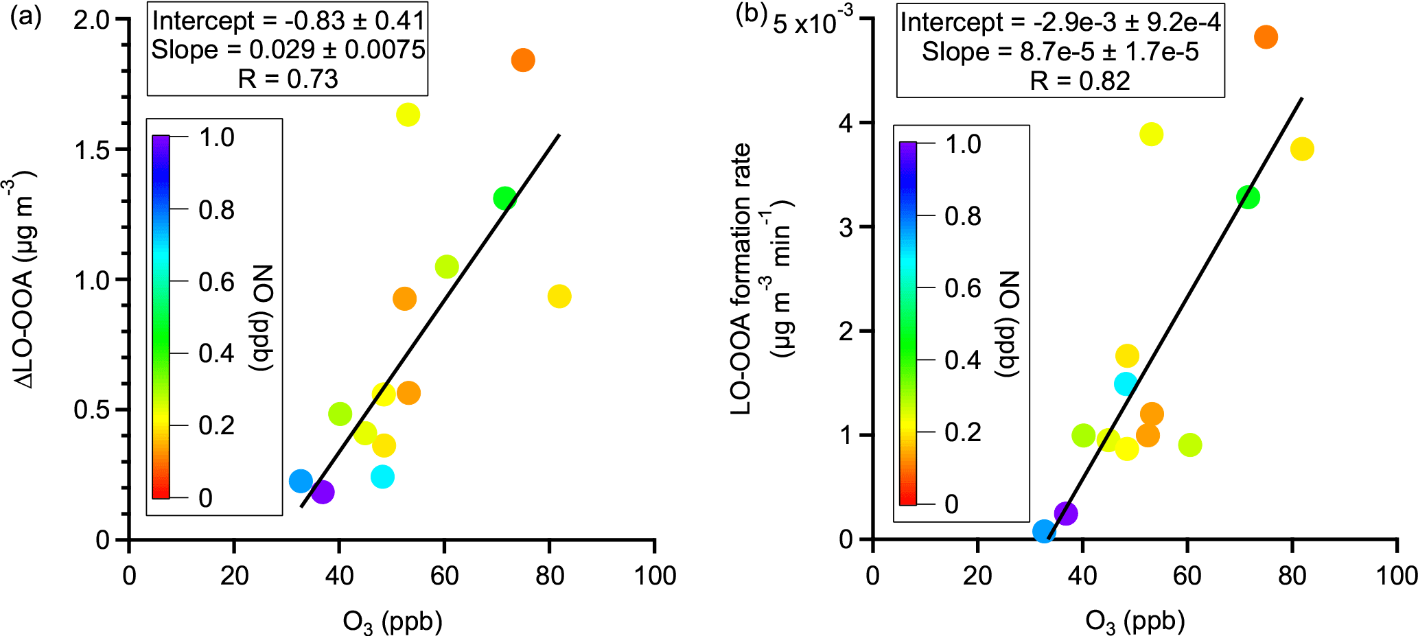
Figure 5Observations of trends in (a) LO-OOA enhancement amount and (b) LO-OOA formation rate with O3 concentration in α-pinene perturbation experiments. The data points are colored by average NO concentration during the Chamber_Af period. The slopes, intercepts, and correlation coefficients (R) are obtained by a least squares fit.
Figure 4a shows the perturbation-induced changes in the concentrations of OA factors for all α-pinene experiments. Out of 19 experiments, the LO-OOA concentration is enhanced in 14 experiments. Also, among all OA factors, LO-OOA shows the largest enhancement. This directly supports the hypothesis that freshly formed α-pinene SOA contributes to LO-OOA. The enhancement in LO-OOA concentration differs between experiments, mainly because the perturbations were performed at different times of day (i.e., from 09:00 to 21:00) and with different reaction variables (i.e., temperature, relative humidity, oxidants concentrations, NOx, etc.). Despite the large difference in reaction conditions, we note that both the LO-OOA enhancement amount and LO-OOA formation rate (i.e., slope of LO-OOA increase) correlate positively with ozone concentration (Fig. 5). This correlation suggests that the concentrations of oxidants, both ozone and the hydroxy radical (OH, which is not measured in this study but is known to positively correlate with ozone in the atmosphere), play a more controlling role in the amount of OA formed in the α-pinene experiment than other reaction variables. This is likely because higher oxidant concentrations lead to more α-pinene consumption and hence more OA production with the same reaction time.
MO-OOA only increases in 1 out of 19 α-pinene experiments. Highly oxygenated molecules (HOMs), which are rapidly produced from the oxidation of α-pinene, are a hypothesized source of MO-OOA because of the high O : C ratio of HOMs (Ehn et al., 2014; Mutzel et al., 2015). However, HOMs are first-generation monoterpene products co-formed with semi-volatile SOA species, and the lack of enhancement in MO-OOA suggests that HOMs are unlikely contributors to MO-OOA. We cannot rule out the possibility that HOMs are not formed under our experimental conditions, and future studies on the simultaneous verification of HOM formation and the apportionment of HOMs by PMF analysis are warranted.
Isoprene-derived OA (isoprene OA) increases in 7 out of 19 α-pinene experiments. This increase is surprising because the isoprene OA factor (also referred to as IEPOX-OA in some studies) is typically interpreted as SOA from the reactive uptake of IEPOX, but our results suggest that the isoprene OA factor could have interferences from α-pinene SOA. The isoprene OA enhancement is due to interference from newly formed α-pinene SOA, rather than the injected α-pinene affecting the oxidation of preexisting isoprene or affecting the gas–particle partitioning of preexisting semi-volatile species in the chamber, for the following reasons. Firstly, based on I− HR-ToF-CIMS measurements, the concentration of isoprene oxidation products, such as IEPOX + ISOPOOH () and isoprene hydroxyl nitrates (), did not change after α-pinene injection (Fig. S3b). In addition, after injecting α-pinene, the increase in SOA concentration is less than 4 µg m−3, which does not substantially perturb the gas–particle partitioning of preexisting semi-volatile species. Finally, the time series of isoprene OA and LO-OOA in the same α-pinene perturbation experiment is strongly correlated (Fig. S4a). It is well studied that isoprene produces SOA at a slower rate than α-pinene, as isoprene SOA involves higher-generation products. If the enhancement in the isoprene OA factor is due to isoprene oxidation, the enhancement of isoprene OA is expected to occur later than the enhancement of LO-OOA, but this is not observed in the experiments. Thus, the strong correlation between isoprene OA and LO-OOA in the same α-pinene perturbation experiment serves as further evidence that the enhancement in the isoprene OA factor is due to interference from newly formed α-pinene SOA rather than the oxidation of isoprene after injecting α-pinene.
The interference of α-pinene SOA on the isoprene OA factor helps to address some uncertainties regarding the isoprene OA factor in the literature. For example, Liu et al. (2015) compared the mass spectrum of laboratory-derived IEPOX SOA with isoprene OA factors at some sites. The authors observed a stronger correlation for isoprene OA factors resolved at Borneo (Robinson et al., 2011a) and the Amazon (Chen et al., 2015) and a weaker correlation at Atlanta, US (Budisulistiorini et al., 2013), and Ontario, Canada (Slowik et al., 2011). As another example, the fraction of measured total IEPOX SOA molecular tracers in the isoprene OA factor highly varies with location, ranging from 26 % at Look Rock, TN (Budisulistiorini et al., 2015) to 78 % at Centreville, AL (Hu et al., 2015). To address the uncertainties in the above two examples, one possible reason is that the isoprene OA factors resolved at different sites are not purely from IEPOX uptake. Isoprene OA factors likely have interference from monoterpene SOA or other sources, but the interference magnitude varies with location.
While the perturbation experiments clearly point out the possibility that the isoprene OA factor could have interference from α-pinene SOA, three caveats should be kept in mind. First, in this study, the enhancement magnitude of isoprene OA is ∼20 % of that of LO-OOA (Fig. S5a), but this interference magnitude would vary with location and season. Second, the perturbation experiments simulate a period with increasing α-pinene SOA concentration. The applicability of the conclusions drawn from this specific scenario to the general atmosphere with more dynamic variations of OA sources warrants further exploration. Third, the perturbation experiments are conducted at ground level, whereas evidence from aircraft studies suggests that the production of isoprene SOA may be stronger at the top of the boundary layer (Allan et al., 2014).
Primary OA factors, i.e., HOA and COA, only show slight increases in one or two α-pinene experiments, indicating a lack of interference from α-pinene SOA in these factors.
3.2 β-caryophyllene perturbation experiments
A total of six β-caryophyllene perturbation experiments were performed; 0.2 µL of β-caryophyllene is injected into the chamber, corresponding to a mixing ratio of 10 ppb. The concentrations of O3 and NOx during β-caryophyllene perturbation experiments are summarized in Table S4. In all β-caryophyllene perturbation experiments, LO-OOA also shows a significant enhancement (Fig. 4b). This clearly shows that freshly formed SOA from β-caryophyllene oxidation can be another source of LO-OOA. In addition to LO-OOA, COA shows an unexpected increase in five out of six β-caryophyllene experiments. We have ample evidence that the COA factor at the measurement site has contributions from cooking activities. Firstly, the diurnal variation of COA peaks during mealtimes (Fig. S6a). Additionally, the COA concentration shows a clear increase on football days, consistent with barbecue activities on campus and close to the measurement site. Finally, the COA concentration is enhanced on the days right before the start of a new semester when there are many fraternity and sorority rush events (i.e., barbecue activities) on campus (Fig. S6b and c). However, the COA enhancement in β-caryophyllene experiments underscores the fact that COA may not be purely from cooking activities in areas with large biogenic emissions.
3.3 Perturbation experiments with other VOCs
In addition to α-pinene and β-caryophyllene, we also performed a few perturbation experiments by injecting isoprene, m-xylene, or naphthalene. However, SOA formation from these VOCs is not detectable. This is mainly due to either lower SOA yields (of isoprene) or slower oxidation rates (of m-xylene and naphthalene) compared to α-pinene and β-caryophyllene, which are discussed in Sect. S6 of the Supplement.
We have also performed four perturbation experiments by injecting acidic sulfate particles to probe the reactive uptake of IEPOX. We observed an enhancement in isoprene OA concentration after the injection of sulfate particles. The detailed results are included in Appendix B.
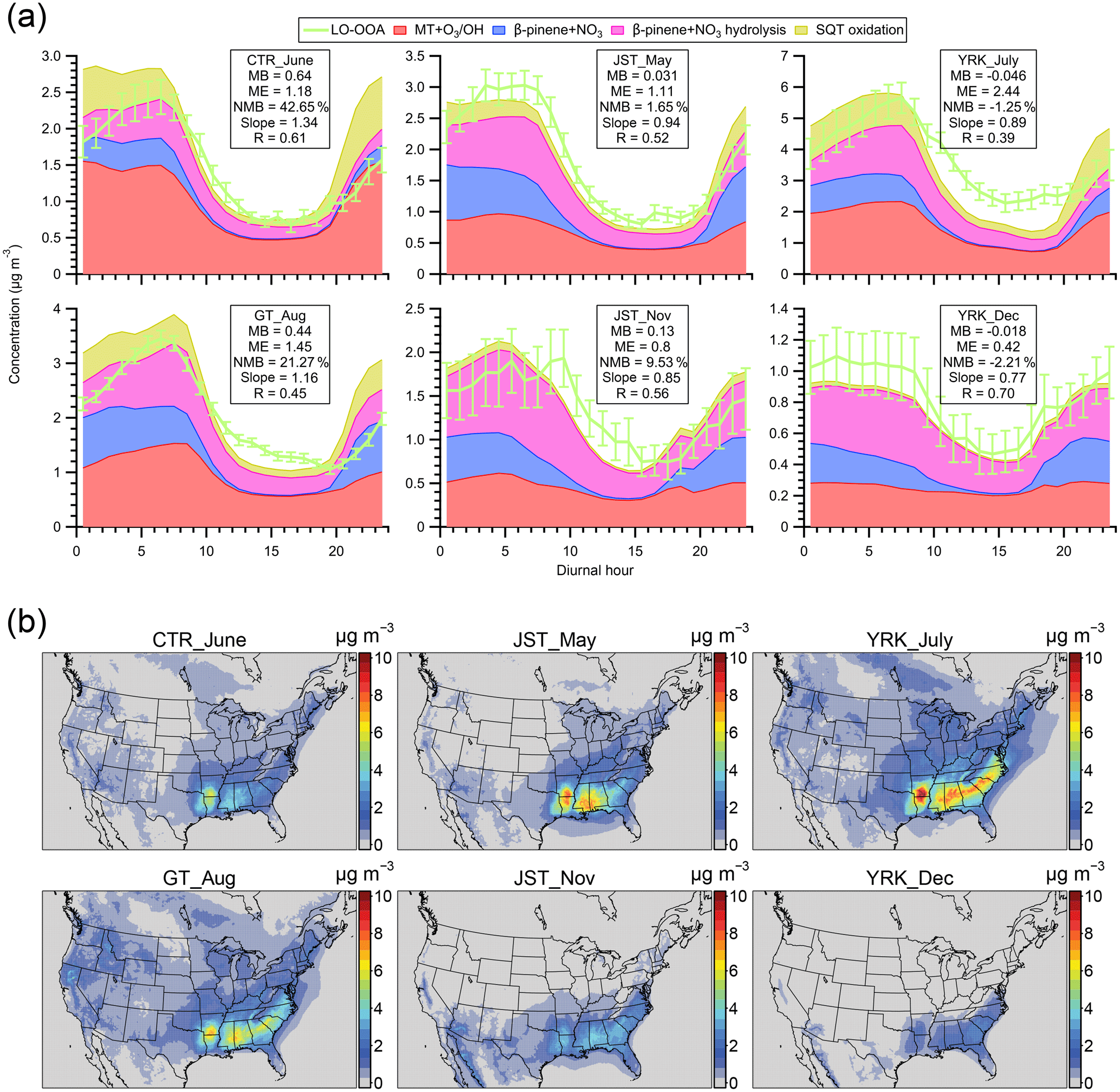
Figure 6(a) The diurnal trends of LO-OOA and modeled SOA from monoterpenes and sesquiterpenes (SOAMT+SQT) at different sampling sites in the southeastern US. (b) Maps of the modeled ground-level SOAMT+SQT concentration coinciding with the time periods of intensive ambient sampling. Model results shown here are from the updated simulation. Abbreviations correspond to Centreville (CTR), Jefferson Street (JST), Yorkville (YRK), and Georgia Institute of Technology (GT). Detailed sampling periods are shown in Table S1. In panel (a), since the perturbation experiments show that 16 % of SOA from α-pinene oxidation is apportioned into isoprene OA (Fig. S5a), we only include 84 % of modeled SOA from MT + O3 ∕ OH when comparing with LO-OOA for the sites with isoprene-OA. The mean bias (MB), mean error (ME), and normalized mean bias (NMB) for each site are shown in each panel. The slopes and correlation coefficients (R) are obtained by a least squares fit. The error bars indicate the standard error. In panel (b), the average SOAMT+SQT concentration in PM2.5 during each sampling period is reported.
3.4 LO-OOA as a surrogate of SOAMT+SQT in the southeastern US
We propose that the major source of LO-OOA in the southeastern US is fresh SOA from the oxidation of MT and SQT by various oxidants (O3, OH, and NO3) based on multiple lines of evidence. First, the southeastern US is characterized by large biogenic emissions, including monoterpenes and sesquiterpenes (Guenther et al., 2012). Second, the majority of carbon in SOA is modern in the southeastern US. Weber et al. (2007) measured the biogenic fraction of SOA to be roughly 70 %–80 % at two urban sites in Georgia that were also used in our study. We note that the measurements in Weber et al. (2007) were performed in 2004 and the biogenic fraction of SOA is expected to be higher in 2016 than 2004 as a result of reductions in anthropogenic emissions (Blanchard et al., 2010). Third, previous studies suggest that the oxidation of β-pinene (another important monoterpene) by nitrate radicals (NO3) contributes to LO-OOA in the southeastern US (Boyd et al., 2015; Xu et al., 2015a), though this reaction alone cannot replicate the magnitude of LO-OOA (Pye et al., 2015). Fourth, the mass spectra of LO-OOA are almost identical (i.e., R ranges from 0.95 to 0.99 in Fig. S7) across all the seven datasets in our study. In addition, LO-OOA across all datasets also shares the same diurnal trends (Xu et al., 2015a). The similarity in LO-OOA features suggests that LO-OOA generally shares similar sources across multiple sites and in different seasons in the southeastern US. Fifth, the lab-in-the-field perturbation experiments provide objective evidence that the majority of freshly formed SOA from the oxidation of MT and SQT contributes to LO-OOA. Sixth, using the updated CMAQ model (i.e., explicit organic nitrates and Saha and Grieshop, 2016, VBS for MT + O3 ∕ OH SOA), we found that the simulated SOAMT+SQT reasonably reproduces both the magnitude and diurnal variability of LO-OOA for all sites (Fig. 6a). The model bias is within ∼20 % for most sites, except for Centreville, Alabama (i.e., 43 % for CTR_June dataset). Figure 6b presents maps of ground-level SOAMT+SQT concentration corresponding to the time periods of observational data, and the SOAMT+SQT concentration is substantially higher in the southeast than other US regions. While SOAMT+SQT is present throughout the year, it reaches the largest concentration in summer. The spatial and seasonal variation of the SOAMT+SQT concentration is consistent with MT and SQT emissions (Guenther et al., 2012). The consistency between modeled SOAMT+SQT and measured LO-OOA at multiple sites and in different seasons builds confidence in our hypothesis that LO-OOA largely arises from the oxidation of MT and SQT in the southeastern US.
We note that we do not conclude that LO-OOA arises exclusively from MT and SQT. SOA from other precursors or other pathways may contribute to LO-OOA, but the related contributions are expected to be much smaller than MT and SQT in the southeastern US. Firstly, the contributions of anthropogenic SOA to LO-OOA are likely small. The emissions of anthropogenic VOCs are much weaker than those of biogenic VOCs in the southeastern US (Goldstein et al., 2009). We modeled the concentration of anthropogenic SOA to be on the order of 0.1 µg m−3 for our datasets (Fig. S8). Even if we double the SOA yields of anthropogenic VOCs to account for the potential vapor wall loss in laboratory studies (Zhang et al., 2014), the concentration of SOA from anthropogenic VOC oxidation is still negligible compared to SOAMT+SQT. The low modeled concentration of anthropogenic SOA is consistent with Zhang et al. (2018), who showed that the measured tracers of anthropogenic SOA only account for 2 % of total OA in Centreville, AL. Secondly, other reaction pathways, like aqueous-phase chemistry or some unexplored reaction, may contribute to LO-OOA. However, the consistency between modeled SOAMT+SQT and LO-OOA suggests that LO-OOA can be reasonably represented by a model based on current knowledge. In addition, SOA produced from aqueous-phase chemistry is generally highly oxidized (Lee et al., 2011) and may be apportioned into MO-OOA instead of LO-OOA. A recent study by W. Xu et al. (2017) suggests that aqueous-phase SOA is a major source of MO-OOA in China.
We limit our hypothesis that the major source of LO-OOA is the oxidation of MT and SQT to the southeastern US. The southeastern US is a unique location in that there have been a large number of field studies in recent years at multiple locations and seasons throughout the region. Results from these studies provided additional constraints for OA sources in this region (Carlton et al., 2018; Zhang et al., 2018; Xu et al., 2015a; Warneke et al., 2016). At other locations, there is evidence that the LO-OOA factor represents different sources. For example, radiocarbon analysis shows that 68 %–75 % of carbon in LO-OOA in California stems from fossil sources (Hayes et al., 2013; Zotter et al., 2014), suggesting a contribution from anthropogenic SOA to LO-OOA. Also, in the wintertime of many locations, LO-OOA and MO-OOA are not separated and a single OOA factor is resolved (Xu et al., 2016b; Lanz et al., 2008). Further developments are needed if one were to use the perturbation experimental approach for source apportionments of OA at other sites if auxiliary constraints from field measurements, laboratory studies, and/or modeling are not readily available for those sites.
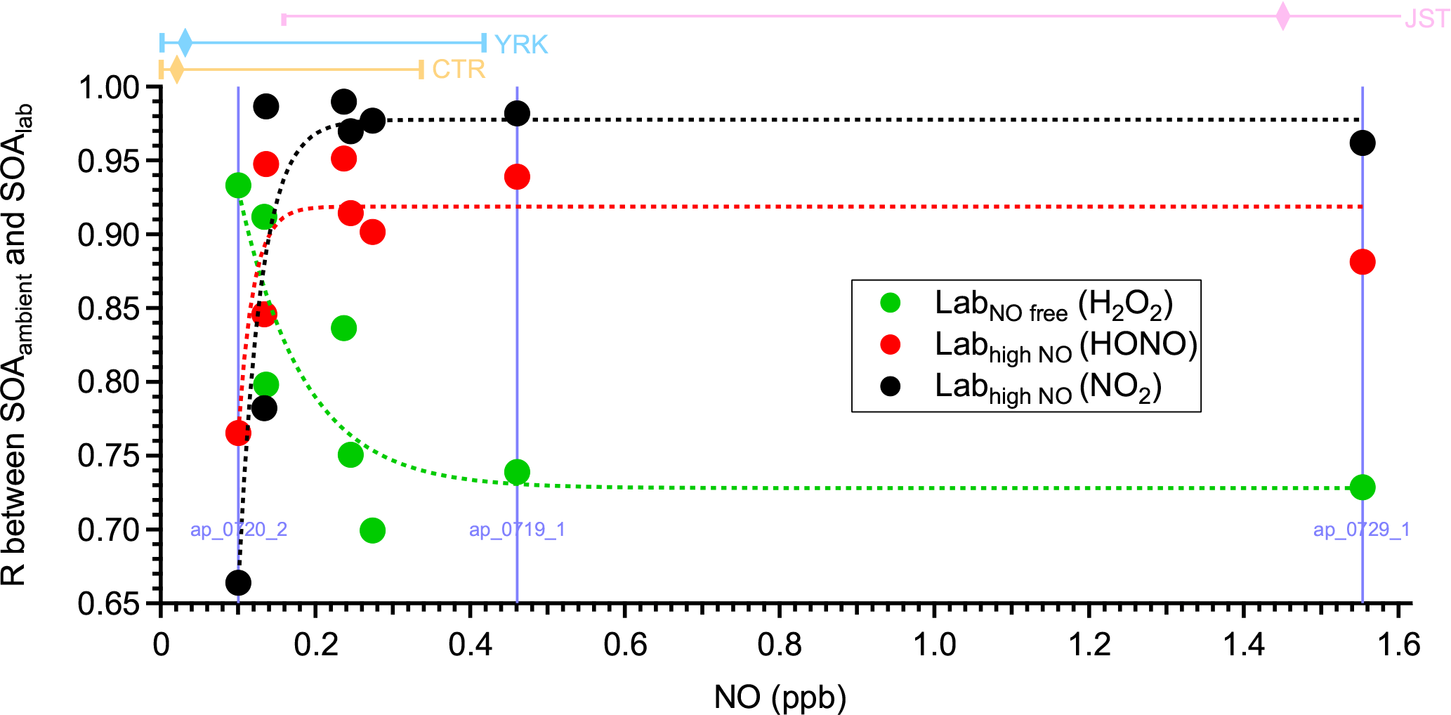
Figure 7The correlation coefficients between the mass spectra of OA formed in the laboratory under different NO conditions (SOAlab) and those of OA formed in ambient α-pinene perturbation experiments (SOAambient). The subscripts lab and ambient indicate the SOA formed under laboratory conditions and ambient conditions, respectively. Three different oxidant sources (i.e., H2O2, HONO, and NO2) are used to create different NO concentrations in laboratory studies. The mass spectra of SOAambient are calculated by comparing the mass spectra of OA during Chamber_Af and those of extrapolated Chamber_Bf (Sect. S7 of the Supplement). To calculate reliable mass spectra of SOAambient, only the experiments with significant OA enhancement are analyzed and shown here (Appendix A). The x axis is the average NO concentration during each perturbation experiment. The data points on the same vertical line (i.e., the same NO concentration) are from the same perturbation experiment, but compared to three different laboratory experiments. The dashed lines are used to guide the eyes. The bars on top of the figure represent the 10th, 50th, and 90th percentiles of NO concentration for CTR (Centreville, AL), YRK (Yorkville, GA), and JST (Jefferson Street, GA) in 2013. The NO concentration is measured by the Southeastern Aerosol Research and Characterization (SEARCH) network. The 90th percentile of NO concentration in JST is 14.8 ppb, which is not shown in the figure.
3.5 Connection between laboratory and field studies
Due to the difficulties associated with accurately measuring complex chemical processes in the atmosphere, laboratory studies have been an integral part in our understanding of atmospheric chemistry (Burkholder et al., 2017). However, the representativeness of laboratory studies under simplified conditions with respect to the complex atmosphere is difficult to evaluate. One unique feature of our lab-in-the-field approach is that VOC oxidation and SOA formation proceed under realistic atmospheric conditions. Taking advantage of this, we provide a direct link between laboratory studies and ambient observations. Previous laboratory studies have shown that NO can affect SOA composition by influencing the fate of the organic peroxy radical (RO2, a critical radical intermediate formed from VOC oxidation) (Kroll and Seinfeld, 2008; Sarrafzadeh et al., 2016; Presto et al., 2005). To evaluate the representativeness of laboratory studies and investigate the effects of NO on SOA composition, in Fig. 7 we compare the chemical composition of α-pinene SOA formed in laboratory studies under different NO conditions (denoted as SOAlab) with those in α-pinene ambient perturbation experiments (denoted as SOAambient). The degree of similarity in OA mass spectra (i.e., evaluated by the correlation coefficient) between laboratory α-pinene SOA generated under NO-free conditions (i.e., denoted as SOAlab,NO-free, using H2O2 photolysis as oxidant source) and SOAambient shows a strong dependence on the ambient NO concentration under which SOAambient is formed. The degree of similarity in mass spectra decreases rapidly when ambient NO increases from 0.1 to 0.2 ppb, and then reaches a plateau at ∼0.3 ppb NO. The opposite trend is observed when laboratory α-pinene SOA generated in the presence of high NO concentrations (i.e., denoted as SOAlab,high-NO, using the photolysis of NO2 or nitrous acid as an oxidant source) is compared with SOAambient. These observations show the transition of RO2 fate as a function of NO under ambient conditions. For the perturbation experiments performed when ambient NO is below ∼0.1 ppb, the mass spectra of SOAambient are similar to SOAlab,NO-free, consistent with the fact that RO2 mainly reacts with hydroperoxyl (HO2) or isomerizes. In contrast, for the perturbation experiments performed when ambient NO is above ∼0.3 ppb, the mass spectra of SOAambient are similar to SOAlab,high-NO. This NO level (∼0.3 ppb) is consistent with the NO level required to dominate the fate of RO2 in the atmosphere, as calculated by using previously measured HO2 and kinetic rate constants (Sect. S8 of the Supplement). The unimolecular reactions of RO2 are not considered. These observations also illustrate that the SOA composition from laboratory studies can be representative of the atmosphere. We note that the mass spectra of SOAambient are generally more similar with those of laboratory SOA generated using NO2 photolysis as an oxidant source than using nitrous acid photolysis. This suggests that laboratory experiments using NO2 photolysis as an oxidant source better represent ambient high NO oxidation conditions in the southeastern US than experiments using nitrous acid. Possible explanations are discussed in Sect. S7 of the Supplement. This finding provides new insights into designing future laboratory experiments to better mimic the oxidations in ambient environments.
In this study, we performed lab-in-the-field perturbation experiments and provided objective evidence that the majority of fresh SOA from the oxidation of MT and SQT contributes to LO-OOA. Based on multiple lines of evidence, we propose that LO-OOA can be used as a surrogate for fresh SOA from MT and SQT in the southeastern US. We showed that modeled SOAMT+SQT could reasonably reproduce both the magnitude and diurnal variability of LO-OOA at different sites and in different seasons. Based on the model simulation, we estimate that the annual concentration of SOAMT+SQT to PM2.5 in the southeastern US is ∼2 µg m−3 (i.e., average concentration over the six sampling periods and over the southeastern US in the updated simulation). This accounts for 20 % of the World Health Organization PM2.5 guideline (i.e., 10 µg m−3 annual mean) and indicates a significant contributor of environmental risk to the 77 million habitants in the southeastern US. Also, the estimated abundance of SOAMT+SQT is substantially larger than represented in current models (Lane et al., 2008; Zheng et al., 2015), but in line with the conclusion from Zhang et al. (2018). Zhang et al. (2018) used a different methodology, characterization of molecular tracers of MT SOA at Centreville, AL (a site included in our study as well), to conclude that monoterpenes are the largest source of summertime organic aerosol in the southeastern US. The oxidation of MT and SQT is likely an underestimated contributor to PM in the present day and perhaps during the preindustrial period, which determines the baseline state of the atmosphere and the estimate of climate forcing by anthropogenic emissions (Carslaw et al., 2013). Models need to improve the description of MT and SQT oxidation to reduce the uncertainties in the estimated OA budget and subsequent climate forcing.
Using LO-OOA as a surrogate for SOAMT+SQT in the southeastern US, our ambient ground measurements suggest that at least 19 %–34 % of OA in the southeastern US is from the oxidation of biogenic monoterpenes and sesquiterpenes (Xu et al., 2015a). The fraction of biogenic OA in the southeastern US is even larger if we consider the fact that isoprene OA could account for 21 %–36 % of OA in summer (despite potential interferences of SOA from monoterpene oxidation) and that MO-OOA (24 %–49 % of OA) likely contains SOA from the long-term photochemical oxidation of biogenic VOCs. The dominant biogenic origin of SOA poses a challenge to control its burden in the southeastern US if the roles of anthropogenic oxidants and other controlling factors are not recognized. Previous studies have shown that SOA formation from biogenic VOCs can be mediated by anthropogenic emissions, such as nitrogen oxides and sulfur dioxide (Hoyle et al., 2011; Goldstein et al., 2009; Surratt et al., 2010; Rollins et al., 2012; Xu et al., 2015a). Thus, regulating anthropogenic emissions could help reduce the SOA concentration (Lane et al., 2008; Pye et al., 2015; Zheng et al., 2015). For example, as observed in our ambient perturbation experiments, one controlling parameter of α-pinene SOA formation is the concentration of atmospheric oxidants (O3, OH, and NO3), which are known to strongly depend on NOx concentration. As it has been shown that anthropogenic emissions exert complex and nonlinear influences on biogenic SOA formation (Zheng et al., 2015), the effectiveness of regulating anthropogenic emissions on the biogenic SOA burden requires careful investigations.
Data can be obtained by request (ng@chbe.gatech.edu).
The most challenging and important analysis is to determine if the perturbation causes a statistically significant change in the mass concentration of OA factors. We perform the following analysis to calculate the changes in the mass concentration of OA factors after perturbation to determine if the change is significant and to evaluate if the change is simply due to ambient variation.
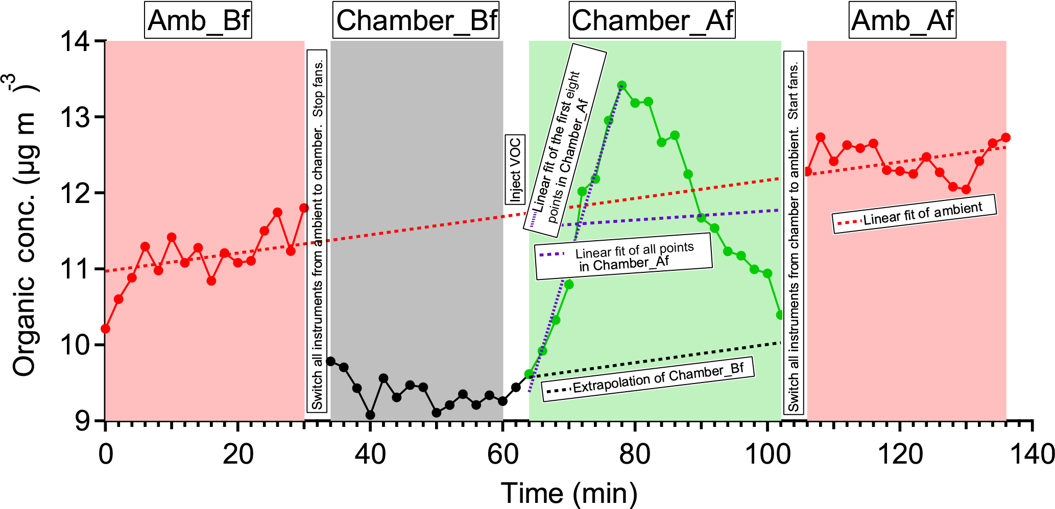
Figure A1Time series of OA in experiment ap_0801_1 to illustrate the analysis method. Each perturbation experiment includes four periods: Amb_Bf (∼30 min), Chamber_Bf (∼30 min), Chamber_Af (∼40 min), and Amb_Af (∼40 min). “Amb” and “Chamber” correspond to the periods when the instruments are sampling ambient and chamber, respectively. “Bf” and “Af” stand for before and after perturbation, respectively. The solid lines are measurement data. The dashed red lines are the linear fit of ambient data (i.e., combined Amb_Bf and Amb_Af). The slope is used to extrapolate Chamber_Bf data to the Chamber_Af period (i.e., black dashed line). The dense dashed purple line is the linear fit of the first eight points during the Chamber_Af period. The sparse dashed purple line is the linear fit of all data points during the Chamber_Af period. During this period, the difference between measurements (i.e., solid green data points) and extrapolated Chamber_Bf (i.e., dashed black line) represents the change in organic concentration caused by perturbation.
The duration of one perturbation experiment is about 130 min, including four periods: Amb_Bf (∼30 min), Chamber_Bf (∼30 min), Chamber_Af (∼40 min), and Amb_Af (∼30 min), as illustrated in Fig. A1. Firstly, we assume that the ambient variation is linear during both the Chamber_Bf and Chamber_Af periods (i.e., when instruments are connected to the chamber and not sampling the ambient aerosol) and that the ambient variation can be represented by interpolating Amb_Bf and Amb_Af. The validity of this assumption will be discussed shortly. To obtain the slope of ambient variation, we analyze the combined Amb_Bf and Amb_Af data and use a Theil–Sen estimator (Sen, 1968). The Theil–Sen estimator is a method to robustly fit a line to a set of two-dimensional points (i.e., concentration C and time t in this study). This method chooses the median of the slopes determined by all pairs of sample points. Compared to simple linear regression using ordinary least squares, the Theil–Sen estimator is robust and insensitive to outliers. Unless specifically noted, the slope in Appendix A is calculated from the Theil–Sen estimator. Secondly, we use the slope to extrapolate the Chamber_Bf data to estimate aerosol concentration inside the chamber during the Chamber_Af period if there were no VOC injection. We refer to this estimated aerosol concentration as “extrapolated Chamber_Bf” and use it as the reference to calculate the change in aerosol mass concentration after perturbation. We extrapolate the Chamber_Bf data, instead of ambient data, because the OA concentration in the chamber is lower than that in the atmosphere due to wall loss. Thirdly, we calculate the changes in the concentration of OA factors based on the difference between measured Chamber_Af data and extrapolated Chamber_Bf.
For each perturbation experiment, after calculating the changes in the concentration of OA factors, we develop a set of criteria to determine if the changes are statistically significant and if the changes are simply due to ambient variation. The increase in the concentration of an OA factor needs to satisfy all criteria to be considered as statistically significant and not due to ambient variation.
Criterion 1: the difference in concentration between Chamber_Af and extrapolated Chamber_Bf must be significant. We use a T test and the 95 % confidence interval.
Criterion 2: the slope of all data points or the first eight data points during the Chamber_Af period is significantly different from the slope of the aerosol concentration during the Chamber_Bf period. The rationale behind this criterion is that if the perturbation causes a substantial change in the concentration of an OA factor, its slope during the Chamber_Af period should be different from that during the Chamber_Bf period.
The slope of the aerosol concentration during the Chamber_Af period is obtained in the following way. We calculate the slope by using (1) all data points and (2) only first eight data points during the Chamber_Af period. This is because the concentration of factors firstly increases after perturbation and then decreases due to dilution (Fig. A1). In this case, the slope obtained by fitting all data points might be negative and will not reflect the initial increase in concentration (e.g., LO-OOA of ap_0805_1 in Fig. S9a). Using only the first few data points during the Chamber_Af period can avoid this issue. We select the first eight data points in this period because the concentrations of total OA and OA factors typically reach the highest at the eighth point (i.e., ∼16 min after injection). The slope is calculated by the Theil–Sen estimator.
The slope of aerosol concentration during the Chamber_Bf period is analyzed in the following way. In order to determine if the slope in Chamber_Af is significantly different from that in Chamber_Bf, we use bootstrap analysis (1000 times) to obtain a distribution of the slope of Chamber_Bf. In brief, in each random resampling of Chamber_Bf with replacement, a slope is calculated by the Theil–Sen estimator. Then, 1000 resamplings provide a distribution of the slope in Chamber_Bf. The 5th and 95th percentiles of the slope distribution are compared to the slope of Chamber_Af to determine if the slopes are significantly different. If the slope of Chamber_Af (from either all data points or the first eight data points) is smaller (or larger) than the 5th (or 95th) percentile, the slopes in Chamber_Bf and Chamber_Af are significantly different.
Criterion 3: the slope of all data points or the first eight data points during the Chamber_Af period is significantly different from the slope of ambient data (i.e., combined Amb_Bf and Amb_Af). The rationale behind this criterion is the same as the second criterion. That is, if the perturbation causes a substantial change in the concentration of an OA factor, its slope during the Chamber_Af period should be different from that in ambient data. The procedure to obtain a distribution of slopes in the ambient data (combined Amb_Bf and Amb_Af) is the same as criterion 2.
As mentioned above, one critical assumption is that the ambient variation is linear during both the Chamber_Bf and Chamber_Af periods (i.e., when instruments are connected to the chamber and not sampling the ambient aerosol) and that the ambient variation can be represented by interpolating Amb_Bf and Amb_Af. We design the following pseudo-experiment to test the validity of this assumption. In brief, we perform the same analysis as we did for the perturbation experiments, but using ambient data only (i.e., no perturbation data). We first randomly select a data point, which defines the start point of one pseudo-test. Secondly, based on the start point, we obtain the concentration of OA factors during the Amb_Bf period (i.e., from start point to start point + 30 min), the Chamber_Bf period (i.e., from start point + 30 min to start point + 60 min), the Chamber_Af period (i.e., from start point + 60 min to start point + 100 min), and the Amb_Af period (from start point + 100 min to start point + 130 min). This mimics the sampling periods in a real perturbation experiment. Thirdly, we calculate the slope of the ambient period (i.e., combined Amb_Bf and Amb_Af periods) and the slope of the chamber period (i.e., combined Chamber_Bf and Chamber_Af periods) in the pseudo-test. Fourthly, we calculate if the slope of the chamber period is significantly different from the slope of the ambient period. We repeat this pseudo-test 1000 times and then obtain the probability of whether the slopes of the chamber period and ambient period are significantly different.
Figure A2a shows the probability that the slopes of the chamber period and ambient period are not significantly different for five factors. The larger this probability is, the more reliable the linearity assumption is. The average probability is ∼50 % for all factors, without discernible diurnal trends. This suggests that there is a ∼50 % chance that the linear variation assumption is valid. Since the linearity assumption is not perfect, we develop another criterion to constrain the potential influence of ambient variation on the interpretation of perturbation results.
Criterion 4: from the above pseudo-experiment on ambient data only, we can calculate the relative change in slope between the “chamber period” and “ambient period” by
In each pseudo-experiment test, we calculate a relative change in slope between the chamber period and ambient period. By repeating the pseudo-experiment test 1000 times, we obtain a frequency distribution of the relative change in slope for each OA factor (Fig. A2b). This frequency distribution indicates the probability that a certain relative change in slope occurs due to ambient variation. Take LO-OOA as an example: the probability that the relative change in slope varies by a factor of 8 due to ambient variation is ∼1 %. Thus, if the relative change in the slope of LO-OOA in an α-pinene experiment is 8, the change is unlikely due to ambient variation. We use the 5th and 95th percentiles from the frequency distribution as the fourth criterion to determine if the changes in the concentrations of OA factors in each perturbation experiment are due to ambient variation. In other words, if the relative change in slope between Chamber_Af and ambient data in a real perturbation experiment falls outside of the 5th or 95th percentiles, the changes in the concentrations of OA factors are likely due to perturbing the chamber with VOC instead of ambient variation. This criterion strictly considers the influence of ambient variation. In general, the comparison in slope is an optimal option to account for ambient variation because the influence of ambient variation is unlikely to coincide with the perturbation.
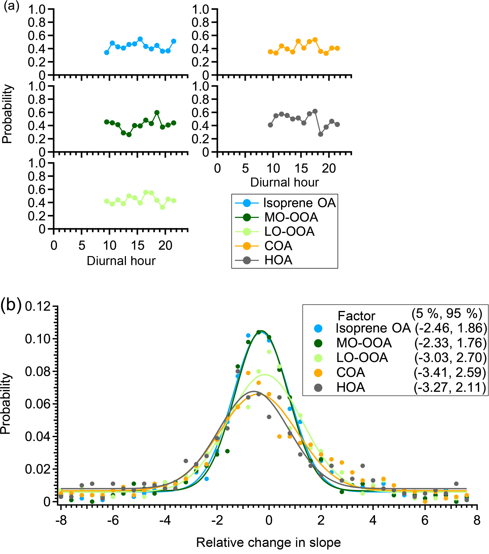
Figure A2(a) The diurnal trends of the probability that the slopes between ambient periods (i.e., Amb_Bf and Amb_Af periods) and chamber periods (i.e., Chamber_Bf and Chamber_Af periods) are not significantly different in the pseudo-experiment. (b) The frequency distribution of the relative change in slope. The data points are fitted using a Gaussian function. The numbers in the box represent the 5th and 95th percentile of the Gaussian fit.
Based on these four criteria, the OA factors with significant changes in their mass concentrations as a result of perturbation are shown in Fig. 4. LO-OOA is enhanced in 14 out of 19 α-pinene experiments. However, total OA is only enhanced in 8 out of 19 α-pinene experiments. Several reasons can contribute to the different behaviors of LO-OOA and OA. Firstly, as total OA has multiple sources, the enhancement in one factor does not guarantee an enhancement of total OA. For instance, in some perturbation experiments, while LO-OOA is enhanced, the concentration of other factors steadily decreases due to ambient variation. The increase in LO-OOA and decrease in other factors compensate for each other and result in a lack of enhancement in total OA. Secondly, based on the pseudo-experiment, we note that total OA is more easily affected by ambient variation than a single OA factor. For example, 95 % of the relative change in the slope of total OA is 3.59, which is larger than any OA factors (Fig. A2b). Thus, the criteria for the change in total OA concentration to be considered as significant are stricter than those for a single OA factor. Thus, some experiments with significant changes in LO-OOA do not have significant changes in total OA.
Previous field observations showed strong correlation between isoprene OA and sulfate (Xu et al., 2015a, 2016a; Budisulistiorini et al., 2015). Moreover, airborne measurements over power plant plumes in Georgia, US, observed enhanced isoprene OA formation in the sulfate-rich power plant plume (Xu et al., 2016a). To probe the relationship between isoprene OA and sulfate, we conducted perturbation experiments in August 2015 by injecting acidic sulfate particles (i.e., a mixture of H2SO4 and MgSO4) into the 2 m3 Teflon chamber. This mimics the airborne measurements over power plants, which introduce sulfate into the atmosphere (Xu et al., 2016a).
The experimental procedure in the 2015 experiments is generally similar to those in the 2016 experiments, but has the following modifications. Firstly, in order to avoid the depletion of species that can uptake to sulfate particles, we kept one fan on during the Chamber_Bf and Chamber_Af periods to enhance the air exchange between the chamber and atmosphere. Secondly, considering that the fan is on during sulfate injection to enhance mixing of the chamber air with ambient air, we only use the Chamber_Bf and Chamber_Af periods to calculate the changes in OA factors. Criteria 1, 2, and 4 are applied in the 2015 experiments. Thirdly, the Chamber_Bf period is ∼40 min in the 2015 experiments, which is slightly longer than the 30 min in the 2016 experiments. Fourthly, the HR-ToF-CIMS was not deployed in the 2015 experiments.
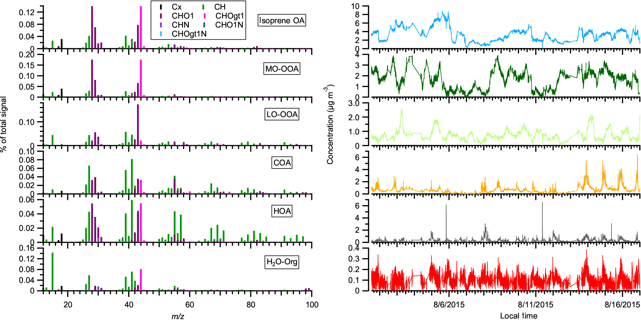
Figure B1The mass spectra and time series of OA factors in the 2015 acidic sulfate particle perturbation measurements. Note that the perturbation periods are included in the time series.
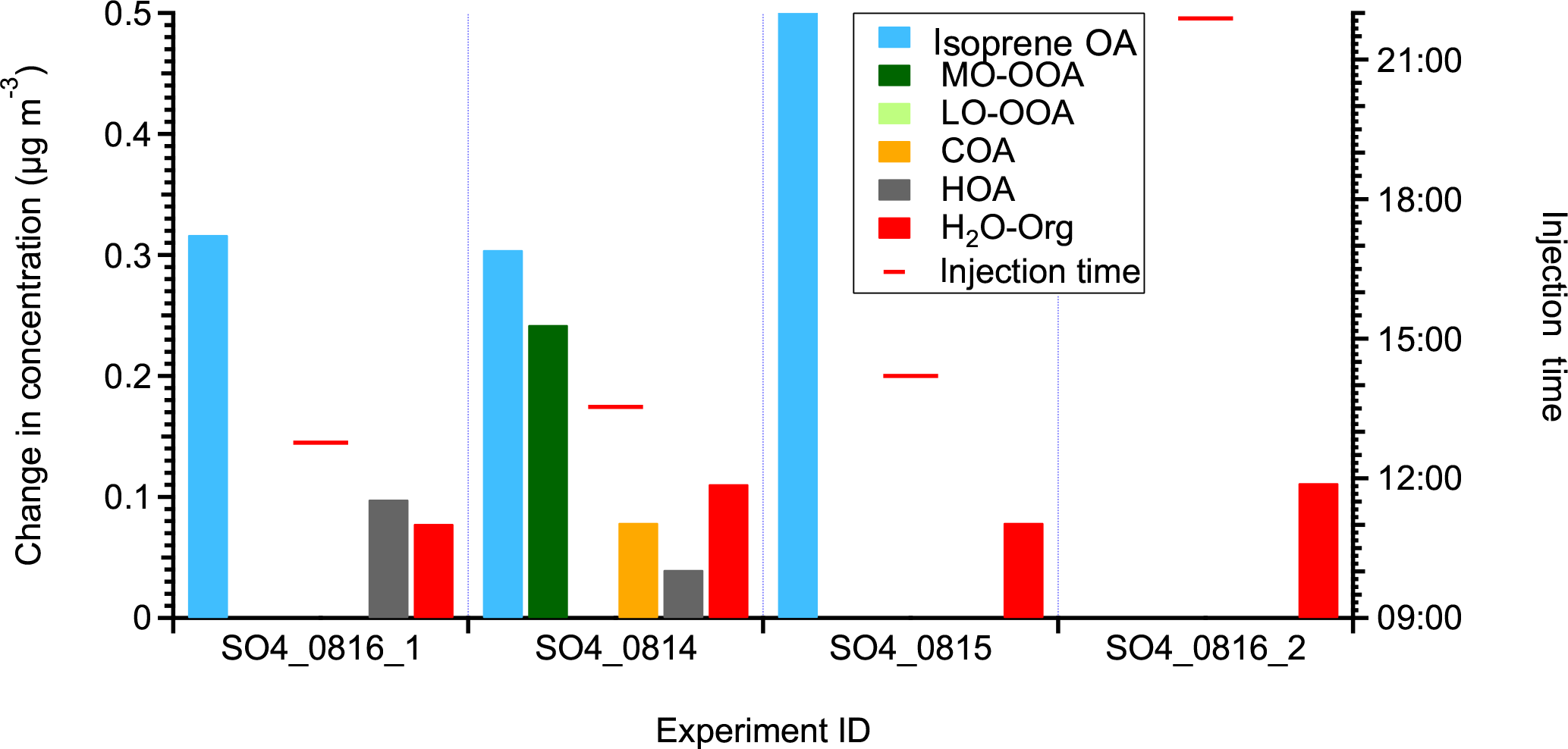
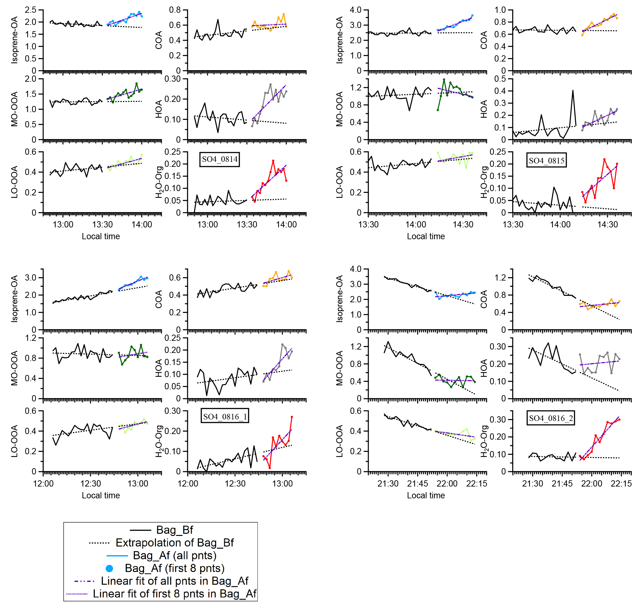
Figure B2The statistically significant changes in the concentrations of OA factors after perturbation by acidic sulfate particles. The experiments are sorted by perturbation time. The changes in concentration are the difference between measurements during the Chamber_Af period and mass concentration extrapolated from the Chamber_Bf period. A set of criteria are developed to evaluate if the changes are significant and if the changes are due to ambient variation (Appendix A). The H2O-Org factor in these sulfate perturbation experiments represents organic contaminations in atomizing water.
Table B1Experimental conditions for sulfate perturbation experiments.
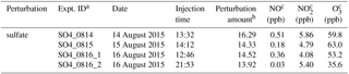
a Expt. ID is “perturbation species + date + experiment number”. For example, SO4_0816_1 represents the first sulfate perturbation experiment on 16 August. b The unit for the perturbation in sulfate experiments is µg m−3. The perturbation amounts of sulfate are calculated from Chamber_Af – extrapolated Chamber_bf. c Average concentration during the Chamber_Af period.
The acidic sulfate seed particles were introduced into the chamber by atomizing 0.88 mM H2SO4 + 0.48 mM MgSO4 mixture solution from a nebulizer (U-5000AT; Cetac Technologies Inc., Omaha, Nebraska, USA). One important interference in these sulfate perturbation experiments is the trace amount of organics in solvent water (i.e., HPLC-grade ultrapure water; Baker Inc.), which is used to prepare the H2SO4 + MgSO4 solution. These organics were injected into the chamber together with sulfate. We utilize the multilinear engine solver (ME-2) to constrain the organics from solvent water (i.e., H2O-Org). Unlike the PMF2 solver, which does not require any a priori information of mass spectrum or time series, the ME-2 solver uses a priori information to reduce rotational ambiguity among possible solutions (Canonaco et al., 2013; Paatero, 1999). We obtained the reference spectrum of organic contamination (i.e., the a priori information for ME-2 solver) by atomizing the H2SO4 + MgSO4 solution directly into AMS. The ME-2 solver successfully extracted a factor (i.e., denoted as the H2O-Org factor, Fig. B1) that showed a clear enhanced concentration during atomization (Fig. B2 and B3).
A total of four experiments were performed and the details are summarized in Table B1. As shown in Fig. B2, the isoprene OA factor increases in all three daytime experiments, but not the nighttime experiment. Based on the current understanding of the isoprene OA factor, this enhancement is likely due to the reactive uptake of IEPOX. The lack of enhancement in the nighttime experiment is consistent with a low IEPOX concentration at night (Hu et al., 2015). Our results provide direct observational evidence that acidic sulfate particles lead to an increase in isoprene OA, which supports results from previous studies (Xu et al., 2015a, 2016a; Budisulistiorini et al., 2015). Due to a lack of measurements of gas-phase organic compounds, we are unable to identify the reactive species. Other species, such as glyoxal (Kroll et al., 2005), isoprene hydroperoxides (Liu et al., 2016), and HOMs (Ehn et al., 2014), also have the potential to uptake to acidic sulfate particles and form SOA. Future experiments with comprehensive measurements of gas-phase organic compounds can provide more insights into the identities of reactive uptake species.
We note that in the non-atomizing period, the concentration of the H2O-Org factor is close to zero, but not zero. Since H2O-Org arises from the atomizing solution, it should only exist during atomizing periods. Thus, the nonzero concentration suggests the limitation of the ME-2 solver and caution is required when using the ME-2 solver to resolve one factor based on a specific mass spectrum. This limitation does not affect the conclusion that the enhancement in isoprene OA is likely due to the reactive uptake of organic species, as we further verify that the organic increase in three daytime perturbation experiments with sulfate particles cannot be solely explained by the organic contamination in atomizing water based on the following two aspects. For example, we atomize the solution directly into AMS and find that the Org∕SO4 ratio is 0.025. This value is significantly lower than the Org∕SO4 ratio in the three daytime sulfate perturbation experiments (i.e., 0.048–0.059), but close to the nighttime sulfate perturbation experiment (i.e., 0.022) (Fig. B4).

Figure B4The Org∕SO4 ratio in sulfate perturbation experiments and laboratory tests by directly atomizing H2SO4 + MgSO4 mixture solution into AMS (i.e., SO4_direct).
The supplement related to this article is available online at: https://doi.org/10.5194/acp-18-12613-2018-supplement.
LX and NLN designed the research. LX and YC performed the research. HOTP and BNM developed and performed the CMAQ simulation. LX, JH, HOTP, BNM, and NLN analyzed the data. LX and NLN wrote the paper. All authors commented on the manuscript.
The authors declare that they have no conflict of interest.
The research has been subjected to EPA review and approved for publication but may not necessarily reflect official EPA policy.
Lu Xu and Nga Lee Ng acknowledge support from the US Environmental Protection Agency
(EPA) STAR grant RD-83540301 and National Science Foundation (NSF) grants
1555034 (CAREER) and 1455588. The HR-ToF-CIMS was purchased with NSF Major Research
Instrumentation (MRI) grant 1428738. HOTP contributions were supported by a
Presidential Early Career Award for Scientists and Engineers (PECASE). The
authors thank Rodney J. Weber and Manjula R. Canagaratna for helpful discussions, the
SEARCH personnel for their many contributions, and the CSRA for preparing
emissions and meteorology for CMAQ simulations. The US EPA through its
Office of Research and Development supported the research described here.
Edited by: Ulrich Pöschl
Reviewed by: four anonymous referees
Allan, J. D., Williams, P. I., Morgan, W. T., Martin, C. L., Flynn, M. J., Lee, J., Nemitz, E., Phillips, G. J., Gallagher, M. W., and Coe, H.: Contributions from transport, solid fuel burning and cooking to primary organic aerosols in two UK cities, Atmos. Chem. Phys., 10, 647–668, https://doi.org/10.5194/acp-10-647-2010, 2010.
Allan, J. D., Morgan, W. T., Darbyshire, E., Flynn, M. J., Williams, P. I., Oram, D. E., Artaxo, P., Brito, J., Lee, J. D., and Coe, H.: Airborne observations of IEPOX-derived isoprene SOA in the Amazon during SAMBBA, Atmos. Chem. Phys., 14, 11393–11407, https://doi.org/10.5194/acp-14-11393-2014, 2014.
Appel, K. W., Napelenok, S. L., Foley, K. M., Pye, H. O. T., Hogrefe, C., Luecken, D. J., Bash, J. O., Roselle, S. J., Pleim, J. E., Foroutan, H., Hutzell, W. T., Pouliot, G. A., Sarwar, G., Fahey, K. M., Gantt, B., Gilliam, R. C., Heath, N. K., Kang, D., Mathur, R., Schwede, D. B., Spero, T. L., Wong, D. C., and Young, J. O.: Description and evaluation of the Community Multiscale Air Quality (CMAQ) modeling system version 5.1, Geosci. Model Dev., 10, 1703–1732, https://doi.org/10.5194/gmd-10-1703-2017, 2017.
Beddows, D. C. S., Harrison, R. M., Green, D. C., and Fuller, G. W.: Receptor modelling of both particle composition and size distribution from a background site in London, UK, Atmos. Chem. Phys., 15, 10107–10125, https://doi.org/10.5194/acp-15-10107-2015, 2015.
Blanchard, C. L., Hidy, G. M., Tanenbaum, S., Rasmussen, R., Watkins, R., and Edgerton, E.: NMOC, ozone, and organic aerosol in the southeastern United States, 1999–2007, 1 Spatial and temporal variations of NMOC concentrations and composition in Atlanta, Georgia, Atmos. Environ., 44, 4827–4839, https://doi.org/10.1016/j.atmosenv.2010.08.036, 2010.
Bougiatioti, A., Stavroulas, I., Kostenidou, E., Zarmpas, P., Theodosi, C., Kouvarakis, G., Canonaco, F., Prévôt, A. S. H., Nenes, A., Pandis, S. N., and Mihalopoulos, N.: Processing of biomass-burning aerosol in the eastern Mediterranean during summertime, Atmos. Chem. Phys., 14, 4793–4807, https://doi.org/10.5194/acp-14-4793-2014, 2014.
Boyd, C. M., Sanchez, J., Xu, L., Eugene, A. J., Nah, T., Tuet, W. Y., Guzman, M. I., and Ng, N. L.: Secondary organic aerosol formation from the β-pinene + NO3 system: effect of humidity and peroxy radical fate, Atmos. Chem. Phys., 15, 7497–7522, https://doi.org/10.5194/acp-15-7497-2015, 2015.
Budisulistiorini, S. H., Canagaratna, M. R., Croteau, P. L., Marth, W. J., Baumann, K., Edgerton, E. S., Shaw, S. L., Knipping, E. M., Worsnop, D. R., Jayne, J. T., Gold, A., and Surratt, J. D.: Real-Time Continuous Characterization of Secondary Organic Aerosol Derived from Isoprene Epoxydiols in Downtown Atlanta, Georgia, Using the Aerodyne Aerosol Chemical Speciation Monitor, Environ. Sci. Technol., 47, 5686–5694, https://doi.org/10.1021/Es400023n, 2013.
Budisulistiorini, S. H., Li, X., Bairai, S. T., Renfro, J., Liu, Y., Liu, Y. J., McKinney, K. A., Martin, S. T., McNeill, V. F., Pye, H. O. T., Nenes, A., Neff, M. E., Stone, E. A., Mueller, S., Knote, C., Shaw, S. L., Zhang, Z., Gold, A., and Surratt, J. D.: Examining the effects of anthropogenic emissions on isoprene-derived secondary organic aerosol formation during the 2013 Southern Oxidant and Aerosol Study (SOAS) at the Look Rock, Tennessee ground site, Atmos. Chem. Phys., 15, 8871–8888, https://doi.org/10.5194/acp-15-8871-2015, 2015.
Burkholder, J. B., Abbatt, J. P. D., Barnes, I., Roberts, J. M., Melamed, M. L., Ammann, M., Bertram, A. K., Cappa, C. D., Carlton, A. M. G., Carpenter, L. J., Crowley, J. N., Dubowski, Y., George, C., Heard, D. E., Herrmann, H., Keutsch, F. N., Kroll, J. H., McNeill, V. F., Ng, N. L., Nizkorodov, S. A., Orlando, J. J., Percival, C. J., Picquet-Varrault, B., Rudich, Y., Seakins, P. W., Surratt, J. D., Tanimoto, H., Thornton, J. A., Zhu, T., Tyndall, G. S., Wahner, A., Weschler, C. J., Wilson, K. R., and Ziemann, P. J.: The Essential Role for Laboratory Studies in Atmospheric Chemistry, Environ. Sci. Technol., 51, 2519–2528, https://doi.org/10.1021/acs.est.6b04947, 2017.
Canagaratna, M. R., Jayne, J. T., Jimenez, J. L., Allan, J. D., Alfarra, M. R., Zhang, Q., Onasch, T. B., Drewnick, F., Coe, H., Middlebrook, A., Delia, A., Williams, L. R., Trimborn, A. M., Northway, M. J., DeCarlo, P. F., Kolb, C. E., Davidovits, P., and Worsnop, D. R.: Chemical and microphysical characterization of ambient aerosols with the aerodyne aerosol mass spectrometer, Mass Spectrom. Rev., 26, 185–222, https://doi.org/10.1002/mas.20115, 2007.
Canonaco, F., Crippa, M., Slowik, J. G., Baltensperger, U., and Prévôt, A. S. H.: SoFi, an IGOR-based interface for the efficient use of the generalized multilinear engine (ME-2) for the source apportionment: ME-2 application to aerosol mass spectrometer data, Atmos. Meas. Tech., 6, 3649–3661, https://doi.org/10.5194/amt-6-3649-2013, 2013.
Carlton, A. G., Bhave, P. V., Napelenok, S. L., Edney, E. O., Sarwar, G., Pinder, R. W., Pouliot, G. A., and Houyoux, M.: Model Representation of Secondary Organic Aerosol in CMAQv4.7, Environ. Sci. Technol., 44, 8553–8560, https://doi.org/10.1021/es100636q, 2010.
Carlton, A. G., Gouw, J. d., Jimenez, J. L., Ambrose, J. L., Attwood, A. R., Brown, S., Baker, K. R., Brock, C., Cohen, R. C., Edgerton, S., Farkas, C. M., Farmer, D., Goldstein, A. H., Gratz, L., Guenther, A., Hunt, S., Jaeglé, L., Jaffe, D. A., Mak, J., McClure, C., Nenes, A., Nguyen, T. K., Pierce, J. R., Sa, S. D., Selin, N. E., Shah, V., Shaw, S., Shepson, P. B., Song, S., Stutz, J., Surratt, J. D., Turpin, B. J., Warneke, C., Washenfelder, R. A., Wennberg, P. O., and Zhou, X.: Synthesis of the Southeast Atmosphere Studies: Investigating Fundamental Atmospheric Chemistry Questions, B. Am. Meteorol. Soc., 99, 547–567, https://doi.org/10.1175/bams-d-16-0048.1, 2018.
Carslaw, K. S., Lee, L. A., Reddington, C. L., Pringle, K. J., Rap, A., Forster, P. M., Mann, G. W., Spracklen, D. V., Woodhouse, M. T., Regayre, L. A., and Pierce, J. R.: Large contribution of natural aerosols to uncertainty in indirect forcing, Nature, 503, 67–71, https://doi.org/10.1038/Nature12674, 2013.
Chen, Q., Farmer, D. K., Rizzo, L. V., Pauliquevis, T., Kuwata, M., Karl, T. G., Guenther, A., Allan, J. D., Coe, H., Andreae, M. O., Pöschl, U., Jimenez, J. L., Artaxo, P., and Martin, S. T.: Submicron particle mass concentrations and sources in the Amazonian wet season (AMAZE-08), Atmos. Chem. Phys., 15, 3687–3701, https://doi.org/10.5194/acp-15-3687-2015, 2015.
Crippa, M., Canonaco, F., Lanz, V. A., Äijälä, M., Allan, J. D., Carbone, S., Capes, G., Ceburnis, D., Dall'Osto, M., Day, D. A., DeCarlo, P. F., Ehn, M., Eriksson, A., Freney, E., Hildebrandt Ruiz, L., Hillamo, R., Jimenez, J. L., Junninen, H., Kiendler-Scharr, A., Kortelainen, A.-M., Kulmala, M., Laaksonen, A., Mensah, A. A., Mohr, C., Nemitz, E., O'Dowd, C., Ovadnevaite, J., Pandis, S. N., Petäjä, T., Poulain, L., Saarikoski, S., Sellegri, K., Swietlicki, E., Tiitta, P., Worsnop, D. R., Baltensperger, U., and Prévôt, A. S. H.: Organic aerosol components derived from 25 AMS data sets across Europe using a consistent ME-2 based source apportionment approach, Atmos. Chem. Phys., 14, 6159–6176, https://doi.org/10.5194/acp-14-6159-2014, 2014.
DeCarlo, P. F., Kimmel, J. R., Trimborn, A., Northway, M. J., Jayne, J. T., Aiken, A. C., Gonin, M., Fuhrer, K., Horvath, T., Docherty, K. S., Worsnop, D. R., and Jimenez, J. L.: Field-Deployable, High-Resolution, Time-of-Flight Aerosol Mass Spectrometer, Anal. Chem., 78, 8281–8289, https://doi.org/10.1021/ac061249n, 2006.
Eddingsaas, N. C., Loza, C. L., Yee, L. D., Chan, M., Schilling, K. A., Chhabra, P. S., Seinfeld, J. H., and Wennberg, P. O.: α-pinene photooxidation under controlled chemical conditions – Part 2: SOA yield and composition in low- and high-NOx environments, Atmos. Chem. Phys., 12, 7413–7427, https://doi.org/10.5194/acp-12-7413-2012, 2012a.
Eddingsaas, N. C., Loza, C. L., Yee, L. D., Seinfeld, J. H., and Wennberg, P. O.: α-pinene photooxidation under controlled chemical conditions – Part 1: Gas-phase composition in low- and high-NOx environments, Atmos. Chem. Phys., 12, 6489–6504, https://doi.org/10.5194/acp-12-6489-2012, 2012b.
Ehn, M., Thornton, J. A., Kleist, E., Sipila, M., Junninen, H., Pullinen, I., Springer, M., Rubach, F., Tillmann, R., Lee, B., Lopez-Hilfiker, F., Andres, S., Acir, I.-H., Rissanen, M., Jokinen, T., Schobesberger, S., Kangasluoma, J., Kontkanen, J., Nieminen, T., Kurten, T., Nielsen, L. B., Jorgensen, S., Kjaergaard, H. G., Canagaratna, M., Maso, M. D., Berndt, T., Petaja, T., Wahner, A., Kerminen, V.-M., Kulmala, M., Worsnop, D. R., Wildt, J., and Mentel, T. F.: A large source of low-volatility secondary organic aerosol, Nature, 506, 476–479, https://doi.org/10.1038/nature13032, 2014.
El Haddad, I., D'Anna, B., Temime-Roussel, B., Nicolas, M., Boreave, A., Favez, O., Voisin, D., Sciare, J., George, C., Jaffrezo, J.-L., Wortham, H., and Marchand, N.: Towards a better understanding of the origins, chemical composition and aging of oxygenated organic aerosols: case study of a Mediterranean industrialized environment, Marseille, Atmos. Chem. Phys., 13, 7875–7894, https://doi.org/10.5194/acp-13-7875-2013, 2013.
Goldstein, A. H., Koven, C. D., Heald, C. L., and Fung, I. Y.: Biogenic carbon and anthropogenic pollutants combine to form a cooling haze over the southeastern United States, P. Natl. Acad. Sci. USA, 106, 8835–8840, https://doi.org/10.1073/pnas.0904128106, 2009.
Grieshop, A. P., Donahue, N. M., and Robinson, A. L.: Laboratory investigation of photochemical oxidation of organic aerosol from wood fires 2: analysis of aerosol mass spectrometer data, Atmos. Chem. Phys., 9, 2227–2240, https://doi.org/10.5194/acp-9-2227-2009, 2009.
Griffin, R. J., Cocker, D. R., Flagan, R. C., and Seinfeld, J. H.: Organic aerosol formation from the oxidation of biogenic hydrocarbons, J. Geophys. Res.-Atmos., 104, 3555–3567, https://doi.org/10.1029/1998jd100049, 1999.
Guenther, A. B., Jiang, X., Heald, C. L., Sakulyanontvittaya, T., Duhl, T., Emmons, L. K., and Wang, X.: The Model of Emissions of Gases and Aerosols from Nature version 2.1 (MEGAN2.1): an extended and updated framework for modeling biogenic emissions, Geosci. Model Dev., 5, 1471–1492, https://doi.org/10.5194/gmd-5-1471-2012, 2012.
Hallquist, M., Wenger, J. C., Baltensperger, U., Rudich, Y., Simpson, D., Claeys, M., Dommen, J., Donahue, N. M., George, C., Goldstein, A. H., Hamilton, J. F., Herrmann, H., Hoffmann, T., Iinuma, Y., Jang, M., Jenkin, M. E., Jimenez, J. L., Kiendler-Scharr, A., Maenhaut, W., McFiggans, G., Mentel, Th. F., Monod, A., Prévôt, A. S. H., Seinfeld, J. H., Surratt, J. D., Szmigielski, R., and Wildt, J.: The formation, properties and impact of secondary organic aerosol: current and emerging issues, Atmos. Chem. Phys., 9, 5155–5236, https://doi.org/10.5194/acp-9-5155-2009, 2009.
Hayes, P. L., Ortega, A. M., Cubison, M. J., Froyd, K. D., Zhao, Y., Cliff, S. S., Hu, W. W., Toohey, D. W., Flynn, J. H., Lefer, B. L., Grossberg, N., Alvarez, S., Rappenglueck, B., Taylor, J. W., Allan, J. D., Holloway, J. S., Gilman, J. B., Kuster, W. C., De Gouw, J. A., Massoli, P., Zhang, X., Liu, J., Weber, R. J., Corrigan, A. L., Russell, L. M., Isaacman, G., Worton, D. R., Kreisberg, N. M., Goldstein, A. H., Thalman, R., Waxman, E. M., Volkamer, R., Lin, Y. H., Surratt, J. D., Kleindienst, T. E., Offenberg, J. H., Dusanter, S., Griffith, S., Stevens, P. S., Brioude, J., Angevine, W. M., and Jimenez, J. L.: Organic aerosol composition and sources in Pasadena, California, during the 2010 CalNex campaign, J. Geophys. Res.-Atmos., 118, 9233–9257, https://doi.org/10.1002/Jgrd.50530, 2013.
Heath, N. K., Pleim, J. E., Gilliam, R. C., and Kang, D.: A simple lightning assimilation technique for improving retrospective WRF simulations, J. Adv. Model. Earth Sy., 8, 1806–1824, https://doi.org/10.1002/2016MS000735, 2016.
Helmig, D., Ortega, J., Duhl, T., Tanner, D., Guenther, A., Harley, P., Wiedinmyer, C., Milford, J., and Sakulyanontvittaya, T.: Sesquiterpene Emissions from Pine Trees – Identifications, Emission Rates and Flux Estimates for the Contiguous United States, Environ. Sci. Technol., 41, 1545–1553, https://doi.org/10.1021/es0618907, 2007.
Hennigan, C. J., Bergin, M. H., Russell, A. G., Nenes, A., and Weber, R. J.: Gas/particle partitioning of water-soluble organic aerosol in Atlanta, Atmos. Chem. Phys., 9, 3613–3628, https://doi.org/10.5194/acp-9-3613-2009, 2009.
Hodzic, A., Kasibhatla, P. S., Jo, D. S., Cappa, C. D., Jimenez, J. L., Madronich, S., and Park, R. J.: Rethinking the global secondary organic aerosol (SOA) budget: stronger production, faster removal, shorter lifetime, Atmos. Chem. Phys., 16, 7917–7941, https://doi.org/10.5194/acp-16-7917-2016, 2016.
Hoyle, C. R., Boy, M., Donahue, N. M., Fry, J. L., Glasius, M., Guenther, A., Hallar, A. G., Huff Hartz, K., Petters, M. D., Petäjä, T., Rosenoern, T., and Sullivan, A. P.: A review of the anthropogenic influence on biogenic secondary organic aerosol, Atmos. Chem. Phys., 11, 321–343, https://doi.org/10.5194/acp-11-321-2011, 2011.
Hu, W. W., Campuzano-Jost, P., Palm, B. B., Day, D. A., Ortega, A. M., Hayes, P. L., Krechmer, J. E., Chen, Q., Kuwata, M., Liu, Y. J., de Sá, S. S., McKinney, K., Martin, S. T., Hu, M., Budisulistiorini, S. H., Riva, M., Surratt, J. D., St. Clair, J. M., Isaacman-Van Wertz, G., Yee, L. D., Goldstein, A. H., Carbone, S., Brito, J., Artaxo, P., de Gouw, J. A., Koss, A., Wisthaler, A., Mikoviny, T., Karl, T., Kaser, L., Jud, W., Hansel, A., Docherty, K. S., Alexander, M. L., Robinson, N. H., Coe, H., Allan, J. D., Canagaratna, M. R., Paulot, F., and Jimenez, J. L.: Characterization of a real-time tracer for isoprene epoxydiols-derived secondary organic aerosol (IEPOX-SOA) from aerosol mass spectrometer measurements, Atmos. Chem. Phys., 15, 11807–11833, https://doi.org/10.5194/acp-15-11807-2015, 2015.
Huang, X.-F., He, L.-Y., Hu, M., Canagaratna, M. R., Sun, Y., Zhang, Q., Zhu, T., Xue, L., Zeng, L.-W., Liu, X.-G., Zhang, Y.-H., Jayne, J. T., Ng, N. L., and Worsnop, D. R.: Highly time-resolved chemical characterization of atmospheric submicron particles during 2008 Beijing Olympic Games using an Aerodyne High-Resolution Aerosol Mass Spectrometer, Atmos. Chem. Phys., 10, 8933–8945, https://doi.org/10.5194/acp-10-8933-2010, 2010.
Jimenez, J. L., Canagaratna, M. R., Donahue, N. M., Prevot, A. S. H., Zhang, Q., Kroll, J. H., DeCarlo, P. F., Allan, J. D., Coe, H., Ng, N. L., Aiken, A. C., Docherty, K. S., Ulbrich, I. M., Grieshop, A. P., Robinson, A. L., Duplissy, J., Smith, J. D., Wilson, K. R., Lanz, V. A., Hueglin, C., Sun, Y. L., Tian, J., Laaksonen, A., Raatikainen, T., Rautiainen, J., Vaattovaara, P., Ehn, M., Kulmala, M., Tomlinson, J. M., Collins, D. R., Cubison, M. J., Dunlea, E. J., Huffman, J. A., Onasch, T. B., Alfarra, M. R., Williams, P. I., Bower, K., Kondo, Y., Schneider, J., Drewnick, F., Borrmann, S., Weimer, S., Demerjian, K., Salcedo, D., Cottrell, L., Griffin, R., Takami, A., Miyoshi, T., Hatakeyama, S., Shimono, A., Sun, J. Y., Zhang, Y. M., Dzepina, K., Kimmel, J. R., Sueper, D., Jayne, J. T., Herndon, S. C., Trimborn, A. M., Williams, L. R., Wood, E. C., Middlebrook, A. M., Kolb, C. E., Baltensperger, U., and Worsnop, D. R.: Evolution of Organic Aerosols in the Atmosphere, Science, 326, 1525–1529, https://doi.org/10.1126/science.1180353, 2009.
Kiendler-Scharr, A., Zhang, Q., Hohaus, T., Kleist, E., Mensah, A., Mentel, T. F., Spindler, C., Uerlings, R., Tillmann, R., and Wildt, J.: Aerosol Mass Spectrometric Features of Biogenic SOA: Observations from a Plant Chamber and in Rural Atmospheric Environments, Environ. Sci. Technol., 43, 8166–8172, https://doi.org/10.1021/es901420b, 2009.
Kiendler-Scharr, A., Mensah, A. A., Friese, E., Topping, D., Nemitz, E., Prevot, A. S. H., Äijälä, M., Allan, J., Canonaco, F., Canagaratna, M., Carbone, S., Crippa, M., Dall Osto, M., Day, D. A., De Carlo, P., Di Marco, C. F., Elbern, H., Eriksson, A., Freney, E., Hao, L., Herrmann, H., Hildebrandt, L., Hillamo, R., Jimenez, J. L., Laaksonen, A., McFiggans, G., Mohr, C., O'Dowd, C., Otjes, R., Ovadnevaite, J., Pandis, S. N., Poulain, L., Schlag, P., Sellegri, K., Swietlicki, E., Tiitta, P., Vermeulen, A., Wahner, A., Worsnop, D., and Wu, H. C.: Ubiquity of organic nitrates from nighttime chemistry in the European submicron aerosol, Geophys. Res. Lett., 43, 7735–7744, https://doi.org/10.1002/2016GL069239, 2016.
Kroll, J. H. and Seinfeld, J. H.: Chemistry of secondary organic aerosol: Formation and evolution of low-volatility organics in the atmosphere, Atmos. Environ., 42, 3593–3624, https://doi.org/10.1016/j.atmosenv.2008.01.003, 2008.
Kroll, J. H., Ng, N. L., Murphy, S. M., Varutbangkul, V., Flagan, R. C., and Seinfeld, J. H.: Chamber studies of secondary organic aerosol growth by reactive uptake of simple carbonyl compounds, J. Geophys. Res.-Atmos., 110, D23207, https://doi.org/10.1029/2005jd006004, 2005.
Kurtén, T., Rissanen, M. P., Mackeprang, K., Thornton, J. A., Hyttinen, N., Jørgensen, S., Ehn, M., and Kjaergaard, H. G.: Computational Study of Hydrogen Shifts and Ring-Opening Mechanisms in α-Pinene Ozonolysis Products, J. Phys. Chem. A, 119, 11366–11375, https://doi.org/10.1021/acs.jpca.5b08948, 2015.
Lane, T. E., Donahue, N. M., and Pandis, S. N.: Effect of NOx on Secondary Organic Aerosol Concentrations, Environ. Sci. Technol., 42, 6022–6027, https://doi.org/10.1021/es703225a, 2008.
Lanz, V. A., Alfarra, M. R., Baltensperger, U., Buchmann, B., Hueglin, C., Szidat, S., Wehrli, M. N., Wacker, L., Weimer, S., Caseiro, A., Puxbaum, H., and Prevot, A. S. H.: Source Attribution of Submicron Organic Aerosols during Wintertime Inversions by Advanced Factor Analysis of Aerosol Mass Spectra, Environ. Sci. Technol., 42, 214–220, https://doi.org/10.1021/es0707207, 2008.
Lee, A. K. Y., Herckes, P., Leaitch, W. R., Macdonald, A. M., and Abbatt, J. P. D.: Aqueous OH oxidation of ambient organic aerosol and cloud water organics: Formation of highly oxidized products, Geophys. Res. Lett., 38, L11805, https://doi.org/10.1029/2011GL047439, 2011.
Lee, B. H., Lopez-Hilfiker, F. D., Mohr, C., Kurtén, T., Worsnop, D. R., and Thornton, J. A.: An Iodide-Adduct High-Resolution Time-of-Flight Chemical-Ionization Mass Spectrometer: Application to Atmospheric Inorganic and Organic Compounds, Environ. Sci. Technol., 48, 6309–6317, https://doi.org/10.1021/es500362a, 2014.
Lee, B. H., Mohr, C., Lopez-Hilfiker, F. D., Lutz, A., Hallquist, M., Lee, L., Romer, P., Cohen, R. C., Iyer, S., Kurtén, T., Hu, W., Day, D. A., Campuzano-Jost, P., Jimenez, J. L., Xu, L., Ng, N. L., Guo, H., Weber, R. J., Wild, R. J., Brown, S. S., Koss, A., de Gouw, J., Olson, K., Goldstein, A. H., Seco, R., Kim, S., McAvey, K., Shepson, P. B., Starn, T., Baumann, K., Edgerton, E. S., Liu, J., Shilling, J. E., Miller, D. O., Brune, W., Schobesberger, S., D'Ambro, E. L., and Thornton, J. A.: Highly functionalized organic nitrates in the southeast United States: Contribution to secondary organic aerosol and reactive nitrogen budgets, P. Natl. Acad. Sci. USA, 113, 1516–1521, https://doi.org/10.1073/pnas.1508108113, 2016.
Lelieveld, J., Evans, J. S., Fnais, M., Giannadaki, D., and Pozzer, A.: The contribution of outdoor air pollution sources to premature mortality on a global scale, Nature, 525, 367–371, https://doi.org/10.1038/nature15371, 2015.
Leungsakul, S., Jeffries, H. E., and Kamens, R. M.: A kinetic mechanism for predicting secondary aerosol formation from the reactions of d-limonene in the presence of oxides of nitrogen and natural sunlight, Atmos. Environ., 39, 7063–7082, https://doi.org/10.1016/j.atmosenv.2005.08.024, 2005.
Liu, Y., Kuwata, M., Strick, B. F., Geiger, F. M., Thomson, R. J., McKinney, K. A., and Martin, S. T.: Uptake of Epoxydiol Isomers Accounts for Half of the Particle-Phase Material Produced from Isoprene Photooxidation via the HO2 Pathway, Environ. Sci. Technol., 49, 250–258, https://doi.org/10.1021/es5034298, 2015.
Liu, Y., Kuwata, M., McKinney, K. A., and Martin, S. T.: Uptake and release of gaseous species accompanying the reactions of isoprene photo-oxidation products with sulfate particles, Phys. Chem. Chem. Phys., 18, 1595–1600, https://doi.org/10.1039/C5CP04551G, 2016.
Mohr, C., Huffman, J. A., Cubison, M. J., Aiken, A. C., Docherty, K. S., Kimmel, J. R., Ulbrich, I. M., Hannigan, M., and Jimenez, J. L.: Characterization of Primary Organic Aerosol Emissions from Meat Cooking, Trash Burning, and Motor Vehicles with High-Resolution Aerosol Mass Spectrometry and Comparison with Ambient and Chamber Observations, Environ. Sci. Technol., 43, 2443–2449, https://doi.org/10.1021/es8011518, 2009.
Mutzel, A., Poulain, L., Berndt, T., Iinuma, Y., Rodigast, M., Böge, O., Richters, S., Spindler, G., Sipilä, M., Jokinen, T., Kulmala, M., and Herrmann, H.: Highly Oxidized Multifunctional Organic Compounds Observed in Tropospheric Particles: A Field and Laboratory Study, Environ. Sci. Technol., 49, 7754–7761, https://doi.org/10.1021/acs.est.5b00885, 2015.
Ng, N. L., Canagaratna, M. R., Zhang, Q., Jimenez, J. L., Tian, J., Ulbrich, I. M., Kroll, J. H., Docherty, K. S., Chhabra, P. S., Bahreini, R., Murphy, S. M., Seinfeld, J. H., Hildebrandt, L., Donahue, N. M., DeCarlo, P. F., Lanz, V. A., Prévôt, A. S. H., Dinar, E., Rudich, Y., and Worsnop, D. R.: Organic aerosol components observed in Northern Hemispheric datasets from Aerosol Mass Spectrometry, Atmos. Chem. Phys., 10, 4625–4641, https://doi.org/10.5194/acp-10-4625-2010, 2010.
Ng, N. L., Brown, S. S., Archibald, A. T., Atlas, E., Cohen, R. C., Crowley, J. N., Day, D. A., Donahue, N. M., Fry, J. L., Fuchs, H., Griffin, R. J., Guzman, M. I., Herrmann, H., Hodzic, A., Iinuma, Y., Jimenez, J. L., Kiendler-Scharr, A., Lee, B. H., Luecken, D. J., Mao, J., McLaren, R., Mutzel, A., Osthoff, H. D., Ouyang, B., Picquet-Varrault, B., Platt, U., Pye, H. O. T., Rudich, Y., Schwantes, R. H., Shiraiwa, M., Stutz, J., Thornton, J. A., Tilgner, A., Williams, B. J., and Zaveri, R. A.: Nitrate radicals and biogenic volatile organic compounds: oxidation, mechanisms, and organic aerosol, Atmos. Chem. Phys., 17, 2103–2162, https://doi.org/10.5194/acp-17-2103-2017, 2017.
Odum, J. R., Hoffmann, T., Bowman, F., Collins, D., Flagan, R. C., and Seinfeld, J. H.: Gas/Particle Partitioning and Secondary Organic Aerosol Yields, Environ. Sci. Technol., 30, 2580–2585, https://doi.org/10.1021/es950943+, 1996.
Paatero, P.: The Multilinear Engine – A Table-Driven, Least Squares Program for Solving Multilinear Problems, Including the n-Way Parallel Factor Analysis Model, J. Comput. Graph. Stat., 8, 854–888, https://doi.org/10.1080/10618600.1999.10474853, 1999.
Paatero, P. and Tapper, U.: Positive Matrix Factorization – a Nonnegative Factor Model with Optimal Utilization of Error-Estimates of Data Values, Environmetrics, 5, 111–126, https://doi.org/10.1002/env.3170050203, 1994.
Palm, B. B., de Sá, S. S., Day, D. A., Campuzano-Jost, P., Hu, W., Seco, R., Sjostedt, S. J., Park, J.-H., Guenther, A. B., Kim, S., Brito, J., Wurm, F., Artaxo, P., Thalman, R., Wang, J., Yee, L. D., Wernis, R., Isaacman-VanWertz, G., Goldstein, A. H., Liu, Y., Springston, S. R., Souza, R., Newburn, M. K., Alexander, M. L., Martin, S. T., and Jimenez, J. L.: Secondary organic aerosol formation from ambient air in an oxidation flow reactor in central Amazonia, Atmos. Chem. Phys., 18, 467–493, https://doi.org/10.5194/acp-18-467-2018, 2018.
Pathak, R. K., Stanier, C. O., Donahue, N. M., and Pandis, S. N.: Ozonolysis of alpha-pinene at atmospherically relevant concentrations: Temperature dependence of aerosol mass fractions (yields), J. Geophys. Res.-Atmos., 112, D03201, https://doi.org/10.1029/2006jd007436, 2007.
Peng, J., Hu, M., Guo, S., Du, Z., Zheng, J., Shang, D., Levy Zamora, M., Zeng, L., Shao, M., Wu, Y.-S., Zheng, J., Wang, Y., Glen, C. R., Collins, D. R., Molina, M. J., and Zhang, R.: Markedly enhanced absorption and direct radiative forcing of black carbon under polluted urban environments, P. Natl. Acad. Sci. USA, 113, 4266–4271, https://doi.org/10.1073/pnas.1602310113, 2016.
Presto, A. A., Huff Hartz, K. E., and Donahue, N. M.: Secondary Organic Aerosol Production from Terpene Ozonolysis. 2. Effect of NOx Concentration, Environ. Sci. Technol., 39, 7046–7054, https://doi.org/10.1021/es050400s, 2005.
Pye, H. O. T., Chan, A. W. H., Barkley, M. P., and Seinfeld, J. H.: Global modeling of organic aerosol: the importance of reactive nitrogen (NOx and NO3), Atmos. Chem. Phys., 10, 11261–11276, https://doi.org/10.5194/acp-10-11261-2010, 2010.
Pye, H. O. T., Pinder, R. W., Piletic, I. R., Xie, Y., Capps, S. L., Lin, Y. H., Surratt, J. D., Zhang, Z. F., Gold, A., Luecken, D. J., Hutzell, W. T., Jaoui, M., Offenberg, J. H., Kleindienst, T. E., Lewandowski, M., and Edney, E. O.: Epoxide Pathways Improve Model Predictions of Isoprene Markers and Reveal Key Role of Acidity in Aerosol Formation, Environ. Sci. Technol., 47, 11056–11064, https://doi.org/10.1021/Es402106h, 2013.
Pye, H. O. T., Luecken, D. J., Xu, L., Boyd, C. M., Ng, N. L., Baker, K. R., Ayres, B. R., Bash, J. O., Baumann, K., Carter, W. P. L., Edgerton, E., Fry, J. L., Hutzell, W. T., Schwede, D. B., and Shepson, P. B.: Modeling the Current and Future Roles of Particulate Organic Nitrates in the Southeastern United States, Environ. Sci. Technol., 49, 14195–14203, https://doi.org/10.1021/acs.est.5b03738, 2015.
Robinson, N. H., Hamilton, J. F., Allan, J. D., Langford, B., Oram, D. E., Chen, Q., Docherty, K., Farmer, D. K., Jimenez, J. L., Ward, M. W., Hewitt, C. N., Barley, M. H., Jenkin, M. E., Rickard, A. R., Martin, S. T., McFiggans, G., and Coe, H.: Evidence for a significant proportion of Secondary Organic Aerosol from isoprene above a maritime tropical forest, Atmos. Chem. Phys., 11, 1039–1050, https://doi.org/10.5194/acp-11-1039-2011, 2011a.
Robinson, N. H., Newton, H. M., Allan, J. D., Irwin, M., Hamilton, J. F., Flynn, M., Bower, K. N., Williams, P. I., Mills, G., Reeves, C. E., McFiggans, G., and Coe, H.: Source attribution of Bornean air masses by back trajectory analysis during the OP3 project, Atmos. Chem. Phys., 11, 9605–9630, https://doi.org/10.5194/acp-11-9605-2011, 2011b.
Rollins, A. W., Browne, E. C., Min, K.-E., Pusede, S. E., Wooldridge, P. J., Gentner, D. R., Goldstein, A. H., Liu, S., Day, D. A., Russell, L. M., and Cohen, R. C.: Evidence for NOx Control over Nighttime SOA Formation, Science, 337, 1210–1212, https://doi.org/10.1126/science.1221520, 2012.
Saha, P. K. and Grieshop, A. P.: Exploring Divergent Volatility Properties from Yield and Thermodenuder Measurements of Secondary Organic Aerosol from α-Pinene Ozonolysis, Environ. Sci. Technol., 50, 5740–5749, https://doi.org/10.1021/acs.est.6b00303, 2016.
Sarrafzadeh, M., Wildt, J., Pullinen, I., Springer, M., Kleist, E., Tillmann, R., Schmitt, S. H., Wu, C., Mentel, T. F., Zhao, D., Hastie, D. R., and Kiendler-Scharr, A.: Impact of NOx and OH on secondary organic aerosol formation from β-pinene photooxidation, Atmos. Chem. Phys., 16, 11237–11248, https://doi.org/10.5194/acp-16-11237-2016, 2016.
Sen, P. K.: Estimates of the Regression Coefficient Based on Kendall's Tau, J. Am. Stat. Assoc., 63, 1379–1389, https://doi.org/10.1080/01621459.1968.10480934, 1968.
Slowik, J. G., Brook, J., Chang, R. Y.-W., Evans, G. J., Hayden, K., Jeong, C.-H., Li, S.-M., Liggio, J., Liu, P. S. K., McGuire, M., Mihele, C., Sjostedt, S., Vlasenko, A., and Abbatt, J. P. D.: Photochemical processing of organic aerosol at nearby continental sites: contrast between urban plumes and regional aerosol, Atmos. Chem. Phys., 11, 2991–3006, https://doi.org/10.5194/acp-11-2991-2011, 2011.
Spracklen, D. V., Jimenez, J. L., Carslaw, K. S., Worsnop, D. R., Evans, M. J., Mann, G. W., Zhang, Q., Canagaratna, M. R., Allan, J., Coe, H., McFiggans, G., Rap, A., and Forster, P.: Aerosol mass spectrometer constraint on the global secondary organic aerosol budget, Atmos. Chem. Phys., 11, 12109–12136, https://doi.org/10.5194/acp-11-12109-2011, 2011.
Surratt, J. D., Chan, A. W. H., Eddingsaas, N. C., Chan, M. N., Loza, C. L., Kwan, A. J., Hersey, S. P., Flagan, R. C., Wennberg, P. O., and Seinfeld, J. H.: Reactive intermediates revealed in secondary organic aerosol formation from isoprene, P. Natl. Acad. Sci. USA, 107, 6640–6645, https://doi.org/10.1073/pnas.0911114107, 2010.
Tasoglou, A. and Pandis, S. N.: Formation and chemical aging of secondary organic aerosol during the β-caryophyllene oxidation, Atmos. Chem. Phys., 15, 6035–6046, https://doi.org/10.5194/acp-15-6035-2015, 2015.
Tsigaridis, K., Daskalakis, N., Kanakidou, M., Adams, P. J., Artaxo, P., Bahadur, R., Balkanski, Y., Bauer, S. E., Bellouin, N., Benedetti, A., Bergman, T., Berntsen, T. K., Beukes, J. P., Bian, H., Carslaw, K. S., Chin, M., Curci, G., Diehl, T., Easter, R. C., Ghan, S. J., Gong, S. L., Hodzic, A., Hoyle, C. R., Iversen, T., Jathar, S., Jimenez, J. L., Kaiser, J. W., Kirkevåg, A., Koch, D., Kokkola, H., Lee, Y. H., Lin, G., Liu, X., Luo, G., Ma, X., Mann, G. W., Mihalopoulos, N., Morcrette, J.-J., Müller, J.-F., Myhre, G., Myriokefalitakis, S., Ng, N. L., O'Donnell, D., Penner, J. E., Pozzoli, L., Pringle, K. J., Russell, L. M., Schulz, M., Sciare, J., Seland, Ø., Shindell, D. T., Sillman, S., Skeie, R. B., Spracklen, D., Stavrakou, T., Steenrod, S. D., Takemura, T., Tiitta, P., Tilmes, S., Tost, H., van Noije, T., van Zyl, P. G., von Salzen, K., Yu, F., Wang, Z., Wang, Z., Zaveri, R. A., Zhang, H., Zhang, K., Zhang, Q., and Zhang, X.: The AeroCom evaluation and intercomparison of organic aerosol in global models, Atmos. Chem. Phys., 14, 10845–10895, https://doi.org/10.5194/acp-14-10845-2014, 2014.
Tuet, W. Y., Chen, Y., Xu, L., Fok, S., Gao, D., Weber, R. J., and Ng, N. L.: Chemical oxidative potential of secondary organic aerosol (SOA) generated from the photooxidation of biogenic and anthropogenic volatile organic compounds, Atmos. Chem. Phys., 17, 839–853, https://doi.org/10.5194/acp-17-839-2017, 2017.
Ulbrich, I. M., Canagaratna, M. R., Zhang, Q., Worsnop, D. R., and Jimenez, J. L.: Interpretation of organic components from Positive Matrix Factorization of aerosol mass spectrometric data, Atmos. Chem. Phys., 9, 2891–2918, https://doi.org/10.5194/acp-9-2891-2009, 2009.
Vaden, T. D., Imre, D., Beránek, J., Shrivastava, M., and Zelenyuk, A.: Evaporation kinetics and phase of laboratory and ambient secondary organic aerosol, P. Natl. Acad. Sci. USA, 108, 2190–2195, https://doi.org/10.1073/pnas.1013391108, 2011.
Verma, V., Fang, T., Guo, H., King, L., Bates, J. T., Peltier, R. E., Edgerton, E., Russell, A. G., and Weber, R. J.: Reactive oxygen species associated with water-soluble PM2.5 in the southeastern United States: spatiotemporal trends and source apportionment, Atmos. Chem. Phys., 14, 12915–12930, https://doi.org/10.5194/acp-14-12915-2014, 2014.
Visser, S., Slowik, J. G., Furger, M., Zotter, P., Bukowiecki, N., Canonaco, F., Flechsig, U., Appel, K., Green, D. C., Tremper, A. H., Young, D. E., Williams, P. I., Allan, J. D., Coe, H., Williams, L. R., Mohr, C., Xu, L., Ng, N. L., Nemitz, E., Barlow, J. F., Halios, C. H., Fleming, Z. L., Baltensperger, U., and Prévôt, A. S. H.: Advanced source apportionment of size-resolved trace elements at multiple sites in London during winter, Atmos. Chem. Phys., 15, 11291–11309, https://doi.org/10.5194/acp-15-11291-2015, 2015.
Warneke, C., Trainer, M., de Gouw, J. A., Parrish, D. D., Fahey, D. W., Ravishankara, A. R., Middlebrook, A. M., Brock, C. A., Roberts, J. M., Brown, S. S., Neuman, J. A., Lerner, B. M., Lack, D., Law, D., Hübler, G., Pollack, I., Sjostedt, S., Ryerson, T. B., Gilman, J. B., Liao, J., Holloway, J., Peischl, J., Nowak, J. B., Aikin, K. C., Min, K.-E., Washenfelder, R. A., Graus, M. G., Richardson, M., Markovic, M. Z., Wagner, N. L., Welti, A., Veres, P. R., Edwards, P., Schwarz, J. P., Gordon, T., Dube, W. P., McKeen, S. A., Brioude, J., Ahmadov, R., Bougiatioti, A., Lin, J. J., Nenes, A., Wolfe, G. M., Hanisco, T. F., Lee, B. H., Lopez-Hilfiker, F. D., Thornton, J. A., Keutsch, F. N., Kaiser, J., Mao, J., and Hatch, C. D.: Instrumentation and measurement strategy for the NOAA SENEX aircraft campaign as part of the Southeast Atmosphere Study 2013, Atmos. Meas. Tech., 9, 3063–3093, https://doi.org/10.5194/amt-9-3063-2016, 2016.
Weber, R. J., Sullivan, A. P., Peltier, R. E., Russell, A., Yan, B., Zheng, M., de Gouw, J., Warneke, C., Brock, C., Holloway, J. S., Atlas, E. L., and Edgerton, E.: A study of secondary organic aerosol formation in the anthropogenic-influenced southeastern United States, J. Geophys. Res.-Atmos., 112, D13302, https://doi.org/10.1029/2007jd008408, 2007.
Xu, L., Guo, H., Boyd, C. M., Klein, M., Bougiatioti, A., Cerully, K. M., Hite, J. R., Isaacman-VanWertz, G., Kreisberg, N. M., Knote, C., Olson, K., Koss, A., Goldstein, A. H., Hering, S. V., de Gouw, J., Baumann, K., Lee, S.-H., Nenes, A., Weber, R. J., and Ng, N. L.: Effects of anthropogenic emissions on aerosol formation from isoprene and monoterpenes in the southeastern United States, P. Natl. Acad. Sci. USA, 112, 37–42, https://doi.org/10.1073/pnas.1417609112, 2015a.
Xu, L., Suresh, S., Guo, H., Weber, R. J., and Ng, N. L.: Aerosol characterization over the southeastern United States using high-resolution aerosol mass spectrometry: spatial and seasonal variation of aerosol composition and sources with a focus on organic nitrates, Atmos. Chem. Phys., 15, 7307–7336, https://doi.org/10.5194/acp-15-7307-2015, 2015b.
Xu, L., Middlebrook, A. M., Liao, J., de Gouw, J. A., Guo, H., Weber, R. J., Nenes, A., Lopez-Hilfiker, F. D., Lee, B. H., Thornton, J. A., Brock, C. A., Neuman, J. A., Nowak, J. B., Pollack, I. B., Welti, A., Graus, M., Warneke, C., and Ng, N. L.: Enhanced formation of isoprene-derived organic aerosol in sulfur-rich power plant plumes during Southeast Nexus, J. Geophys. Res.-Atmos., 121, 11137–111153, https://doi.org/10.1002/2016JD025156, 2016a.
Xu, L., Williams, L. R., Young, D. E., Allan, J. D., Coe, H., Massoli, P., Fortner, E., Chhabra, P., Herndon, S., Brooks, W. A., Jayne, J. T., Worsnop, D. R., Aiken, A. C., Liu, S., Gorkowski, K., Dubey, M. K., Fleming, Z. L., Visser, S., Prévôt, A. S. H., and Ng, N. L.: Wintertime aerosol chemical composition, volatility, and spatial variability in the greater London area, Atmos. Chem. Phys., 16, 1139–1160, https://doi.org/10.5194/acp-16-1139-2016, 2016b.
Xu, L., Guo, H., Weber, R. J., and Ng, N. L.: Chemical Characterization of Water-Soluble Organic Aerosol in Contrasting Rural and Urban Environments in the Southeastern United States, Environ. Sci. Technol., 51, 78–88, https://doi.org/10.1021/acs.est.6b05002, 2017.
Xu, W., Han, T., Du, W., Wang, Q., Chen, C., Zhao, J., Zhang, Y., Li, J., Fu, P., Wang, Z., Worsnop, D. R., and Sun, Y.: Effects of Aqueous-Phase and Photochemical Processing on Secondary Organic Aerosol Formation and Evolution in Beijing, China, Environ. Sci. Technol., 51, 762–770, https://doi.org/10.1021/acs.est.6b04498, 2017.
Yu, J., Cocker, D. R., Griffin, R. J., Flagan, R. C., and Seinfeld, J. H.: Gas-Phase Ozone Oxidation of Monoterpenes: Gaseous and Particulate Products, J. Atmos. Chem., 34, 207–258, https://doi.org/10.1023/a:1006254930583, 1999.
Zhang, H., Yee, L. D., Lee, B. H., Curtis, M. P., Worton, D. R., Isaacman-VanWertz, G., Offenberg, J. H., Lewandowski, M., Kleindienst, T. E., Beaver, M. R., Holder, A. L., Lonneman, W. A., Docherty, K. S., Jaoui, M., Pye, H. O. T., Hu, W., Day, D. A., Campuzano-Jost, P., Jimenez, J. L., Guo, H., Weber, R. J., de Gouw, J., Koss, A. R., Edgerton, E. S., Brune, W., Mohr, C., Lopez-Hilfiker, F. D., Lutz, A., Kreisberg, N. M., Spielman, S. R., Hering, S. V., Wilson, K. R., Thornton, J. A., and Goldstein, A. H.: Monoterpenes are the largest source of summertime organic aerosol in the southeastern United States, P. Natl. Acad. Sci. USA, 115, 2038–2043, https://doi.org/10.1073/pnas.1717513115, 2018.
Zhang, Q., Jimenez, J. L., Canagaratna, M. R., Allan, J. D., Coe, H., Ulbrich, I., Alfarra, M. R., Takami, A., Middlebrook, A. M., Sun, Y. L., Dzepina, K., Dunlea, E., Docherty, K., DeCarlo, P. F., Salcedo, D., Onasch, T., Jayne, J. T., Miyoshi, T., Shimono, A., Hatakeyama, S., Takegawa, N., Kondo, Y., Schneider, J., Drewnick, F., Borrmann, S., Weimer, S., Demerjian, K., Williams, P., Bower, K., Bahreini, R., Cottrell, L., Griffin, R. J., Rautiainen, J., Sun, J. Y., Zhang, Y. M., and Worsnop, D. R.: Ubiquity and dominance of oxygenated species in organic aerosols in anthropogenically-influenced Northern Hemisphere midlatitudes, Geophys. Res. Lett., 34, L13801, https://doi.org/10.1029/2007gl029979, 2007.
Zhang, Q., Jimenez, J. L., Canagaratna, M. R., Ulbrich, I. M., Ng, N. L., Worsnop, D. R., and Sun, Y. L.: Understanding atmospheric organic aerosols via factor analysis of aerosol mass spectrometry: a review, Anal. Bioanal. Chem., 401, 3045–3067, https://doi.org/10.1007/s00216-011-5355-y, 2011.
Zhang, X., Cappa, C. D., Jathar, S. H., McVay, R. C., Ensberg, J. J., Kleeman, M. J., and Seinfeld, J. H.: Influence of vapor wall loss in laboratory chambers on yields of secondary organic aerosol, P. Natl. Acad. Sci. USA, 111, 5802–5807, https://doi.org/10.1073/pnas.1404727111, 2014.
Zhang, X., McVay, R. C., Huang, D. D., Dalleska, N. F., Aumont, B., Flagan, R. C., and Seinfeld, J. H.: Formation and evolution of molecular products in α-pinene secondary organic aerosol, P. Natl. Acad. Sci. USA, 112, 14168–14173, https://doi.org/10.1073/pnas.1517742112, 2015.
Zheng, Y., Unger, N., Hodzic, A., Emmons, L., Knote, C., Tilmes, S., Lamarque, J.-F., and Yu, P.: Limited effect of anthropogenic nitrogen oxides on secondary organic aerosol formation, Atmos. Chem. Phys., 15, 13487–13506, https://doi.org/10.5194/acp-15-13487-2015, 2015.
Zotter, P., El-Haddad, I., Zhang, Y., Hayes, P. L., Zhang, X., Lin, Y.-H., Wacker, L., Schnelle-Kreis, J., Abbaszade, G., Zimmermann, R., Surratt, J. D., Weber, R., Jimenez, J. L., Szidat, S., Baltensperger, U., and Prévôt, A. S. H.: Diurnal cycle of fossil and nonfossil carbon using radiocarbon analyses during CalNex, J. Geophys. Res.-Atmos., 119, 6818–6835, https://doi.org/10.1002/2013JD021114, 2014.
- Abstract
- Introduction
- Method
- Results and discussions
- Implications
- Data availability
- Appendix A: Data analysis method for perturbation experiments
- Appendix B: Ambient perturbation experiments with acidic sulfate particles
- Author contributions
- Competing interests
- Disclaimer
- Acknowledgements
- References
- Supplement