the Creative Commons Attribution 4.0 License.
the Creative Commons Attribution 4.0 License.
 | 26 Jan 2018
Regional simulation of Indian summer monsoon intraseasonal oscillations at gray-zone resolution
Olivier M. Pauluis
Fuqing Zhang
Simulations of the Indian summer monsoon by the cloud-permitting Weather Research and Forecasting (WRF) model at gray-zone resolution are described in this study, with a particular emphasis on the model ability to capture the monsoon intraseasonal oscillations (MISOs). Five boreal summers are simulated from 2007 to 2011 using the ERA-Interim reanalysis as the lateral boundary forcing data. Our experimental setup relies on a horizontal grid spacing of 9 km to explicitly simulate deep convection without the use of cumulus parameterizations. When compared to simulations with coarser grid spacing (27 km) and using a cumulus scheme, the 9 km simulations reduce the biases in mean precipitation and produce more realistic low-frequency variability associated with MISOs. Results show that the model at the 9 km gray-zone resolution captures the salient features of the summer monsoon. The spatial distributions and temporal evolutions of monsoon rainfall in the WRF simulations verify qualitatively well against observations from the Tropical Rainfall Measurement Mission (TRMM), with regional maxima located over Western Ghats, central India, Himalaya foothills, and the west coast of Myanmar. The onset, breaks, and withdrawal of the summer monsoon in each year are also realistically captured by the model. The MISO-phase composites of monsoon rainfall, low-level wind, and precipitable water anomalies in the simulations also agree qualitatively with the observations. Both the simulations and observations show a northeastward propagation of the MISOs, with the intensification and weakening of the Somali Jet over the Arabian Sea during the active and break phases of the Indian summer monsoon.
- Article
(19473 KB) - Full-text XML
- BibTeX
- EndNote


The Indian summer monsoon (ISM) is the most vigorous weather phenomena affecting the Indian subcontinent every year from June through September (JJAS). It contributes about 80 % of the total annual precipitation over the region (Jain and Kumar, 2012; Bollasina, 2014) and has substantial influences on agricultural and industrial production in India. The ISM exhibits strong low-frequency variability in the form of “active” and “break” spells of monsoon rainfall (Goswami and Ajayamohan, 2001), with two dominant modes on timescales of 30–60 days (Yasunari, 1981; Sikka and Gadgil, 1980) and 10–20 days (Krishnamurti and Bhalme, 1976; Chatterjee and Goswami, 2004). The low-frequency mode is generally known as the monsoon intraseasonal oscillation (MISO), which is closely related to the boreal summer intraseasonal oscillation (BSISO; Krishnamurthy and Shukla, 2007; Suhas et al., 2013; Sabeerali et al., 2017; Kikuchi et al., 2012; Lee et al., 2013) and is characterized by northeastward propagation of the precipitation from the Indian Ocean to the Himalaya foothills (Jiang et al., 2004). The MISO not only affects the seasonal mean strength of the ISM but also plays a fundamental role in the interannual variability and predictability of the ISM (Goswami and Ajayamohan, 2001; Ajayamohan and Goswami, 2003). The MISO phases occurring at the early and late stages of the ISM also have a considerable influence over the onset and withdrawal of the ISM. In other words, these MISO phases determine the length of the rainy season (Sabeerali et al., 2012). Hence, more accurate forecasting of the MISO is of critical significance. The MISO is influenced by a number of physical processes (Goswami, 1994). Its interactions with the mean monsoon circulation and other tropical oscillations make its propagating characteristics very complex (Krishnamurthy and Shukla, 2007).
General circulation models (GCMs) are broadly used to simulate the large-scale circulation and seasonal rainfall climatology of the ISM. Results show that GCMs are able to capture some key features of the monsoon circulation reasonably well. However, the monsoon precipitation is still a rigorous test for most GCMs (e.g., Bhaskaran et al., 1995; Lau and Ploshay, 2009; Chen et al., 2011). Also, the skill of the current generations of GCMs in simulating and predicting the MISO remains poor (Ajayamohan et al., 2014; Lau and Waliser, 2011). Computing power currently available limits GCM long-term global simulations to horizontal spacing larger than 100 km (Lucas-Picher et al., 2011, though a few GCMs can go down to 25 km for tropical cyclone forecasts, like GFDL HiRAM). As a result, the GCMs cannot well capture the high-frequency atmospheric variance and regional dynamics associated with the MISO, which also leads to systematic biases in simulating the ISM rainfall (Goswami and Goswami, 2016; Srinivas et al., 2013). Increasing the spatial resolution therefore is one way (of course not the only way) for GCMs to improve the MISO simulation and to reduce systematic model biases (e.g., Ramu et al., 2016; Rajendran and Kitoh, 2008; Oouchi et al., 2009). However, high-resolution global simulations usually require significant computational resources that cannot be afforded by many modelers.
An alternative approach to improve the ISM and MISO simulations is the use of regional climate models (RCMs). RCMs dynamically downscale the GCM simulations (or reanalysis) and perform a climate simulation over a certain region of the globe (Prein et al., 2015; Giorgi, 2006). Using similar limited computing resources, RCMs are able to perform climate simulations at much higher spatial resolutions and are expected to better capture higher-frequency atmospheric variance and better resolve important regional forcings associated with topography, land–sea contrast, and land cover (Bhaskaran et al., 1996; Dash et al., 2006). Many previous studies found that better ISM and MISO simulations can be achieved in the high-resolution RCMs (typically with grid spacings 50 km or less) than those in the GCMs with coarser grid spacings (e.g., Bhaskaran et al., 1998; Kolusu et al., 2014; Lucas-Picher et al., 2011; Srinivas et al., 2013; Raju et al., 2015; Samala et al., 2013; Vernekar and Ji, 1999; Mukhopadhyay et al., 2010; Saeed et al., 2012). Nonetheless, apparent biases of the MISO simulations can still be found in the most recent RCM studies. One principle reason is that, given efforts to reduce computation requirements, the spatial resolutions used in previous RCM studies are still not sufficient to explicitly simulate convective activity, and thus convection has to be parameterized by cumulus schemes in the simulations. However, since the organization of convection is the primary mechanism for simulating the realistic MISO (Ajayamohan et al., 2014), using cumulus schemes may introduce systematic biases in simulating the MISO and the monsoon rainfall climatology (Mukhopadhyay et al., 2010; Das et al., 2001; Ratnam and Kumar, 2005). In addition, the cumulus parameterizations can also interact with other parameterization schemes, such as the planetary boundary layer, radiation, and microphysical schemes, which may induce far-reaching consequences through nonlinearities that affect the MISO simulations (Prein et al., 2015).
The alternative to the use of a convective parameterization is to rely on the internal dynamics to resolve convective motion. A consensus view is that cloud resolving models (CRMs) must have a horizontal resolution of at least 2 km to resolve the dynamics of deep convection, albeit even finer resolution are necessary in order to adequately resolve the turbulent motions in convective systems (Bryan et al., 2003). However, Pauluis and Garner (2006) have shown that cloud-permitting model, with horizontal grid spacing as coarse as 12 km can accurately reproduce the statistical behavior of convection simulated at much finer resolution. This implies that a coarse-resolution CRM, one in which convective motion is under-resolved, can nevertheless capture adequately the impacts of convective motions on the large-scale atmospheric flows.
Recently, Wang et al. (2015, W15 hereafter) simulated two Madden–Julian oscillation events observed during the CINDY/DYNAMO campaign using a convection-permitting regional model with 9 km grid spacing. The authors compared the simulations with multiple observational data sets and found that the RCM at this resolution can successfully capture the intraseasonal oscillations over the tropical oceans. The horizontal grid spacing of 9 km used in W15 is not adequate for individual convective cells, but enough to resolve the organized mesoscale convective systems and their upscale impacts and coupling with large-scale dynamics. Hence, they regarded the 9 km grid spacing as a gray-zone resolution for regional convection-permitting climate simulations. The convection-permitting RCMs at gray-zone resolution have the twin advantages of (1) using much fewer computational resources than required by the typical cloud-resolving simulations (requiring grid spacing smaller than 2 km) and (2) avoiding the use of cumulus parameterization schemes. The primary objective of the present study is to evaluate the ISM and MISO simulations in the RCM at gray-zone resolution, which could be an affordable and efficient way for most climate modeling groups to achieve a cloud-permitting MISO simulation. The paper is constructed as follows. Section 2 provides a brief description of the model and the data used. Section 3 presents the model-simulated mean ISM features and seasonal evolutions of the rainfall over the monsoon region. The simulated MISO are described and compared with the observations and reanalysis in Sect. 4. Section 5 gives the concluding remarks of the study.
The model configuration here is similar to the one used in W15. The Advanced Research Weather Research and Forecasting (WRF) model (ARW; Skamarock et al., 2008), version 3.4.1, is used to simulate the ISMs over the Indian subcontinent from 2007 to 2011. Simulations are performed over a single domain that covers most of South Asia with 777 × 444 grid points and 9 km grid spacing (Fig. 1). There are 45 vertical levels with a nominal top at 20 hPa and 9 levels in the lowest 1 km. Vertically propagating gravity waves have been suppressed in the top 5 km of the model with the implicit damping scheme (Klemp et al., 2008). The high model top (∼ 27 km) allows for the development of deep convection, especially over mountainous areas. The sponge layer above the tropopause can damp the gravity waves produced by deep convective activity or steep terrains and prevents upward-propagating gravity-wave energy from being reflected back to the troposphere. The simulation employs the unified Noah land surface physical scheme (Chen and Dudhia, 2001), the GCM version of the Rapid Radiative Transfer Model (RRTMG) longwave radiation scheme (Iacono et al., 2008), the updated Goddard shortwave scheme (Shi et al., 2010), and the WRF Double-Moment (WDM) microphysics scheme (Lim and Hong, 2010) from WRF V3.5.1 with an update on the limit of the shape parameters and terminal speed of snow. In W15, the authors used the Yonsei University (YSU) boundary layer scheme (Hong et al., 2006) to simulate the subgrid-scale meteorological processes within the planetary boundary layer. However, we find that there exists an apparent dry bias in simulating the ISM precipitation after long-term integration when YSU boundary layer scheme is used. In order to improve the simulation, the boundary layer scheme used for this study has been changed to the new version of the asymmetric convective model (ACM2, Pleim, 2007). Hu et al. (2010) evaluated the different boundary schemes used in the WRF model and found that the ACM2 scheme can better simulate the boundary meteorological conditions over the Texas region during summer than the YSU scheme. Nevertheless, the sensitivity of ISM simulations to the boundary layer schemes still deserves closer analysis and quantification in the future, which is beyond the scope of the present study. Our model configuration does not use any parameterization for deep convection, but rather relies on the internal dynamics to capture the impact of convective activity.
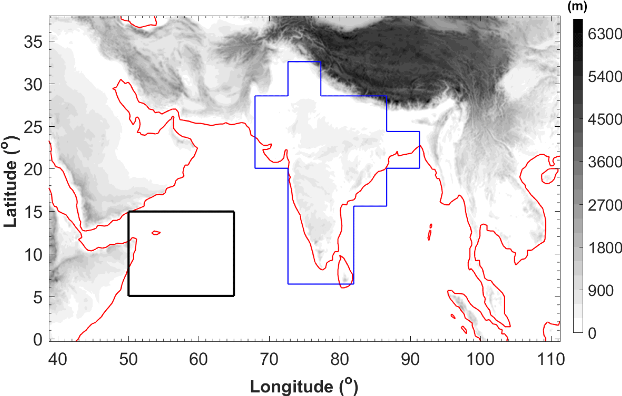
Figure 1Model domain used in the WRF simulations with topography (grayscale) and coastlines (red lines). The black box shows the climatic zone used for the calculation of KELLJ index and the blue polygon shows the Indian subcontinent.
Five boreal summers are simulated from 2007 to 2011 in this study. The 6-hourly ERA-Interim reanalysis (Dee et al., 2011) is used as the initial and boundary conditions for the simulations, and sea surface temperature (SST) is updated every 6 h using the ERA-Interim SST data. The ERA-Interim reanalysis is produced with a sequential data assimilation scheme, advancing forward in time using 12-hourly analysis cycles. The zonal and meridional winds in the reanalysis are directly assimilated from observational data; thus the large-scale monsoon circulation is well captured in the reanalysis. The Indian summer monsoon precipitation climatology in ERA-Interim has also been compared with that in other reanalysis data sets, and the results show that ERA-Interim has the highest skill to reproduce the Indian summer monsoon rainfall though obvious biases can still be found (Kishore et al., 2016; Lin et al., 2014). The model integrations start from 00:00 UTC, 20 April, in each year. For the first 3 days, a spectral nudging is applied to relax the horizontal wind with a meridional wave number of 0–2 and zonal wavenumber of 0–4, which constrains the large-scale flow and convergence in the domain and allows for the mesoscale to saturate in the spectral space (W15). The simulations are integrated until October 30 for each year in order to capture the withdrawal of the ISM in different years. The simulated spatial distributions and temporal variations of surface rainfall are verified against the 3-hourly 0.25∘ Tropical Rainfall Measurement Mission (TRMM) 3B42 rainfall product version 7A, while the large-scale circulations and atmospheric conditions in the simulations are verified against the ERA-interim reanalysis.
Besides the control simulations at the 9 km gray-zone resolution (WRF-gray hereafter), another set of numerical simulations with a coarser grid spacing (27 km, WRF-27km hereafter) are also conducted in this study to evaluate the extent to which the cloud-permitting simulations at gray-zone resolution can improve the simulation of the ISM and MISO. The configuration of the coarse simulations is similar to that of the WRF-gray configuration, except that a cumulus parameterization scheme is used to represent the subgrid-scale convective activity. Mukhopadhyay et al. (2010) investigated the impacts of different cumulus schemes on the systematic biases of ISM rainfall simulation in the WRF RCM. They compared the simulations conducted with three different convective schemes, namely the Grell–Devenyi (GD; Grell and Dévényi, 2002), the Betts–Miller–Janjić (BMJ; Janjić, 1994; Betts and Miller, 1986), and the Kain–Fritsch (KF; Kain, 2004) schemes. Results show that KF has a high moist bias while GD shows a high dry bias in simulating the monsoonal rainfall climatology. Among these three schemes, BMJ can produce the most reasonable monsoonal precipitation over the Indian subcontinent with the least bias. Similar results can also be found in Srinivas et al. (2013). Hence, the BMJ scheme has been used in the WRF-27km simulations.
Figure 2 shows the daily surface precipitation averaged over the Indian subcontinent (shown by the blue polygon in Fig. 1) from TRMM observation, WRF-gray, and WRF-27km during the monsoon seasons (JJAS). An apparent moist bias of surface precipitation can be found for all 5 years (2007 to 2011) in WRF-27km, while this systematic bias is reduced considerably in WRF-gray. One reason of the moist bias reduction is that topography is better resolved in WRF-gray than in WRF-27km (the spatial resolution of topography is 3 times higher in WRF-gray). Thus, local convective activity is better simulated, and the total surface precipitation is less over the Himalaya foothills and Western Ghats in WRF-gray (not shown here). Besides mountainous areas, surface rainfall simulation over the plains and oceanic regions also shows a high moist bias in WRF-27km, which improved dramatically in WRF-gray. These results show that higher model resolution and a better simulation of the large-scale atmospheric circulation contributes to the improvement of the monsoon rainfall simulation in WRF-gray, a finding that will be discussed in detail in the following sections. In addition, we also find that the simulations at gray-zone resolution (WRF-gray) can better capture the interannual variability of the monsoon rainfall amount than WRF-27km. The rest of this paper will focus on the assessment of the ISM and MISO simulations in WRF-gray, while both the MISO simulations in WRF-gray and WRF-27km will be compared to the observations in Sect. 4.
The large-scale atmospheric circulation and spatiotemporal patterns of the monsoon rainfall in WRF-gray are first assessed in this section. Figure 3a and b show the 5-year JJAS climatological mean 200 hPa winds and geopotential heights extracted from ERA-Interim and WRF-gray. During the summer monsoon, the upper troposphere (200 hPa) is characterized by a strong anti-cyclone over the Tibetan Plateau and easterly winds over the Indian subcontinent. The model captures well the wind and geopotential height patterns in the upper troposphere, though the Tibetan high pressure and easterly winds in WRF-gray are slightly stronger than in ERA-Interim (Fig. 3b). At lower levels (850 hPa), the model realistically simulates the geographical position and strength of the Somali Jet over the Arabian Sea, with a slight overestimation of the wind speed (Fig. 3c and d). Moisture is transported by the strong low-level winds from the Arabian Sea to the Indian subcontinent. As a result, a precipitable water maximum can be found over Western Ghats and the eastern coast of the Arabian Sea in both ERA-Interim and WRF-gray, though the precipitable water over the mountainous rages of Western Ghats in WRF-gray is slightly higher than that in ERA-Interim. In addition, WRF-gray also captures well the rain shadow downwind of the mountainous areas of central and southern India, where a slight dry bias can be noticed (Fig. 3d). The low-level southwesterly winds over the Bay of Bengal in WRF-gray are stronger than those in ERA-Interim, which leads to an overestimation in the precipitable water over the north tip of the Bay of Bengal, the west coast of Myanmar, and the foothills of Himalaya (Fig. 3d). A comparison of JJAS-averaged daily rainfall distribution observed by TRMM with that simulated by WRF-gray is shown in Fig. 3e and f. Overall, WRF-gray realistically captures the spatial pattern of the monsoon rainfall with the regional rainfall maximums over Western Ghats, central India, Himalaya foothills, and the west coast of Myanmar. Consistent with the biases shown in the low-level wind and precipitable water fields (Fig. 3d), the simulated surface rainfall shows a dry bias over central India and a moist bias over Western Ghats, Himalaya foothills, and the west coast of Myanmar (the Bay of Bengal). Similar features can also been found in earlier RCM studies (e.g., Lucas-Picher et al., 2011; Rockel and Geyer, 2008), which have shown that these biases can be explained by the way that surface schemes cannot well simulate the land–sea pressure and temperature contrasts that drive the monsoon dynamics and induce an overestimation of surface wind speed over oceans. This may explain an overestimation of the surface evaporation over the tropical oceans and excess precipitation downstream over the mountain ranges of Southeast Asia.

Figure 2Averaged daily rainfall over the Indian subcontinent for JJAS in different years from TRMM observation (blue bars), WRF-gray (green bars), and WRF-27km (yellow bars).
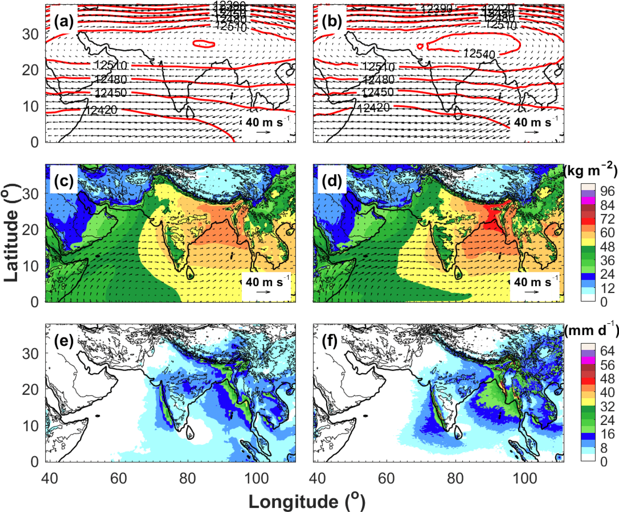
Figure 3Five-year mean monsoon (JJAS) winds (vectors) and geopotential heights (red contours) at 200 hPa from (a) ERA-Interim and (b) WRF-gray; winds (vectors) and precipitable water (color shadings) at 850 hPa from (c) ERA-Interim and (d) WRF-gray; daily surface precipitation (color shadings) from (e) TRMM and (f) WRF-gray. Topography is shown by the black contours starts at 500 m with a 1000 m interval.
The Somali Jet over the Arabian Sea is a central feature of the Indian summer monsoon. Its emergence is crucial in determining the onset precipitation over the Indian subcontinent (Ji and Vernekar, 1997; Joseph and Sijikumar, 2004). Ajayamohan (2007) proposed an index to represent the kinetic energy (KE) of the Somali Jet (KELLJ), which is defined as the mean KE of winds at 850 hPa averaged over 50–65∘ E and 5–15∘ N (shown by the black box in Fig. 1). The same index is applied here to assess the strength of the Somali Jet. The 5-year temporal evolutions of KELLJ calculated from WRF-gray and WRF-27km are compared with that calculated from ERA-Interim in Fig. 4. In general, the simulations well capture the evolution of KELLJ in different years. Sudden increases in KE of the Somali Jet in late May associated with the monsoon onsets are well reproduced in both WRF-gray and WRF-27km. The Somali Jet is stronger during the monsoon (JJAS) than in May and October, which leads to a stronger precipitation over the Indian subcontinent during the ISM. WRF-gray also well simulates the intraseasonal variation of KELLJ and the decrease in KE associated with the withdrawal of the monsoon in each year. Overall, the Somali Jet in WRF-gray is slightly stronger than that in ERA-Interim, which is similar to the above analysis in Fig. 3c and d. However, the strength of the Somali Jet in WRF-27km is much stronger when compared to WRF-gray and ERA-Interim. This is one of the reasons why there is a high moist bias of monsoon rainfall in WRF-27km. In general, the simulation at gray-zone resolution can better capture the large-scale atmospheric circulation of Indian summer monsoon than the coarser-resolution simulation with cumulus scheme.
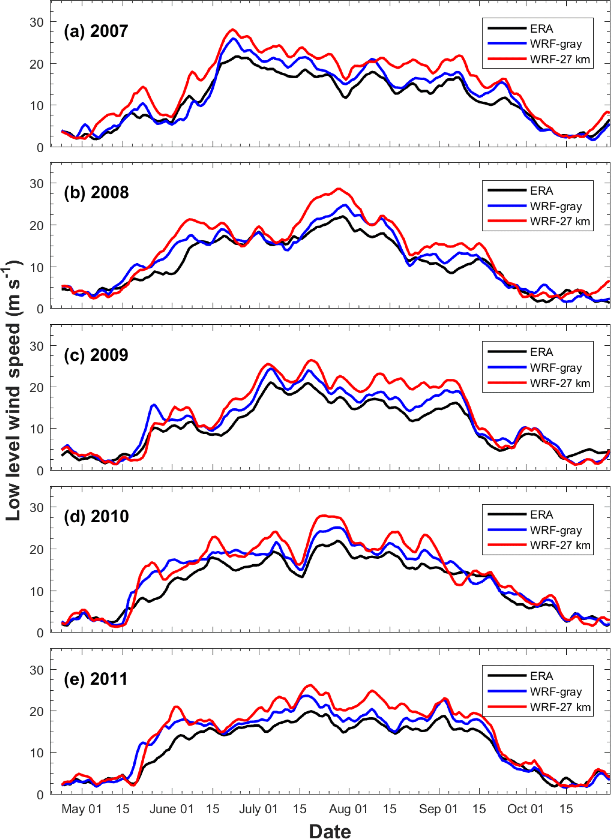
Figure 4Temporal evolution of KELLJ indices in (a) 2007, (b) 2008, (c) 2009, (d) 2010, and (e) 2011 from ERA-Interim (black lines), WRF-gray (blue lines), and WRF-27km (red lines). A 5-day moving average is applied to the time series.
The evolution of surface rainfall averaged over the Indian subcontinent (shown by the blue polygon) from WRF-gray and WRF-27km is compared with that from TRMM observations (Fig. 5). The seasonal mean Indian monsoon rainfall for each year in TRMM, WRF-gray, and WRF-27km has been given in each panel. Generally speaking, WRF-gray well captures the mean strength and intraseasonal variations of the monsoon rainfall. In these 5 years, the accumulated monsoonal rainfall amount over the Indian subcontinent is largest in 2010 (9.1 mm day−1) and smallest in 2009 (7.1 mm day−1). Year 2009 is also one of the driest years in the past 3 decades. Corresponding to the evolution of the Somali Jet, rainfall over the Indian subcontinent begins to increase from late May, reaches it maximum during JJAS, and decreases again in late September or early October, changes of which are associated with the onsets and withdrawals of the ISM. The onset and withdrawal of the ISM are well captured by WRF-gray in most years except that the onset of the 2007 ISM in WRF-gray is later than those in TRMM observations. The main reason for the 2007 ISM later onset in WRF-gray is that the super cyclonic storm Gonu, which induced strong precipitation over western India and had considerable influence over the onset of the 2007 ISM (Najar and Salvekar, 2010), was not well captured in the WRF simulation (the position of Gonu has a southwest shift in WRF-gray, not shown here). The ISM also shows a strong ISO in each year in the form of “active” and “break” spells of monsoon rainfall over the Indian subcontinent. These “active” and “break” phases of ISMs are closely related to the strengthening and weakening of the Somali Jet (Fig. 4). Despite the biases of the monsoon rainfall intensity, we find that WRF-gray well captures most “active” and “break” spells, which gives us further confidence that MISOs can be qualitatively simulated in the RCMs at gray-zone resolution. Compared to WRF-gray, the surface rainfall in WRF-27km shows a high moist bias over the Indian subcontinent, consistent with the overprediction of the Somali Jet strength shown in Fig. 4 and the analysis of seasonal mean rainfall in Fig. 2. Also, the intraseasonal variation of monsoon rainfall is more poorly simulated in WRF-27km than in WRF-gray. For example, the “active” and “break” spells from August to September in 2007 are well captured by WRF-gray while not simulated in WRF-27km. The 5-year averaged correlation coefficient of precipitation between WRF-gray (WRF-27km) and TRMM observations is 0.786 (0.714). These results show that the simulation at gray-zone resolution can better capture both the mean intensity and the intraseasonal variation of Indian summer monsoon than the coarser-resolution simulation using cumulus scheme.
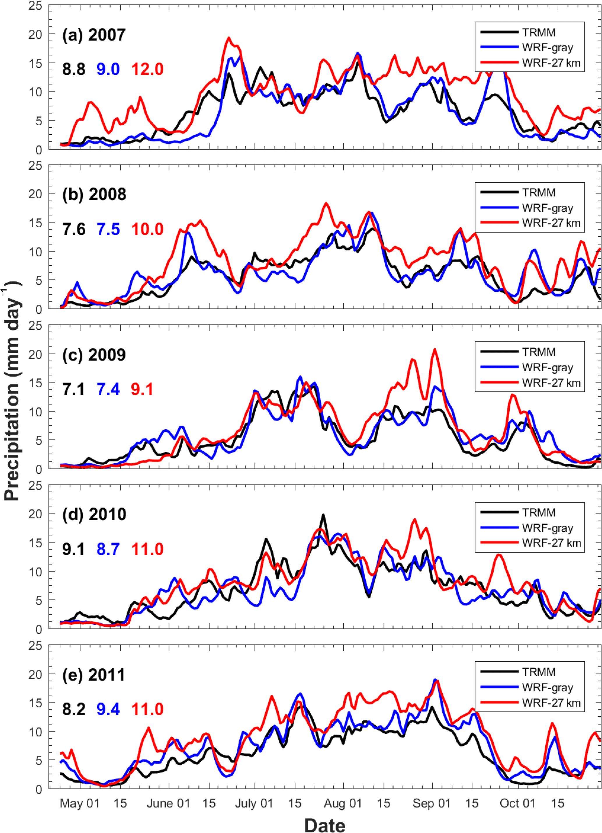
Figure 5Temporal evolution of daily surface rainfall averaged over the Indian subcontinent in (a) 2007, (b) 2008, (c) 2009, (d) 2010, and (e) 2011 from TRMM (black lines), WRF-gray (blue lines), and WRF-27km (red lines). A 5-day moving average is applied to the time series. The seasonal mean (June to September) of daily surface rainfall amounts averaged over the Indian subcontinent from TRMM (black), WRF-gray (blue), and WRF-27km (red) are also shown in the figure.
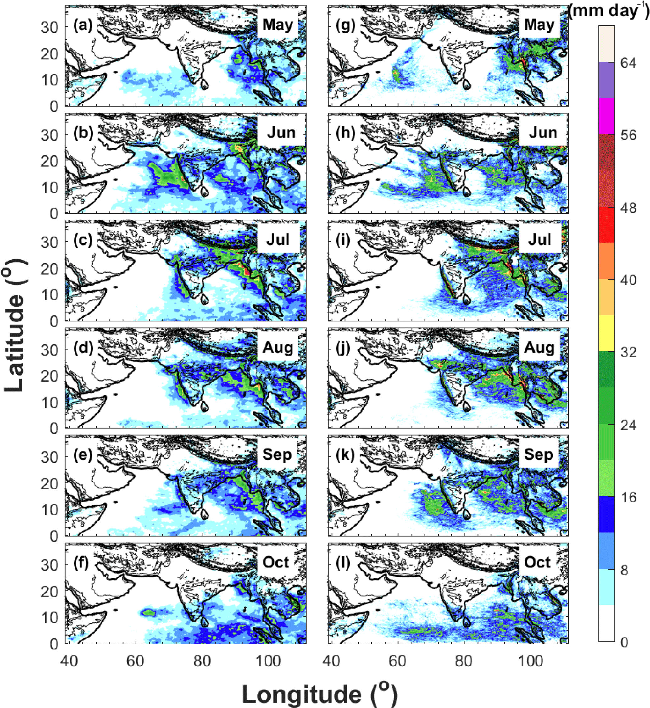
Figure 6Spatial distributions of averaged daily surface precipitation from May to October in year 2007 derived from (a–f) TRMM and (g–l) WRF-gray.
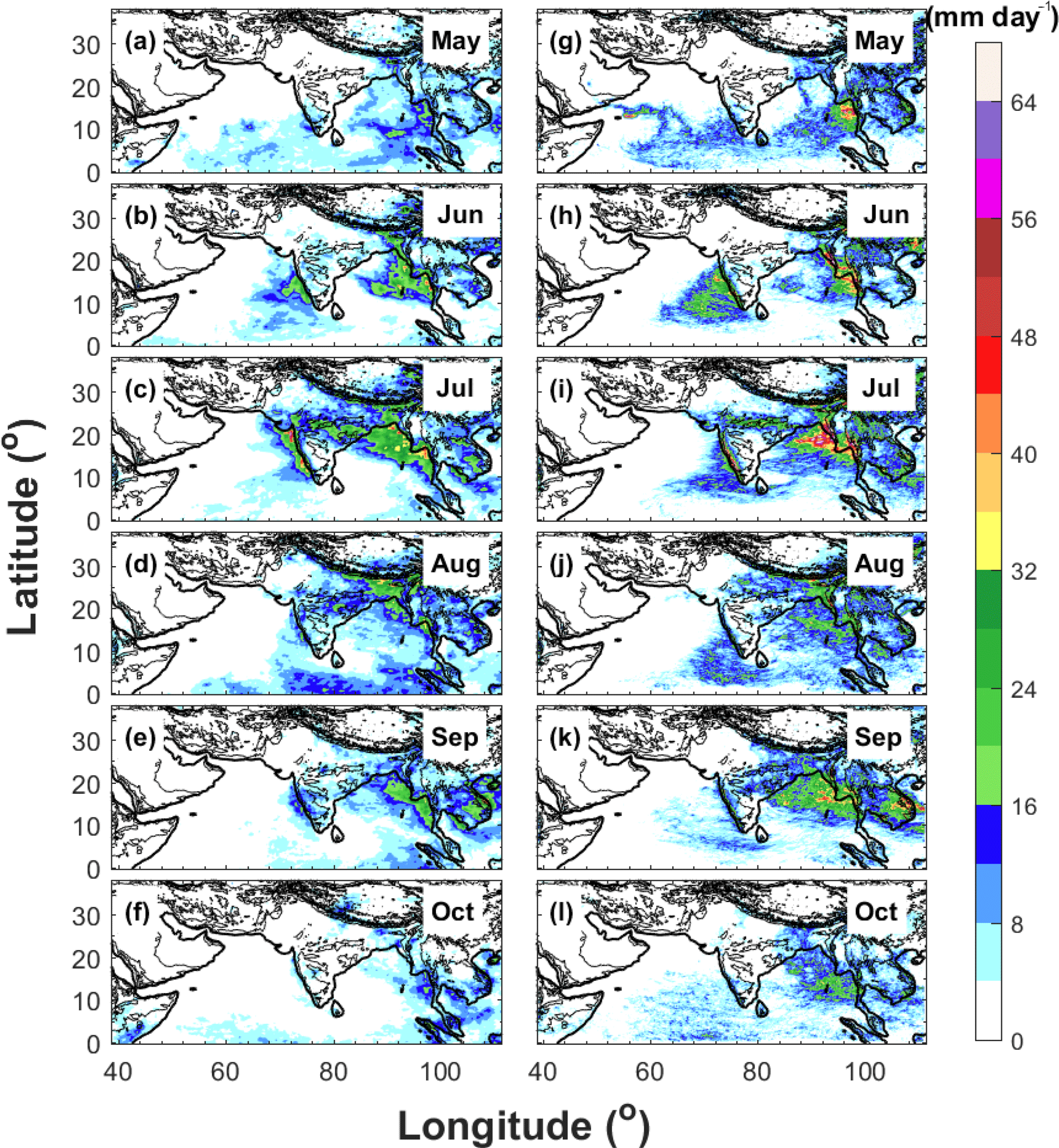
Figure 7Spatial distributions of averaged daily surface precipitation from May to October in year 2009 derived from (a–f) TRMM and (g–l) WRF-gray.
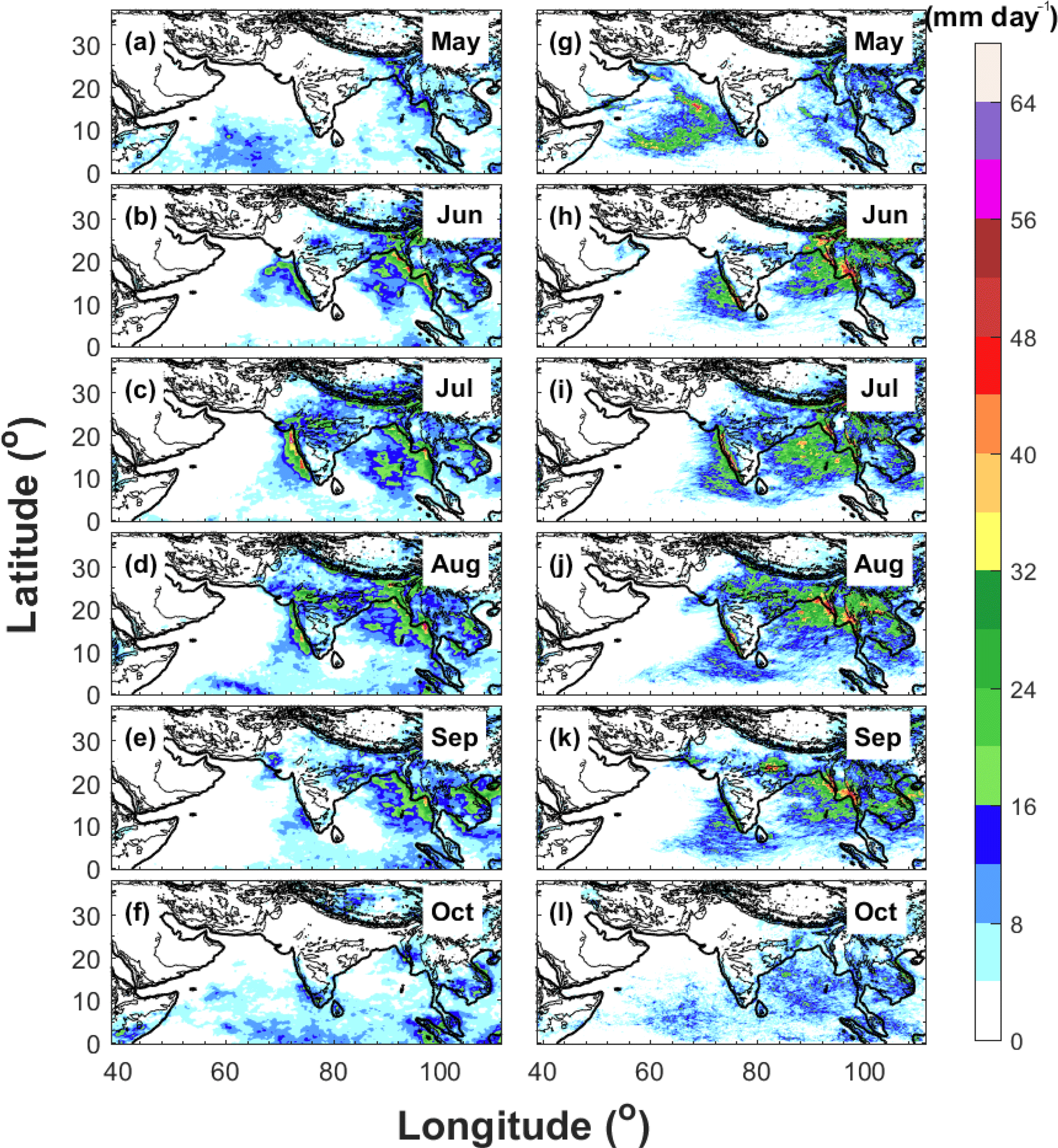
Figure 8Spatial distributions of averaged daily surface precipitation from May to October in year 2011 derived from (a–f) TRMM and (g–l) WRF-gray.
The spatial distributions of monthly mean precipitation from TRMM and WRF-gray in 2007, 2009, and 2011 are compared in Figs. 6–8. Similar to the analysis of Fig. 3, the model well captures the rainfall centers over Western Ghats, central India, Himalaya foothills, and the west coast of Myanmar during the summer monsoon seasons, with an overestimation of precipitation over the west coast of Myanmar and Himalaya foothills due to the overprediction of low-level wind over the Bay of Bengal. With high spatial resolution, WRF-gray is able to capture finer details of orographic precipitation over the mountainous rages (for example, along the west coastline of the Indian subcontinent). In addition, the interannual variability of monsoon rainfall is also well simulated in WRF-gray (Figs. 6–8). In 2007, rainfall is very weak over the Indian subcontinent in May though orographic precipitation can still be found over the mountainous ranges along the western coastlines (Fig. 6a and g). Accompanying the onset of the ISM and the enhancement of low-level winds over the Arabian Sea, precipitation over the west coast of the Indian subcontinent and its adjacent oceans increases dramatically in June (Fig. 6b and h). In July, the precipitation center along the west coast of the Indian subcontinent is still apparent and the precipitation over central India increases considerably (Fig. 6c and i). Rainfall over the Himalaya foothills and the west coast of Myanmar also reaches its strongest stage during this month. In August, rainfall over central India and the west coast of Myanmar are still strong while the precipitation near the Himalaya foothills decreases (Fig. 6d and j). The rainfall intensity over the entire monsoon region decreases continually in September (Fig. 6e and k) and the precipitation over the Indian subcontinent becomes very weak in October (Fig. 6f and l), which signals the end of the monsoon season. When compared to 2007, the ISM in 2009 is drier, especially over the Indian subcontinent (Fig. 7). The onset and withdrawal of the 2009 ISM over the Indian subcontinent are in June and September. The significant “break” spells of the 2009 ISM in June, August, and September are well captured by WRF-gray (Figs. 5c, 7h, j, and k). The evolution of monthly mean precipitation in 2011 (Fig. 8) is similar to that in 2007 (Fig. 6) with the rainfall over the central India reaching its strongest stage in August (Fig. 8d and j). In May 2011, an apparent moist bias of precipitation can be found over the Arabian Sea in WRF-gray, which is induced by the formation of a spurious tropical cyclone in the simulation. Generally speaking, WRF-gray is able to capture the spatiotemporal features of the ISM rainfall. Though apparent biases can still be found, the intensity and spatial pattern of monsoon rainfall in WRF-gray verify well against the observations, especially over the Indian subcontinent.
As mentioned in the Introduction, the MISO has fundamental influences on the seasonal mean, predictability, and interannual variability of the ISM. Hence, the simulation of the MISO is very important for the credibility of the model in simulating the ISM. The section evaluates the ability of WRF-gray in simulating the MISO. MISO-phase composites of the surface rainfall and large-scale flows from WRF-gray are compared with those from the observations.
4.1 Indices for the MISO
Using the nonlinear Laplacian spectral analysis (NLSA) technique (Giannakis and Majda, 2012a, b), Sabeerali et al. (2017) developed improved indices for real-time monitoring of the MISO. NLSA is a nonlinear data analysis technique that combines ideas from kernel methods for harmonic analysis, delay embedding of dynamical systems, and machine learning (Belkin and Niyogi, 2003; Packard et al., 1980; Sauer et al., 1991; Coifman and Lafon, 2006). Compared to the classical covariance-based approaches (for example Suhas et al., 2013; Krishnamurthy and Shukla, 2007), a key advantage of NLSA is that it is able to extract the spatiotemporal modes of variability spanning multiple timescales without requiring bandpass filtering or seasonal partitioning of the input data. Compared to the MISO indices based on the empirical orthogonal function (EEOF) and multichannel singular spectral analysis (MSSA), the NLSA-based MISO indices have improved timescale separation, higher memory, and higher predictability. The hindcasts of these indices using operational extended-range output show that NLSA-based MISO indices remain predictable out to ∼ 3 weeks while other indices only have ∼ 2 weeks of predictability. The MISO indices constructed by NLSA can better resolve the spatiotemporal characteristics of MISOs. For example, the NLSA-based MISO indices have better temporal-phase coherence while maintaining the isolating ability of MISOs from the broadband data set. It can better resolve the tilted structure of MISO convection and the associated atmospheric circulation pattern through phase composites and also explain more fractional variance over the ocean regions (Sabeerali et al., 2017).
In order to evaluate the MISO simulation in WRF-gray, the NLSA MISO indices are applied in this study to construct the phase composites of rainfall and atmospheric circulation from WRF-gray and the observations. Figure 9 shows the daily evolution of the MISO in each year monitored by the two-dimensional phase space diagram constructed from the NLSA MISO indices. All indices are extracted from the TRMM observations. The 2-D phase space of the NLSA MISO indices is divided into eight phases to represent different phases of the MISO. The significant MISO event is defined as the instantaneous MISO whose amplitude is greater than 1.5 (shown by the black circle in Fig. 9). From Fig. 9, we see that the MISO activity in 2007, 2008, and 2009 is much more significant than in 2010 and 2011. The accumulated monsoon rainfall amount over the Indian subcontinent is high in 2007 (8.8 mm day−1), which also features the strongest MISO activity (Fig. 9a). The following year, 2008, is also a moist year with strong MISO activity from the end of June to the end of September (Fig. 9b). In 2009 (Fig. 9c), a severe drought year, the MISO is weak during the early and late stages of the monsoon season (June and September), but stronger in the midst of the monsoon season (July and August). The amplitudes of the MISO indices in 2010 and 2011 are much smaller, while significant MISO events can still be found in most monsoon months (July, August, and September) in 2011 (Fig. 9e).

Figure 92-D phase space diagrams for the NLSA MISO indices in years: (a) 2007, (b) 2008, (c) 2009, (d) 2010, and (e) 2011. A counterclockwise propagation from Phase 1 represents MISO's northward propagation. The circle centered at the origin has radius equal to 1.5, which is the threshold for identification of significant MISO events.
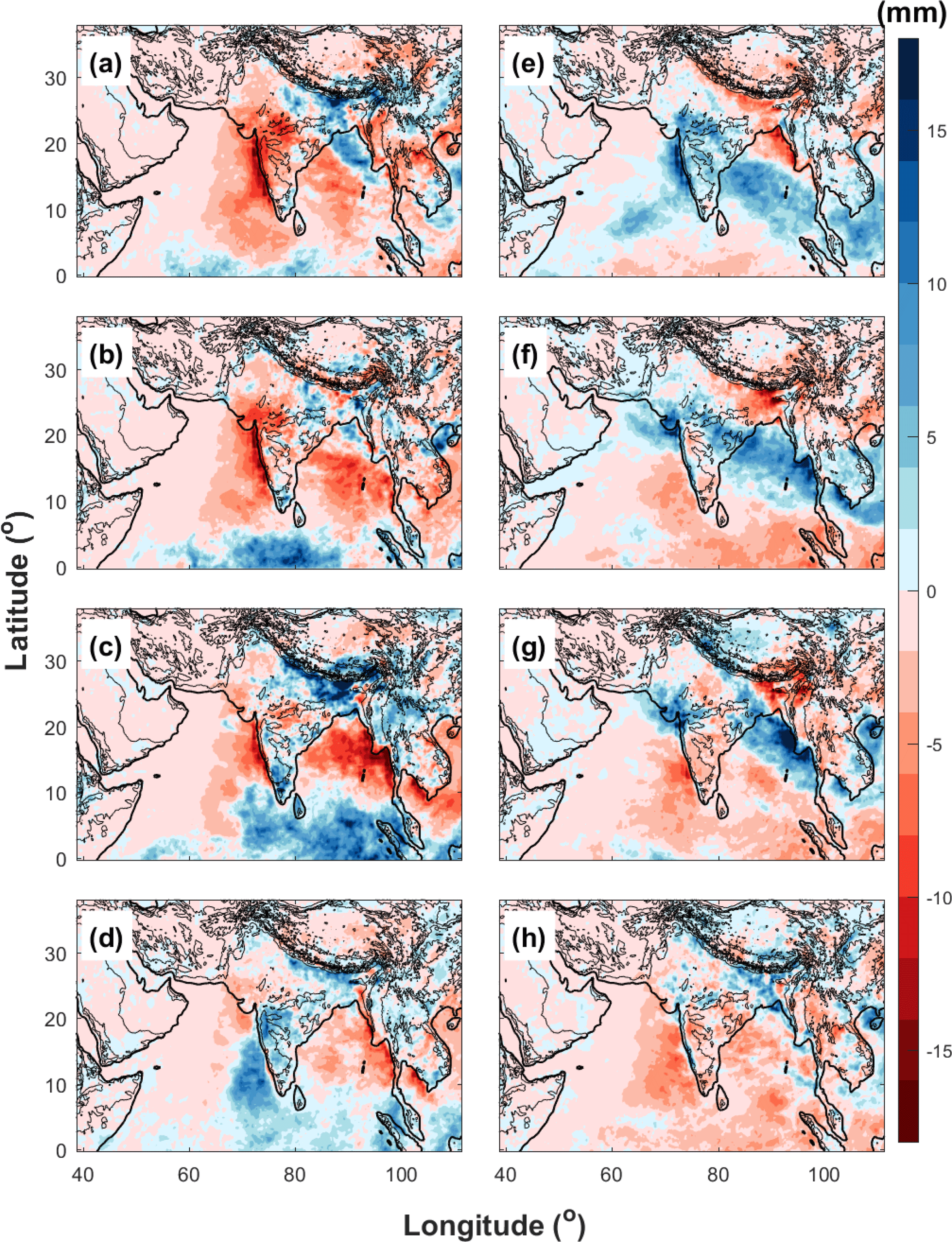
Figure 10Phase composites of daily surface rainfall anomalies obtained from TRMM (a–h: Phase 1 to 8).
4.2 Phase composites of surface rainfall
Figure 10 shows the phase composites of daily surface rainfall anomalies obtained from TRMM observations based on the NLSA MISO indices (the 5-year daily climatology is used to separate the anomalies). The phase composites are computed by averaging the significant MISO anomalies. An apparent northeastward propagation of the MISO can be found in the phase composites (from Phase 1 to Phase 8), which corresponds to the counterclockwise rotation in the 2-D phase space of the MISO indices (Fig. 9). Phase 1 shows the formation of enhanced rainfall anomalies over the tropic Indian Ocean (Fig. 10a). During this phase, rainfall over the Indian subcontinent is suppressed. The enhanced rainfall anomalies over the tropical ocean become stronger and move toward the Indian subcontinent in Phase 2 (Fig. 10b) and reach the Western Ghats and its adjoining oceans in Phase 3 and Phase 4 (Fig. 10c and d). In Phase 3, precipitation over the Indian subcontinent is enhanced while rainfall over the Bay of Bengal is suppressed (Fig. 10c). Rainfall over central India is enhanced considerably in Phase 4 (Fig. 10d) and forms a northwest–southeast enhanced rainfall line that stretches from the west coast of the Indian subcontinent to the south of Southeast Asia in Phase 5 (Fig. 10e). This enhanced rainfall line continually propagates to the northeast in Phase 6 (Fig. 10f). In Phase 7, the enhanced rainfall anomalies can still be found over northwest India and the west coast of Myanmar, while the rainfall in south India is suppressed by the MISO. The total rainfall over the entire basin is weakest during Phase 8, with the rainfall anomalies mostly negative over the inland regions of India (Fig. 10h). However, rainfall near Himalaya foothills begins to increase in this phase and reaches its maximum in Phase 1 (Fig. 10a). The phase composites of daily surface rainfall anomalies obtained from 5-year TRMM observations in this study are similar to the 26-year phase composites in Sabeerali et al. (2017), showing that the 5-year rainfall statistics reflect the climatological characteristics of the MISO.
Figure 11 presents the phase composites of daily surface rainfall anomalies obtained from WRF-gray. Despite differences in the intensity and location of rainfall anomalies, the MISO simulation in WRF-gray verified well against the TRMM observations. The fundamental features of rainfall anomalies in all eight phases of the MISO are well captured by WRF-gray: for example, the northeastward propagation of the enhanced rainfall anomalies, the “active” and “break” phases of the monsoon rainfall over the Indian subcontinent, the northwest–southeast enhanced rainfall line in Phases 5 and 6, the increase in rainfall over Himalaya foothills in Phases 8 and 1 and so on. Nonetheless, we also notice that the amplitude of the rainfall anomalies in WRF-gray is slightly larger than that in the TRMM observations, which reflects that the model-simulated MISO is stronger than that in the satellite observations.
In order to evaluate to what extent the RCM at gray-zone resolution can improve the simulation of the MISO, the phase composites of daily surface rainfall anomalies obtained from WRF-27km (Fig. 12) are also compared with those from the TRMM observations (Fig. 10) and WRF-gray (Fig. 11) in this section. We find that the amplitude of rainfall anomalies in WRF-27km is much larger than that in WRF-gray and TRMM observations, which shows the WRF-27km has larger systematic biases than WRF-gray in simulating the MISO intensity. Though WRF-27km can also basically capture the “active” (Fig. 12d–f) and “break” (Fig. 12h, a and b) phases of the ISM, it shows a larger bias in the spatiotemporal distributions of the rainfall anomalies during the different phases of the MISO than WRF-gray. For example, the rainfall anomalies in Phase 1 and 2 (Fig. 12a and b) are shifted northward, consistent with a faster development of the MISO cycle in the coarse-resolution model. The northwest–southeast enhanced rainfall line shown in TRMM observations and WRF-gray is not clear in WRF-27km. This is possibly due to deficiencies in how WRF-27km captures stratiform rainfall, which could create a bias toward more patchy, deep convective events. The increase in rainfall over Himalaya foothills from Phase 8 to Phase 1 has not been well simulated in WRF-27km. Generally speaking, WRF-gray better simulates the MISO than WRF-27km, both regarding intensity and the spatiotemporal evolution.

Figure 11Phase composites of daily surface rainfall anomalies obtained from WRF-gray (a–h: Phase 1 to 8).
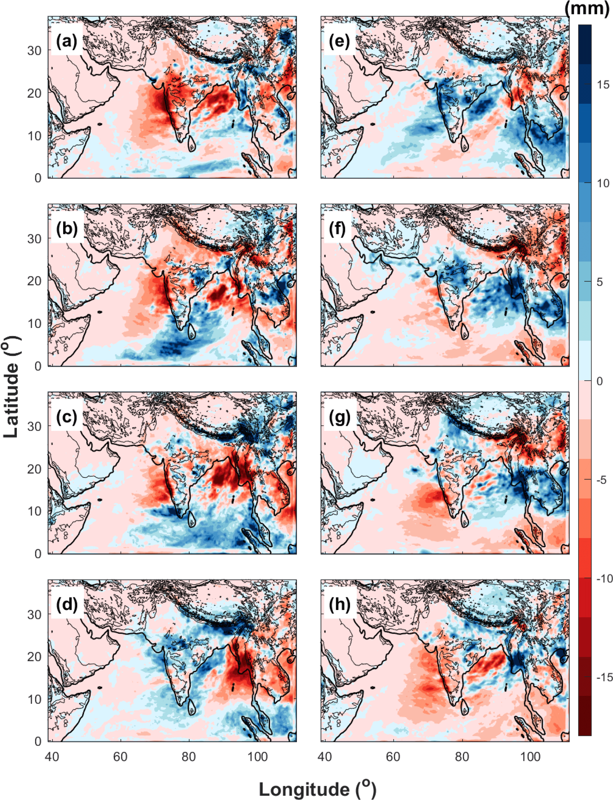
Figure 12Phase composites of daily surface rainfall anomalies obtained from WRF-27km (a–h: Phase 1 to 8).

Figure 13Spatial distributions of 10-day-averaged daily surface rainfall anomalies in (a, e) 1–10 July, (d, f) 11–20 July, (c, g) 21–31 July, and (d, h) 1–10 August, 2009 derived from TRMM (a, b, c, d) and WRF-gray (e, f, g, h).
Besides the phase composite, the evolution of 10-day-averaged daily surface rainfall anomalies in WRF-gray and TRMM observations are also compared with each other to further assess the credibility of WRF-gray in simulating the intraseasonal variability of the ISMs. The evolution of rainfall anomalies from 1 July to 10 August 2009 in TRMM observations and WRF-gray are shown in Fig. 13. During this period, the monsoon rainfall over the Indian subcontinent turns from a strong “active” phase to a strong “break” phase (Fig. 5c). The rainfall is enhanced over the west coast of the Indian subcontinent, central India, and the Bay of Bengal in the first 10 days of July (Fig. 13a), which is similar to the combined features of Phases 4 and 5 (Fig. 10d and e). The enhanced rainfall anomalies form a northwest–southeast line in mid-July (Fig. 13b), which corresponds to Phase 6. In the end of July, rainfall over most areas of the Indian subcontinent is suppressed, while the rainfall anomalies over northwest India and west coast of Myanmar are still positive (Fig. 13c). In early August, rainfall anomalies over the entire Indian subcontinent turn negative while rainfall over Himalaya foothills is enhanced (Fig. 13d), which is similar to the combined features of Phases 8 and 1 (Fig. 10h and a). Though small biases can be found in the simulated rainfall intensity and location, the 10-day evolutions of daily rainfall anomalies in WRF-gray verify well against the TRMM observations (Fig. 13e–h), which again proves that the cloud-permitting RCM at gray-zone resolution is credible in simulating the MISO.
4.3 Phase composites of atmospheric circulation
During the different phases of the MISO, the large-scale flows and atmospheric conditions also exhibit different behaviors (Raju et al., 2015; Goswami et al., 2003; Mukhopadhyay et al., 2010). Figure 14 shows the phase composites of the 850 hPa wind and precipitable water anomalies obtained from ERA-Interim. Consistent with the phase evolution of the enhanced daily rainfall anomalies (Fig. 10), the precipitable water anomalies also show an apparent northeastward propagation from Phase 1 (Fig. 14a) to Phase 8 (Fig. 14h), which corresponds to the counterclockwise rotation in the 2-D phase space of the MISO indices (Fig. 9). The major features of the MISO active phase (Fig. 14f) are the formation of low-pressure anomalies over northwest and central India which is associated with the southward shifting of monsoon trough (Raju et al., 2015). As a result, the strong westerly wind over the Arabian Sea and the Bay of Bengal also enhanced dramatically during the active phase of the MISO, transporting more water vapor from the oceans to the inland regions, leading to enhanced precipitable water anomalies over the land. The strength of the Somali Jet is also enhanced during the MISO active phase (Fig. 14f). During the break phase of the MISO, on the other hand, high-pressure anomalies can be found over northwest and central India, which is associated with the northward shifting of the monsoon trough. The westerly wind over the Arabian Sea and the Somali Jet are weakened during the break phase (Fig. 14a), which leads to the negative precipitable water and surface rainfall anomalies over the Indian subcontinent. Figure 15 shows the phase composites of 850 hPa wind anomalies and precipitable water anomalies obtained from WRF-gray. We find that WRF-gray well produces the large-scale features and precipitable water anomalies in different phases of the MISO (Fig. 15), which shows that the cloud-permitting RCM at gray-zone resolution can also well capture the large-scale circulation patterns of the MISO. We should note that, as with the rainfall anomalies shown in Fig. 11, the amplitudes of low-level wind and precipitable water anomalies in WRF-gray (Fig. 15) are larger than those in ERA-Interim (Fig. 14), which implies that the simulated MISO in WRF-gray is stronger than observations.

Figure 14Phase composites of 850 hPa wind and precipitable water anomalies obtained from ERA-Interim (a–h: Phase 1 to 8).

Figure 15Phase composites of 850 hPa wind and precipitable water anomalies obtained from WRF-gray (a–h: Phase 1 to 8).
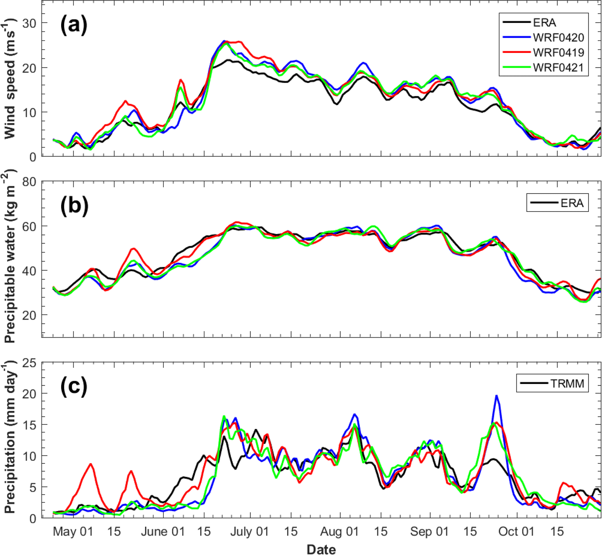
Figure 16Temporal evolutions of (a) KELLF indices, (b) precipitable water averaged over the Indian subcontinent, and (c) daily surface precipitation averaged over the Indian subcontinent in year 2007 from ERA-Interim/TRMM (black lines), WRF-gray simulation starts from 20 April (blue lines, control run), WRF-gray simulation starts from 19 April (red lines), and WRF-gray simulation starts from 21 April (green lines).
4.4 Sensitivity to initial dates
While WRF-gray captures many aspects of the ISM and MISO qualitatively, quantitative model biases are still apparent. These biases may have various causes such as the choice of surface scheme, the model domain size, and the initial conditions which the dynamical systems are highly sensitive to. The sensitivity of the WRF-gray simulation to initial dates is further investigated in this section. Figure 16 shows the temporal evolutions of the Somali Jet Strength (Fig. 16a), precipitation water (Fig. 16b), and precipitation (Fig. 16c) averaged over the Indian subcontinent in the WRF simulations at gray-zone resolution started on three different days (WRF0420: blue lines, started 00:00 UTC, 20 April; WRF0419: red lines, started 00:00 UTC, 19 April; WRF0421: green lines, started 00:00 UTC, 21 April) in 2007. Though all three WRF simulations are forced by the same lateral boundary conditions and the initial times are also close to each other, we can still find apparent differences in the simulated monsoon atmospheric circulation (Fig. 16a), humidity (Fig. 16b), and precipitation (Fig. 16c) among the three experiments. In particular, in May, there are apparent rainfall biases in WRF0419. However the onset of the ISM is better captured by WRF0419 than WRF0420 and WRF0421. The overprediction of monsoon rainfall from 15 September to 1 October in WRF0420 is considerably reduced in WRF0419 and WRF0421. Results show that the ISM and MISO simulations in RCM at gray-zone resolution are sensitive to the initial conditions.
Simulations of the ISM by cloud-permitting WRF model at gray resolution (9 km) are evaluated in this study, with a particular emphasis on the credibility of the MISO simulation. The model is forced by the ERA-Interim reanalysis for every year from 20 April to 30 October during 2007–2011. The model domain covers the entire Indian monsoon region which allows for the systematic evolution of the ISM internal dynamics. Compared with the RCM at a coarser resolution and using the cumulus parameterization scheme (WRF-27km), the systematic biases of monsoon rainfall climatology in the cloud-permitting RCM at gray-zone resolution (WRF-gray) are reduced considerably. The interannual variability of the accumulated monsoon rainfall over the Indian subcontinent is also better captured in WRF-gray.
Results from WRF-gray are compared quantitatively with the reanalysis and long-term TRMM observations. In general, WRF-gray could reproduce the fundamental features of ISM reasonably well. The Tibetan high pressure and easterly winds at 200 hPa in WRF-gray are slightly stronger than those in ERA-Interim. The low-level southwesterly winds over the Bay of Bengal in WRF-gray are also stronger when compared to that in the reanalysis, which leads to an overestimation of precipitable water and surface rainfall over the west coast of Myanmar and Himalaya foothills in WRF-gray. The temporal evolutions of the Somali Jet and surface rainfall averaged over the Indian subcontinent are also well simulated in WRF-gray. The model captures most onsets, breaks, and withdrawals of the ISMs, while the ISM onset in 2007 is later in WRF-gray than that in TRMM observations. Spatial distributions of monthly mean precipitation from TRMM and WRF-gray are further compared in the current study. Results show that WRF-gray could reproduce the spatial patterns of the monthly rainfall in each year and well capture the monsoon rainfall centers over Western Ghats, central India, Himalaya foothills, and the west coast of Myanmar. However, biases of rainfall intensity and position can still be found in WRF-gray.
Because the MISO has fundamental influences on the simulation and prediction of the ISM, the skill of WRF-gray in simulating the MISO is quantitatively assessed in this study. The NLSA MISO indices developed by Sabeerali et al. (2017) are applied in this study to construct the MISO-phase composites of surface rainfall and atmospheric circulations from WRF-gray and observations. The enhanced rainfall anomalies show a clear northeastward propagation from the MISO Phases 1 to 8. WRF-gray well captures the northeastward propagation and also simulates the spatial distribution of rainfall anomalies during different phases of the MISO. The low-level westerly wind over the Arabian Sea and the Somali Jet are strengthened (weakened) during the active (break) phase of the MISO, which induces higher (lower) precipitable water and stronger (weaker) precipitation over the Indian subcontinent. These features can also be well reproduced in WRF-gray, though the amplitude of rainfall, precipitable water, and wind anomalies in WRF-gray are larger than those in observations. When compared with WRF-27km, the systematic biases in simulating the MISO have been reduced considerably in WRF-gray, which shows that the cloud-permitting RCM is able to improve the simulations of the MISO associated with the ISM.
While WRF-gray captures many aspects of the ISM and MISO qualitatively, quantitative model biases are still apparent. The ISM simulation at gray-zone resolution is also sensitive to its initial conditions. Future studies should include more comprehensive investigation of the predictability of the ISO and MISO in RCM at gray-zone resolution.
TRMM precipitation data were obtained from the NASA Goddard Space Flight Center. ECMWF reanalysis data were retrieved from the ECMWF Public Datasets web interface (http://apps.ecmwf.int/datasets/). WRF output can be obtained upon request to xzc55@psu.edu.
The authors declare that they have no conflict of interest.
Many thanks to Ajaya Ravindran and Sabeerali Cherumadanakadan Thelliyil for
the multiple discussions that benefited this study. The authors Xingchao Chen
and Olivier Pauluis are supported by the New York University in Abu Dhabi
Research Institute under grant G1102. Fuqing Zhang is partially supported by
NSF grant AGS-1305798. The computations were carried out on the high-performance computing resources at NYUAD.
Edited by: Rolf Müller
Reviewed by: Shuguang Wang and David Straus
Ajayamohan, R. S.: Simulation of South-Asian Summer Monsoon in a GCM, Pure Appl. Geophys., 164, 2117–2140, https://doi.org/10.1007/s00024-007-0249-9, 2007.
Ajayamohan, R. S. and Goswami, B. N.: Potential predictability of the Asian summer monsoon on monthly and seasonal time scales, Meteorol. Atmos. Phys., 84, 83–100, https://doi.org/10.1007/s00703-002-0576-4, 2003.
Ajayamohan, R. S., Khouider, B., and Majda, A. J.: Simulation of monsoon intraseasonal oscillations in a coarse-resolution aquaplanet GCM, Geophys. Res. Lett., 41, 5662–5669, https://doi.org/10.1002/2014GL060662, 2014.
Belkin, M. and Niyogi, P.: Laplacian Eigenmaps for dimensionality reduction and data representation, Neural Comput., 15, 1373–1396, https://doi.org/10.1162/089976603321780317, 2003.
Betts, A. K. and Miller, M. J.: A new convective adjustment scheme. Part II: Single column tests using GATE wave, BOMEX, ATEX and arctic air-mass data sets, Q. J. Roy. Meteorol. Soc., 112, 693–709, https://doi.org/10.1002/qj.49711247308, 1986.
Bhaskaran, B., Mitchell, J. F. B., Lavery, J. R., and Lal, M.: Climatic response of the Indian subcontinent to doubled CO2 concentrations, Int. J. Climatol., 15, 873–892, https://doi.org/10.1002/joc.3370150804, 1995.
Bhaskaran, B., Jones, R. G., Murphy, J. M., and Noguer, M.: Simulations of the Indian summer monsoon using a nested regional climate model: domain size experiments, Clim. Dynam., 12, 573–587, https://doi.org/10.1007/bf00216267, 1996.
Bhaskaran, B., Murphy, J. M., and Jones, R. G.: Intraseasonal Oscillation in the Indian Summer Monsoon Simulated by Global and Nested Regional Climate Models, Mon. Weather Rev., 126, 3124–3134, https://doi.org/10.1175/1520-0493(1998)126<3124:ioitis>2.0.co;2, 1998.
Bollasina, M. A.: Hydrology: Probing the monsoon pulse, Nat. Clim. Change, 4, 422–423, https://doi.org/10.1038/nclimate2243, 2014.
Bryan, G. H., Wyngaard, J. C., and Fritsch, J. M.: Resolution Requirements for the Simulation of Deep Moist Convection, Mon. Weather Rev., 131, 2394–2416, https://doi.org/10.1175/1520-0493(2003)131<2394:rrftso>2.0.co;2, 2003.
Chatterjee, P. and Goswami, B. N.: Structure, genesis and scale selection of the tropical quasi-biweekly mode, Q. J. Roy. Meteorol. Soc., 130, 1171–1194, https://doi.org/10.1256/qj.03.133, 2004.
Chen, F. and Dudhia, J.: Coupling an Advanced Land Surface–Hydrology Model with the Penn State-NCAR MM5 Modeling System. Part I: Model Implementation and Sensitivity, Mon. Weather Rev., 129, 569–585, https://doi.org/10.1175/1520-0493(2001)129<0569:caalsh>2.0.co;2, 2001.
Chen, G.-S., Liu, Z., Clemens, S. C., Prell, W. L., and Liu, X.: Modeling the time-dependent response of the Asian summer monsoon to obliquity forcing in a coupled GCM: a PHASEMAP sensitivity experiment, Climate Dynam., 36, 695-710, 10.1007/s00382-010-0740-3, 2011.
Coifman, R. R. and Lafon, S.: Diffusion maps, Appl. Comput. Harmon. Anal., 21, 5–30, https://doi.org/10.1016/j.acha.2006.04.006, 2006.
Das, S., Mitra, A. K., Iyengar, G. R., and Mohandas, S.: Comprehensive test of different cumulus parameterization schemes for the simulation of the Indian summer monsoon, Meteorol. Atmos. Phys., 78, 227–244, https://doi.org/10.1007/s703-001-8176-1, 2001.
Dash, S. K., Shekhar, M. S., and Singh, G. P.: Simulation of Indian summer monsoon circulation and rainfall using RegCM3, Theor. Appl. Climatol., 86, 161–172, https://doi.org/10.1007/s00704-006-0204-1, 2006.
Dee, D. P., Uppala, S. M., Simmons, A. J., Berrisford, P., Poli, P., Kobayashi, S., Andrae, U., Balmaseda, M. A., Balsamo, G., Bauer, P., Bechtold, P., Beljaars, A. C. M., van de Berg, L., Bidlot, J., Bormann, N., Delsol, C., Dragani, R., Fuentes, M., Geer, A. J., Haimberger, L., Healy, S. B., Hersbach, H., Hólm, E. V., Isaksen, L., Kållberg, P., Köhler, M., Matricardi, M., McNally, A. P., Monge-Sanz, B. M., Morcrette, J. J., Park, B. K., Peubey, C., de Rosnay, P., Tavolato, C., Thépaut, J. N., and Vitart, F.: The ERA-Interim reanalysis: configuration and performance of the data assimilation system, Q. J. Roy. Meteorol. Soc., 137, 553–597, https://doi.org/10.1002/qj.828, 2011.
Giannakis, D. and Majda, A. J.: Nonlinear Laplacian spectral analysis for time series with intermittency and low-frequency variability, P. Natl. Acad. Sci. USA, 109, 2222–2227, https://doi.org/10.1073/pnas.1118984109, 2012a.
Giannakis, D. and Majda, A. J.: Comparing low-frequency and intermittent variability in comprehensive climate models through nonlinear Laplacian spectral analysis, Geophys. Res. Lett., 39, L10710, https://doi.org/10.1029/2012GL051575, 2012b.
Giorgi, F.: Regional climate modeling: Status and perspectives, J. Phys. IV France, 139, 101–118, 2006.
Goswami, B. N.: Dynamical predictability of seasonal monsoon rainfall: Problems and prospects, Proc. Indian Nat. Sci. Acad. Pt. A, 60, 101–101, 1994.
Goswami, B. B. and Goswami, B. N.: A road map for improving dry-bias in simulating the South Asian monsoon precipitation by climate models, Clim. Dynam., 49, 2025, https://doi.org/10.1007/s00382-016-3439-2, 2016.
Goswami, B. N. and Ajayamohan, R. S.: Intraseasonal Oscillations and Interannual Variability of the Indian Summer Monsoon, J. Climate, 14, 1180–1198, https://doi.org/10.1175/1520-0442(2001)014<1180:ioaivo>2.0.co;2, 2001.
Goswami, B. N., Ajayamohan, R. S., Xavier, P. K., and Sengupta, D.: Clustering of synoptic activity by Indian summer monsoon intraseasonal oscillations, Geophys. Res. Lett., 30, 1431, https://doi.org/10.1029/2002GL016734, 2003.
Grell, G. A. and Dévényi, D.: A generalized approach to parameterizing convection combining ensemble and data assimilation techniques, Geophys. Res. Lett., 29, 38-31–38-34, https://doi.org/10.1029/2002GL015311, 2002.
Hong, S.-Y., Noh, Y., and Dudhia, J.: A New Vertical Diffusion Package with an Explicit Treatment of Entrainment Processes, Mon. Weather Rev., 134, 2318–2341, https://doi.org/10.1175/mwr3199.1, 2006.
Hu, X.-M., Nielsen-Gammon, J. W., and Zhang, F.: Evaluation of Three Planetary Boundary Layer Schemes in the WRF Model, J. Appl. Meteorol. Clim., 49, 1831-01844, https://doi.org/10.1175/2010jamc2432.1, 2010.
Iacono, M. J., Delamere, J. S., Mlawer, E. J., Shephard, M. W., Clough, S. A., and Collins, W. D.: Radiative forcing by long-lived greenhouse gases: Calculations with the AER radiative transfer models, J. Geophys. Res.-Atmos., 113, D13103, https://doi.org/10.1029/2008JD009944, 2008.
Jain, S. K. and Kumar, V.: Trend analysis of rainfall and temperature data for India, Current Science (Bangalore), 102, 37–49, 2012.
Janjić, Z. I.: The Step-Mountain Eta Coordinate Model: Further Developments of the Convection, Viscous Sublayer, and Turbulence Closure Schemes, Mon. WeatherRev., 122, 927–945, https://doi.org/10.1175/1520-0493(1994)122<0927:tsmecm>2.0.co;2, 1994.
Ji, Y. and Vernekar, A. D.: Simulation of the Asian Summer Monsoons of 1987 and 1988 with a Regional Model Nested in a Global GCM, J. Climate, 10, 1965–1979, https://doi.org/10.1175/1520-0442(1997)010<1965:sotasm>2.0.co;2, 1997.
Jiang, X., Li, T., and Wang, B.: Structures and Mechanisms of the Northward Propagating Boreal Summer Intraseasonal Oscillation, J. Climate, 17, 1022–1039, https://doi.org/10.1175/1520-0442(2004)017<1022:samotn>2.0.co;2, 2004.
Joseph, P. V. and Sijikumar, S.: Intraseasonal Variability of the Low-Level Jet Stream of the Asian Summer Monsoon, J. Climate, 17, 1449–1458, https://doi.org/10.1175/1520-0442(2004)017<1449:ivotlj>2.0.co;2, 2004.
Kain, J. S.: The Kain–Fritsch Convective Parameterization: An Update, J. Appl. Meteorol., 43, 170-181, 10.1175/1520-0450(2004)043<0170:tkcpau>2.0.co;2, 2004.
Kikuchi, K., Wang, B., and Kajikawa, Y.: Bimodal representation of the tropical intraseasonal oscillation, Clim. Dynam., 38, 1989–2000, https://doi.org/10.1007/s00382-011-1159-1, 2012.
Kishore, P., Jyothi, S., Basha, G., Rao, S. V. B., Rajeevan, M., Velicogna, I., and Sutterley, T. C.: Precipitation climatology over India: validation with observations and reanalysis datasets and spatial trends, Clim. Dynam., 46, 541–556, https://doi.org/10.1007/s00382-015-2597-y, 2016.
Klemp, J. B., Dudhia, J., and Hassiotis, A. D.: An Upper Gravity-Wave Absorbing Layer for NWP Applications, Mon. Weather Rev., 136, 3987–4004, https://doi.org/10.1175/2008mwr2596.1, 2008.
Kolusu, S., Prasanna, V., and Preethi, B.: Simulation of Indian summer monsoon intra-seasonal oscillations using WRF regional atmospheric model, Int. J. Earth Atmos. Sci., 1, 35–53, 2014.
Krishnamurthy, V. and Shukla, J.: Intraseasonal and Seasonally Persisting Patterns of Indian Monsoon Rainfall, J. Climate, 20, 3–20, https://doi.org/10.1175/jcli3981.1, 2007.
Krishnamurti, T. N. and Bhalme, H. N.: Oscillations of a Monsoon System. Part I. Observational Aspects, J. Atmos. Sci., 33, 1937–1954, https://doi.org/10.1175/1520-0469(1976)033<1937:ooamsp>2.0.co;2, 1976.
Lau, N.-C. and Ploshay, J. J.: Simulation of Synoptic- and Subsynoptic-Scale Phenomena Associated with the East Asian Summer Monsoon Using a High-Resolution GCM, Mon. Weather Rev., 137, 137–160, https://doi.org/10.1175/2008mwr2511.1, 2009.
Lau, W. K.-M. and Waliser, D. E.: Intraseasonal variability in the atmosphere-ocean climate system, Springer Science & Business Media, Berlin, 2011.
Lee, J.-Y., Wang, B., Wheeler, M. C., Fu, X., Waliser, D. E., and Kang, I.-S.: Real-time multivariate indices for the boreal summer intraseasonal oscillation over the Asian summer monsoon region, Clim. Dynam., 40, 493–509, https://doi.org/10.1007/s00382-012-1544-4, 2013.
Lim, K.-S. S. and Hong, S.-Y.: Development of an Effective Double-Moment Cloud Microphysics Scheme with Prognostic Cloud Condensation Nuclei (CCN) for Weather a nd Climate Models, Mon. Weather Rev., 138, 1587–1612, https://doi.org/10.1175/2009mwr2968.1, 2010.
Lin, R., Zhou, T., and Qian, Y.: Evaluation of Global Monsoon Precipitation Changes based on Five Reanalysis Datasets, J. Climate, 27, 1271–1289, https://doi.org/10.1175/jcli-d-13-00215.1, 2014.
Lucas-Picher, P., Christensen, J. H., Saeed, F., Kumar, P., Asharaf, S., Ahrens, B., Wiltshire, A. J., Jacob, D., and Hagemann, S.: Can regional climate models represent the Indian monsoon?, J. Hydrometeorol., 12, 849–868, 2011.
Mukhopadhyay, P., Taraphdar, S., Goswami, B., and Krishnakumar, K.: Indian summer monsoon precipitation climatology in a high-resolution regional climate model: Impacts of convective parameterization on systematic biases, Weather Forecast., 25, 369–387, 2010.
Najar, K. A. A. and Salvekar, P. S.: Understanding the Tropical Cyclone Gonu, in: Indian Ocean Tropical Cyclones and Climate Change, edited by: Charabi, Y., Springer Netherlands, Dordrecht, 359–369, 2010.
Oouchi, K., Noda, A. T., Satoh, M., Wang, B., Xie, S.-P., Takahashi, H. G., and Yasunari, T.: Asian summer monsoon simulated by a global cloud-system-resolving model: Diurnal to intra-seasonal variability, Geophys. Res. Lett., 36, L11815, https://doi.org/10.1029/2009GL038271, 2009.
Packard, N. H., Crutchfield, J. P., Farmer, J. D., and Shaw, R. S.: Geometry from a Time Series, Phys. Rev. Lett., 45, 712–716, 1980.
Pauluis, O. and Garner, S.: Sensitivity of Radiative–Convective Equilibrium Simulations to Horizontal Resolution, J. Atmos. Sci., 63, 1910–1923, https://doi.org/10.1175/jas3705.1, 2006.
Pleim, J. E.: A Combined Local and Nonlocal Closure Model for the Atmospheric Boundary Layer. Part I: Model Description and Testing, J. Appl. Meteorol. Clim., 46, 1383–1395, https://doi.org/10.1175/jam2539.1, 2007.
Prein, A. F., Langhans, W., Fosser, G., Ferrone, A., Ban, N., Goergen, K., Keller, M., Tölle, M., Gutjahr, O., Feser, F., Brisson, E., Kollet, S., Schmidli, J., van Lipzig, N. P. M., and Leung, R.: A review on regional convection-permitting climate modeling: Demonstrations, prospects, and challenges, Rev. Geophys., 53, 323–361, https://doi.org/10.1002/2014RG000475, 2015.
Rajendran, K. and Kitoh, A.: Indian summer monsoon in future climate projection by a super high-resolution global model, Current Science, 95, 1560–1569, 2008.
Raju, A., Parekh, A., Chowdary, J. S., and Gnanaseelan, C.: Assessment of the Indian summer monsoon in the WRF regional climate model, Clim. Dynam., 44, 3077–3100, https://doi.org/10.1007/s00382-014-2295-1, 2015.
Ramu, D. A., Sabeerali, C. T., Chattopadhyay, R., Rao, D. N., George, G., Dhakate, A. R., Salunke, K., Srivastava, A., and Rao, S. A.: Indian summer monsoon rainfall simulation and prediction skill in the CFSv2 coupled model: Impact of atmospheric horizontal resolution, J. Geophys. Res.-Atmos., 121, 2205–2221, https://doi.org/10.1002/2015JD024629, 2016.
Ratnam, J. V. and Kumar, K. K.: Sensitivity of the Simulated Monsoons of 1987 and 1988 to Convective Parameterization Schemes in MM5, J. Climate, 18, 2724–2743, https://doi.org/10.1175/jcli3390.1, 2005.
Rockel, B., and Geyer, B.: The performance of the regional climate model CLM in different climate regions, based on the example of precipitation, Meteorologische Zeitschrift, 17, 487-498, 2008.
Sabeerali, C. T., Rao, S. A., Ajayamohan, R. S., and Murtugudde, R.: On the relationship between Indian summer monsoon withdrawal and Indo-Pacific SST anomalies before and after 1976/1977 climate shift, Clim. Dynam., 39, 841–859, https://doi.org/10.1007/s00382-011-1269-9, 2012.
Sabeerali, C. T., Ajayamohan, R. S., Giannakis, D., and Majda, A. J.: Extraction and prediction of indices for monsoon intraseasonal oscillations: an approach based on nonlinear Laplacian spectral analysis, Clim. Dynam., 49, 3031, https://doi.org/10.1007/s00382-016-3491-y, 2017.
Saeed, F., Hagemann, S., and Jacob, D.: A framework for the evaluation of the South Asian summer monsoon in a regional climate model applied to REMO, Int. J. Climatol., 32, 430–440, https://doi.org/10.1002/joc.2285, 2012.
Samala, B. K. C., Banerjee, N., Kaginalkar, A., and Dalvi, M.: Study of the Indian summer monsoon using WRF–ROMS regional coupled model simulations, Atmos. Sci. Lett., 14, 20–27, https://doi.org/10.1002/asl2.409, 2013.
Sauer, T., Yorke, J. A., and Casdagli, M.: Embedology, Journal of Statistical Physics, 65, 579-616, 10.1007/bf01053745, 1991.
Shi, J. J., Tao, W.-K., Matsui, T., Cifelli, R., Hou, A., Lang, S., Tokay, A., Wang, N.-Y., Peters-Lidard, C., Skofronick-Jackson, G., Rutledge, S., and Petersen, W.: WRF Simulations of the 20–22 January 2007 Snow Events over Eastern Canada: Comparison with In Situ and Satellite Observations, J. Appl. Meteorol. Clim., 49, 2246–2266, https://doi.org/10.1175/2010jamc2282.1, 2010.
Sikka, D. R. and Gadgil, S.: On the Maximum Cloud Zone and the ITCZ over Indian, Longitudes during the Southwest Monsoon, Mon. Weather Rev., 108, 1840–1853, https://doi.org/10.1175/1520-0493(1980)108<1840:OTMCZA>2.0.CO;2, 1980.
Skamarock, W., Klemp, J., Dudhia, J., Gill, D., Barker, D., Duda, M., Huang, X., Wang, W., and Powers, J.: A Description of the Advanced Research WRF Version 3 (2008) NCAR Technical Note, NCAR, Boulder, CO, 2008.
Srinivas, C. V., Hariprasad, D., Bhaskar Rao, D. V., Anjaneyulu, Y., Baskaran, R., and Venkatraman, B.: Simulation of the Indian summer monsoon regional climate using advanced research WRF model, Int. J. Climatol., 33, 1195–1210, https://doi.org/10.1002/joc.3505, 2013.
Suhas, E., Neena, J. M., and Goswami, B. N.: An Indian monsoon intraseasonal oscillations (MISO) index for real time monitoring and forecast verification, Clim. Dynam., 40, 2605–2616, https://doi.org/10.1007/s00382-012-1462-5, 2013.
Vernekar, A. D. and Ji, Y.: Simulation of the Onset and Intraseasonal Variability of Two Contrasting Summer Monsoons, J. Climate, 12, 1707–1725, https://doi.org/10.1175/1520-0442(1999)012<1707:sotoai>2.0.co;2, 1999.
Wang, S., Sobel, A. H., Zhang, F., Sun, Y. Q., Yue, Y., and Zhou, L.: Regional Simulation of the October and November MJO Events Observed during the CINDY/DYNAMO Field Campaign at Gray Zone Resolution, J. Climate, 28, 2097–2119, https://doi.org/10.1175/jcli-d-14-00294.1, 2015.
Yasunari, T.: Structure of an Indian Summer Monsoon System with around 40-Day Period, J. Meteorol. Soc. Jpn. Ser. II, 59, 336–354, 1981.