the Creative Commons Attribution 3.0 License.
the Creative Commons Attribution 3.0 License.
Turbulent transport of energy across a forest and a semiarid shrubland
Peter Brugger
Frederik De Roo
Konstantin Kröniger
Dan Yakir
Eyal Rotenberg
Matthias Mauder
The role of secondary circulations has recently been studied in the context of well-defined surface heterogeneity in a semiarid ecosystem where it was found that energy balance closure over a desert–forest system and the structure of the boundary layer was impacted by advection and flux divergence. As a part of the CliFF (“Climate feedbacks and benefits of semi-arid forests”, a collaboration between KIT, Germany, and the Weizmann Institute, Israel) campaign, we studied the boundary layer dynamics and turbulent transport of energy corresponding to this effect in Yatir Forest situated in the Negev Desert in Israel. The forest surrounded by small shrubs presents a distinct feature of surface heterogeneity, allowing us to study the differences between their interactions with the atmosphere above by conducting measurements with two eddy covariance (EC) stations and two Doppler lidars. As expected, the turbulence intensity and vertical fluxes of momentum and sensible heat are found to be higher above the forest compared to the shrubland. Turbulent statistics indicative of nonlocal motions are also found to differ over the forest and shrubland and also display a strong diurnal cycle. The production of turbulent kinetic energy (TKE) over the forest is strongly mechanical, while buoyancy effects generate most of the TKE over the shrubland. Overall TKE production is much higher above the forest compared to the shrubland. The forest is also found to be more efficient in dissipating TKE. The TKE budget appears to be balanced on average both for the forest and shrubland, although the imbalance of the TKE budget, which includes the role of TKE transport, is found to be quite different in terms of diurnal cycles for the forest and shrubland. The difference in turbulent quantities and the relationships between the components of TKE budget are used to infer the characteristics of the turbulent transport of energy between the desert and the forest.
- Article
(10111 KB) - Full-text XML
- BibTeX
- EndNote


Understanding the interaction between vegetation canopies and atmosphere is a crucial component in the quantification of biosphere–atmosphere exchange of heat, carbon dioxide, water and trace gas fluxes. It is also important for the development of numerical weather and climate models where the fluxes in the canopy surface layer (CSL) and the atmospheric surface layer (ASL) are parameterized through bulk exchange coefficients of momentum and scalar. However, idealizations of the forest canopies as horizontally homogeneous momentum sinks and scalar sources introduces uncertainties in flux estimations and estimating diffusion coefficients. The presence of heterogeneities such as roughness transitions, complex topography and mesoscale circulations are common sources of such uncertainties that give rise to nonlocal motions and secondary circulations. These secondary circulations not only occur in forests but are also generic characteristics of boundary layer flows over natural and man-made landscapes with discongruity of land use types, surface moisture, temperature, etc. (Eder et al., 2015; Higgins et al., 2013). Different types of land cover such as agricultural lands or urban areas can affect local energy balance closure and the structure of the overlying boundary layer as well as cloud formation and regional weather (Eder et al., 2015; Fuentes et al., 2016). Strong differences in surface properties and large swaths of such surface patches are known to induce secondary circulations (Banerjee et al., 2013; Courault et al., 2007; Dalu and Pielke, 1993; Dixon et al., 2013; Garcia-Carreras et al., 2010; Kang and Lenschow, 2014; Mahfouf et al., 1987; Raupach and Finnigan, 1995; Sühring and Raasch, 2013; Van Heerwaarden et al., 2014; van Heerwaarden and Guerau de Arellano, 2008). Recent works by Mauder et al. (2007), Stoy et al. (2013) and Eder et al. (2014) have suggested that non-closure of the energy balance is also related to advection and flux divergence due to secondary circulations (Foken, 2008; Kanda et al., 2004). The non-closure of the energy balance refers to the fact that the available energy Rn−G is often higher than the turbulent energy H+LE at micrometeorological sites, where Rn is net radiation, G is soil heat flux, H is sensible heat flux and LE is latent heat flux. Thus, it is established that studies involving surface heterogeneities such as a difference in roughness characteristics and albedo are crucial for the advancements of our understanding of biosphere–atmosphere interaction since the quasi-universal scaling laws of turbulent moments and simple parametrizations of exchange coefficients are disturbed and rendered nonoperational.
Several studies have attempted to study the nature of turbulence across a roughness transition such as a grassland and a forest canopy by means of experimental and numerical methods (Banerjee et al., 2013; Belcher et al., 2003; Cassiani et al., 2008; Chatziefstratiou et al., 2014; Dalpe and Masson, 2009; Detto et al., 2008; Dupont and Brunet, 2009; Fesquet et al., 2009; Gavrilov et al., 2010, 2011; Huang et al., 2011; Irvine et al., 1997; Kanani-Sühring and Raasch, 2015; Kröniger et al., 2017; Li et al., 1990; Markfort et al., 2014; Peltola, 1996; Queck et al., 2016; Rominger and Nepf, 2011; Schlegel et al., 2012; Yang et al., 2006) and documented several length scales associated with the roughness transitions, recirculation zones and the nature of the turbulent momentum budget. However, all of these studies are concerned with the flow adjustment in the immediate vicinity of the roughness transition (edges or gaps). Eder et al. (2015) have studied the dynamics of the convective boundary layer over a well-defined surface heterogeneity – namely Yatir Forest and the shrubland surrounding it, which are located in the northern part of the Negev Desert in Israel. Eddy covariance (EC) and Doppler lidar measurements were conducted by Eder et al. (2015) at two sites approximately 6.5 km apart: one in the forest and one in the desert. The forest has a darker surface and consequently lower albedo (12.5 %) than the desert (33.7 %). Moreover, the higher surface roughness of the forest results in higher turbulence intensity, which leads to more efficient heat transfer above the forest, a phenomenon called canopy convector effect (Banerjee et al., 2017a; Rotenberg and Yakir, 2011). The region being very dry, there is very little latent heat flux (Bowen ratio >10 over the summer), resulting in a spatial difference in surface buoyancy flux of 220–290 W m−2 between the desert and the forest. Furthermore, the length scale of surface heterogeneities (6–10 km) is larger than the minimal length scale needed for the development of secondary circulations: –5 km (Eder et al., 2015; Raupach and Finnigan, 1995), where U is mean wind speed, w* is the convective velocity scale and CRau=0.8 is an empirical parameter, so that it is possible for secondary circulations to develop.
The present work is an attempt to examine this hypothesis of secondary circulations in more detail. We use eddy covariance and Doppler lidar measurements at two sites 4.3 km apart over the shrubland and Yatir Forest, where the shrubland is upwind of the forest in the path of the principal wind direction (during the summer, there exists a heat-induced low-pressure system to the east, resulting in the main wind direction from the northwest). We investigate the individual components of the turbulent kinetic energy budget, as well as the nature of advection and turbulent transport over the forest and the desert and determine if there is a relationship between them. Not many instances were found in the literature where the nature of turbulent transport was studied across large-scale surface roughness heterogeneities, except for Nadeau et al. (2011) and Yue et al. (2015). However, Yue et al. (2015) only studied turbulent production and the turbulent velocity fluctuations in the presence of a complex topography – so the nature of turbulent transport via secondary circulations was not highlighted. Nadeau et al. (2011) studied the decay of turbulence over different land surface types. Hence, the difference in turbulence production and simultaneous transport across different land use types was not studied, which determines the scope of the current work.
2.1 Theory
The turbulent kinetic energy (TKE) budget is given by Stull (2012) without invoking any special assumption:
where i and j are the usual tensor indices, which can take the values of 1, 2 and 3 to indicate x, y and z directions, respectively, and δi3 is the Kronecker delta. is the TKE, U denotes mean longitudinal velocity; u′, v′ and w′ denote the fluctuations from mean for the longitudinal, transverse and vertical velocity components; g is acceleration due to gravity; T denotes mean potential temperature; T′ is the potential temperature fluctuation; p′ is the dynamic pressure perturbation; ρ is density of air. The first term on the left-hand side (LHS) denotes storage or TKE tendency. The second term on the LHS indicates advection of TKE by mean wind flow. The first term on the right-hand side (RHS) denotes buoyant production/destruction of TKE. The second term on the RHS denotes mechanical/shear production of TKE. The third term on RHS denotes turbulent transport of TKE and can also be called turbulent flux divergence. The fourth term on RHS denotes transport of TKE by pressure velocity correlation. ϵ is the dissipation of TKE.
Expanding the equations in terms of x, y and z coordinates, the full TKE budget can be written as Eq. (A1) as shown in Appendix A. Since it is difficult to keep track of the full equation due to the large number of terms, it would be easier to use a simple form of the TKE budget (Stull, 2012)
where the “imbalance” is defined in Eq. (A2). Note that and denote vertical momentum flux and sensible heat flux, respectively. Also note that if the term imbalance is set to zero, one recovers the TKE budget for an idealized surface layer where the coordinate system is aligned with the mean wind, and a planar, homogeneous flow with zero subsidence is assumed. Since our objective in the current problem is to study the effect of heterogeneity, we cannot make these assumptions. Moreover, we are also constrained by being able to measure only at two single points in space quite far apart. Single point eddy covariance measurements cannot compute spatial gradients, and the pressure perturbations are not measured either. Thus, explicit computations of the imbalance terms are not possible. Due to the three-dimensional nature of the problem, it is also difficult to anticipate what degrees of assumptions are sufficient, so that some of the terms can be ignored safely.
Under these constraints, a strategy is needed to evaluate the TKE budget. The dominant mechanical production term, the buoyant production/destruction term and the dissipation term will be evaluated directly from the data. The residual of the TKE budget will be described as the imbalance as per Eq. (3) which would contain the effects of advection and transport terms. The advantage of using this strategy is that since the original TKE budget equation has to be closed, the errors in computing the production and dissipation terms can also be assumed to be inside the imbalance term.
To compute the mechanical production term, we momentarily assume that the TKE budget is well balanced and Monin–Obukhov similarity theory (MOST) (Monin and Obukhov, 1954) is valid (Banerjee et al., 2016; Kaimal and Finnigan, 1994; Li et al., 2016). This allows us to write
where ϕm is the stability correction function for momentum which varies with the stability parameter and κ=0.4, the von Kármán constant. is the friction velocity, z is the measurement height, and is the Obukhov length; d is zero plane displacement height, taken as 2∕3 of canopy height. The standard MOST scaling relations for ϕm are used, i.e., for stable (ζ>0) and for unstable (ζ<0) stratification (Businger et al., 1971; Dyer, 1974).
Equation (4) allows us to compute the mechanical production term in Eq. (2) as
The buoyancy term can directly be computed from the EC measurements as well. To compute the dissipation term ϵ, we use the scaling relation of second-order structure function in the inertial subrange (Banerjee et al., 2015, 2016; Li et al., 2016; Salesky et al., 2013)
where Cu≈2 (Stull, 2012) and r is the spatial lag in the longitudinal direction, which can be computed by multiplying the sampling time interval with the mean longitudinal velocity, assuming that Taylor's frozen turbulence hypothesis is valid (r=|u|Δt). The range of r where this relation is valid is found to be between 0.2 to 2 m, and ϵ is found by regression of Eq. (6). Note that the computation of ϵ is independent of any assumptions used to compute the production terms.
2.2 Research site
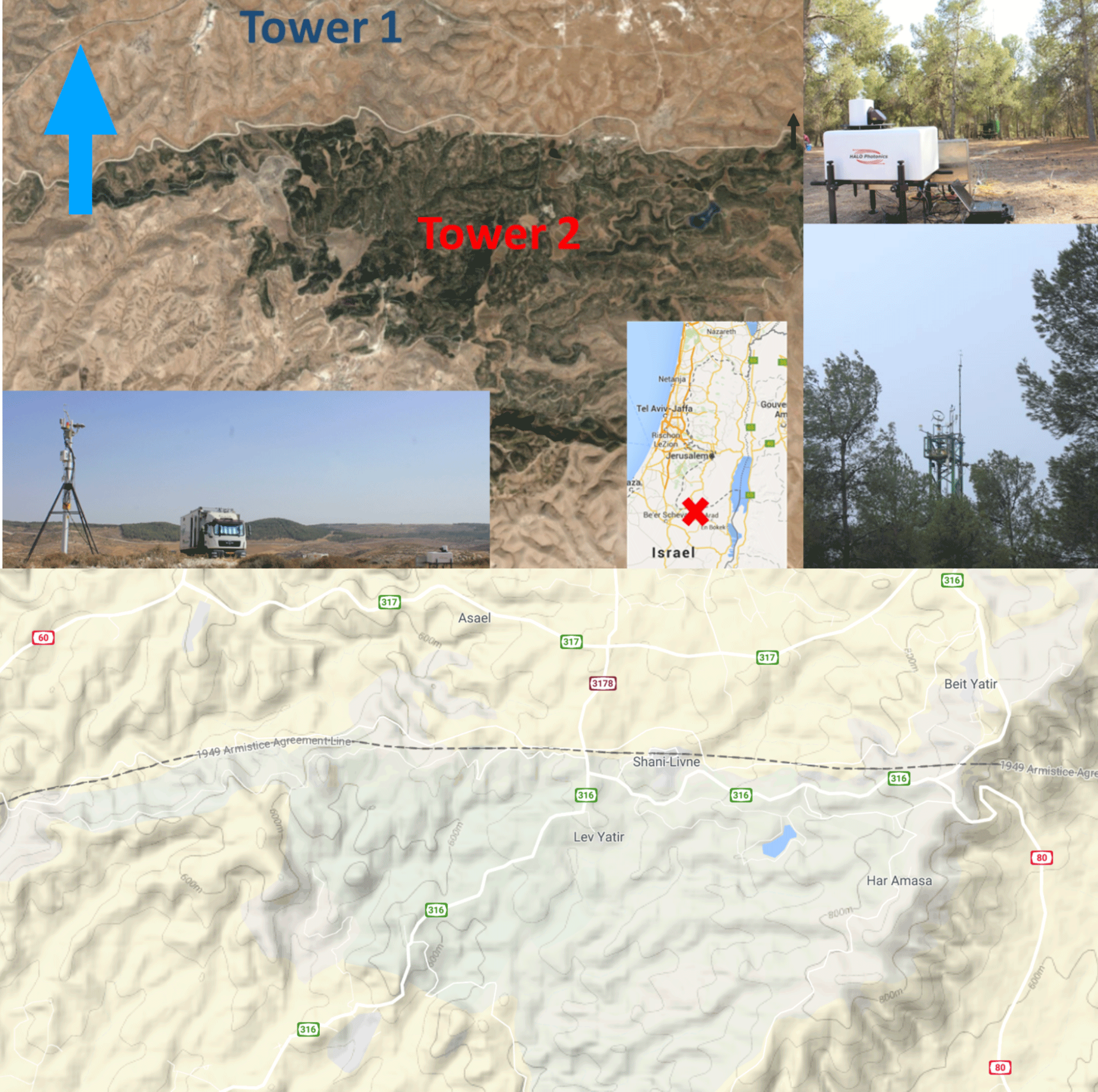
Figure 1Map of Yatir Forest in Israel and locations of the measurement stations. Insets: snapshots of measurement setups. Bottom panel: topography map of Yatir Forest from Google maps. The blue arrow indicates north.
The measurements were conducted in Yatir Forest and the surrounding shrubland in Israel between 18 and 30 August 2015 as part of the “Climate feedbacks and benefits of semi-arid forests” (CliFF) campaign, a joint collaboration between Karlsruhe Institute of Technology (KIT), Germany, and the Weizmann Institute, Israel. Figure 1 gives an idea of the locations of the EC towers. Tower 1 (lat 31.375728, long 35.024262) was located in the semiarid shrubland 620 m above sea level and tower 2 (lat 31.345315, long 35.052224) was located inside the forest 660 m above sea level. The linear distance between the two locations was measured to be 4.3 km, and as can be observed from Fig. 1, there is a distinct surface heterogeneity between the two sites. The climate of the area is in between Mediterranean and semiarid, with a mean annual precipitation of about 285 mm (Eder et al., 2015). Note that the measurement sites reported in this work are different from those in Eder et al. (2015). The trees in the forest were mostly Aleppo pine (Pinus halepensis), with an average height of 10 m with negligible height variation. The surrounding land was sparsely populated by small shrubs, and in the dry season, when the measurements were conducted, was mostly free of vegetation. Thus, it is referred to as “desert” for easy distinction (Eder et al., 2015). The measurement height for the forest was 19 m above ground (9 m above the canopy height). Note that with this height selection, the measurements were conducted above the roughness sub-layer, which ends at approximately 2 times the canopy height (Harman and Finnigan, 2007). A mast was used over the desert and the measurement height was 9 m until 23 August, after which it was changed to 15 m for the remaining period. In this zone of the atmospheric surface layer, the longitudinal and crosswise velocity variances decrease logarithmically with height and the vertical velocity variance shows independence from height (Banerjee and Katul, 2013a; Marusic et al., 2013; Perry and Chong, 1982; Townsend, 1976). High-frequency turbulent data were collected at 20 Hz and 30 min averaging periods were used for both sites. After conducting quality control of the data following Eder et al. (2015), a planar fit coordinate rotation is applied to the velocity components since the data are collected on a sloped ground. The coordinate rotation following Wilczak et al. (2001) ensures that the cross stream velocity component v is zero and corrects the tilting of the anemometer with respect to the local streamlines. Moreover, a different set of coordinate rotation is applied for the desert data after 23 August.
In addition, two Doppler lidars were used at the two locations which measured vertical velocities (Brugger et al., 2018; Kröniger et al., 2018). The Doppler lidars used were StreamLine systems from HaloPhotonics. They were operated in a vertical stare mode most of the time (interrupted every half hour for less than 90 s). Technical specifications and instrument settings of the Doppler lidars are given in Table 1. The Doppler lidar at tower 1 was not working from 19 August 2015, 15:00 UTC, until 21 August 2015, 10:30 UTC and very briefly on the 23 August 2015 around 10:00 UTC due to power cuts.
Table 1Instrument specification and settings of the Doppler lidars. From top to bottom: serial number of the forest and desert lidar, pulse length of the laser pulse at full width at half maximum, range gate length, pulse repetition frequency, number of averaged pulses for a backscatter coefficient profile, and the wavelength of the emitted laser pulse (short wavelength infrared).
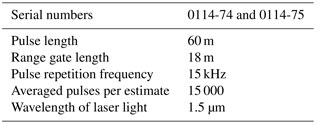
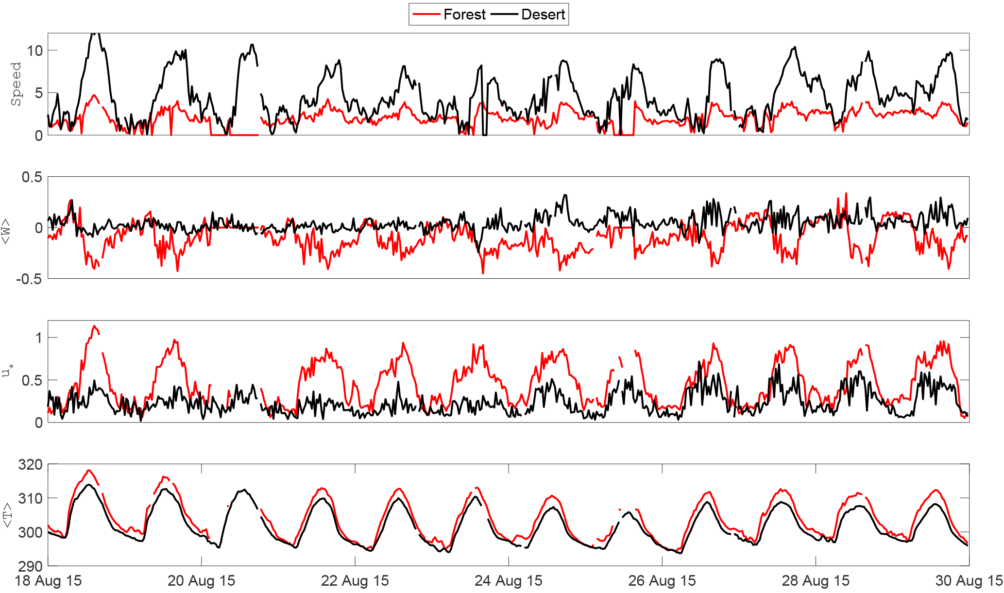
Figure 2Time series of half-hourly averages of mean speed (ms−1), mean vertical velocity (ms−1), friction velocity (ms−1) and mean potential temperature (K) for the measurement period. The black line indicates desert, and the red line indicates forest.
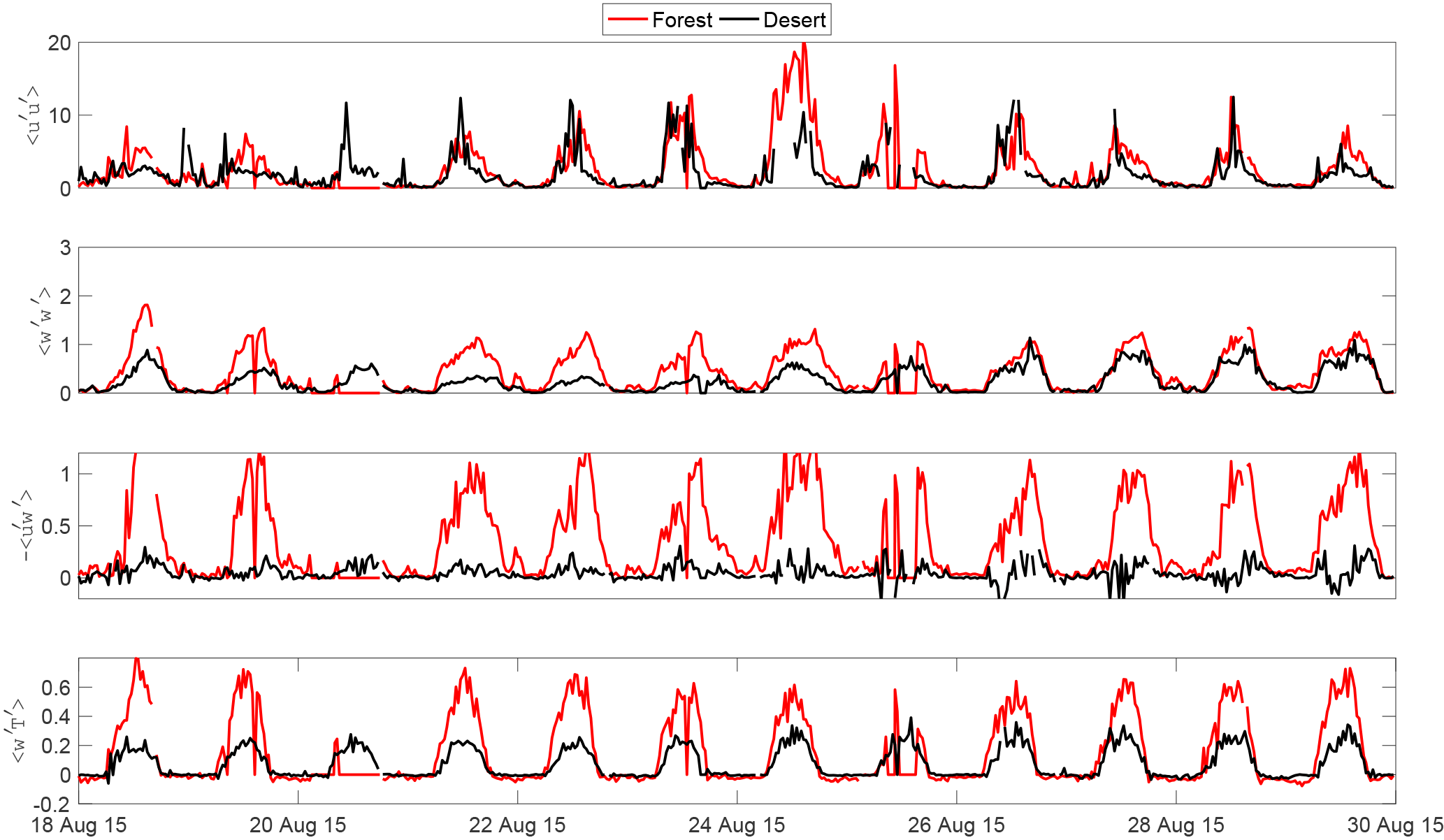
Figure 3Time series of longitudinal velocity variance (m2 s−2), vertical velocity variance (m2 s−2), momentum flux (m2 s−2) and sensible heat flux (K ms−1) for the measurement period. The black line indicates desert, and the red line indicates forest.
3.1 Time series of turbulence statistics
Time series of mean speed (ms−1), mean vertical velocity (W, ms−1) (after applying coordinate rotation), friction velocity (u*, ms−1) and mean near-surface air (potential) temperature (T, K) for the measurement period are shown in Fig. 2. Figure 3 shows time series of longitudinal velocity variance (, m2 s−2), vertical velocity variance (, m2 s−2), momentum flux (, m2 s−2) and sensible heat flux (, K ms−1). The black line indicates desert, and the red line indicates forest. As noted, the desert is associated with a higher wind speed because of a lower amount of friction on the desert surface. The higher vertical velocity over the desert indicates the presence of stronger updrafts, which would be explained by higher buoyancy-driven turbulence. The friction velocity (u*) over the forest is much higher compared to the desert, especially in the daytime, which is expected because of higher surface roughness over the forest. u*, above both the forest and the desert, shows a strong diurnal cycle. However, there seems to be a prominent increase in u* over the desert after 23 August. This can be attributed to the raising of the tower height. Moreover, the gentle topography around the desert could result in the strong vertical updrafts above the desert. Interestingly, the near-surface air temperatures over both the forest and the desert show a strong diurnal cycle and their differences are about 5 K on average during daytime and almost zero at night.
The longitudinal velocity variance over the forest and the desert show similar variations over time. The vertical velocity variance over the forest is higher than its desert counterpart; however, after 23 August, the levels of over the desert increase as well and become similar to the forest. This is due to changing the tower height. As the vertical profiles of are different between the desert and the forest (due to roughness length differences), the observed differences between are a function of observation height. At 15 m above the desert and 19 m above the forest floor, high enough to be in the “constant flux layer”, the vertical profiles of TKE () converge. However, when observed at a lower elevation and below the constant flux layer, the data show clear differences in .
The vertical momentum flux over the forest is much higher compared to the desert, which is also expected because of the higher surface roughness of the forest, making it a much more efficient momentum sink compared to the desert. Note that the shear transport of momentum flux is still much more effective over the forest compared to the desert because of roughness effects even though the mean quantities can be higher over the desert. The sensible heat flux over the forest is also higher, as discussed before, due to the canopy convector effect.
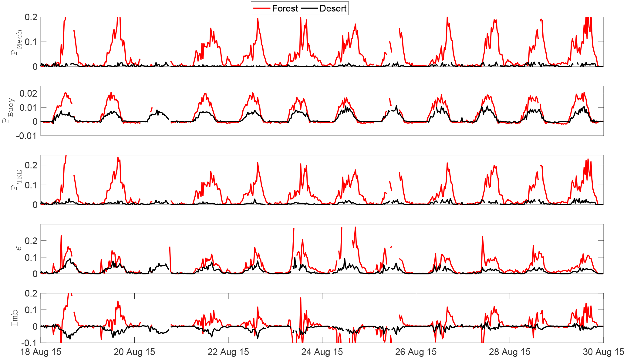
Figure 4Time series of mechanical production of TKE (m2 s−3), buoyant production of TKE (m2 s−3), full TKE production (m2 s−3), dissipation of TKE (m2 s−3) and imbalance of TKE (m2 s−3). The black line indicates desert, and the red line indicates forest.
3.2 Nature of TKE budget
Figure 4 shows the time series of the components of the TKE budget as discussed in Sect. 2.1. The first row shows mechanical production of TKE (PMech, m2 s−3); the second row shows buoyant production of TKE (PBuoy, m2 s−3); the third row shows full TKE production (PTKE, m2 s−3), which is the sum of mechanical and buoyant TKE production. The fourth row shows dissipation of TKE (ϵ, m2 s−3) and the fifth row shows an imbalance of TKE (Imb, m2 s−3). The black line indicates desert, and the red line indicates forest. As noted in Fig. 4, the production of turbulence is mostly by mechanical or shear forcing because of the roughness of the forest, whereas mechanical production of TKE over the desert is very small and does not have a strong diurnal cycle like the forest, although it increases slightly after 23 August. On the other hand, TKE production over the desert is mostly carried by buoyancy. Buoyant TKE production is slightly larger over the forest. The buoyant TKE production over the desert is also higher after 23 August. Given the moderate temperature difference between the desert and the forest, the difference in their corresponding buoyant TKE production is interesting. It also indicates that mechanical forcing and not buoyancy makes a difference (mechanical production is higher by approximately 1 order of magnitude than buoyant production) in the turbulence generation over the desert and the forest. The diurnal cycle of the TKE dissipation ϵ is interesting as well. The dissipation of TKE seems to be higher above the forest as well compared to the desert.
A smaller TKE dissipation is recorded when the measurement location is further from the ground and above the roughness sub-layer. One strong argument for observed changes after 23 August being tower-height effects rather than a change in any large-scale forcing is that changes in the desert are observed only after the 23 August, while the forest observations maintain rather consistent dynamics.
The diurnal cycles of the TKE imbalance computed by Eq. (3) are also very interesting. The imbalance over the forest is often positive over the daytime, while over the desert it is often negative, highlighting the difference in turbulent transport and advection over the two different regimes. Also note that the positive imbalance for the forest and negative imbalance for the desert almost have a phase (anti-)synchronization, indicting that the turbulence above the forest and the desert are responsive to one another and that they are part of a coupled system, indicating again the role of the secondary circulations.
3.3 Transport of TKE over the desert and the forest
Figure 5 is used to better understand the nature of turbulent transport between the desert and the forest. Panel (a) depicts the TKE imbalance over the desert vs. the net production of TKE over the forest. As observed, there is a significant correlation (0.5) between them, indicating that the advection and transport of TKE by flux divergence and pressure fluctuations reach downstream by means of the secondary circulations and produce TKE over the forest. On the other hand, the reverse is not true, as observed in panel (b) of Fig. 5. There is little correlation between the imbalance of TKE over the forest and the production of TKE over the desert (0.14). As observed in panel (c), the production over the desert is also well correlated with the production over the forest (0.3) as both the desert and the forest are subject to the same forcing. However, the TKE production over the desert is not that well correlated with the TKE imbalance over the desert as seen in panel (d). Thus, while there should be some cross correlation in panel (a) because of desert production, that is not the only effect. The nonlocal large-scale motions contribute to the transport over the desert (without significantly altering TKE production over the desert) which in turn cause TKE production above the forest because of the higher mechanical forcing.
Thus, it can be stated that at least in the canopy sub-layer and in the atmospheric surface layer, the effects of secondary circulations are transported from over the desert towards the forest following the background wind direction, and it is not the other way around. It is worth noting here that the term “secondary circulation” has been used somewhat loosely here and contain the effects of horizontal transport as well, since partitioning the imbalance term is not possible within the scope of this campaign. In the case of transport from the forest towards the desert, it is more likely that horizontal advection is the main mechanism. The nature of the full extent of the secondary circulation are a part of a much larger flow pattern and are not fully captured by the eddy covariance towers, which only capture the fine-scale turbulence. To reveal the full nature of the secondary circulations, one can look at lidar observations as shown in Appendix B (Brugger et al., 2018) as well as large eddy simulations (Kröniger et al., 2018).
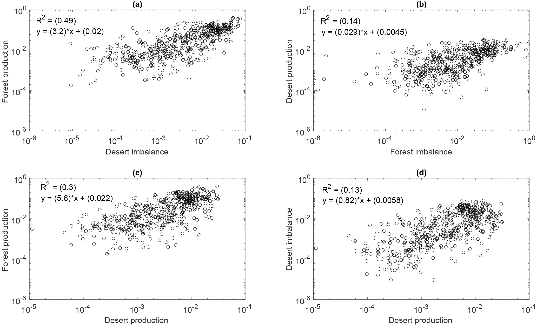
Figure 5(a) TKE imbalance for the desert vs. TKE production for the forest. (b) TKE imbalance for the forest vs. TKE production for the desert. (c) TKE production for the desert vs. TKE production for the forest. (d) TKE production for the desert vs. TKE imbalance for the desert. Significance: 0.05 level.
3.4 Effect of nonlocal motions
Figure 6 shows the time series of the triple moments , and in the first three rows. The vertical velocity skewness term (second row) is of importance as it appears in the transport term of the TKE budget (Eq. 2) and is a measure of non-Gaussian turbulence, which indicates the presence of nonlocal coherent motions such as sweeps and ejections. Note that the vertical velocity skewness is often negative above the canopy, which is consistent with the generic feature of canopy turbulence (Chamecki, 2013; Dias-Junior et al., 2015; Kaimal and Finnigan, 1994). The daytime vertical velocity skewness over the desert is often positive, indicating again the presence of nonlocal coherent structures active over the desert. The measure of skewness increases over the desert after 23 August, which is also due to the height change. The other two terms and are also associated with turbulent transport of momentum and heat as evident from their respective budget equations (Banerjee et al., 2017b; Cava et al., 2006; Katul et al., 2013; Raupach et al., 1986; Zhuang and Amiro, 1994).
and
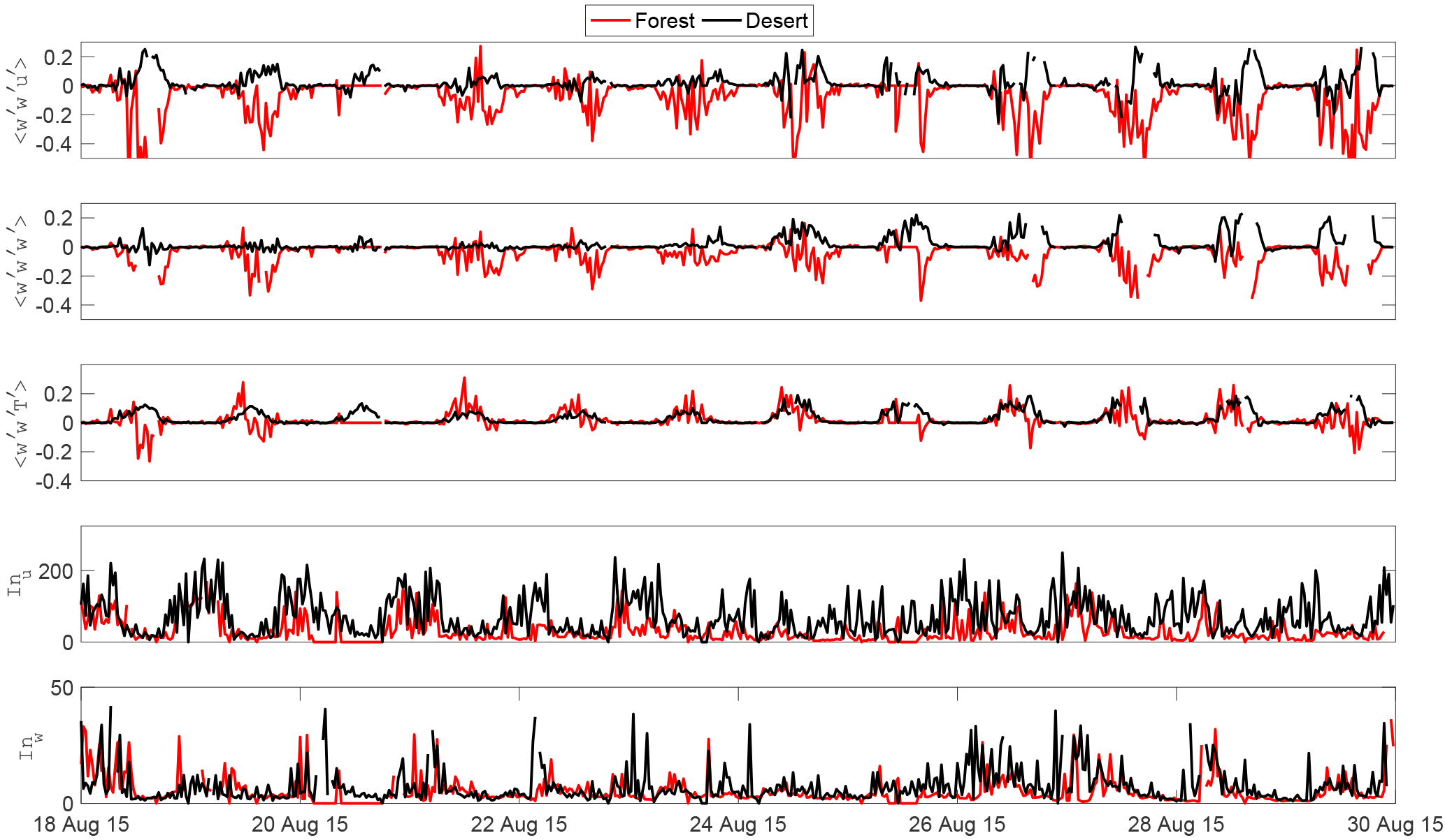
Figure 6Top three panels: time series of triple moments , (m3 s−3) and (K m2 s−2). Bottom two panels show the integral timescales of horizontal (Inu) and vertical velocities (Inw) in seconds.
Moreover, the triple moments have been shown to be directly correlated with the relative contributions of nonlocal events such as sweeps and ejections (Banerjee et al., 2017b; Cava et al., 2006; Katul et al., 2013; Nakagawa and Nezu, 1977; Raupach et al., 1986). Note that momentum transport term is also opposite in sign for the desert and the forest, and it shows a strong diurnal cycle. After 23 August, an increase in momentum transport is noted for the desert. However, the diurnal cycle of the heat transport term is not as strong as its momentum counterpart, but it is often found to be larger over the desert compared to the forest, consistent with the findings from the TKE budget that show heat is transported from over the desert towards the forest. It is, however, important to note that the structures are representative of the fine-scale turbulence and not directly representative of the large-scale circulation structures spanning the whole boundary layer. The fourth and fifth rows of Fig. 6 show the time series of the integral timescale of horizontal (Inu) and vertical (Inw) velocity components in seconds. Inu and Inw for every half hour time period are computed by integrating the normalized autocorrelation function of u and w until the first zero crossing (Kaimal and Finnigan, 1994). They can be interpreted as the characteristic timescale of the most energetic eddies in each direction. As noted in Fig. 6, timescales in the horizontal directions are larger compared to the vertical direction. More interesting is the observation that the integral timescales for the eddies above the desert are larger than those above the forest, which also increase after 23 August. This is another indicator of buoyant production of turbulence, which generates larger eddies than shear production.
We studied the nature of turbulent transport over a well-defined surface heterogeneity, comprising a desert and forest in the Yatir semiarid area in Israel. Eddy covariance and Doppler lidar measurements were conducted for 12 days between 18 and 31 August 2015 over two locations in the forest and the shrubland (referred to as “desert” because of the almost complete lack of vegetation during the observation period). Earlier campaigns in this area focused on energy balance closure and hypothesized that there are secondary circulations because of surface heterogeneity. The present work was aimed to study the nature of turbulent transport over the forest and the desert in more detail to address the following questions:
-
How does Yatir Forest affect the boundary layer dynamics such as eddy size distribution, boundary layer height and diurnal variations in turbulent statistics and fluxes compared to the surrounding desert?
-
Can the existence of secondary circulation be confirmed?
-
Is there any horizontal energy transport between the forest and the desert and how does it vary with time?
To answer the abovementioned questions, we computed half hour average turbulent statistics for both the desert and the forest and looked at their diurnal variations. We also computed individual components of the turbulent kinetic energy (TKE) budget and argued that the turbulent transport of energy should be contained in the imbalance of the TKE budget, which consists of the effects of advection, transport by turbulent flux divergence and pressure velocity interactions, since we could not compute those terms explicitly. Moreover, we also computed triple moments, which are associated with nonlocal motions and coherent structures, and integral timescales, which are associated with the most energetic eddies. The findings to the questions are listed below.
-
The forest is found to be associated with a higher level of turbulent intensity because of higher roughness although the desert had higher mean speeds and vertical updrafts, possibly due to the presence of secondary circulations. Gentle topography around the desert might contribute to the updrafts over the desert as well. The higher roughness of the desert is also responsible for higher wind speeds above the desert. There is little air temperature difference between the desert and the forest, although the mean velocities and temperature have strong diurnal cycles. Momentum and heat flux are also found to be stronger above the forest. The presence of the secondary circulation enhances the turbulent fluxes as well as the turbulent intensity above the desert.
-
The role of secondary circulations can be better understood once the components of the TKE budget are studied. Over the forest, the production of turbulence is mechanical, while over the desert, TKE production is mostly carried by buoyancy. The forest is more efficient in dissipating TKE as well. The imbalance of TKE is taken as the indicator of TKE transport and is found to vary diurnally almost anti-synchronously over the desert and the forest, confirming the role of a secondary circulation. The TKE budget is closed better over the forest compared to the desert. Turbulent triple moments, which are indicators of nonlocal motions and coherent structures, also show strong variability over the desert and are opposite in signs also confirming the role of secondary circulations. The integral timescales are found to be greater over the desert compared to the forest. This suggests that the secondary circulations that transport energy are more active over the desert – however, they cannot produce much turbulence over the desert since they only rely on buoyancy-driven turbulence as mechanical forcing is missing over the desert. This is also highlighted by the fact that mean velocities are higher above the desert while turbulent fluctuations are higher above the forest.
-
To elucidate the role of horizontal transport between the desert and the forest, we studied the correlation between the TKE imbalance over the desert and the TKE production over the forest. The moderately high correlation suggests that the secondary circulation is transported from over the desert towards the forest, enhancing TKE production over the forest, at least in the canopy sub-layer and the atmospheric surface layer. The low correlation between the TKE imbalance over the forest and TKE production over the desert confirms the directionality of this horizontal exchange, which is from the desert towards the forest and not the other way around.
To summarize, we have examined the existence and role of secondary circulations that exists because of large-scale surface heterogeneities and possible due to some topography effects between the desert and the forest by looking at proxy quantities computed from turbulence measurements. Although the campaign was conducted at a particular site, the conclusions drawn are fairly general and can be extended to other scenarios involving surface heterogeneities, such as urban landscapes and agricultural fields. Future work will attempt to highlight a more spatially detailed picture of the turbulent structure under the interesting scenario of secondary circulations and horizontal energy transport.
We suggest contacting the principal investigator Matthias Mauder (matthias.mauder@kit.edu) if readers are interested in obtaining the data used in the paper.
Thus, to be consistent, with Eq. (2), all the terms in Eq. (A1) that cannot be evaluated using one-point measurements can be clubbed in the imbalance term, which can be described by
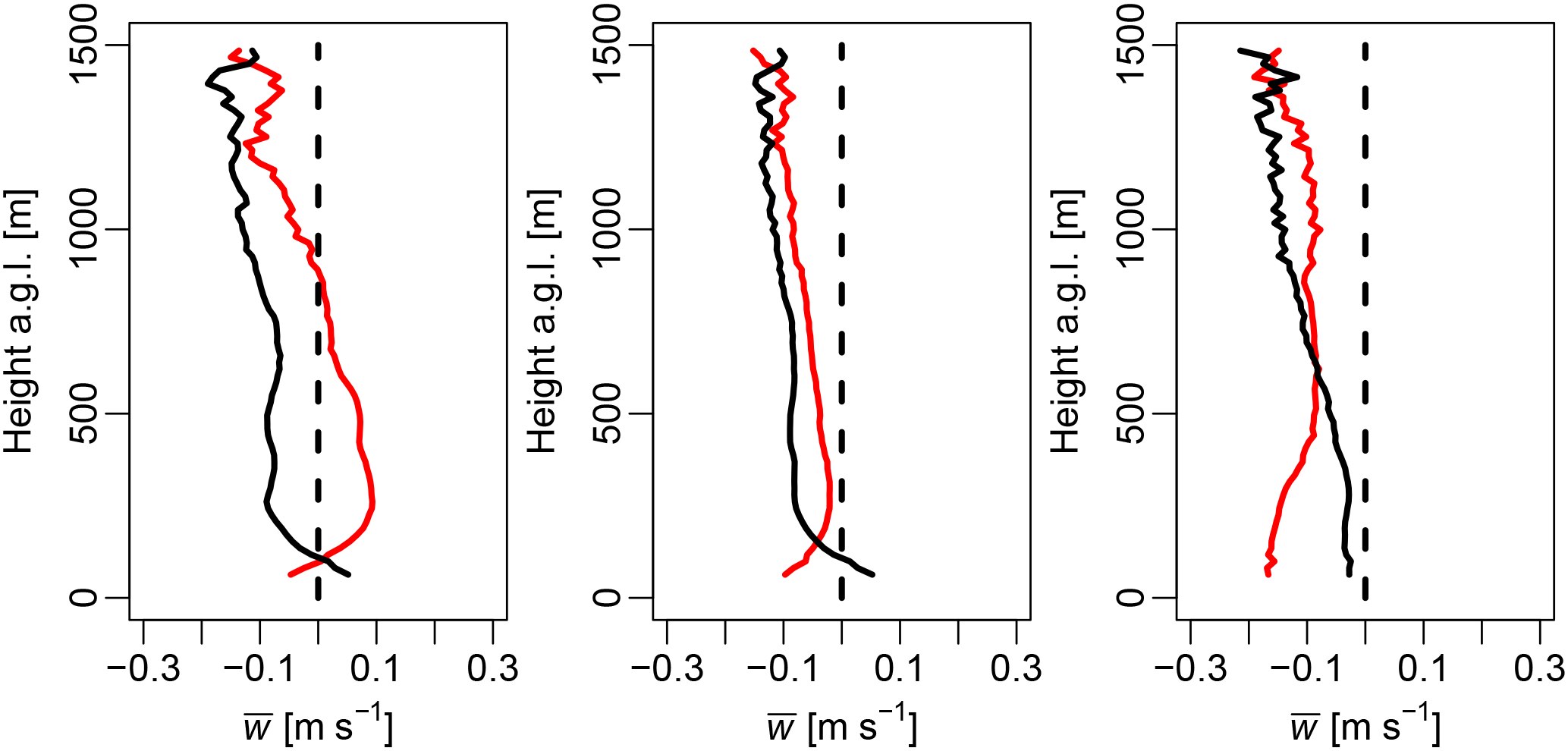
Figure A1Vertical mean velocity profile averaged from 18 to 29 August (only times with both instruments simultaneously online and the nearest three range gates are discarded). Left to right: 4 h window centered on noon, daytime (sunrise to sundown) and nighttime (sundown to sunrise). The forest is shown as a solid red line, the desert as solid black line and a vertical line at as a black dashed line. Note that near the surface, the desert always has larger w, but only during the noontime with the updrafts of the forest is there a change in sign.
Thus, if no assumptions or idealizations are invoked, the imbalance of the commonly used operational TKE budget (Eq. 2) consists of TKE tendency, advection, shear production, TKE flux divergence and pressure velocity interactions. Using an array of sonics in each direction will enable determination of all these terms. However, as evident from the myriad of terms contributing to the imbalance, it is difficult to determine what degree of assumptions of homogeneity in which direction are sufficient so that certain terms can be ignored. Thus, unless all terms in Eq. (A2) can be determined, it is easier to stick to the most idealized form of Eq. (2) and treat all other terms as imbalances. Future work will try to determine the partitioning of advection, flux divergence and the other shear production terms contributing to TKE budget imbalances in the presence of heterogeneities.
Figure A1 shows mean vertical velocity W above the forest and the desert averaged over all observations using the Doppler lidars. Secondary circulation cannot be thought of as a single large rotational system spanning the desert and the forest; rather, it is a much more complex and three-dimensional structure. Close to the surface layer and the canopy sub-layer, the transport of energy is indeed from the desert to the forest (Fig. 5). Further, we observe that the desert has more updrafts and the forest has more downdrafts close to the surface. However, as we go up above roughly 100 m, this behavior flips. Lastly, Kröniger et al. (2018) found in his simulations that large rotational systems developed at specific locations connected to surface features. Therefore, we conclude that the bulk transport in the convective mixed layer by a secondary circulation is from the forest to the desert, but it is advected with the mean wind and heavily influenced by surface features on a smaller scale than the forest itself.
TB did the data analysis and wrote the paper. PB collected the data, FDR, and KK helped in the interpretation. MM, DY and EY oversaw the whole project and was involved in the entire workflow, starting from data collection to data analysis and interpretation.
The authors declare that they have no conflict of interest.
This research was supported by the German Research Foundation (DFG) as part
of the project “Climate feedbacks and benefits of semi-arid forests”
(CliFF) and the project “Capturing all relevant scales of
biosphere–atmosphere exchange – the enigmatic energy balance closure
problem”, which is funded by the Helmholtz-Association through the
President's Initiative and Networking Fund and by KIT.
The article processing
charges for this open-access
publication were covered by a
Research
Centre of the Helmholtz Association.
Edited by: Thomas Karl
Reviewed by: Gil Bohrer
and one anonymous referee
Banerjee, T. and Katul, G.: Logarithmic scaling in the longitudinal velocity variance explained by a spectral budget, Phys. Fluids (1994–present), 25, 125106, https://doi.org/10.1063/1.4837876, 2013a. a
Banerjee, T., Katul, G., Fontan, S., Poggi, D., and Kumar, M.: Mean flow near edges and within cavities situated inside dense canopies, Bound.-Lay. Meteorol., 149, 19–41, 2013. a, b
Banerjee, T., Katul, G., Salesky, S., and Chamecki, M.: Revisiting the formulations for the longitudinal velocity variance in the unstable atmospheric surface layer, Q. J. Roy. Meteorol. Soc., 141, 1699–1711, 2015. a
Banerjee, T., Li, D., Juang, J.-Y., and Katul, G.: A spectral budget model for the longitudinal turbulent velocity in the stable atmospheric surface layer, J. Atmos. Sci., 73, 145–166, 2016. a, b
Banerjee, T., De Roo, F., and Mauder, M.: Explaining the convector effect in canopy turbulence by means of large-eddy simulation, Hydrol. Earth Syst. Sci., 21, 2987–3000, https://doi.org/10.5194/hess-21-2987-2017, 2017a. a
Banerjee, T., De Roo, F., and Mauder, M.: Connecting the Failure of K Theory inside and above Vegetation Canopies and Ejection–Sweep Cycles by a Large-Eddy Simulation, J. Appl. Meteorol. Climatol., 56, 3119–3131, 2017b. a, b
Belcher, S. E., Jerram, N., and Hunt, J. C. R.: Adjustment of a Turbulent Boundary Layer to a Canopy of Roughness Elements, J. Fluid Mech., 488, 369–398, 2003. a
Brugger, P., Banerjee, T., De Roo, F., Kröniger, K., Qubaja, R., Rohatyn, S., Rotenberg, E., Tatarinov, F., Yakir, D., Yang, F., and Mauder, M.: Effect of Surface Heterogeneity on the Boundary-Layer Height: A Case Study at a Semi-Arid Forest, Bound.-Lay. Meteorol., 1–18, 2018. a, b
Businger, J. A., Wyngaard, J. C., Izumi, Y., and Bradley, E. F.: Flux-profile relationships in the atmospheric surface layer, J. Atmos. Sci., 28, 181–189, 1971. a
Cassiani, M., Katul, G. G., and Albertson, J. D.: The Effects of Canopy Leaf Area Index on Airflow across Foest Edges: Large-Eddy Simulation and Analytical Results, Bound.-Lay. Meteorol., 126, 433–460, 2008. a
Cava, D., Katul, G., Scrimieri, A., Poggi, D., Cescatti, A., and Giostra, U.: Buoyancy and the sensible heat flux budget within dense canopies, Bound.-Lay. Meteorol., 118, 217–240, 2006. a, b
Chamecki, M.: Persistence of velocity fluctuations in non-Gaussian turbulence within and above plant canopies, Phys. Fluids (1994–present), 25, 115110, https://doi.org/10.1063/1.4832955, 2013. a
Chatziefstratiou, E. K., Velissariou, V., and Bohrer, G.: Resolving the effects of aperture and volume restriction of the flow by semi-porous barriers using large-eddy simulations, Bound.-Lay. Meteorol., 152, 329–348, 2014. a
Courault, D., Drobinski, P., Brunet, Y., Lacarrere, P., and Talbot, C.: Impact of surface heterogeneity on a buoyancy-driven convective boundary layer in light winds, Bound.-Lay. Meteorol., 124, 383–403, 2007. a
Dalpe, B. and Masson, C.: Numerical Simulation of Wind Flow near a Forest Edge, J. Wind Eng. Ind. Aerod., 97, 228–241, 2009. a
Dalu, G. and Pielke, R.: Vertical heat fluxes generated by mesoscale atmospheric flow induced by thermal inhomogeneities in the PBL, J. Atmos. Sci., 50, 919–926, 1993. a
Detto, M., Katul, G. G., Siqueira, M., Juang, J. Y., and Stoy, P.: The Structure of Turbulence near a Tall Forest Edge: The Backward-Facing Step Flow Analogy Revisited, Ecological Applications, 18, 1420–1435, 2008. a
Dias-Junior, C. Q., Marques Filho, E. P., and Sá, L. D.: A large eddy simulation model applied to analyze the turbulent flow above Amazon forest, J. Wind Eng. Ind. Aerod., 147, 143–153, 2015. a
Dixon, N., Parker, D., Taylor, C., Garcia-Carreras, L., Harris, P., Marsham, J., Polcher, J., and Woolley, A.: The effect of background wind on mesoscale circulations above variable soil moisture in the Sahel, Q. J. Roy. Meteorol. Soc., 139, 1009–1024, 2013. a
Dupont, S. and Brunet, Y.: Coherent structures in canopy edge flow: a large-eddy simulation study, J. Fluid Mech., 630, 93–128, 2009. a
Dyer, A.: A review of flux-profile relationships, Bound.-Lay. Meteorol., 7, 363–372, 1974. a
Eder, F., De Roo, F., Kohnert, K., Desjardins, R. L., Schmid, H. P., and Mauder, M.: Evaluation of two energy balance closure parametrizations, Bound.-Lay. Meteorol., 151, 195–219, 2014. a
Eder, F., De Roo, F., Rotenberg, E., Yakir, D., Schmid, H. P., and Mauder, M.: Secondary circulations at a solitary forest surrounded by semi-arid shrubland and their impact on eddy-covariance measurements, Agr. Forest Meteorol., 211, 115–127, 2015. a, b, c, d, e, f, g, h, i
Fesquet, C., Dupont, S., Drobinski, P., Dubos, T., and Barthlott, C.: Impact of Terrain Heterogeneity on Coherent Structure Properties: Numerical Approach, Bound.-Lay. Meteorol., 133, 71–92, 2009. a
Foken, T.: The energy balance closure problem: an overview, Ecol. Appl., 18, 1351–1367, 2008. a
Fuentes, J. D., Chamecki, M., Nascimento dos Santos, R. M., Von Randow, C., Stoy, P. C., Katul, G., Fitzjarrald, D., Manzi, A., Gerken, T., Trowbridge, A., Souza Freire, L., Ruiz-Plancarte, J., Furtunato Maia, J. M., Tóta, J., Dias, N., Fisch, G., Schumacher, C., Acevedo, O., Rezende Mercer, J., and Yañez-Serrano, A. M.: Linking meteorology, turbulence, and air chemistry in the Amazon rainforest, B. Am. Meteorol. Soc., 97, 2329–2342, 2016. a
Garcia-Carreras, L., Parker, D. J., Taylor, C. M., Reeves, C. E., and Murphy, J. G.: Impact of mesoscale vegetation heterogeneities on the dynamical and thermodynamic properties of the planetary boundary layer, J. Geophys. Res.-Atmos., 115, https://doi.org/10.1029/2009JD012811, 2010. a
Gavrilov, K., Accary, G., Morvan, D., Lyubimov, D., Bessonov, O., and Meradji, S.: Large Eddy Simulation of Coherent Structures over Forest Canopy, Turbulence and Interactions, 110, 143–149, 2010. a
Gavrilov, K., Accary, G., Morvan, D., Lyubimov, D., Meradji, S., and Bessonov, O.: Numerical Simulation of Coherent Structures over Plant Canopy, Flow Turbulence and Combustion, 86, 89–111, 2011. a
Harman, I. N. and Finnigan, J. J.: A simple unified theory for flow in the canopy and roughness sublayer, Bound.-Lay. Meteorol., 123, 339–363, 2007. a
Higgins, C. W., Katul, G. G., Froidevaux, M., Simeonov, V., and Parlange, M. B.: Are atmospheric surface layer flows ergodic?, Geophys. Res. Lett., 40, 3342–3346, 2013. a
Huang, J., Cassiani, M., and Albertson, J. D.: Coherent Turbulent Structures across a Vegetation Discontinuity, Bound.-Lay. Meteorol., 140, 1–22, 2011. a
Irvine, M. R., Gardiner, B. A., and Hill, M. K.: The Evolution of Turbulence across a Forest Edge, Bound.-Lay. Meteorol., 84, 467–496, 1997. a
Kaimal, J. C. and Finnigan, J. J.: Atmospheric boundary layer flows: their structure and measurement, Oxford University Press, 1994. a, b, c
Kanani-Sühring, F. and Raasch, S.: Spatial variability of scalar concentrations and fluxes downstream of a clearing-to-forest transition: a large-eddy simulation study, Bound.-Lay. Meteorol., 155, 1–27, 2015. a
Kanda, M., Inagaki, A., Letzel, M. O., Raasch, S., and Watanabe, T.: LES study of the energy imbalance problem with eddy covariance fluxes, Bound.-Lay. Meteorol., 110, 381–404, 2004. a
Kang, S.-L. and Lenschow, D. H.: Temporal evolution of low-level winds induced by two-dimensional mesoscale surface heat-flux heterogeneity, Bound.-Lay. Meteorol., 151, 501–529, 2014. a
Katul, G. G., Cava, D., Siqueira, M., and Poggi, D.: Scalar turbulence within the canopy sublayer, Coherent Flow Structures at Earth's Surface, chap. 6, 73–95, 2013. a, b
Kröniger, K., Banerjee, T., De Roo, F., and Mauder, M.: Flow adjustment inside homogeneous canopies after a leading edge–An analytical approach backed by LES, Agr. Forest Meteorol., 255, 17–30, https://doi.org/10.1016/j.agrformet.2017.09.019, 2017. a
Kröniger, K., , DeRoo, F., Brugger, P., Huq, S., Banerjee, T., Zinsser, J., Rotenberg, E., Yakir, D., Rohatyn, S., and Mauder, M.: Effect of Secondary Circulations on the Surface–Atmosphere Exchange of Energy at an Isolated Semi-arid Forest, Bound.-Lay. Meteorol., https://doi.org/10.1007/s10546-018-0370-6, 2018. a, b, c
Li, D., Salesky, S. T., and Banerjee, T.: Connections between the Ozmidov scale and mean velocity profile in stably stratified atmospheric surface layers, J. Fluid Mech., 797, https://doi.org/10.1017/jfm.2016.311, 2016. a, b
Li, Z. J., Lin, J. D., and Miller, D. R.: Air-Flow over and through a Forest Edge – a Steady-State Numerical-Simulation, Bound.-Lay. Meteorol., 51, 179–197, 1990. a
Mahfouf, J.-F., Richard, E., and Mascart, P.: The influence of soil and vegetation on the development of mesoscale circulations, J. Appl. Meteorol. Climatol., 26, 1483–1495, 1987. a
Markfort, C., Porté-Agel, F., and Stefan, H.: Canopy-wake dynamics and wind sheltering effects on Earth surface fluxes, Environ. Fluid Mech., 14, 663–697, 2014. a
Marusic, I., Monty, J. P., Hultmark, M., and Smits, A. J.: On the logarithmic region in wall turbulence, J. Fluid Mech., 716, https://doi.org/10.1017/jfm.2012.511, 2013. a
Mauder, M., Jegede, O., Okogbue, E., Wimmer, F., and Foken, T.: Surface energy balance measurements at a tropical site in West Africa during the transition from dry to wet season, Theor. Appl. Climatol., 89, 171–183, 2007. a
Monin, A. and Obukhov, A.: Basic laws of turbulent mixing in the surface layer of the atmosphere, Contrib. Geophys. Inst. Acad. Sci. USSR, 151, 163–187, 1954. a
Nadeau, D. F., Pardyjak, E. R., Higgins, C. W., Fernando, H. J. S., and Parlange, M. B.: A simple model for the afternoon and early evening decay of convective turbulence over different land surfaces, Bound.-Lay. Meteorol., 141, 301–324, https://doi.org/10.1007/s10546-011-9645-x, 2011. a, b
Nakagawa, H. and Nezu, I.: Prediction of the contributions to the Reynolds stress from bursting events in open-channel flows, J. Fluid Mech., 80, 99–128, 1977. a
Peltola, H.: Model Computations on Wind Flow and Turning Moment for Scots Pine s along the Margins of Clear-Cut Areas, Forest Ecol. Manage., 83, 203–215, 1996. a
Perry, A. and Chong, M.: On the mechanism of wall turbulence, J. Fluid Mech., 119, 173–217, 1982. a
Queck, R., Bernhofer, C., Bienert, A., and Schlegel, F.: The TurbEFA Field Experiment – Measuring the Influence of a Forest Clearing on the Turbulent Wind Field, Bound.-Lay. Meteorol., 160, 397–423, 2016. a
Raupach, M. and Finnigan, J.: Scale issues in boundary-layer meteorology: Surface energy balances in heterogeneous terrain, Hydrol. Process., 9, 589–612, 1995. a, b
Raupach, M., Coppin, P., and Legg, B.: Experiments on scalar dispersion within a model plant canopy part I: The turbulence structure, Bound.-Lay. Meteorol., 35, 21–52, 1986. a, b
Rominger, J. T. and Nepf, H. M.: Flow Adjustment and Interior Flow Associated with a Rectangular Porous Obstruction, J. Fluid Mech., 680, 636–659, 2011. a
Rotenberg, E. and Yakir, D.: Distinct patterns of changes in surface energy budget associated with forestation in the semiarid region, Glob. Change Biol., 17, 1536–1548, 2011. a
Salesky, S. T., Katul, G. G., and Chamecki, M.: Buoyancy effects on the integral lengthscales and mean velocity profile in atmospheric surface layer flows, Phys. Fluids (1994–present), 25, 105101, https://doi.org/10.1063/1.4823747, 2013. a
Schlegel, F., Stiller, J., Bienert, A., Maas, H. G., Queck, R., and Bernhofer, C.: Large-Eddy Simulation of Inhomogeneous Canopy Flows Using High Resolution Terrestrial Laser Scanning Data, Bound.-Lay. Meteorol., 142, 223–243, 2012. a
Stoy, P. C., Mauder, M., Foken, T., Marcolla, B., Boegh, E., Ibrom, A., Arain, M. A., Arneth, A., Aurela, M., Bernhofer, C., et al.: A data-driven analysis of energy balance closure across FLUXNET research sites: The role of landscape scale heterogeneity, Agr. Forest Meteorol., 171, 137–152, 2013. a
Stull, R. B.: An introduction to boundary layer meteorology, vol. 13, Springer Science & Business Media, 2012. a, b, c
Sühring, M. and Raasch, S.: Heterogeneity-induced heat-flux patterns in the convective boundary layer: can they be detected from observations and is there a blending height? – a large-eddy simulation study for the LITFASS-2003 experiment, Bound.-Lay. Meteorol., 148, 309–331, 2013. a
Townsend, A. A.: The structure of turbulent shear flow, Cambridge University Press, 1976. a
van Heerwaarden, C. C. and Guerau de Arellano, J. V.: Relative humidity as an indicator for cloud formation over heterogeneous land surfaces, J. Atmos. Sci., 65, 3263–3277, 2008. a
Van Heerwaarden, C. C., Mellado, J. P., and De Lozar, A.: Scaling laws for the heterogeneously heated free convective boundary layer, J. Atmos. Sci., 71, 3975–4000, 2014. a
Wilczak, J. M., Oncley, S. P., and Stage, S. A.: Sonic anemometer tilt correction algorithms, Bound.-Lay. Meteorol., 99, 127–150, 2001. a
Yang, B., Raupach, M. R., Shaw, R. H., Tha, K., Paw, U., and Morse, A. P.: Large-Eddy Simulation of Turbulent Flow across a Forest Edge. Part I: Flow Statistics, Bound.-Lay. Meteorol., 120, 377–412, 2006. a
Yue, P., Zhang, Q., Wang, R., Li, Y., and Wang, S.: Turbulence intensity and turbulent kinetic energy parameters over a heterogeneous terrain of Loess Plateau, Adv. Atmos. Sci., 32, 1291–1302, 2015. a, b
Zhuang, Y. and Amiro, B.: Pressure fluctuations during coherent motions and their effects on the budgets of turbulent kinetic energy and momentum flux within a forest canopy, J. Appl. Meteorol., 33, 704–711, 1994. a