Analysis of Antarctic ozone trends from 1979 to 2023

Antarctic column ozone has shown signs of a sustained recovery since 2000, but levels were distinctly low during 2020–2022, potentially affecting estimates of ozone recovery and long-term trends. To assess the impact of recent low ozone on long-term variability, we analyse total column ozone (TCO) data from the World Ozone and Ultraviolet Radiation Centre, multi-sensor reanalysis, and Total Ozone Mapping Spectrometer/Ozone Monitoring Instrument. Ozone fields from the TOMCAT 3-D chemical transport model are also used to gain better insight into the changes. Multiple linear regression (MLR) is applied to estimate ozone trends over Antarctica from 1979 to 2023, incorporating proxies representing key chemical and dynamical processes such as the El Niño-Southern Oscillation and the Brewer–Dobson circulation (BDC).

Our analysis confirms that TCO declined across all datasets before 2000. The annual mean decreased at a rate of 2 Dobson units per year (DU yr⁻¹), while more pronounced decreases of approximately 6 DU yr⁻¹ occurred in September and October. For the 2001–2019 period, TCO showed signs of recovery in the annual mean (0.5 DU yr⁻¹) and September (1.5 DU yr⁻¹), while the annual trend shifted to −0.4 DU yr⁻¹ and September trend was near zero over the extended 2001–2023 period. The MLR effectively captures long-term ozone changes as well as unusual dynamical events such as the sudden stratospheric warmings in 2002 and 2019. Annual mean and springtime (September/October) TCO exhibited a positive correlation with the estimated BDC contribution throughout the 2001–2023 period. As dynamical proxies show the largest influence, we use TOMCAT simulations to illustrate the impact of the BDC on the Antarctic ozone. Two sensitivity simulations further demonstrate that the strengthening (weakening) of the circulation leads to high (low) ozone values in spring. Cold temperatures and abnormal BDC in 2021–2022 resulted in low ozone levels. These findings suggest that now ozone-depleting substances have been effectively controlled, dynamical processes are playing an increasingly important role in controlling the ozone recovery patterns in Antarctica.

1 Introduction

The discovery of the Antarctic ozone hole in 1985 sparked decades of intensive research on the causes of stratospheric ozone depletion and its broader climate implications (Farman et al., 1985; Solomon et al., 1986). Early scientific studies correctly established the link between the decline in Antarctic ozone and anthropogenic emissions of halogenated ozone-depleting substances (ODSs), such as trichlorofluoromethane (CFC-11) and dichlorodifluoromethane (CFC-12) (WMO, 2014, 2018, 2022). These and similar compounds historically contributed a large portion of the stratospheric chlorine loading. In response to this environmental threat, the 1987 Montreal Protocol and its subsequent amendments were successfully implemented which has led to ongoing reductions in the stratospheric chlorine and bromine loadings (WMO, 2022). Beyond their role in ozone depletion, these halogenated substances are also potent greenhouse gases with high global warming potentials, meaning their phase-out has provided substantial co-benefits for climate change mitigation (e.g. Ramanathan et al., 1985; Velders et al., 2007).

These regulatory measures led to stabilisation in global ozone trends and initiated a gradual recovery toward pre-1980 conditions (e.g. Dhomse et al., 2018; WMO, 2022). Significant signs of recovery have been confirmed in the upper stratosphere, where ozone increases are attributed to both declining halogens and stratospheric cooling resulting from increased greenhouse gas abundances (Steinbrecht et al., 2017; Chipperfield et al., 2017; Godin-Beekmann et al., 2022). However, the evolution of the lower stratosphere remains a subject of ongoing debate and high uncertainty (e.g. Chipperfield et al., 2018). Several observation-based studies suggest a continued decline in lower-stratospheric ozone since 1998, which has been linked to changes in stratospheric dynamics and increased tropical upwelling (Ball et al., 2018; Wargan et al., 2018). In the Antarctic region specifically, while a sustained recovery has been observed in September since 2000 (Solomon et al., 2016), the period between 2020 and 2023 was characterized by exceptionally large and long-lasting ozone holes (Kessenich et al., 2023; Wang et al., 2025). The accurate quantification of how these recent perturbations affect long-term recovery trends remains unclear.

Antarctic ozone variability depends not only on declining halogens but also on a complex interplay of chemical and dynamical processes that vary across multiple timescales. External climate forcings, such as 11-year solar variability and sporadic volcanic eruptions, exert a significant influence on polar ozone levels (e.g. Dhomse et al., 2016, 2022). Increased ultraviolet radiation during solar maxima enhances ozone production in the upper stratosphere (Gray et al., 2010). Major volcanic events, such as Mount Pinatubo in 1991, have caused significant mid-latitude ozone depletion through heterogeneous chemical processing on sulphate aerosols (Aquila et al., 2013; Dhomse et al., 2015). More recently, the 2022 eruption of the Hunga volcano and major wildfires, such as the 2019–2020 Australian fires, have been identified as significant perturbations that altered stratospheric aerosol loading and water vapour, potentially delaying the expected recovery of the ozone hole (Santee et al., 2022; Bernath et al., 2022; Solomon et al., 2023; Brühl et al., 2025).

The use of multiple linear regression (MLR) has greatly improved our understanding of these chemical and dynamical processes by allowing for the assessment of various proxies on ozone variability (Dhomse et al., 2006; Steinbrecht et al., 2017; Ball et al., 2019; Weber et al., 2022; Li et al., 2023). Key proxies utilised in such analyses include the quasi-biennial oscillation (QBO), El Niño-Southern Oscillation (ENSO), and the Antarctic Oscillation (AAO) (Chehade et al., 2014; Weber et al., 2018). Dynamical processes, particularly the Brewer–Dobson circulation (BDC), exert a dominant influence on the seasonal and interannual variability of Antarctic ozone (Weber et al., 2011; Butchart, 2014). As ODSs are strictly controlled, the relative importance of these dynamical drivers in determining the recovery pattern has increased (Li et al., 2023). However, regression models can be prone to overfitting due to the complex coupling and correlation between different atmospheric proxies (Dhomse et al., 2022; Li et al., 2023).

The aim of this paper is to assess the latest long-term trends of total column ozone (TCO) over Antarctica using updated observational data from the World Ozone and Ultraviolet Radiation Data Centre, multi-sensor reanalysis fields, and 3-D chemical transport model simulations up to the end of 2023. Given that Antarctic depletion is most pronounced during the Southern Hemisphere (SH) spring, we focus on September and October to quantify the contributions of key factors to ozone variability. The structure of this paper is as follows. Section 2 introduces the ozone datasets and the TOMCAT model configuration, followed by MLR methodology in Sect. 3. Section 4 presents analysis of long-term trends and proxy contributions, and Sect. 5 discusses the results of model sensitivity experiments, followed by a summary and conclusions (Sect. 6).

2 Ozone datasets

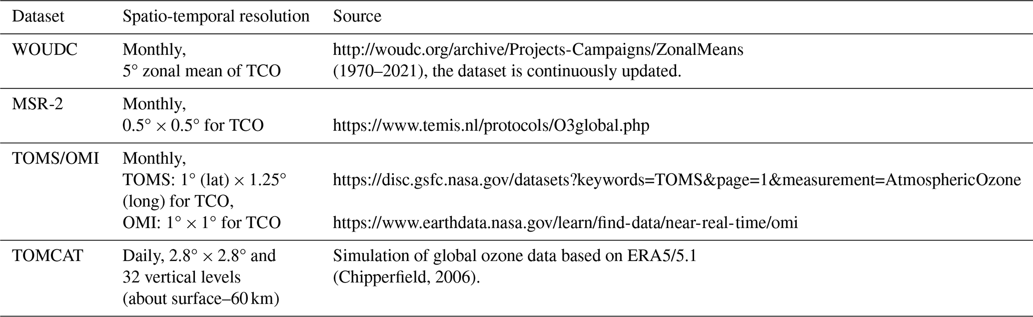
We use TCO data from the World Ozone and Ultraviolet Radiation Data Centre (WOUDC), the Multi-sensor reanalysis (MSR-2) and Total Ozone Mapping Spectrometer/Ozone Monitoring Instrument (TOMS/OMI) in this study to assess long-term Antarctic variations. In addition to these observational products, ozone profile datasets simulated by the TOMCAT global three-dimensional chemical transport model are also used to provide consistency for the analysis and to gain better insight into vertical changes. A detailed summary of the data sources and their respective spatio-temporal resolutions are shown in Table 1.

Table 1 Sources and temporal coverage of ozone datasets. The last access for all websites cited in this table: 11 June 2026.

2.1 WOUDC data

The WOUDC ground-based dataset is generated by merging measurements from Dobson and Brewer spectrophotometers along with filtered ozonometers. Zonal mean ozone values are derived using the method of calculating the “climatological” ozone deviation of stations, followed by smoothing or approximation across different stations and months to reduce uncertainty, resulting in 5° zonal averages (Fioletov et al., 2002). To ensure high data quality, the WOUDC records undergo rigorous filtering to eliminate systematic errors or unreliable results. These ground-based observations typically show excellent agreement with satellite-derived data, usually within ± 0.5 %, ensuring high consistency between the merged satellite records and the ground-based observations utilised here (Chiou et al., 2014). Antarctic ozone observations have drawn upon over 20 ground-based stations since monitoring was initiated.

2.2 MSR-2 data

The MSR-2 dataset is a comprehensive, revised ozone product constructed by merging measurements from 15 different satellite retrieval instruments. These include the TOMS series (Nimbus-7 and Earth Probe), SBUV (Nimbus-7 and NOAA-9, -14, -11, -16, -17, -18, -19), BUV-Nimbus 4, GOME (ERS-2), SCIAMACHY (Envisat), OMI (EOS-Aura), and GOME-2 (Metop-A). Systematic biases in all satellite records are first corrected using independent ground-based total ozone data from the WOUDC, accounting for factors such as solar zenith angle, viewing angle, trend, and effective ozone temperature. The final global ozone dataset is generated using data assimilation techniques based on a chemical transport model driven by meteorological fields from the European Centre for Medium-Range Weather Forecasts (ECMWF) (van der A et al., 2015).

2.3 TOMS/OMI data

The TOMS and OMI data were processed using the Version 8 algorithm developed by NASA Goddard's Ozone Processing Team (Wellemeyer et al.,  2004). The TOMS programme began in 1978 and we use TCO measurements from onboard Nimbus-7, Meteor-3, and Earth Probe. OMI, onboard the Aura satellite, continues to monitor ozone columns in the atmosphere as a continuation of the TOMS series. OMI measurements provide extremely high spatial resolution and have made significant contributions to the study of stratospheric and tropospheric chemistry (Levelt et al., 2006). Despite the overlap of time periods measured by different TOMS platforms, the bias of ozone data between them is 1 %–2 % (Kroon et al., 2008).

2.4 TOMCAT model data

TOMCAT/SLIMCAT (hereafter TOMCAT) is a three-dimensional chemical transport model (CTM) (Chipperfield, 2006) and is driven here by the ERA5/5.1 reanalysis meteorological fields provided by the ECMWF (Hersbach et al., 2020). The model uses a detailed gas-phase stratospheric chemistry scheme, including the reactions of the odd-oxygen, nitrogen, hydrogen, chlorine and bromine families. The model also has a detailed description of heterogeneous chemistry on polar stratospheric clouds (PSCs) and lower stratospheric sulphate aerosols. The model setup used here is similar to that in Zhou et al. (2024). Time-varying solar spectral irradiances are from NRL v2 (Coddington et al., 2016) that are extended until December 2023. Variations in stratospheric aerosol resulting from volcanic eruptions are represented by surface area density (SAD) fields. These fields are the same as used in CMIP6 simulations (until December 2016) and for later periods we use SAGE III measurements based on SAD data products (Knepp et al., 2024). Implementation of SAD and solar spectral irradiance (SSI) variations are described by Dhomse et al. (2015, 2016). TCO values from the model are calculated by vertical integration of these simulated ozone profiles.

3 Methods

3.1 Multiple linear regression (MLR)

Ozone trends are generally estimated using MLR, which incorporates trend terms along with proxies for known dynamical and chemical processes. Various methods have been applied to represent trend terms in the MLR, such as the independent linear trends (ILT), the piecewise linear trends (PLT), and the equivalent effective stratospheric chlorine (EESC) to account for long-term ozone changes due to variations in ODS (Harris et al., 2008; Nair et al., 2013; Chehade et al., 2014). The trend term is the only non-periodic term in the MLR, whereas other terms generally exhibit some form of period or peak. Changes in stratospheric ozone levels are driven by the combined influences of climate variability and ODS. Consequently, the net ozone trend need not strictly track EESC variations before and after the ODS peak, and ILT will better represent the ozone changes caused by other non-periodic forcings. Other terms used include the QBO, 11-year solar cycle, ENSO, AAO, BDC, stratospheric aerosol optical depth (SAOD) (Toro A et al., 2017; Weber et al., 2018, 2022). The MLR equation used here is shown in Eq. (1):

$$\begin{array}{}\text{(1)}& \begin{array}{rl}y\left(t\right)& =a_{\mathrm{1}}\cdot X_{\mathrm{1}}\left(t_{\mathrm{1}}\right)+a_{\mathrm{2}}\cdot X_{\mathrm{2}}\left(t_{\mathrm{2}}\right)+{\mathit{\alpha }}_{\mathrm{QBO}\mathrm{10}}\cdot {\text{QBO}}_{\mathrm{10}}\left(t\right)\\ & +{\mathit{\alpha }}_{\mathrm{QBO}\mathrm{30}}\cdot {\text{QBO}}_{\mathrm{30}}\left(t\right)+{\mathit{\alpha }}_{\mathrm{SAOD}}\cdot \text{SAOD}\left(t\right)\\ & +{\mathit{\alpha }}_{\mathrm{solar}}\cdot S\left(t\right)+{\mathit{\alpha }}_{\mathrm{BDC}}\cdot \text{BDC}\left(t\right)+{\mathit{\alpha }}_{\mathrm{ENSO}}\cdot E\left(t\right)\\ & +{\mathit{\alpha }}_{\mathrm{AAO}}\cdot \text{AAO}\left(t\right)+\mathit{\epsilon }\left(t\right),\end{array}\end{array}$$

where y(t) is the ozone time series and t is the year (month) during period 1979–2023, X₁(t₁) and X₂(t₂) are the linear trend before and after EESC reaches a maximum over the Antarctic. t₁ and t₂ indicate that X₁ and X₂ are only different from zero for years t before (1979–2000) and after (2001–2023) the EESC peak, respectively. Analysis of ozone data shows a turning point in the continued decline of Antarctic ozone around 2000, consistent with the EESC calculations showing a maximum in the polar regions at that time (Newman et al., 2006, 2007). We also found that choosing the turnaround year for the overall ozone trend (e.g., 2000 vs. 2001) has little impact on the trajectory (Zambri et al., 2021; Kessenich et al., 2023). To quantitatively describe the contribution of different factors on ozone, we calculated the peak contribution of the proxies to ozone and its rate of change. The contribution is given by Eq. (2):

$$\begin{array}{}\text{(2)}& \text{TCO}\left[\mathit{\%}\right]={\displaystyle \frac{max\left(X\right(t\left)\right)-min\left(X\right(t\left)\right)}{\text{mean}\left(y\right(t\left)\right)}}\times \mathrm{100}\mathit{\%}\end{array}$$

where $max\left(X\right(t\left)\right)-min\left(X\right(t\left)\right)$ represents the peak contribution, X(t) is the contribution of different factors to ozone during the period 1979–2023, and y(t) is the TCO time series.

3.2 Proxies for main impact factors

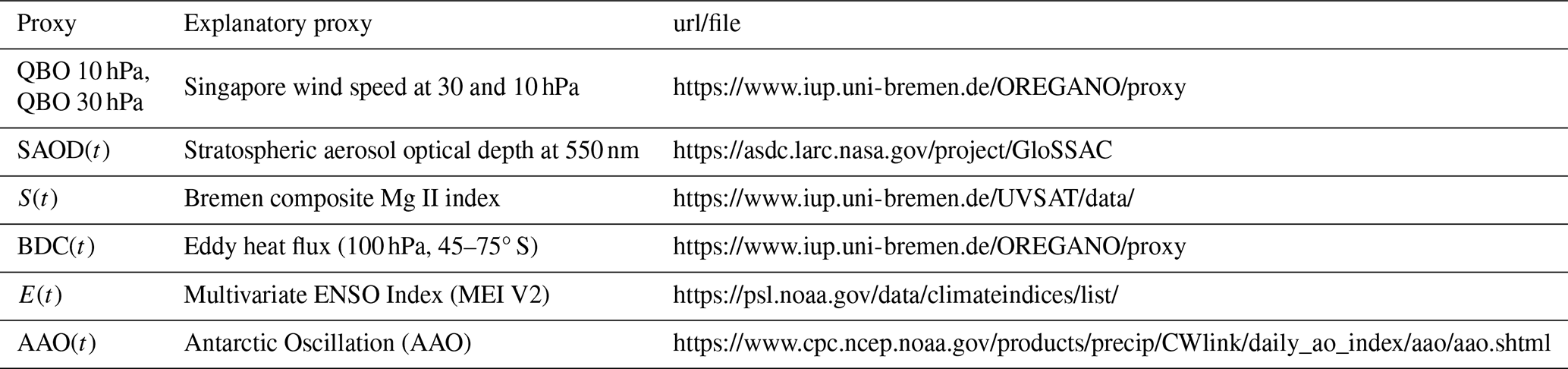
Sources of proxy data are shown in Table 2. To account for the effect of the QBO phase on ozone variability, equatorial zonal winds (10 and 30 hPa) are commonly used as indices (Chehade et al., 2014; Li et al., 2020). SAOD has been used to represent volcanic aerosol changes following eruptions such as those of El Chichón and Mt. Pinatubo, which have been shown to affect ozone in the SH (Sato et al., 1993; Aquila et al., 2013; Dhomse et al., 2015). The SAOD proxies are provided as a function of latitude, while we utilised the SH average aerosol data. To account for solar variability, a driver of long-term ozone changes, we use the Bremen composite Mg II index (Snow et al., 2014). The BDC is usually expressed as the eddy heat flux (EHF) at 100 hPa, a proxy widely used to assess dynamical influence on the interannual ozone variability (e.g. Newman et al., 2001; Dhomse et al., 2006; Weber et al., 2011). ENSO variability is also known to have significant impact on the SH stratosphere, leading to early or delayed break-up of the polar vortex (e.g. Randel et al.,  2002; Camp and Tung, 2007). Sea surface temperature (SST) trends modulate Antarctic stratospheric ozone recovery (Hu et al., 2025). Consequently, ENSO, as the dominant mode of SST variability, should be included as an impact factor. The AAO can affect ozone and is closely related to the Antarctic ozone hole through the stratospheric circulation that should be from the tropics to the polar regions (Thompson and Solomon, 2002; Frossard et al., 2013). In the MLR, AAO and BDC are represented by the mean of the autumn-to-spring accumulation, while other proxies use the monthly mean time series for monthly analyses and annual mean time series for annual analyses with no time lags.

Table 2 Sources of impact proxies in the MLR. The last access for all websites cited in this table: 11 June 2026.

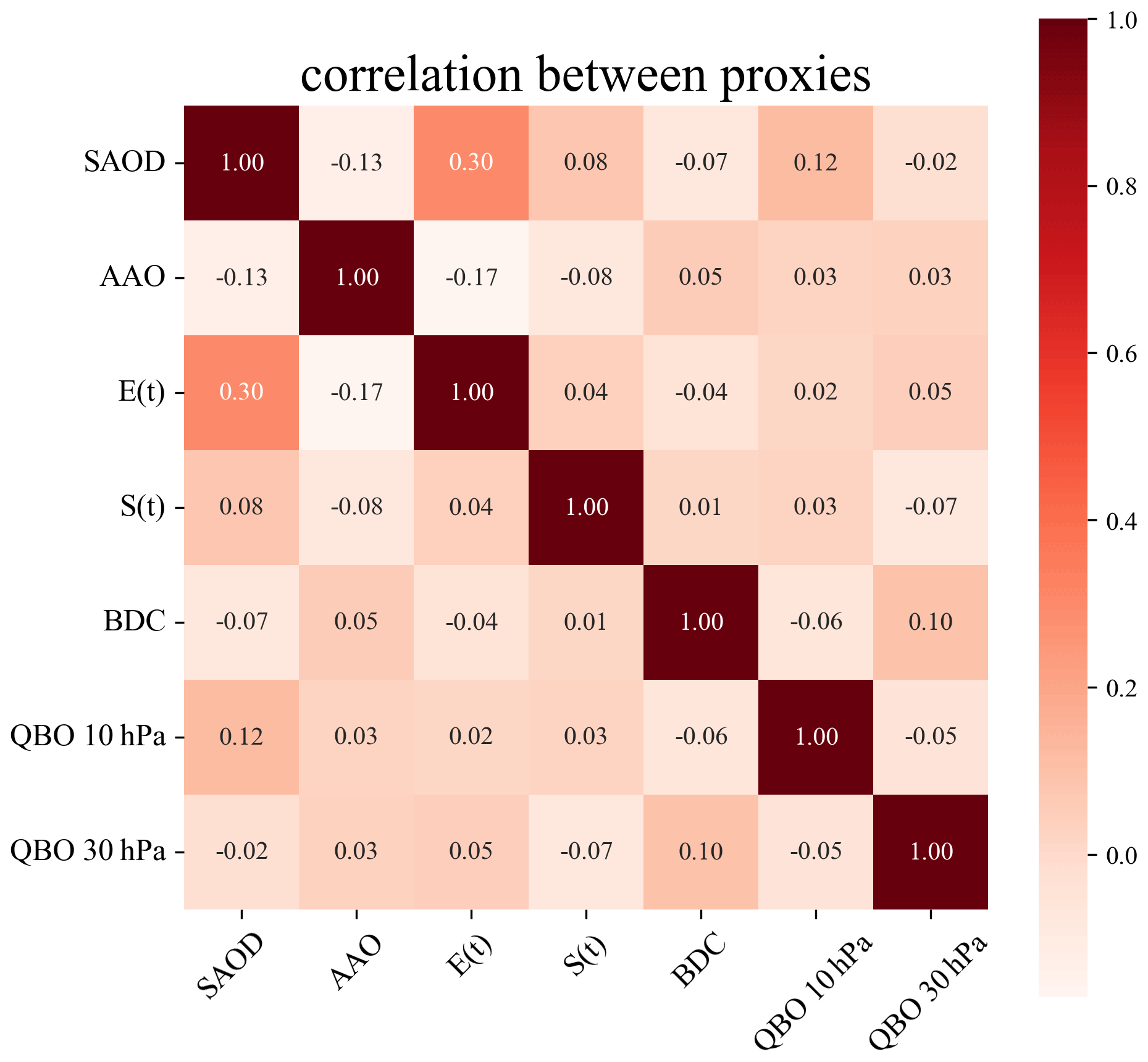
An important criterion of MLR is that the impact proxies should not be highly correlated with each other. As shown in Fig. 1, correlations between the proxies are minimal, with the highest coefficient at 0.3, satisfying the precondition for MLR analysis. Therefore, these proxies are suitable for analysing long-term ozone changes.

Figure 1 Correlation coefficients among the main MLR impact proxies.

4 Long-term trends in Antarctic ozone

Antarctic ozone recovery exhibits a strong seasonal dependence, especially in the spring. While chemical processes dominate in September, dynamical factors exert greater control in October (Strahan et al., 2014; Solomon et al., 2016; Stone et al., 2021). Figure 2 illustrates the long-term ozone trends in the wider Antarctic polar cap (60–90° S) from four datasets, reflecting the persistence of the deep ozone hole and extended periods of low ozone over Antarctica during 2020–2023. Among these, WOUDC data indicate relatively small fluctuations in TCO values. In contrast, the TOMCAT and MSR-2 exhibit more pronounced variations. To ensure consistency across datasets with different temporal coverage, trends were analysed for 2001–2023. During this period, the trends are not statistically significant, with September close to zero and October exhibits a decline of approximately −1 DU yr⁻¹. Overall, the ozone variations among the datasets show good consistency and we examined trends across different time spans to clarify these seasonal behaviours.

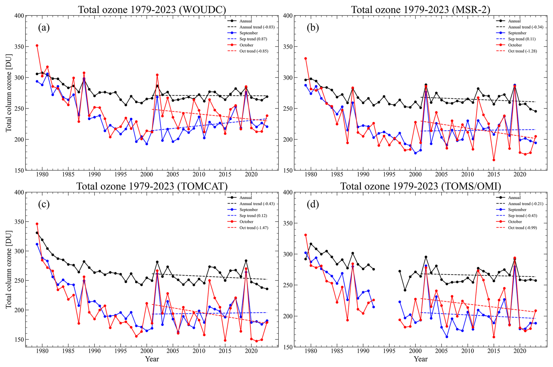
Figure 2 The TCO time series (DU) in the Antarctic (60–90° S) from multiple datasets. (a) WOUDC, (b) MSR-2, (c) TOMCAT, and (d) TOMS/OMI. The black line represents the annual mean time series, the blue line represents the September time series, and the red line represents the October time series. The dotted lines show the linear trends (DU yr⁻¹) from 2001 to 2023, corresponding to the annual mean (black), September (blue), and October (red).

Table 3 summarizes the independent linear trends from the four datasets over different time periods along with MLR correlation coefficients (R²). For the period 1979–2000, annual TCO declined at 2–3 DU yr⁻¹, with a more pronounced decline of 5–6 DU yr⁻¹ during September and October. None of the post-2001 trends are statistically significant at the 2σ level. The long-term annual trend from 2001 to 2019 was approximately 0.4 DU yr⁻¹ across multiple datasets, whereas the trend was negative (∼ −0.3 DU yr⁻¹) for the period 2001–2023. September exhibits consistently positive trends for 2001–2019. However, anomalously low ozone levels persistently observed during 2020–2023 attenuated the trends from 2001 to 2023, bringing them closer to zero. October trend estimate shifts from weakly positive (e.g. 0.3 ± 3.2 DU yr⁻¹ for 2001–2019 for TOMCAT) to negative (−1.5 ± 2.4 DU yr⁻¹ for 2001–2023). This shift suggests that EESC might not accurately reflect the ozone changes in October. Furthermore, the decline in the trends in September and October on lengthening the data record are similar, indicating that other factors (e.g. BDC) have become more important for spring ozone depletion under ODS controls.

Table 3 Independent linear trends (DU yr⁻¹) of TCO in the annual mean, September, and October means for different time spans for four datasets, and the correlation between each dataset and MLR (R²). Numbers in parentheses are the 2σ trend uncertainty.

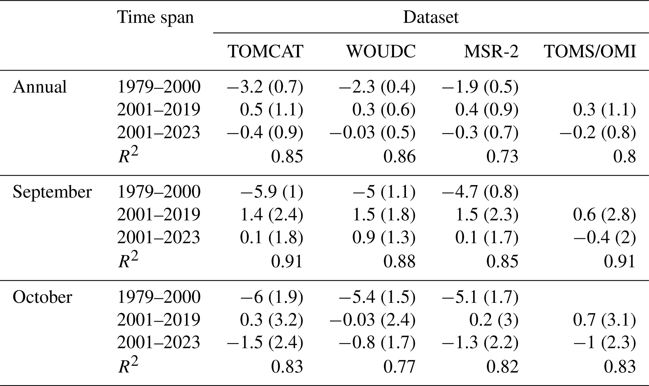
To further evaluate the ability of the regression framework to reproduce the observed variability, we examine the TOMCAT-based MLR results in detail. Figure 3 presents the time series of TCO and the MLR based on the TOMCAT dataset. The results generally suggest a post-2000 decline, with an annual trend of −0.4 ± 0.9 DU yr⁻¹ and a stronger October trend of −1.5 ± 2.4 DU yr⁻¹ through 2023. In September, the TOMCAT trend was very slightly positive, while the trend estimated by the TOMCAT-based MLR was negative (−0.7 DU yr⁻¹). Regression analysis across four datasets demonstrates good agreement in the long-term ozone changes. The R² values in Table 3 indicate that the independent variables in the MLR models effectively reproduce the ozone time series for each dataset. The independent variables in the MLR can explain about 85 % of the variance in the interannual time series. Among these datasets, the MLR of TOMCAT accurately reproduced simulated long-term ozone variability, explaining 91 % of the variance in the September time series in particular.

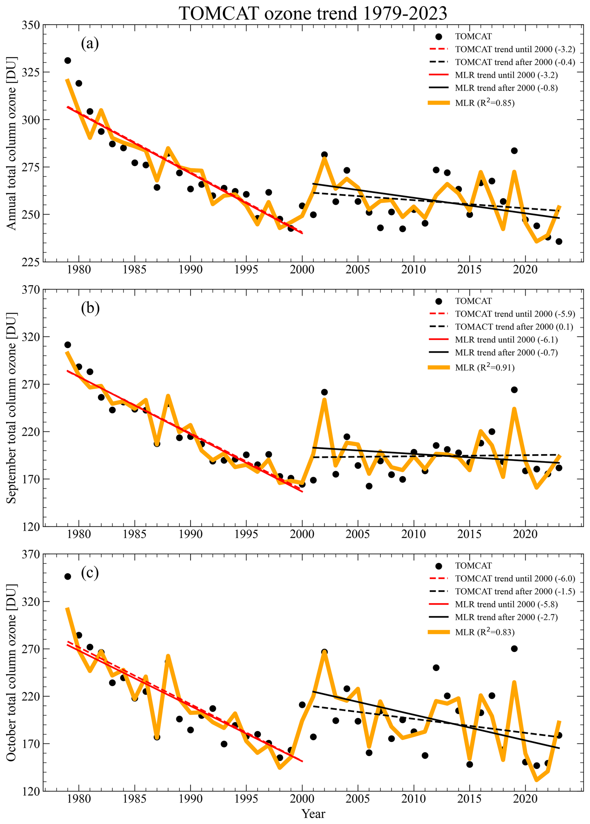
Figure 3 TCO time series (DU) of the TOMCAT dataset from 1979 to 2023. (a) Annual mean, (b) September mean, and (c) October mean. The black dots are TOMCAT, the orange thick line is the time series based on MLR results, the red lines are the linear trends from 1979 to 2000 (dashed TOMCAT, solid MLR), and the black lines are the linear trends from 2001 to 2023.

To determine whether the September–October contrast arises from changes at specific altitudes, we examined vertical ozone trends in the austral winter/spring. Kessenich et al. (2023) effectively analysed the daily variations of ozone concentration in the polar regions during spring and winter based on Aura Microwave Limb Sounder data. Ozone mixing ratios from the TOMCAT dataset were analysed as a function of altitude and day of the year (1 August–10 November) for 2001–2023 (Fig. 4). In August, the ozone mixing ratio trend at 1 hPa showed a negative change which gradually extended downward. By September, this trend reached the mid-stratosphere, resulting in a negative anomaly, with a rate of change in the ozone mixing ratio of −0.03 parts per million per year (ppmv yr⁻¹). However, positive trends dominate the upper and lower stratosphere, reaching ∼ 0.04 ppmv yr⁻¹, exceeding the magnitude of the negative changes and consistent with the recovery observed in September. In October, a broader negative region emerged (5–80 hPa), peaking at −0.07 ppmv yr⁻¹ and coinciding with the main Antarctic ozone layer (4–20 hPa). The persistent negative trend in ozone continued into early November, suggesting prolonged low Antarctic ozone values and demonstrating the need for continued monitoring of dynamical and chemical processes driving these trend changes.

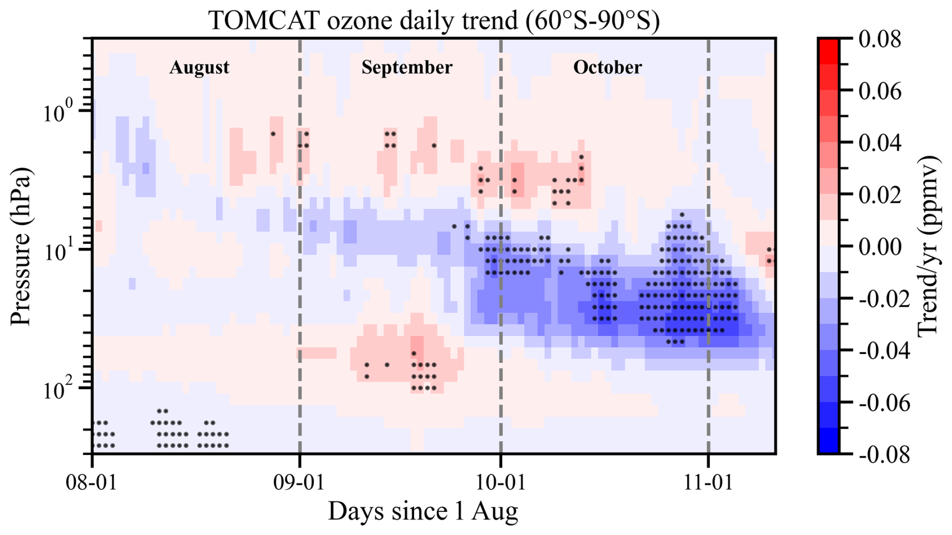
Figure 4 Vertical cross section of daily trends (2001–2023) in ozone volume mixing ratio (ppmv yr⁻¹) from TOMCAT. Trends are shown for 1 August to 10 November (2001–2023). Stippled areas are statistically significant above the 95 % confidence level.

To elucidate the impact of each proxy, we analyse their contributions to ozone variation using the MLR results of the TOMCAT dataset. Based on Eq. (2), we evaluated the peak contribution of each proxy to TCO (Fig. 5). BDC dominates the interannual variation of ozone, while the contribution of combined QBO accounts for up to 5.5 % of the long-term variability. The dominant role of the BDC can be explained by its transport of ozone from the tropical source region to high latitudes, with ozone accumulation reaching a maximum at mid to high latitudes from May to September. The efficiency of transport depends on the strength of BDC (Weber et al., 2011; Fioletov et al., 2023). These winter/spring transport processes lead to a more pronounced contribution of the BDC to the long-term ozone variability in September and October, with the peak rate reaching 51 %, indicating its significant impact on Antarctica TCO fluctuation. After a volcanic eruption, SAOD will remain enhanced in the stratosphere for a limited period. SAOD exerted a significant influence on Antarctic ozone following the El Chichón (1982) and Mt. Pinatubo (1991) volcanic eruptions, with the peak rate reaching 10.1 %. Comparatively, peak contributions of QBO and solar cycle are approximately 8 % in September, whereas other proxies contribute less than 6 %.

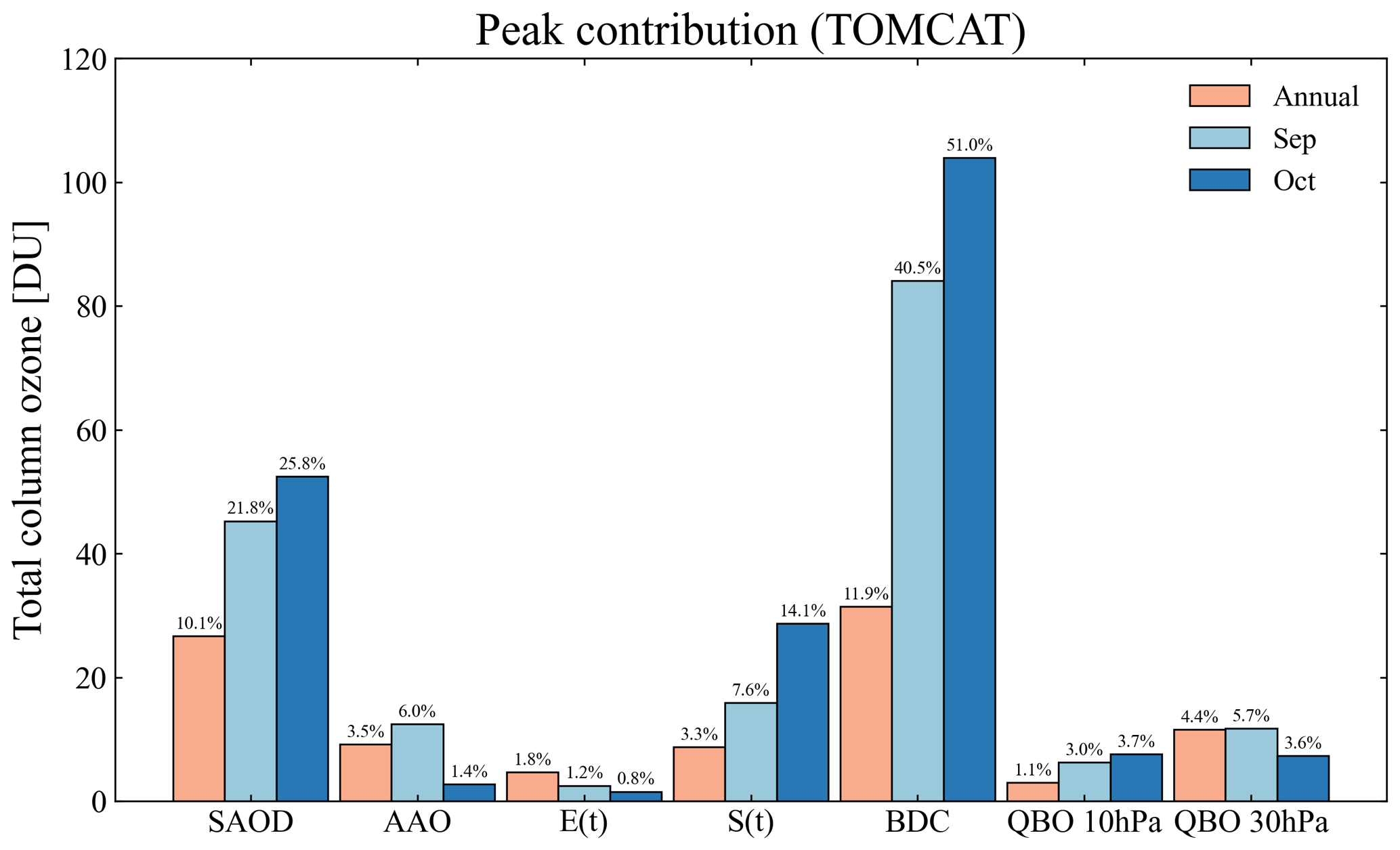
Figure 5 Peak contribution (DU) of each proxy in the MLR to TCO changes from 1979 to 2023 based on TOMCAT. Orange: annual mean; light blue: September; blue: October. The magnitude of peak contribution in percent is labelled above each bar.

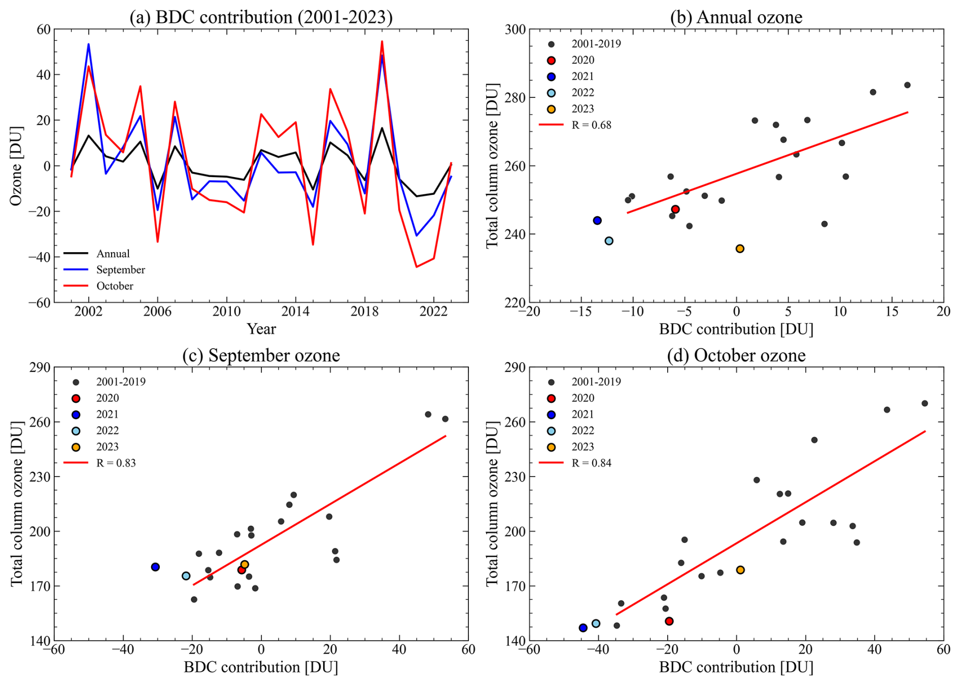
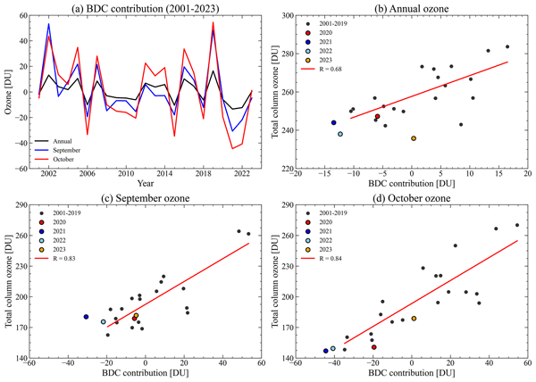
Figure 6 (a) BDC contribution to TCO changes (DU) from 2001 to 2023 for the annual, September, October means. Correlation between the BDC contribution and TCO for (b) annual mean, (c) September, and (d) October over Antarctica during 2001–2023. The recent period (2020–2023) is highlighted in colour, while the earlier years are shown in black.

During the austral winter/spring, the MLR well described the contribution of dynamic processes to stratospheric ozone, with BDC being the main driver of interannual ozone variation and an important contributor to long-term changes. Figure 6 shows this contribution of BDC to TCO changes from 2001 to 2023. BDC has a significant impact on the recent ozone variability, contributing up to −45 DU in October during 2020–2023. Figure 6b–d demonstrates a positive correlation between TCO changes and the contribution of BDC from 2001 to 2023, with the correlation coefficient reaching 0.84 in October. Notably, the low ozone levels observed in 2021–2022 coincided with negative BDC contributions. Although TCO remained relatively low in 2023, the corresponding BDC contribution was small.

5 Model sensitivity simulations

5.1 Setup of the model experiments

Figures 5 and 6 clearly show that variations in BDC strength have a profound impact on Antarctic ozone recovery. To investigate this further, we performed simulations using TOMCAT to explore the modulation effect of BDC on ozone. The control experiment (CRL) uses the standard chemical and dynamical parameters spanning the period 2001–2023. To assess the impact of BDC intensity, two sensitivity experiments were conducted based on typical years of BDC anomalies: S2002 represents a year with strong BDC (2002), while S2006 represents a year with weak BDC (2006). In these experiments, wind forcing and temperature from 2001 to 2023 were altered to modify BDC intensity, while other parameters remained unchanged. The experimental design is summarised in Table 4.

Table 4 Design of TOMCAT sensitivity experiments.

The selection of 2002 and 2006 was guided by interannual variation of ozone and ODS changes to ensure that the BDC intensity is the dominant factor influencing the ozone variation. Previous studies have shown a weakening of ozone transport to the polar regions in 2006, accompanied by persistent cold temperatures and stable polar vortex in late winter and early spring (Peshin, 2008; Grytsai, 2011). In contrast, the typical strengthening of BDC occurred in 2002 as a result of unusually strong upward planetary wave propagation. Elevated stratospheric temperature in the SH, along with polar vortex splitting, created an unfavourable environment for polar ozone depletion (Allen et al., 2003; Sinnhuber et al., 2003). These marked differences in circulation intensity highlight the contrasting dynamical regimes of 2002 and 2006, making them ideal case studies for examining the role of BDC in Antarctic ozone variability.

5.2 Simulation results

An increase in TCO is observed in S2002 (strong BDC; Fig. 7), with values from 2001 to 2023 approximating those in 2002. Conversely, S2006 (weak BDC) reveals ozone reductions, with September and October ozone values resembling those in 2006. The sensitivity experiment results suggest that the peak contribution rates are consistent with the MLR results, with the annual mean and October peak contribution rates of ∼ 15 % and ∼ 52 %, respectively. Despite Antarctic ozone trends showing a decline during 2001–2023 in the annual and October means, both S2002 and S2006 exhibited positive trends after controlling for BDC intensity, with notable consistency between the two experiments. This positive trend corresponds to the changes in EESC, providing further evidence that the reduction of ODS is driving the expected recovery of the Antarctic ozone layer.

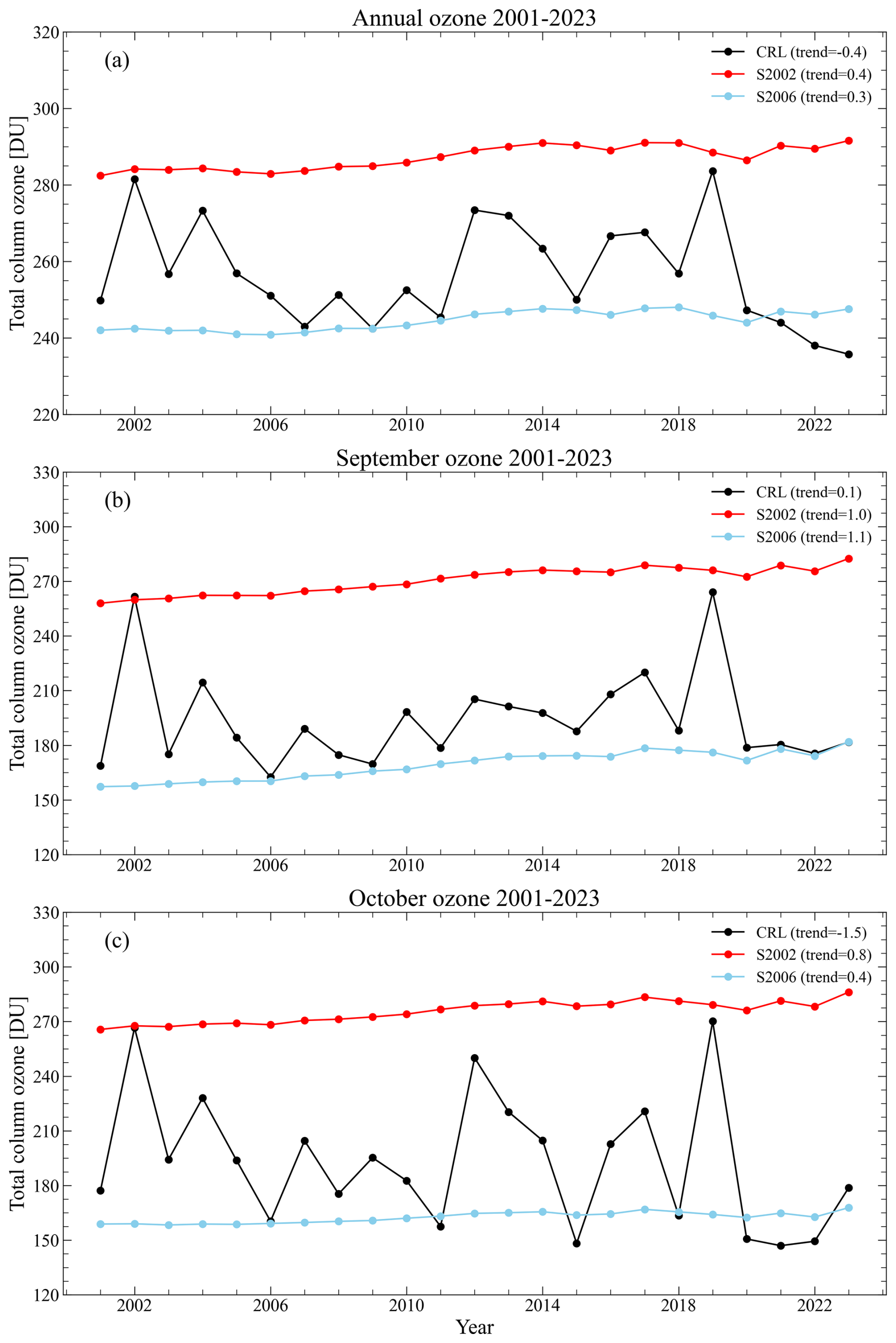
Figure 7 TCO (DU) changes in Antarctica for TOMCAT control and sensitivity experiments from 2001 to 2023. (a) Annual mean, (b) September, and (c) October. Black: CRL, red: S2002 (strong BDC), sky blue: S2006 (weak BDC).

Monthly TCO for the control and sensitivity experiments from 2001 to 2023 are shown in Fig. 8. Ozone typically experiences pronounced depletion in September, with TCO dropping below 220 DU, a threshold associated with the formation of the ozone hole. TCO values dropped to approximately 150 DU in October–November during 2020–2022, significantly lower than in most years of the 2001–2019 period. Despite springtime exhibiting improvement in 2023 (TCO ∼ 180 DU), persistently low levels throughout the year resulted in a suppressed annual mean. According to simulation S2002, enhanced circulation during the winter and spring increased TCO towards the values of 2002. With the BDC intensity held constant, Antarctic spring ozone exhibits substantial interannual variability (up to 30 DU). Nevertheless, ozone levels in recent years (2020–2023) are significantly elevated compared with most of the past 2 decades.

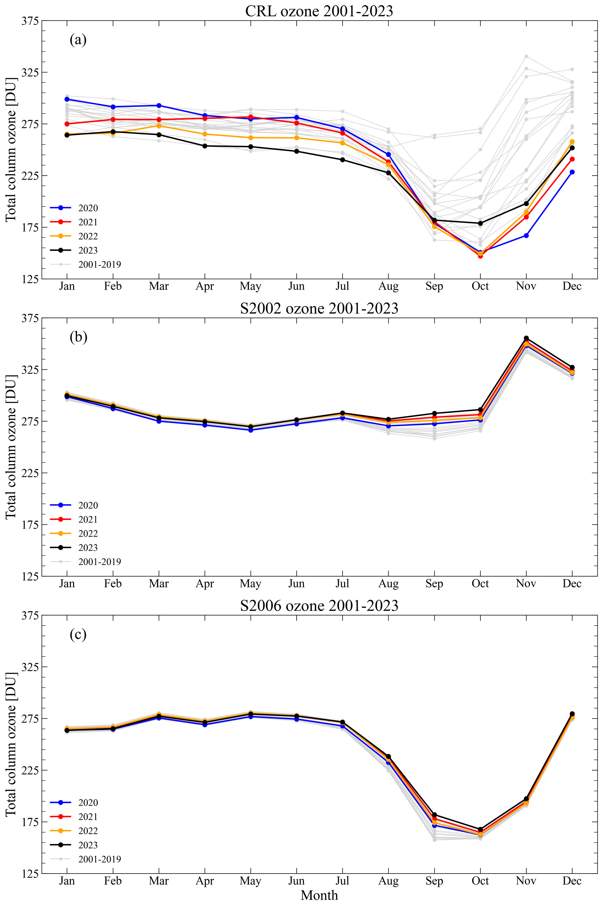
Figure 8 Monthly TCO (DU) in the Antarctic for TOMCAT control and sensitivity experiments from 2001 to 2023. The years 2020 to 2023 are highlighted in colour. (a) CRL, (b) S2002, and (c) S2006.

Figure 9a shows the monthly mean temperature at 50 hPa from 2001 to 2023. The cooler temperatures in the winter and especially the spring from 2020 to 2022 were associated with the persistently low ozone values. The temperature anomaly is inextricably linked to BDC strength and the timing of vortex breakup (Weber et al., 2011; Butchart, 2014). As shown in Fig. 9b, EHF was high in the spring during 2020–2022, indicating the weakened circulation and reduced ozone transport from the tropics to the polar regions. The higher springtime temperature and EHF in 2023, compared with the springs of 2020–2022, contributed to the elevated ozone concentrations (Fig. 8a).

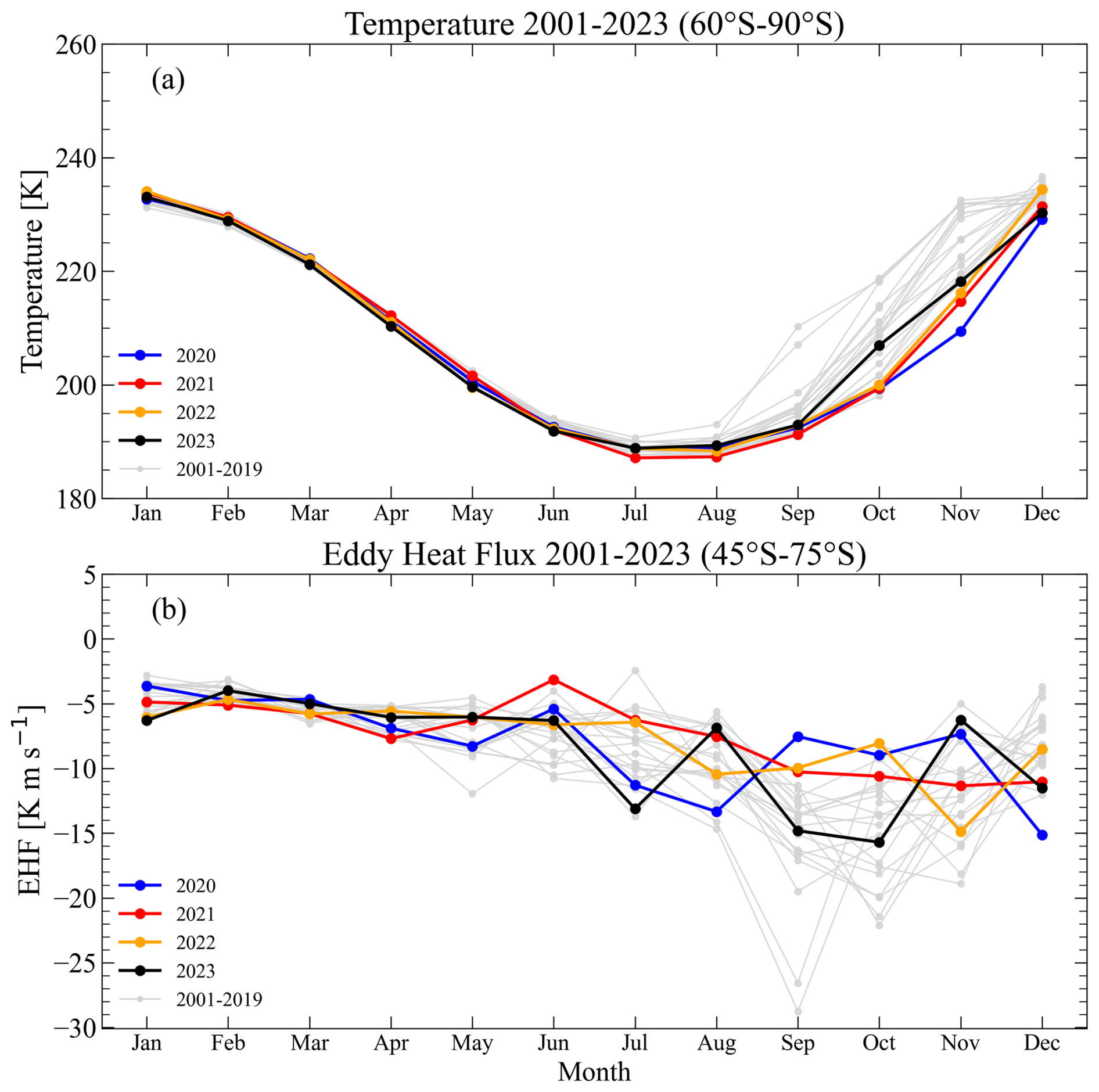
Figure 9 (a) Monthly mean temperature (K) at 50 hPa (60–90° S) in Antarctica from 2001 to 2023. The years 2020 to 2023 are highlighted in colour. (b) Monthly mean eddy heat flux (EHF) (K m s⁻¹) at 100 hPa (45–75° S) from 2001 to 2023.

6 Summary and conclusions

This study combined satellite-based observations, reanalysis datasets as well as chemistry-transport model simulations to analyse the long-term ozone trend over Antarctica during 1979–2023. Using MLR, we analysed the contributions of dynamical and chemical proxies to ozone variability. Furthermore, based on the TOMCAT 3-D model, we conducted sensitivity experiments to investigate the impact of the BDC on ozone. Our main conclusions are:

• 1.

  Multiple datasets can consistently well represent the long-term ozone changes over Antarctica. Over the period 2001–2019 annual mean ozone showed signs of recovery, but the persistent low ozone values from 2020 to 2023 resulted in the trend in annual ozone shifting downward to −0.4 ± 1.1 DU yr⁻¹ during 2001–2023.

• 2.

  For the 2001–2019 period, TCO trends across multiple datasets were approximately 1.5 and 0.3 DU yr⁻¹ in September and October, respectively. Over the extended 2001–2023 period, WOUDC trends were positive in September (0.9 ± 2.4 DU yr⁻¹) and negative in October (−0.8 ± 2.4 DU yr⁻¹). MSR-2 and TOMCAT trends were close to zero but remained marginally positive (0.1 ± 1.8 DU yr⁻¹) in September, whereas October declined at approximately 1.5 DU yr⁻¹.

• 3.

  The MLR using multiple datasets effectively captures the long-term ozone variations over Antarctica. Among these datasets, the MLR based on the TOMCAT output performed better, explaining 91 % of the variance in the time series in September. The daily ozone trends based on the TOMCAT dataset during the period 2001–2023 showed that the recovery of ozone in September is due to increasing ozone in the lowermost stratosphere. In contrast, in October, negative trends are observed in the entire lower stratosphere. This seasonal contrast explains why the TCO trends are negative in October but slightly positive in September.

• 4.

  Proxy analysis highlights the dominant role of the BDC in the Antarctic spring, and BDC contributions to ozone changes exhibited a positive correlation with TCO during 2001–2023. Despite SAOD contributing about 10 % to long-term ozone interannual variability, this signal was largely driven by the elevated aerosol loading following the Mt. Pinatubo (1991) volcanic eruption. Other proxies also exert smaller but non-negligible contributions to the ozone change.

• 5.

  Sensitivity experiments further reveal that the strengthening (weakening) of the BDC led to an increase (decrease) in the transport of tropical ozone to the polar regions. The BDC anomaly in the SH significantly affects the polar temperature, and thereby ozone depletion, with peak contribution of circulation anomalies to long-term ozone changes reaching 51 % in October.

Overall, in the long-term, the evolution of Antarctic ozone reflects the interplay of multiple processes, with dynamical drivers exerting a particularly strong influence on recovery patterns. Perturbations to the BDC play a substantial role in the long-term ozone trend, requiring further research and continued attention to the ozone hole and dynamical processes. This will improve our understanding of long-term ozone variability and ability to predict future changes in the Antarctic ozone hole.