Aircraft-derived particle fluxes distinguish entrainment zone and decoupled layer nucleation in marine boundary layers

The vertical distribution of freshly nucleated aerosol particles in the marine boundary layer remains poorly constrained, limiting our ability to represent new particle formation in climate models. Here we characterize 3–10 nm particle events, termed small particle events (SPEs), by deriving their vertical turbulent fluxes from aircraft measurements during the Aerosol and Cloud Experiments in the Eastern North Atlantic (ACE-ENA) campaign. To overcome stationarity limitations of traditional eddy covariance methods, we applied continuous wavelet transform analysis to data collected during June–July 2017 and January–February 2018 flights over the Azores. Our flux-based analysis revealed two distinct SPE scenarios with different vertical structures and spatial extents. The first featured nucleation in the entrainment zone, where free tropospheric air entrains into the boundary layer. The second showed nucleation in the decoupled layer, a stratified region between the well-mixed surface layer and cloud-topped upper boundary layer. In both cases, convergence of air masses from different layers diluted preexisting aerosol surface area to very low levels, creating conditions favorable for nucleation and generating strong downward particle fluxes. SPEs occurred in 15 % of flights, challenging prevailing theoretical expectations that new particle formation should rarely occur in marine boundary layers due to high condensation and coagulation sink capacity of sea spray aerosols. Aircraft-derived particle fluxes provide first observational constraints on the vertical location and source strength of likely nucleation regions in the remote marine boundary layer, improving aerosol source representations in climate models and reducing uncertainties in aerosol-cloud interactions.

1 Introduction

Cloud adjustments due to aerosols constitute one of the most significant uncertainties in climate modeling (Intergovernmental Panel on Climate Change (IPCC), 2023). The magnitude of anthropogenic aerosol radiative forcing over the industrial period is strongly influenced by the abundance and properties of natural aerosols (Andreae, 2007; Carslaw et al., 2013; Hoose et al., 2009; Meskhidze et al., 2011). While uncertainties in aerosol radiative forcing from different processes (emissions, long-range transport, new particle formation, and removal) vary spatially, marine boundary layer (MBL) cloud microphysical properties exhibit the highest sensitivity to aerosol changes (Bellouin et al., 2020; Zhang et al., 2024). Understanding how marine low level clouds and their radiative effects respond to changing aerosol load is important due to their extensive spatial coverage, low optical thickness, and low background cloud condensation nuclei (CCN) concentrations. The response of these clouds to changes in aerosol loading remains poorly constrained and represents a key source of uncertainty in climate projections (Zhang et al., 2024). Consequently, understanding aerosol composition, dynamics, and the mechanisms controlling CCN number budgets within the MBL is critical for improving climate models and reducing predictive uncertainties. While freshly nucleated particles in the 3–10 nm size range must undergo substantial growth before reaching CCN-relevant sizes (>50–80 nm), this growth pathway is well established in marine environments. At typical marine boundary layer growth rates of 1–3 nm h⁻¹ (Ehn et al., 2010; Nieminen et al., 2018; O'Dowd et al., 2010; Zheng et al., 2018), newly formed particles can reach CCN sizes within 24–48 h. This timescale is consistent with air mass residence times in the remote marine boundary layer (Kulmala et al., 2012; Zheng et al., 2021). Constraining the vertical location and flux magnitude of freshly nucleated particles therefore represents a critical first step toward understanding the full aerosol number budget in marine environments, including the ultimate contribution of NPF to CCN populations.

Previous studies have identified three primary aerosol sources in remote MBLs: (1) long-range continental transport (Logan et al., 2014), (2) downward mixing of particles formed in the free troposphere (FT) through new particle formation (NPF) mechanisms (Clarke et al., 2013), and (3) sea spray emissions (Quinn et al., 2017). NPF occurring either near the top of stratocumulus cloud decks within open-cell regions (Petters et al., 2006) or in the upper portions of mid-latitude MBLs (Zheng et al., 2021) has been suggested as an important in-situ aerosol source within the MBL. However, the difficulty in capturing actual nucleation events and determining their precise vertical location has led to the prevailing theoretical view that NPF should rarely occur in remote marine boundary layers over open oceans. This expectation is based on the high condensation and coagulation sink capacity of the remote MBL, which includes not only sea spray aerosols (Bates et al., 1998; Pirjola et al., 2000) but also accumulation-mode sulfate and organic particles entrained from the free troposphere (Yoon and Brimblecombe, 2002). Clouds further suppress NPF by scavenging Aitken-mode particles (Zheng et al., 2018), accelerating sulfate production on existing droplets through aqueous-phase SO₂ oxidation (Sanchez et al., 2021), and sequestering DMS oxidation products such as Hydroperoxymethyl thioformate (HPMTF) that would otherwise contribute to sulfuric acid formation (Novak et al., 2021). Independent corroboration of in-situ NPF over the eastern North Atlantic comes from the Azores Stratocumulus Measurements of Radiation, Turbulence and Aerosols (ACORES) campaign, which conducted helicopter-borne observations over Graciosa Island in July 2017, overlapping in time and location with the ACE-ENA campaign analyzed here. Siebert et al. (2021) reported frequent burst-like freshly nucleated particle events near the stratocumulus cloud top and in the free troposphere, while also noting that these particles did not grow to CCN-relevant sizes within the ∼2 h observation window. This outcome is expected given the 24–48 h growth timescales discussed above. These concentration-based observations, however, could not determine the precise vertical location of the nucleation source regions, motivating the flux-based approach developed in the present study.

Determining the vertical origin of freshly nucleated particles, whether from the free troposphere, the interfacial layer near the marine boundary layer–free troposphere boundary, or the interface between the well-mixed marine boundary layer and decoupled layer, has critical implications for both fundamental understanding and climate modeling. Knowledge of where nucleation occurs is essential for understanding aerosol formation mechanisms and enabling climate models to accurately simulate aerosol number size distributions required for radiative calculations. Most atmospheric models have historically assumed that nucleation should be negligible in marine boundary layers, instead predicting that particle formation would be favored at high altitudes where both temperature and aerosol surface area are substantially lower. However, traditional time-averaged aerosol concentration measurements from aircraft campaigns provide limited information about the precise vertical location where nucleation events occur. This limitation has prevented definitive identification of nucleation zones within the marine boundary layer and hampered efforts to constrain the relative importance of different aerosol sources to marine aerosol budgets. Without direct observational evidence of where particles form, climate models continue to rely on theoretical assumptions that may not accurately represent actual nucleation processes in marine environments.

To address this critical knowledge gap, vertical turbulent flux measurements of freshly nucleated 3–10 nm particles have emerged as particularly valuable tools for inferring the vertical location of likely nucleation source regions (Islam et al., 2022). The flux direction provides indirect evidence of the likely nucleation location: positive (upward) fluxes indicate nucleation below the aircraft, while negative (downward) fluxes suggest nucleation above the aircraft. This approach offers unprecedented spatial and temporal resolution for identifying nucleation zones that cannot be detected through conventional concentration measurements alone. In this study, we derive vertical turbulent fluxes of 3–10 nm particles using data collected during the Aerosol and Cloud Experiments in the Eastern North Atlantic (ACE-ENA) campaign. The campaign comprised two intensive operational periods (IOPs) – summer 2017 and winter 2018 – utilizing the G1 research aircraft from the DOE Atmospheric Radiation Measurement (ARM) program. By applying continuous wavelet transform techniques to high-frequency aircraft measurements, we provide the first flux-based observational constraints on the vertical distribution of likely NPF source regions in remote marine boundary layers, enabling improved representation of aerosol sources in climate models.

2 Materials and methods

2.1 Sampling site

The Department of Energy Atmospheric Radiation Measurement (DOE–ARM) Eastern North Atlantic (ENA) facility is positioned on Graciosa Island within the Azores archipelago, located in the northeastern Atlantic Ocean to the west of Portugal (Mather and Voyles, 2013). Air mass transport to this location follows four main pathways: (1) polluted outflow from North American sources, (2) continental emissions originating from northern European regions, (3) relatively clean Arctic air masses, and (4) air masses that recirculate within the Azores High pressure system (Wood et al., 2015; Zheng et al., 2018). The location is characterized by a low average annual aerosol optical depth (AOD) of 0.12 (Logan et al., 2014).

Data collection for this research occurred during the ACE-ENA field campaign, which included two intensive observation periods (IOPs): the initial period ran from 21 June to 20 July 2017, while the second period extended from 15 January to 18 February 2018 (Wang et al., 2019). All data from the ARM ENA site are publicly accessible through the ARM Data Discovery tool.

2.2 Instrumentation

This study utilized datasets from the ARM Aerial Facility (Schmid et al., 2014). The G-1 research aircraft was equipped with over 50 instruments for comprehensive measurements of aerosols, clouds, and atmospheric processes. Detailed information regarding flight patterns executed during the campaign can be found in Wang et al. (2019).

Two Condensation Particle Counters (CPCs, models 3025A and 3772, TSI Inc.) with nominal 50 % counting efficiency cutoff diameters of 3 and 10 nm, respectively, sampled through an isokinetic inlet exhibiting >90 % efficiency for particles with aerodynamic diameters below 5 µm. The concentration of 3–10 nm sized particles was calculated as the difference between these CPC measurements and is denoted as N₃₋₁₀ throughout this paper. Since the measurements did not extend to particle sizes small enough to directly identify nucleation events, we follow Islam et al. (2022) in using the term “small particle event” (SPE) to characterize these observations. The CPC 3772 operated at a constant 1 L min⁻¹ flow rate maintained by an external pump and critical orifice (Fan and Pekour, 2018), while the CPC 3025A sample flow rate was not actively controlled. Both flow rates remained stable across the sampling altitude range (Zheng et al., 2021). The airborne CPC configuration was validated for operation up to 4000 m altitude and across ambient relative humidity conditions of 0 %–90 % RH. For a typical polluted environment (∼5000 cm⁻³), CPC concentration measurements had an accuracy of 0.3 % (Kuang and Mei, 2019). All data used in this study passed instrument mentor specified quality control filters, which are distributed alongside the data.

Vertical wind speed (w) was measured using the Aircraft Integrated Meteorological Measurement System probe (AIMMS-20, Aventech Research Inc.). The raw measurements define downward movement as positive; therefore, the sign was inverted to align with meteorological convention (positive values indicating updrafts and negative values indicating downdrafts). Although measurements were recorded at 20 Hz, they were downsampled to 1 Hz to match the temporal resolution of the CPC data acquisition.

Aerosol size distributions from 10 to 600 nm were characterized using a Fast Integrated Mobility Spectrometer (FIMS) (Kulkarni and Wang, 2006a, b). The FIMS provides size distribution measurements at 1 s temporal resolution suitable for detecting both remote continental and clean marine aerosol concentrations, as demonstrated in aircraft-based deployments (Kulkarni and Wang, 2006a, b; Olfert et al., 2008). Particles are charged within the instrument and separated by electrical mobility using an applied electric field. The separated particles are subsequently grown into supermicron droplets in a condenser and imaged with a high-speed camera. This approach enables the FIMS to deliver size distribution measurements comparable to those of Scanning Mobility Particle Sizers (SMPS), but at a significantly higher time resolution. This study employed an advanced FIMS configuration utilizing a spatially varying electric field that extends the measurement range from 10 to 600 nm (Wang et al., 2017b, a). Size distribution measurements were normalized to dry conditions; therefore, reported size distributions and number concentrations do not represent ambient humidity conditions. Cloud contamination filters were applied to prevent misclassification of cloud droplets as aerosol particles, with detailed filtering procedures described in the following section. FIMS-derived number concentration also served as a quality control flag for the CPC 3772. Since both instruments share an overlapping detection size range (10–600 nm for FIMS; >10 nm for CPC 3772), their total number concentrations should be broadly comparable, with CPC showing a higher total number concentration than FIMS under normal operating conditions, as the CPC detects all particles above 10 nm while FIMS is bounded at 600 nm. The histogram of differences between CPC and integral FIMS concentrations (Fig. S1 in the Supplement) shows a distribution sharply peaked near zero with a slight negative skew, confirming good agreement during normal operation. The dashed red line indicates zero difference, below which CPC concentrations are physically implausible given the instruments' overlapping but non-identical size ranges. The negative tail reflects episodic periods when the CPC concentration was found to be suspect, likely due to working fluid depletion or a change in flow rate controlled by a critical orifice, producing sustained negative deviations that are physically implausible given the instruments' overlapping size ranges. These episodic malfunctions are distinct from the instrument's typical 0.3 % measurement accuracy under stable conditions (Kuang and Mei, 2019). Hence, a conservative threshold was set with CPC concentrations falling below 10 % of the simultaneously measured FIMS concentration, indicating a physically implausible discrepancy inconsistent with real atmospheric variability, and were therefore excluded from analysis as likely instrument malfunctions.

A two-dimensional stereo probe (2D-S) was used to retrieve drizzle concentration. It uses shadowgraphy to measure size distribution of hydrometeor particles in the size range 15 µm to 2.5 mm (Glienke and Mei, 2019). All data products are publicly available through the ARM DOE website with citations in the data availability section and have undergone quality control by instrument mentors. Additional technical details are available in the corresponding citations.

2.3 Data reduction

2.3.1 Droplet shattering and cloud contamination

Droplet shattering represents a significant source of measurement contamination in airborne aerosol sampling studies. Weber et al. (1998) described this phenomenon as the fragmentation of cloud droplets during in-cloud measurements, which can produce artifacts as small as 3 nm that appear in sampling instruments. Similarly, Korolev and Isaac (2005) documented comparable shattering effects with ice particles. While a detailed examination of the physical mechanisms behind droplet shattering lies beyond this study's scope, it is essential to filter such artifacts from our dataset to prevent misidentification of SPEs.

Cloud contamination was systematically detected and eliminated by calculating liquid water content (LWC) using the approach of Zheng et al. (2021), which utilizes droplet size spectra from the Fast Cloud Droplet Probe (FCDP). Visual data examination established a detection threshold of $\mathrm{3}\times {\mathrm{10}}^{-\mathrm{3}}$ g m⁻³, comparable to the 10⁻³ g m⁻³ threshold employed by Zheng et al. (2021). Data exceeding this LWC threshold were excluded from analysis.

2.3.2 Time lag correction

Accurate temporal alignment between the vertical wind speed measured by the AIMMS-20 probe and the particle concentration measured by the CPCs is essential for reliable flux calculations. Because these instruments were located at different positions on the aircraft, a time lag exists between the two signals that must be determined and corrected prior to flux calculation.

To confirm that the two CPCs sampled identical air masses simultaneously, Spearman correlation coefficients were calculated for concentration measurements from both CPCs after removing cloud shattering artifacts and excluding SPE periods. From the complete campaign dataset, 370 randomly selected seconds of data yielded an average Spearman correlation coefficient of 0.97 (Figs. S2 and S3), confirming adequate synchronization between the two concentration records. However, a high correlation coefficient alone does not determine the precise temporal offset between the two signals.

Lag times between the two CPC signals were determined individually for every 20 s interval (representing the time taken for the airplane to traverse 2 km) using covariance maximization, shifting one CPC relative to the other signal to identify the temporal offset that maximizes their covariance. A single fixed lag time across the entire campaign was not appropriate, given the variability in lag times observed across flight segments (Fig. S4). This approach was independently validated using pressure measurements from the isokinetic inlet and static pressure from the AIMMS-20 probe. The two pressure records yielded a Spearman correlation coefficient of 0.99, confirming that both instruments consistently sampled the same air mass and follows the same trend. Although a constant offset of around ∼50 hPa exists between the two records (Fig. S6), the pressure comparison serves only to verify co-located sampling. Similarly, covariance maximization applied to the pressure records confirmed that no single lag time was appropriate across the full campaign (Fig. S7), consistent with the CPC-based analysis and further supporting the use of individually determined lag times for each flux calculation period.

2.4 Aerosol number flux calculations

Flux measurement methods were originally developed for tower-based platforms, and their application to aircraft measurements introduces fundamental differences in sampling characteristics that must be carefully considered. Tower measurements provide continuous observations at fixed heights, capturing the complete turbulent eddy spectrum including low-frequency contributions essential for accurate flux estimates (Helbig et al., 2021; Sakai et al., 2001). Aircraft measurements, by contrast, sample different air masses as the platform moves horizontally, effectively trading temporal for spatial averaging (Desjardins et al., 1989).

Three interconnected challenges arise specifically for aircraft-based flux measurements. First, turbulent intensity in convective boundary layers increases with height above the surface layer before decreasing above 0.3–0.4 z_i (where z_i is the boundary layer height). Maintaining flux variance within 10 % therefore requires measurement lengths of 100 to 10⁴ times the boundary layer height (Lenschow and Stankov, 1986), a constraint that becomes increasingly difficult to satisfy at the higher altitudes routinely sampled by research aircraft. Second, high aircraft speeds impose strict constraints on sensor response times: for an aircraft traveling at 100 m s⁻¹, a 1 Hz sampling system resolves eddies no smaller than 200 m, approaching the lower limit for capturing the dominant flux-carrying scales. The CPCs used in this study operate at 1 Hz, meaning that contributions from smaller eddies are not resolved and must be accounted for through flux loss corrections (Sect. 2.8). Third, and most critically for flux calculation, aircraft measurements are inherently non-stationary as the platform continuously moves through different air masses, meteorological conditions, and altitudes. Traditional eddy covariance methods assume stationarity over the averaging period, a condition that is difficult to maintain during aircraft sampling (Gioli et al., 2004).

To address this limitation, this study employs the continuous wavelet transform (CWT) method for flux derivation. The primary advantage of the CWT approach is that it does not require stationarity and eliminates the need for data detrending, thereby avoiding systematic errors that can arise from linear detrending procedures (Rannik and Vesala, 1999). This study follows CWT flux derivation method of Torrence and Compo (1998), described below.

The wavelet coefficient, W_N(a,b), for a function x(z) which changes with height, is calculated as a function of both location (height for airborne measurements or time for ground-based measurements) and scale (frequency or wavenumber) through convolution with a wavelet function (ψ):

$$\begin{array}{}\text{(1)}& W_N(a,b)={\int }_{-\mathrm{\infty }}^{\mathrm{\infty }}x\left(z\right){\mathit{\psi }}_{a,b}\left(z\right)\mathrm{d}z\end{array}$$

where ψ_a,b(z) represents the wavelet function, controlled by the scale parameter (a) and translation parameter (b). The scale parameter governs the wavelet frequency, while the translation parameter shifts it in the temporal domain. The wavelet function is defined as:

$$\begin{array}{}\text{(2)}& {\mathit{\psi }}_{a,b}\left(z\right)={\displaystyle \frac{\mathrm{1}}{\sqrt{a}}}{\mathit{\psi }}_{\mathrm{0}}\left({\displaystyle \frac{z-b}{a}}\right).\end{array}$$

All wavelet functions are based on a “mother” wavelet, ψ₀. For this study, the Morlet wavelet is chosen as the mother wavelet, which is the product of a plane wave with a Gaussian function (Torrence and Compo, 1998). Schaller et al. (2017) reported that the Morlet wavelet provides reliable results in flux analysis even when traditional eddy covariance methods fail.

$$\begin{array}{}\text{(3)}& {\mathit{\psi }}_{\mathrm{0}}\left(\mathit{\eta }\right)={\mathit{\pi }}^{\frac{-\mathrm{1}}{\mathrm{4}}}{e}^{i{\mathit{\omega }}_{\mathrm{0}}\mathit{\eta }}{e}^{\frac{-{\mathit{\eta }}^{\mathrm{2}}}{\mathrm{2}}}\end{array}$$

where ω₀ is the non-dimensional frequency (set to 6 for this study), and η is the non-dimensional time parameter and, the first exponential term is the complex sinusoid, and the second exponential term is the Gaussian envelope. Using this methodology, the vertical turbulent particle flux can be calculated according to Schaller et al. (2017) and Torrence and Compo (1998) as:

$$\begin{array}{}\text{(4)}& \stackrel{\mathrm{‾}}{w^{\prime }\left(z\right)N_{\mathrm{3}-\mathrm{10}}^{\prime }\left(z\right)}={\displaystyle \frac{{\mathit{\delta }}_t}{C_{\mathit{\delta }}}}\times {\displaystyle \frac{{\mathit{\delta }}_j}{L}}\times \sum _{n=\mathrm{0}}^{L-\mathrm{1}}\sum _{j=\mathrm{0}}^J\left[{\displaystyle \frac{W_N(a,b)\times W_w^{\ast }(a,b)}{a\left(j\right)}}\right].\end{array}$$

C_δ, the wavelet specific reconstruction factor is taken as 0.776, which is empirically derived for the chosen wavelet (Schaller et al., 2017; Torrence and Compo, 1998), L represents the number of elements in the time series with timestep δ_t which is the inverse of frequency (1 Hz for this study), J is the maximum number of scales with δ_j being the space between each discrete scale (Schaller et al., 2017; Torrence and Compo, 1998).

$$\begin{array}{}\text{(5)}& J={\mathit{\delta }}_j^{-\mathrm{1}}\times {\log }_{\mathrm{2}}\left({\displaystyle \frac{L\times {\mathit{\delta }}_t}{s_{\mathrm{0}}}}\right)\end{array}$$

δ_j was chosen to be 0.25 s (Schaller et al., 2017; Torrence and Compo, 1998), this value can be adjusted to get better scale resolution at the expense of higher computational cost, s₀ is the smallest scale of the wavelet taken as 2δ_t, a(j) is the scale parameter for the discrete scale calculated as:

$$\begin{array}{}\text{(6)}& a\left(j\right)=s_{\mathrm{0}}\times {\mathrm{2}}^{j\mathit{\delta }j}j=\mathrm{0},\mathrm{1},\mathrm{\dots },J.\end{array}$$

W_N(a,b) is the wavelet coefficient for the particle concentration signal, and $W_w^{\ast }(a,b)$ is the complex conjugate of the wavelet coefficient for the vertical velocity signal. Under stationary conditions, fluxes calculated using both CWT and traditional eddy covariance methods should yield equivalent results, though agreement may vary in aircraft measurements due to the presence of non-stationarities (Misztal et al., 2014; Wolfe et al., 2018).

2.5 Limit of detection determination

Spirig et al. (2005) demonstrated that calculating covariance at time ranges significantly larger than the integral time scale can quantify the precision of individual flux determinations. The integral time scale was calculated using the cross-correlation function between vertical wind w and 3–10 nm sized particle size concentration, using the method described by Lenschow et al. (2000) and Wulfmeyer et al. (2016). The cross covariance is given as:

$$\begin{array}{}\text{(7)}& A_{x,y}\left(\mathit{\tau }\right)=\text{cov}(x_t,y_{t+\mathit{\tau }})\end{array}$$

where x_t and y_t are the two signals of interest, with y shifted by the lag time. Now the cross covariance is fitted to a model of the form:

$$\begin{array}{}\text{(8)}& A_{\text{model}}\left(\mathit{\tau }\right)=\mathit{\nu }-k{\mathit{\tau }}^{\frac{\mathrm{2}}{\mathrm{3}}}\end{array}$$

where ν and k are fitted parameters. The line is fitted till the first zero crossing of the cross covariance. And using this, the integral timescale, I is calculated as:

$$\begin{array}{}\text{(9)}& I={\displaystyle \frac{\mathrm{2}}{\mathrm{5}}}{\left({\displaystyle \frac{\mathit{\nu }}{k}}\right)}^{\mathrm{3}/\mathrm{2}}.\end{array}$$

The median value of the integral timescale for the flux events was ∼11 s. The limit of detection (LoD) is defined as 1.96 times (95 % confidence interval) the standard deviation of covariance between w and N₃₋₁₀ when one of the signals is temporally shifted with respect to the other. To estimate the precision of an individual flux determination, we followed Spirig et al. (2005) and examined fluctuation of the covariance function at time lags far away from the true lag. The standard deviations of the covariance function were calculated between 4500 to 5700 s (corresponding to 450 to 570 km spatial displacement) before and after the peak fluxes. These lag times were selected to be much higher than the integral timescale of turbulence at all measurement heights. Flux calculations are restricted to periods when the aircraft maintained horizontal, straight line flight segments to ensure reliable flux estimates and minimize the influence of aircraft maneuvers on turbulence measurements. The limit of detection is used as an absolute value and hence if a particular flux event is lower in absolute value compared to the LoD, they will not be considered for analysis.

2.6 Small particle events selection criteria

Establishing appropriate threshold values for new particle formation over tropical oceanic regions presents significant challenges due to sparse observational datasets and the intricate interactions between meteorological and chemical processes in these environments. Earlier studies have typically used concentration thresholds of 10³ to 10⁴ particles cm⁻³ for ultrafine particles (3–25 nm) to distinguish nucleation events from background conditions. However, these criteria were primarily established based on observations from continental or mid-latitude marine environments (Dal Maso et al., 2005; Kulmala et al., 2012). Given that tropical marine regions are characterized by reduced background aerosol loadings and distinct precursor gas profiles relative to higher latitude zones, more conservative thresholds (500–1000 particles cm⁻³) may prove better suited for detecting nucleation phenomena in these relatively unpolluted environments (Modini et al., 2009; Weber et al., 1997). Additionally, the aircraft-based measurement method prevented the implementation of traditional nucleation event identification criteria, specifically the requirement for persistent concentration increases spanning 1–2 h to distinguish genuine nucleation from brief local source influences (Kulmala et al., 2012).

For this study, we modified the methodology established by Zheng et al. (2021) to detect small particle events (SPEs). Individual 1 s measurements were used to identify when N₃₋₁₀ concentrations exceeded 150 cm⁻³, once identified the measurements that exceeded the threshold were grouped into 10 s intervals (equivalent to ∼1 km spatial resolution), and the average N₃₋₁₀ for the group was checked to see if it achieved statistical significance using:

$$\begin{array}{}\text{(10)}& N_{\mathrm{3}}-N_{\mathrm{10}}>\mathrm{3}{\mathit{\sigma }}_D\end{array}$$

where σ_D represents the uncertainty in the concentration difference between N₃ and N₁₀, expressed as:

$$\begin{array}{}\text{(11)}& {\mathit{\sigma }}_D=\mathit{\sigma }(N_{\mathrm{3}}-N_{\mathrm{10}}).\end{array}$$

2.7 Frequency response and flux averaging time

Momentum, enthalpy, and matter are transported in the atmosphere by eddies of different spatial scales. One-dimensional power spectral analysis is used to decompose the signal into components of different frequencies, which are associated with different eddy sizes. Fast Fourier Transform (FFT) and Continuous Wavelet Transform (CWT) were used to calculate the power spectral density (PSD) of vertical wind speed and particle concentration.

Figure 1 shows the PSD for a flight leg on 21 June 2017 between 13:43 and 13:49 UTC at a height of 550 m above mean sea level. Dashed lines represent the theoretical slopes for the inertial subrange, which describe how energy cascades from larger to smaller eddies and finally dissipates as heat due to viscous friction (Pope, 2000). Both particle concentration spectra (Fig. 1a and b) and the flux spectrum (Fig. 1d) broadly follow the theoretical $-\mathrm{5}/\mathrm{3}$ and $-\mathrm{7}/\mathrm{3}$ Kolmogorov scaling across the resolved frequency range. The supplementary figure comparing 1 and 10 Hz vertical wind velocity spectra (Fig. S8) confirms that turbulent energy exists at scales beyond the 1 Hz Nyquist frequency. The absence of a visible noise floor in the particle concentration spectra at high frequencies reflects the band-limited response of the CPC, which acts as a low-pass filter that attenuates high-frequency concentration fluctuations, producing a steep spectral roll-off rather than a white noise floor. While this results in a cleaner spectrum visually, it still represents real flux loss at high frequencies that is accounted for through the correction described in Sect. 2.8.

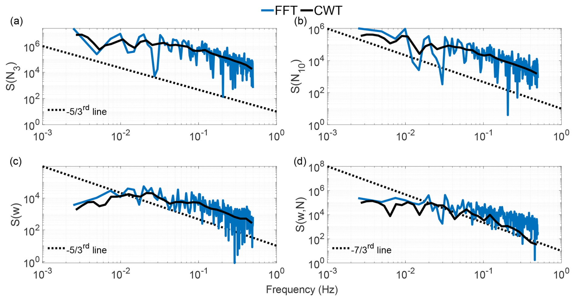
Figure 1 Power spectral density for (a) N₃, (b) N₁₀, (c) vertical wind velocity, and (d) 3–10 nm particle flux.

Figure 1 also shows some differences between FFT and CWT flux calculations, especially for fluxes at high frequencies. These differences are attributable primarily to non-stationarity in the aircraft data, as the platform moves through different air masses, meteorological conditions, and altitudes. FFT assumes stationarity over the entire analysis window and can therefore introduce artifacts under such conditions, whereas CWT provides time-localized frequency information that is more robust for non-stationary signals (Schaller et al., 2017). Li et al. (2023) evaluated uncertainties of turbulent flux calculation using both methods, finding that biases can range from 50 %–100 % of the spectrally complete flux. We note that the high-frequency deviations visible in the particle concentration spectra are not a consequence of FFT limitations but reflect the band-limited response of the CPC, which attenuates concentration fluctuations at frequencies above ∼0.3 Hz, as discussed in Sect. 2.8. The CWT's more conservative high-frequency response may better represent the actual resolvable flux contributions (Misztal et al., 2014).

To assess whether the calculated fluxes adequately represent both low- and high-frequency turbulent contributions, we conducted ogive analysis using the approach described by Foken et al. (2006). Mobile measurement platforms necessitate modified considerations for flux averaging intervals. Standard 30 min averaging periods used in stationary tower observations are inappropriate for aircraft measurements. Considering the aircraft's ground speed, a 90 s sampling period covers an equivalent air mass to that sampled by a stationary sensor over 30 min at typical wind speeds of 5 m s⁻¹. To enable direct comparison between ogives computed using FFT and CWT methods, normalization was applied according to Sun et al. (2018):

$$\begin{array}{}\text{(12)}& \widehat{\text{Og}}\left(f\right)={\displaystyle \frac{\text{Og}\left(f\right)}{\text{sgn}\mathit{\{}max(\text{Og}\left(f\right))+min(\text{Og}\left(f\right)\left)\mathit{\right\}}max\left(\right|\text{Og}\left(k\right)\left|\right)}}\end{array}$$

where sgn{x} represents the signum function, returning +1 for positive x, −1 for negative x, and zero when x equals zero. When the normalized ogive equals 1, the ogive value corresponds precisely to the covariance value for that averaging period. The advantage of this normalization approach is that it facilitates the identification of cases where low-frequency turbulence has an opposite sign to high-frequency turbulence. In such situations, large and small eddies transport material in opposing directions, indicating complex atmospheric processes such as counter-gradient transport. The normalized ogive plot visually reveals these opposing contributions through characteristic rise-and-fall patterns that might otherwise be obscured in non-normalized data.

Figure 2 illustrates the ogive as a function of distance covered by the aircraft for the same flight leg shown in Fig. 1. Signal frequency was converted to distance by dividing the aircraft speed (assumed to be constant at 100 m s⁻¹) by the frequency obtained from the FFT or CWT analysis. This plot reveals that the particle flux for this flight leg can be resolved by averaging over 40 km. While both FFT and CWT ogives show agreement for this case, such consistency cannot be expected universally; therefore, CWT fluxes are used throughout this study for the reasons discussed in previous sections.

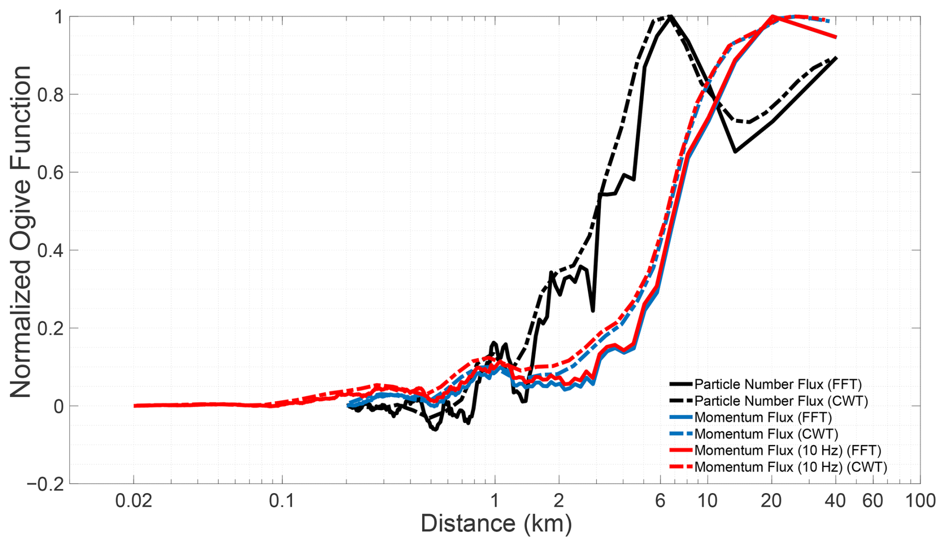
Figure 2 Normalized ogive function as a function of distance covered by the aircraft. The ogive represents the cumulative fractional contribution to total flux from high to low frequencies.

2.8 Flux loss correction

If the sensor used to measure fluxes are too slow to accurately capture the smaller eddies that contribute to the total flux, the turbulent fluxes will require correction. For micrometeorological flux measurements on towers at 10 m above the surface, instruments are typically operated at 10 Hz (Nyquist frequency = 5 Hz). Under typical wind speeds of 5 m s⁻¹, this sampling rate can resolve eddies as small as ∼1 m, ensuring that most energy-containing and inertial subrange eddies are captured (Aubinet et al., 2012; Lee et al., 2005; Stull, 1988).

However, airborne flux measurements present different challenges. The integral length scales of turbulent eddies increase approximately linearly with height within the surface layer (roughly the bottom 10 % of the boundary layer), then remain approximately constant above this level, limited by the boundary layer height (Kaimal and Finnigan, 1994). In the mixed layer portion of a typical boundary layer (above ∼100 m surface layer), integral length scales are typically 100–200 m (Lenschow and Stankov, 1986). At an aircraft ground speed of 100 m s⁻¹, the 1 Hz sampling provides 200 m spatial resolution, which approaches but does not fully resolve the integral length scale. Consequently, the sampling resolution approaches the lower limit for adequately resolving the dominant flux-carrying scales and may under sample contributions from smaller turbulent structures.

To address this limitation, we applied the approximations from Horst (1997) to estimate the ratio of measured flux (F_m) to spectrally complete flux (F) for different atmospheric stability conditions encountered during campaign flights:

$$\begin{array}{}\text{(13)}& {\displaystyle \frac{F_{\mathrm{m}}}{F}}={\displaystyle \frac{\mathrm{1}}{\mathrm{1}+(\mathrm{2}\mathit{\pi }{n}_{\mathrm{m}}{\mathit{\tau }}_{\mathrm{c}}\frac{\stackrel{\mathrm{‾}}{u}}{z}{)}^{\mathit{\alpha }}}}\end{array}$$

where F_m is the measured flux, F is the spectrally completeflux, $\stackrel{\mathrm{‾}}{u}$ is the magnitude of average wind speed, z is the height of the airplane, τ_c is the response time constant of the CPC, which was taken as 3.0 s, α = seven-eights and n_m=0.085 for neutral and unstable conditions (Pryor et al., 2007). Equation (13) was originally developed by Horst (1997) to estimate the attenuation of scalar flux measurements within the surface layer, but has been applied to aircraft measurements (Gioli et al., 2004), with corrected airborne fluxes showing good agreement with tower data when aircraft measurements were conducted over homogeneous surfaces at altitudes comparable to tower height.

To illustrate the practical importance of this correction, the $\frac{F_{\mathrm{m}}}{F}$ ratio varies substantially depending on measurement height and atmospheric stability conditions encountered during the campaign. For measurements conducted near the top of the marine boundary layer (∼1200–1400 m) under near-neutral to unstable conditions, $\frac{F_{\mathrm{m}}}{F}$ values approach unity (0.93–0.99), indicating that flux losses are modest at these heights where the dominant flux-carrying eddies are large relative to the CPC response limitation. However, for measurements conducted closer to the surface (∼30–550 m), $\frac{F_{\mathrm{m}}}{F}$ values range from 0.70 to 0.95, implying that uncorrected fluxes could underestimate the spectrally complete flux by up to 30 %. This highlights the importance of applying the flux loss correction, particularly for low-altitude flight legs where eddy sizes are smaller and the CPC response time constant becomes a more significant fraction of the dominant flux-carrying eddy turnover times.

Following the approach of Islam et al. (2022), we assessed the random uncertainty in particle flux due to counting statistics. We found it to be 2–3 orders of magnitude lower compared to the measured flux magnitudes reported in this study. Therefore, the correction due to discrete counting statistics of CPCs was not applied to this study.

Table 1 Summary of N₃₋₁₀ particle vertical turbulent flux estimates from aircraft campaigns with detection limits and flux loss assessment.

3 Results

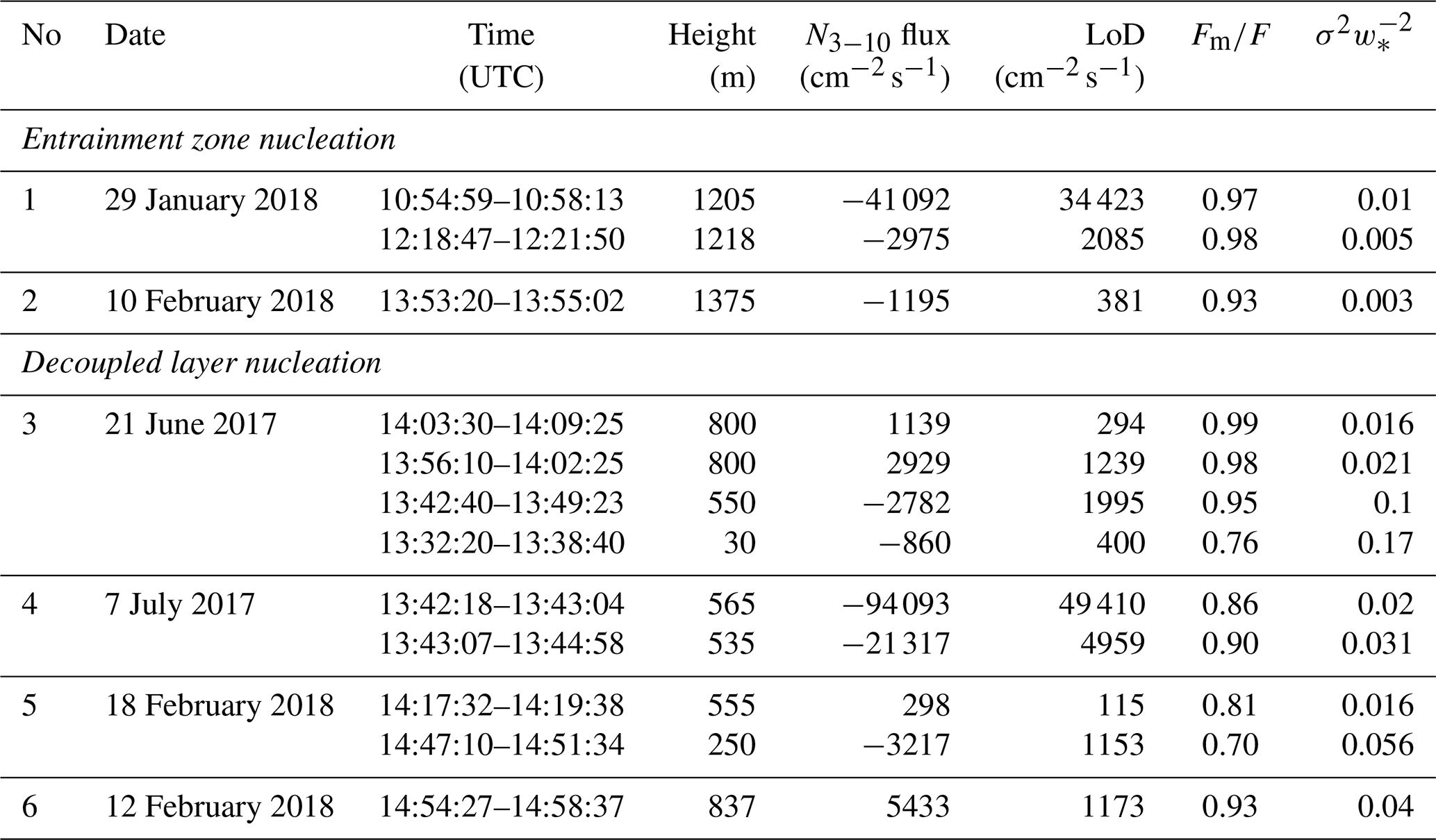
We examine two flight days as case studies of SPEs observed at varying altitudes above the ocean. Additional supporting flights are presented in the Supplement. Table 1 summarizes the N₃₋₁₀ vertical turbulent flux estimates derived from all six flight days analyzed in this study, grouped by the inferred nucleation regime. Flights 1 and 2 (29 January and 10 February 2018) are classified as entrainment zone nucleation events, where SPEs were detected near the top of the MBL at heights exceeding 1200 m. Flights 3–6 (21 June and 7 July 2017; 18 and 12 February 2018) are classified as decoupled layer nucleation events, with SPEs observed across a broader range of altitudes (30–837 m). For all events, the ratio of measured flux to the spectrally complete flux $\left(\frac{F_{\mathrm{m}}}{F}\right)$ exceeds 0.76, indicating minimal flux loss due to sensor response limitations. The normalized vertical velocity variance (${\mathit{\sigma }}_w^{\mathrm{2}}{w}_{\ast }^{-\mathrm{2}}$) is generally low, consistent with relatively quiescent turbulent conditions during the measurement periods. Negative flux values indicate downward transport of freshly nucleated particles from the entrainment zone toward the surface, while positive values suggest upward transport from a source within the decoupled sub-cloud layer. Two of these flight days, 29 January 2018 (Case 1) and 21 June 2017 (Case 2), are examined in detail as case studies in the following sections, with the remaining four flights presented as supporting examples in the Supplement.

3.1 Case 1: SPE occurring in the entrainment zone near the top of the marine boundary layer

Figures 3–5 present data collected on 29 January 2018 with an additional example from 10 February 2018, shown in Figs. S9–S11. Back-trajectory analysis (not shown) indicates that the sampled airmasses had been circulating around the Azores for the preceding three days and were therefore likely less polluted than North American outflow air masses. Figure 3 shows a multi-panel time series covering approximately 3.5 h of flight operations. The aircraft initially ascended to ∼2500 m but generally remained below ∼1500 m for most of the flight (Fig. 3a). The flight trajectory (Fig. 3b) reflects predominantly east–west movement across the Azores region, spanning latitudes from approximately 38.7 to 39.4° N and longitudes from −28.4 to −27.4° W. Drizzle number concentration measured by 2DS (purple and blue lines in Fig. 3b) was absent or low during the selected SPE periods. Elevated drizzle number concentration, together with high liquid water content regions (orange in Fig. 3d), mark frequent cloud encounters. Following our quality control procedures, all N₃₋₁₀ concentration data with LWC $\ge \mathrm{3}\times {\mathrm{10}}^{-\mathrm{3}}$ g m⁻³ were excluded from analysis to avoid contamination from cloud droplet shattering artifacts. Pink-shaded periods mark the intervals chosen for detailed analysis, which exhibited simultaneous increases in both N₃ and N₁₀ concentrations exceeding 10⁴ cm⁻³ (indicating an SPE). Supermicron particle concentration (blue in Fig. 3c) as well as total particle surface area (green in Fig. 3c) were also low during the selected SPE periods, indicating the absence of particles such as sea spray aerosols.

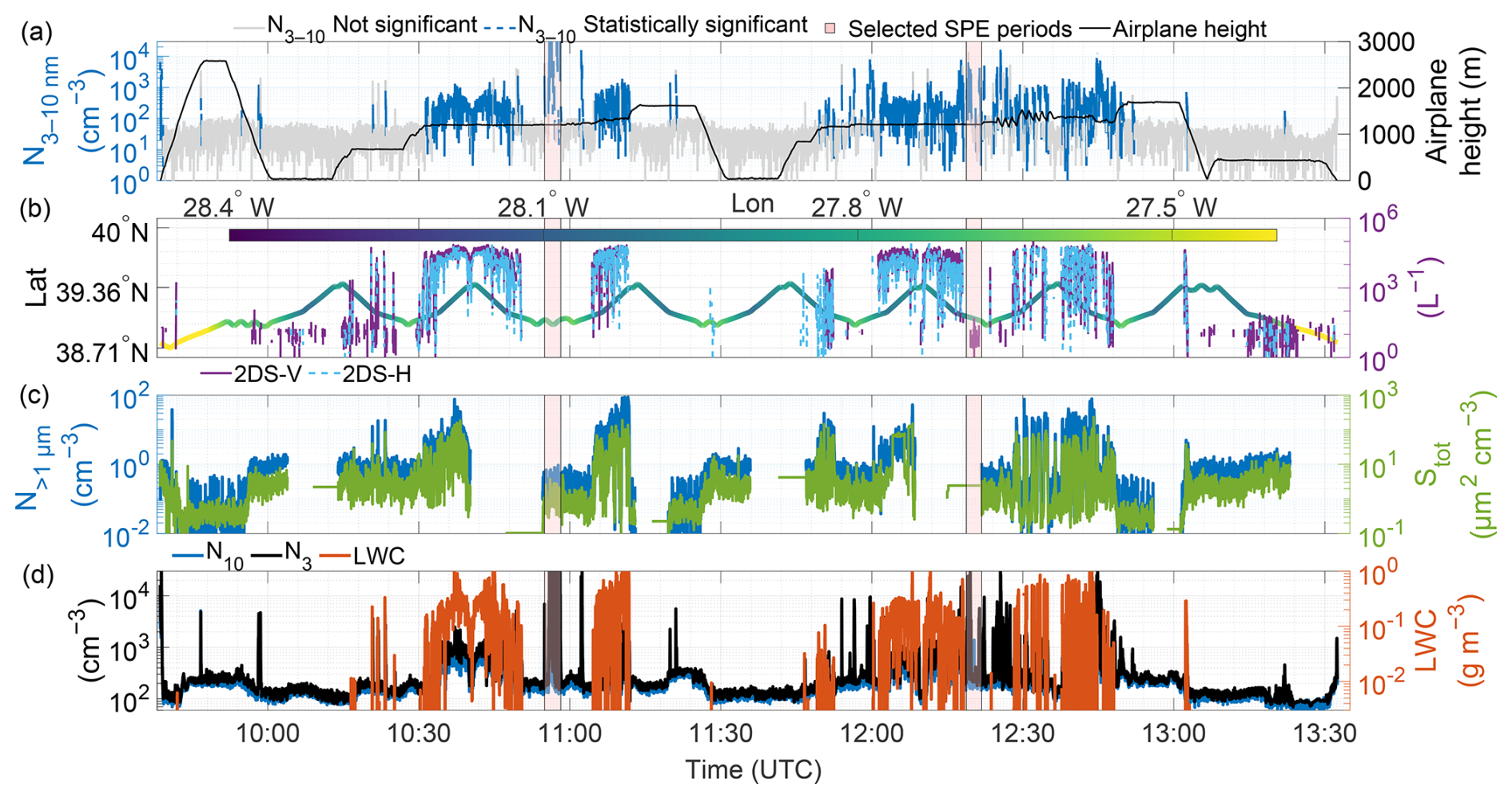
Figure 3 Multi-parameter time series from the 29 January 2018 flight. (a) N₃₋₁₀ particle concentrations and aircraft altitude; (b) aircraft position (latitude and longitude) and drizzle number concentration; (c) supermicron particle concentration and total particle surface area (S_tot); (d) particle number concentrations (N₁₀ and N₃) and liquid water content. Gaps in the time series indicate the missing data.

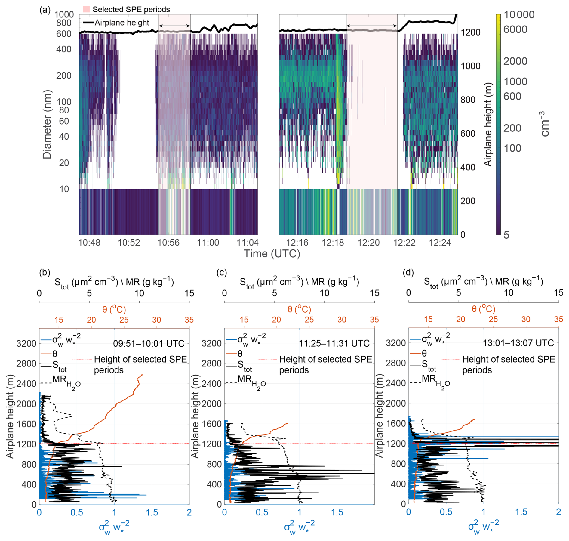
Figure 4 (a) Size-resolved particle number concentrations (10–600 nm) from FIMS as a function of time and altitude, with N₃₋₁₀ concentrations shown in the lower strip. Pink shading indicates selected SPE periods. (b–d) Vertical profiles of potential temperature (θ), normalized vertical velocity variance (${\mathit{\sigma }}_w^{\mathrm{2}}{w}_{\ast }^{-\mathrm{2}}$), total particle surface area (S_tot), and water vapor mixing ratio (MR${}_{{\mathrm{H}}_{\mathrm{2}}\mathrm{O}}$) for three time periods nearest to the selected SPE periods: (b) 09:51–10:01 UTC, (c) 11:25–11:31 UTC, and (d) 13:01–13:07 UTC. Gaps in the time series indicate the missing data.

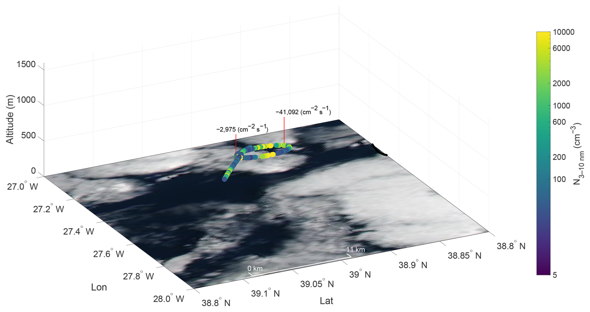
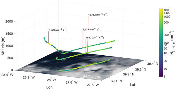
Figure 5 Spatial distribution of N₃₋₁₀ particle concentrations along the flight track at ∼1200 m altitude during the period highlighted in Figs. 3 and 4. Calculated vertical turbulent fluxes are labeled at their respective measurement locations. Color scale indicates N₃₋₁₀ particle number concentrations (cm⁻³). The background shows a true-color satellite-corrected reflectance image from the overpass at 15:15 UTC, with the ocean surface appearing dark and clouds appearing white. Credit: NASA Worldview Snapshots.

Figure 4a shows the temporal evolution of particle concentration between $\sim \mathrm{10}:\mathrm{47}$–11:05 and $\sim \mathrm{12}:\mathrm{15}$–12:25 UTC. The colormap represents FIMS-derived, size-resolved aerosol number concentrations (10–600 nm diameter), varying across time and altitude, while the lower panel displays N₃₋₁₀ concentrations. The two pink-highlighted intervals are the same as in Fig. 3. The high particle concentration spike observed $\sim \mathrm{12}:\mathrm{18}$ UTC coincides with elevated LWC and drizzle concentration (Fig. 3d) and was excluded from analysis following our quality control procedures (Sect. 2.3.1). Weber et al. (1998) documented that cloud droplet shattering can produce artifactual particle concentrations as small as 3 nm in airborne CPC measurements, making this the most plausible explanation for the observed spike. Aircraft exhaust contamination can be ruled out, as the nearest prior flight transect over this region occurred approximately half an hour earlier at an altitude ∼60 m lower, more than sufficient time and vertical separation for complete plume dispersal. This data point was therefore excluded from all flux calculations as the concurrent LWC exceeded the quality control threshold of $\mathrm{3}\times {\mathrm{10}}^{-\mathrm{3}}$ g m⁻³.

Figure 4b–d present vertical profiles of potential temperature, normalized vertical velocity variance (${\mathit{\sigma }}_w^{\mathrm{2}}{w}_{\ast }^{-\mathrm{2}}$) i.e., (the vertical velocity variance normalized by the square of the convective velocity scale), total particle surface area, and the water vapor mixing ratio at three locations nearest to the pink-highlighted intervals. Sharp gradients in the potential temperature (orange) mark the top of the MBL, defining the capping inversion that suppresses vertical mixing between the boundary layer and the free troposphere. The co-occurrence of these temperature gradients with elevated normalized vertical velocity variance (${\mathit{\sigma }}_w^{\mathrm{2}}{w}_{\ast }^{-\mathrm{2}}$) near the inversion level indicates the presence of an entrainment zone, where thermodynamic forcing (including cloud-top radiative cooling and wind shear) drives mixing between the free tropospheric air above and the convective boundary layer below (Boers and Eloranta, 1986). Figure 4b–d reveal a deep boundary layer with the entrainment zone between approximately 1200–1400 m, consistent with previous estimates that entrainment zones typically comprise 20 %–40 % of boundary layer depth (Martin et al., 2014).

Figure 4b–d present the profiles of (${\mathit{\sigma }}_w^{\mathrm{2}}{w}_{\ast }^{-\mathrm{2}}$), a metric that characterizes the intensity of turbulent structures in convective boundary layers (Deardorff, 1974; Dewani et al., 2023). These profiles show elevated (${\mathit{\sigma }}_w^{\mathrm{2}}{w}_{\ast }^{-\mathrm{2}}$) values near the ocean surface and within the entrainment zone, with minimal values in the free troposphere, where significant turbulence is absent.

The water vapor mixing ratio profiles in Fig. 4b–d reveal evolving boundary layer moisture structure during the flight. The early profile (Fig. 4b) shows a relatively well-mixed moisture distribution below the capping inversion at ∼1200 m, with a sharp decrease into the drier free troposphere above. The latter profiles (Fig. 4c and d) exhibit a two-step moisture structure, with a sharper gradient near ∼600 m suggesting progressive decoupling of the boundary layer during the course of the flight, separating a moister surface layer from a drier sub-cloud layer above. Despite some vertical variability shown in Fig. 4b–d, the total particle surface area (S_tot) remained relatively low throughout the flight, falling well below the campaign averages of ∼30 µm² cm⁻³ in the surface mixed layer and ∼10 µm² cm⁻³ in the upper decoupled layer reported by Zheng et al. (2021). Figure 4c also shows a distinct S_tot maximum at an altitude where small gradients in both potential temperature and mixing ratio suggest the presence of an entrainment layer. The pronounced S_tot increase could indicate a nucleation occurring at this location (see Case 2 below), although this hypothesis could not be independently verified looking at the N₃₋₁₀ data in this case. Figure 4c shows that the entrainment zone and free troposphere were characterized with extremely low S_tot values.

Figure 5 presents the spatial distribution of N₃₋₁₀ particle concentrations along the flight path at ∼1200 m altitude (dashed lines in Fig. 4b–d), with the calculated vertical turbulent fluxes labeled at their respective measurement locations. Concentrations up to 10 000 cm⁻³ were observed along the flight track, with the highest values concentrated within a horizontal extent of less than 10 km. The substantial downward fluxes of N₃₋₁₀ particles (−41 092 and −2975 ${\mathrm{cm}}^{-\mathrm{2}}{\mathrm{s}}^{-\mathrm{1}}$) at ∼1200 m both exceed their respective limits of detection (Table 1), confirming that the observed downward transport represents a statistically significant atmospheric signal rather than measurement noise. The downward flux direction indicates that the source of freshly nucleated particles was located above the measurement altitude, within the entrainment zone, while the large difference in flux magnitudes between the two events likely reflects spatial heterogeneity in source strength and the proximity of the aircraft to the nucleation zone during each transect. This interpretation is supported by the near-absence of N₃₋₁₀ at ∼1600 m during 11:14–11:25 and 12:51–13:01 UTC (Fig. 3), with the exception of brief concentration spikes of uncertain origin retained in the record due to insufficient evidence for their removal. The small particle size (3–10 nm) and limited horizontal extent of less than 10 km further argue against a free tropospheric nucleation source, as particles originating in the free troposphere would be expected to have grown substantially and the plume to have diluted during descent to measurement altitude. Several mechanisms could promote nucleation specifically within the entrainment zone, adiabatic cooling in the rising convective plumes, turbulent fluctuation in temperature and vapor concentration generated by entrainment, and dilution of mixed-layer air by the entrained free tropospheric air, causing a sudden reduction in preexisting aerosol surface area (Nilsson et al., 2001). The extremely low S_tot values observed in the entrainment zone and free troposphere (Fig. 4), falling well below the campaign averages, are consistent with this interpretation. These conditions are analogous to those identified in previous studies linking entrainment zone nucleation to reduced condensation sink environments (Größ et al., 2018; Meskhidze et al., 2019; Nilsson et al., 2001). Figures S10 and S11 provide additional support, showing a downward flux of N₃₋₁₀ particles (−1195 ${\mathrm{cm}}^{-\mathrm{2}}{\mathrm{s}}^{-\mathrm{1}}$) at 1375 m with complete absence of N₃₋₁₀ above ∼1400 m, consistent with SPE occurrence specifically within the entrainment zone between 1375–1400 m.

Figures 3–5 and the flux analysis (Table 1) demonstrate that the entrainment zone nucleation near the MBL top occurred on two days (29 January and 10 February 2018), representing nearly 5 % of flight days. Despite a relatively small horizontal extent (<10 km), these newly formed particles can be entrained in the boundary layer via vertical turbulent processes, potentially playing an important role in marine aerosol number budget and, given sufficient time for growth to CCN-relevant sizes, potentially influencing cloud condensation nuclei concentrations for marine stratocumulus clouds.

3.2 Case 2: SPE occurring at the interface between the well-mixed surface layer and the decoupled layer

Figures 6–8 present data from 21 June 2017, with additional examples from 7 July 2017, 18 February 2018 and 12 February 2018, shown in Figs. S12–S14, S15–S17, and S18–S20. Back-trajectory analysis (not shown) indicates that the sampled airmasses originated from the Arctic and were therefore expected to be relatively clean. Figure 6 covers approximately 4 h of flight operations, during which the aircraft initially flew at very low altitudes (∼30 and 50 m) near 12:00 and 13:30 UTC before gradually ascending to ∼1000 m. Drizzle number concentration by 2DS (purple and blue lines in Fig. 6b) was absent or below the threshold during the selected SPE periods. Multiple events with N₃₋₁₀ concentrations from 10² to 10⁴ cm⁻³ were observed throughout the second half of the flight. The flight trajectory (Fig. 6b) reflects predominantly east-west movement, spanning latitudes from approximately 38.6 to 39.3° N and longitudes from −28.4 to −27.4° W. Pink-highlighted intervals show periods with concurrent increases in N₃ and N₁₀ concentrations exceeding 10³ cm⁻³, indicating occurrences of SPEs. As in Case 1, supermicron particle concentrations (blue in Fig. 6c) and total particle surface area (green in Fig. 6c) remained low during the selected SPE periods, indicating the absence of coarse-mode particles such as sea spray.

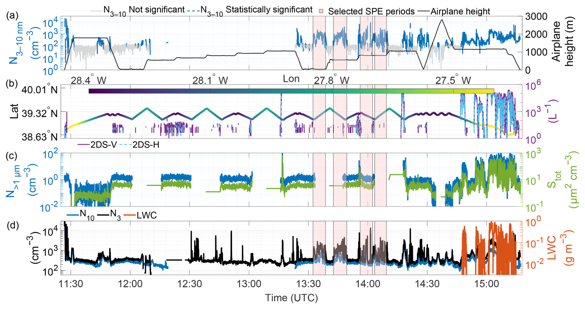
Figure 6 Same as Fig. 3 but for 21 June 2017. Gaps in the time series indicate the missing data.

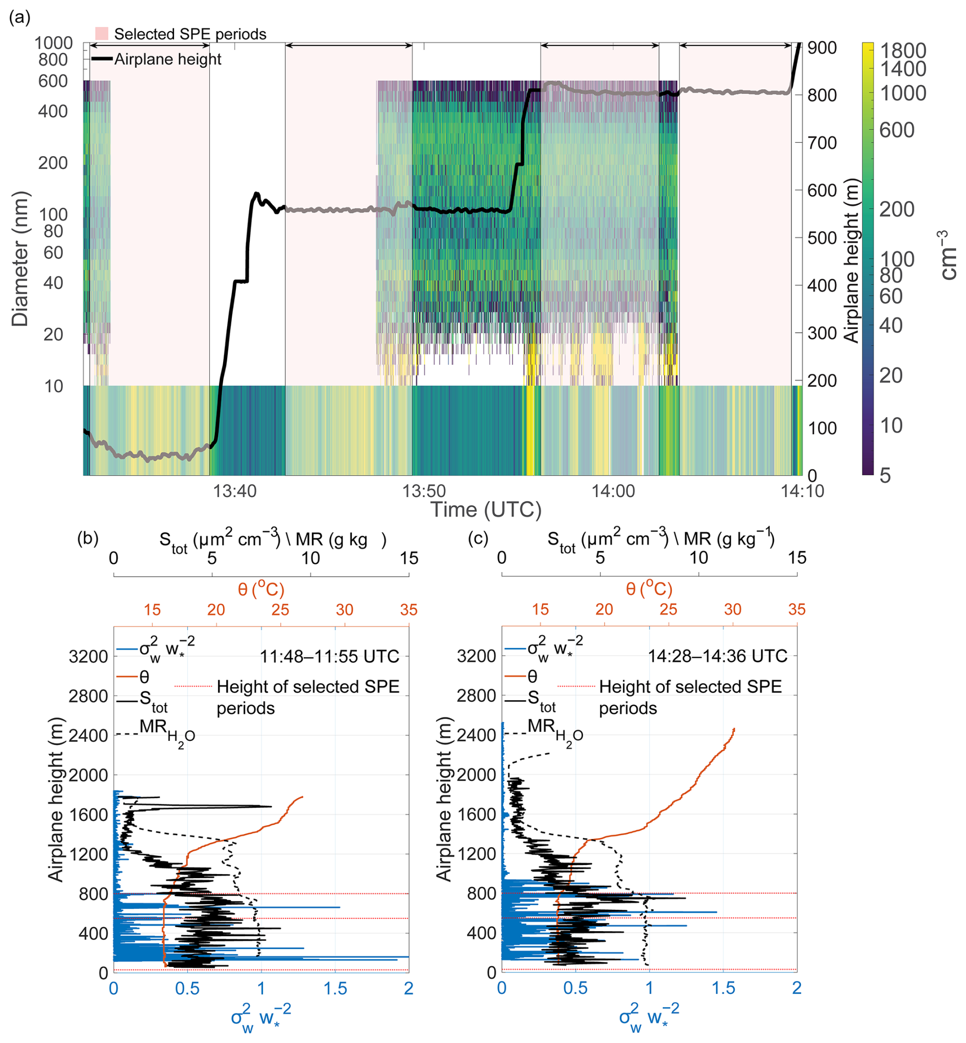
Figure 7 Same as Fig. 4, but for 21 June 2017. Gaps in the time series indicate the missing data.

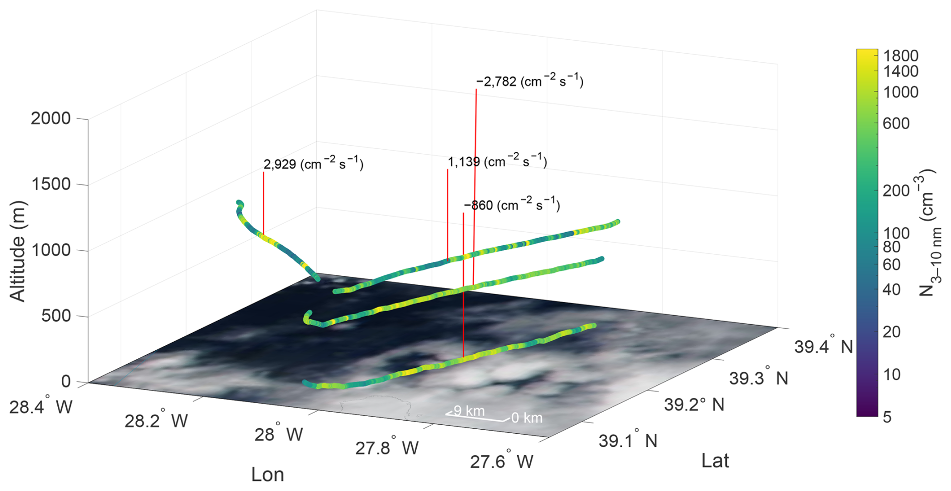
Figure 8 Spatial distribution of N₃₋₁₀ particle concentrations along the flight track at varying altitudes (30, 550, and 800 m) during the period highlighted in Figs. 6 and 7. Calculated vertical turbulent fluxes are labeled at their respective measurement locations. Color scale indicates N₃₋₁₀ particle number concentrations (cm⁻³). The background shows a true-color satellite reflectance image from the overpass at 14:15 UTC, with the ocean surface appearing dark and clouds appearing white. Credit: NASA Worldview Snapshots.

Figure 7a shows size-resolved particle number concentration evolution during 13:30–14:20 UTC, encompassing the four pink-highlighted intervals from Fig. 6. The lower panel Fig. 7a displays N₃₋₁₀ particle concentrations. High N₃₋₁₀ concentrations were encountered at multiple altitudes, with maximum values exceeding 1800 cm⁻³ at ∼800 m.

The potential temperature and water vapor profiles (Fig. 7b and c) show the MBL structure consisting of a well mixed surface layer extending to ∼700 m and a decoupled upper boundary layer between ∼700–1300 m. Decoupled structures typically form from radiative heating of the cloud layer and evaporative cooling in the sub-cloud layer, which stabilize the boundary layer and suppress vertical mixing (Galewsky et al., 2022; Jones et al., 2011; Wood and Bretherton, 2004). Sharp gradients in both potential temperature and mixing ratio around 1300 m marking the entrainment zone, above which the free troposphere begins above 1400 m. The (${\mathit{\sigma }}_w^{\mathrm{2}}{w}_{\ast }^{-\mathrm{2}}$) profiles show higher magnitudes in the mixed layer (indicating active turbulence) and low magnitudes in both the decoupled layer (due to stratification and suppressed vertical mixing) and free troposphere. Total particle surface area remained low in the mixed layer but increased considerably toward the top of the mixed layer before decreasing in the decoupled layer and reaching very low values in the free troposphere.

Figure 8 shows N₃₋₁₀ particle concentrations along flight paths at varying altitudes: 30 m, 550 m, and two segments at 800 m. We separated the 800 m path to prevent the airplane sampling the same airmass because from 13:55–14:03 UTC the aircraft flew along the prevailing wind direction, then changed direction by 90° to fly perpendicular to the wind. The positive vertical turbulent fluxes at 800 m and negative values below suggest the SPE occurred between 550–800 m, likely at the top of the well mixed layer or the bottom of the decoupled layer.

The nucleation processes in the entrainment zone and at the base of the decoupled layer could be mechanistically similar. Both locations feature the convergence of distinct air masses, in this case, the well-mixed surface layer and the stratified decoupled layer above, which generates turbulent mixing and aerosol dilution effects. While less pronounced than at the boundary layer top, the interface between these layers exhibits comparable thermodynamic conditions: potential temperature gradients, contrasting vapor concentrations, and localized adiabatic cooling. Figure 7 demonstrates that the decoupled layer maintains significantly lower aerosol surface area concentrations relative to the well-mixed layer below, establishing conducive conditions for nucleation when air mass mixing occurs. A key distinction, however, lies in the spatial characteristics, whereas entrainment zone nucleation showed limited horizontal extent (<10 km), the decoupled layer event spanned at least 50–60 km, suggesting either more persistent favorable conditions or a fundamentally different source mechanism operating over regional scales.

Figure 8 reveals a strong negative flux of N₃₋₁₀ (−2782 ${\mathrm{cm}}^{-\mathrm{2}}{\mathrm{s}}^{-\mathrm{1}}$) at 550 m that is nearly three times greater in magnitude than the flux at 30 m (−860 ${\mathrm{cm}}^{-\mathrm{2}}{\mathrm{s}}^{-\mathrm{1}}$), likely due to particle evolution through growth and coagulation, and dilution processes during vertical transport. The positive fluxes of N₃₋₁₀ observed at 800 m (2929 and 1139 ${\mathrm{cm}}^{-\mathrm{2}}{\mathrm{s}}^{-\mathrm{1}}$) suggest that nucleation initiated either at the top of the well-mixed boundary layer or at the bottom of the overlying decoupled layer. This bidirectional flux structure suggests that newly formed particles were transported both upward and downward from the formation zone through turbulent mixing. The comprehensive analysis presented in Figs. 6–8, combined with the flux calculations in Table 1, provides some evidence that SPEs can originate within decoupled layer structures, constituting a significant source of secondary marine aerosols in stratified boundary layer conditions.

4 Discussion

This study demonstrates the value of vertical turbulent flux measurements for characterizing small particle events (SPE) in remote marine boundary layers. By deriving 3–10 nm particle fluxes from aircraft measurements during the ACE-ENA campaign, we identified two mechanistically distinct SPE scenarios that challenge conventional understanding of marine aerosol sources. Critically, while flux sign alone identifies the vertical location of the particle source, flux magnitude serves two additional essential roles: first, it must exceed the limit of detection to confirm that the observed directional transport represents a statistically significant atmospheric signal rather than measurement noise; and second, it provides quantitative constraints on source strength that cannot be obtained from sign alone.

Our analysis reveals different SPE mechanisms operating in the marine boundary layer. The first mode – entrainment zone nucleation – occurs at the boundary layer top (1200–1400 m) where several factors create favorable conditions: (1) dilution of mixed-layer air by entrained free tropospheric air causes sudden decreases in preexisting aerosol surface area, (2) adiabatic cooling in rising convective plumes reduces saturation vapor pressures, and (3) turbulent fluctuations in temperature and vapor concentration enhance nucleation rates (Größ et al., 2018; Nilsson et al., 2001). Strong downward fluxes (up to −41 092 ${\mathrm{cm}}^{-\mathrm{2}}{\mathrm{s}}^{-\mathrm{1}}$) exceeding the limit of detection confirm that nucleation occurs specifically within this ∼200 m entrainment layer, while the absence of 3–10 nm particles above the entrainment zone rules out a free tropospheric source. The limited horizontal extent (2–9 km) of these events is consistent with the spatial scales of organized convective structures that develop in the upper decoupled marine boundary layer following cold front passages in the Azores region, where cumulus-associated drizzle reduces the condensation sink to levels favorable for nucleation (Etling and Brown, 1993; Zheng et al., 2021).

The large difference in flux magnitudes between the two entrainment zone events (−41 092 vs. −2975 ${\mathrm{cm}}^{-\mathrm{2}}{\mathrm{s}}^{-\mathrm{1}}$) provides information that flux sign alone cannot supply: it reflects spatial heterogeneity in source strength and the proximity of the aircraft to the nucleation zone during each transect. As turbulent intensity is unlikely to have changed substantially over the ∼1–2 h interval separating the two transects, the order-of-magnitude difference in flux magnitude more plausibly reflects variation in the horizontal distance between the aircraft and the nucleation zone, or spatial heterogeneity in source strength, rather than a change in the turbulent transport efficiency itself. These flux magnitudes, integrated over the duration of the events, represent a substantial source of freshly nucleated particles to the marine aerosol number budget, constraints that can be used directly to evaluate nucleation parameterizations in regional and global models. While the ultimate contribution of these particles to CCN populations depends on growth timescales and loss processes during vertical transport (requiring ∼24–48 h at typical marine growth rates of ∼1 nm h⁻¹ to reach CCN-relevant sizes; Zheng et al., 2021), the flux-based constraints provided here represent a necessary observational foundation for quantifying this contribution in future studies. Our analysis reveals a second distinct mode of SPE occurring within decoupled marine boundary layer structures, where particles originate at the interface between the well-mixed surface layer and the overlying decoupled layer (∼700–800 m altitude). Unlike entrainment zone nucleation, which occurs at the boundary layer top, decoupled layer nucleation operates within the interior of the boundary layer at the interface between the well-mixed surface layer and the overlying stratified layer. Both mechanisms share key preconditions: convergence of air masses with contrasting thermodynamic properties, gradients in potential temperature and water vapor mixing ratio, and aerosol dilution that suppresses the condensation sink. However, the decoupled layer mode is distinguished by stratified vertical mixing that confines turbulent exchange to a narrower altitude range. It is also characterized by a substantially larger horizontal extent (>50 km) compared to entrainment zone events (<10 km), suggesting either more persistent favorable conditions or a fundamentally different source mechanism operating at regional scales. The substantial negative flux magnitudes observed at intermediate altitudes (−2782 ${\mathrm{cm}}^{-\mathrm{2}}{\mathrm{s}}^{-\mathrm{1}}$ at 550 m) combined with positive fluxes aloft demonstrate active particle redistribution throughout the marine boundary layer. The factor of ∼3 difference in flux magnitude between the 550 m and 30 m levels (−2782 vs. −860 ${\mathrm{cm}}^{-\mathrm{2}}{\mathrm{s}}^{-\mathrm{1}}$) is consistent with attenuation of the particle flux during downward transport through dilution with ambient air, as well as losses through coagulation and growth out of the 3–10 nm size range. This vertical divergence in flux magnitude represents a quantitative signature of particle evolution during transport that flux sign alone would be incapable of revealing. This mode represents a significant and previously underappreciated source of secondary marine aerosols that can efficiently contribute to regional aerosol budgets through direct incorporation into the surface mixed layer where particles undergo growth to cloud-relevant sizes.

5 Conclusions

The occurrence of newly formed particles in marine environments has been documented in a number of previous studies. Wiedensohler et al. (1996) observed sub-20 nm particles originating from the free troposphere or cloud tops within the MBL and mixed downwards over the open ocean, suggesting in-situ production based on correlations with absolute humidity. Covert et al. (1992) reported sub-20 nm particle production near precipitating cloud tops within the MBL, where larger particles acting as condensation sinks had been scavenged by precipitation, with sub-20 nm particles dominating 10 % of the campaign and indicating episodic rather than continuous production. O'Dowd et al. (2002) documented NPF events at the coastal Mace Head station when marine air masses encountered biogenic emissions from the intertidal zone. The ACORES campaign, conducted over the Azores at the same time as ACE-ENA, reported freshly nucleated particle bursts near the cloud top exceeding background MBL concentrations by more than an order of magnitude (Siebert et al., 2021). Concurrent helicopter-borne particle flux measurements over the Azores during ACORES (Lückerath et al., 2022) also documented particle fluxes in the marine boundary layer, providing complementary observational context to our aircraft-based approach. The prevailing theoretical framework, based on relatively high sea spray aerosol surface area acting as condensation and coagulation sinks (Bates et al., 1998; Pirjola et al., 2000), nonetheless predicted that NPF should rarely occur in remote marine boundary layers over open oceans. Our flux-based observations build on this existing framework by providing the first direct constraints on the vertical source location and strength of freshly nucleated particles in the remote marine boundary layer. Low aerosol surface area and specific meteorological configurations can create localized or regional zones where conditions become favorable. For entrainment zone and decoupled layer events, extremely low aerosol concentrations, combined with turbulent mixing and adiabatic cooling can create a transient “window” where nucleation can proceed despite moderate surface area concentrations lower in the boundary layer. Recent ground-based observations from the same campaign (Zheng et al., 2021) documented frequent NPF events but could not definitively determine vertical location. Our flux-based approach resolves this ambiguity by providing direct evidence of where particles originate relative to the measurement location. The negative (downward) fluxes in Case 1 unambiguously demonstrate an above-aircraft source, while the bidirectional fluxes in Case 2 indicate a distributed source encompassing the measurement altitude.

These findings have important implications for understanding marine aerosol budgets. The spatial scales of these two SPE modes differ by an order of magnitude: entrainment zone events exhibited limited horizontal extents (<10 km), consistent with localized convective structures, while decoupled layer events spanned regional scales (50–60 km), suggesting fundamentally different formation mechanisms or persistence of favorable conditions. For the entrainment zone mode, while the aircraft sampled the SPE for only ∼4 min during each transect due to its high ground speed, NPF events in marine and continental environments are typically observed to persist for 2–5 h (Islam et al., 2022; Kulmala et al., 2004; Zheng et al., 2021). Assuming the measured downward flux of −41 092 ${\mathrm{cm}}^{-\mathrm{2}}{\mathrm{s}}^{-\mathrm{1}}$ is representative of a nucleation event of typical duration of ∼3 h and using a mixed layer depth of ∼1200 m, the estimated increase in vertically integrated particle number concentration is approximately:

$$\begin{array}{}\text{(14)}& \mathrm{\Delta }{N}_{\mathrm{3}-\mathrm{10}}\approx \left|F\right|\times {\displaystyle \frac{\mathrm{\Delta }t}{z_{\text{MBL}}}}={\displaystyle \frac{\mathrm{41}\mathrm{092}\times \mathrm{10}\mathrm{800}}{\mathrm{1.2}\times {\mathrm{10}}^{\mathrm{5}}}}\approx \mathrm{3700}{\mathrm{cm}}^{-\mathrm{3}}\end{array}$$

where F is the flux in ${\mathrm{cm}}^{-\mathrm{2}}{\mathrm{s}}^{-\mathrm{1}}$, Δt is the event duration in seconds, and z_MBL is the mixed layer depth in cm. This represents a substantial addition to the total particle number concentration in the surface mixed layer, noting that this estimate refers to freshly nucleated 3–10 nm particles rather than CCN-relevant particles. The fraction surviving to CCN-relevant sizes (>50–80 nm) depends on growth rates and loss processes that cannot be quantified from single aircraft transects alone. However, Zheng et al. (2021) estimated that under favorable conditions at the same site, newly formed particles contributed on average ∼50 % of total CCN concentrations following cold front passages, suggesting that even accounting for coagulation losses, the contribution of entrainment zone nucleation to the marine CCN budget may be substantial. Entrainment zone nucleation, despite its limited horizontal extent, may contribute significantly to the marine aerosol number budget through sustained downward transport via convective mixing. Though flux magnitudes for the decoupled layer nucleation events (−2782 ${\mathrm{cm}}^{-\mathrm{2}}{\mathrm{s}}^{-\mathrm{1}}$) are less pronounced, their large spatial extent likely results in comparable or larger aggregate contributions to regional aerosol budgets. We note that the contribution of freshly nucleated particles to CCN population depends on growth rates and loss processes during transport and cannot be assessed from short-term measurements alone. The flux magnitudes and vertical source locations reported here provide the observational foundation needed to evaluate this contribution quantitatively in future studies combining particle flux measurements with growth rate and CCN closure analyses.

Our observations, combined with the longer history of marine NPF observations cited above and recent ground-based measurements from the same campaign (Zheng et al., 2021), suggest that the contribution of in-situ marine boundary layer nucleation to the aerosol budget may be more significant than current model representations assume. Climate models have historically followed theoretical expectations that marine boundary layer nucleation should be negligible, instead representing new particles as primarily originating from free tropospheric entrainment or long-range continental transport (Clarke et al., 2013; Logan et al., 2014), with marine boundary layer nucleation treated as negligible. The frequent occurrence of SPE during the ACE-ENA campaign (entrainment zone nucleation in 2 and decoupled layer nucleation in 4 of 39 flights analyzed) suggests that marine boundary layer nucleation – in both modes – may be more climatologically important than previously recognized. Given that marine boundary layer cloud microphysical properties exhibit the highest sensitivity to aerosol changes (Bellouin et al., 2020; Zhang et al., 2024), and that even modest changes in CCN concentrations can substantially affect cloud radiative forcing in these pristine environments, proper representation of NPF sources is critical for reducing uncertainties in aerosol-cloud interaction estimates.

The continuous wavelet transform (CWT) approach proved essential for deriving reliable fluxes from fast-moving aircraft platforms. Traditional eddy covariance methods require stationarity conditions that are difficult to maintain during aircraft sampling, where the platform continuously moves through different air masses. The CWT method's ability to handle non-stationary data while avoiding systematic errors from linear detrending (Rannik and Vesala, 1999; Schaller et al., 2017) enabled flux calculations even during complex meteorological conditions. Our detailed analysis of frequency response and flux loss corrections demonstrates that 1 Hz CPC measurements, while not ideal, can resolve sufficient turbulent scales to capture the dominant flux contributions when proper corrections are applied. Importantly, flux magnitudes (not just flux sign) provide essential scientific value: they must exceed the limit of detection to confirm statistical significance, they constrain source strength and proximity, and they provide quantitative inputs for evaluating nucleation parameterizations in regional and global models. As the scientific community works to reduce uncertainties in aerosol-cloud interactions, flux-based approaches offer a promising path forward for understanding how, where, and when new particles form in Earth's remote marine atmosphere.

Several limitations warrant acknowledgment. First, our 3–10 nm size range likely misses the initial nucleation at molecular cluster sizes (∼1–3 nm), meaning we observe “small particle events” rather than nucleation itself. However, the rapid appearance of 3–10 nm particles with clear vertical structure in turbulent fluxes provides strong indirect evidence for nearby nucleation. Second, the aircraft's high ground speed (∼100 m s⁻¹) compared to typical tower-based measurements introduces challenges for capturing the full turbulent spectrum, particularly at lower altitudes where eddy sizes are smaller. Our flux loss corrections ($F_{\mathrm{m}}/F$ ratios of 0.70–0.99) account for this limitation but introduce additional uncertainty. Third, we cannot determine definitively the exact horizontal extent of NPF events from single aircraft transects, though crosswind sampling provides minimum extent estimates.

Future directions

This work establishes aircraft-derived aerosol fluxes as a valuable tool for characterizing marine boundary layer aerosol sources. Several directions would advance understanding:

Slower aircrafts:

unmanned aerial vehicles operating at 30–40 m s⁻¹ would better resolve small-scale turbulence, particularly near the surface, where flux loss corrections are currently largest, improving flux accuracy and enabling more detailed vertical structure analysis.

Expanded measurements:

simultaneous flux measurements of precursor gases (H₂SO₄, NH₃, amines, organics) would directly test hypotheses about nucleation mechanisms and identify which chemical pathways dominate in different scenarios.

Multi-aircraft coordination:

coordinated measurements from more than one aircraft at different altitudes could directly observe vertical particle transport rates and evolution, constraining growth rates and loss processes during transit.

Longer-term statistics:

expanding beyond campaign-based measurements to seasonal or annual timescales would quantify the climatological importance of different NPF modes and their relationships to synoptic meteorological patterns.

Model evaluation:

using observed flux magnitudes and vertical source locations as benchmarks for evaluating marine boundary layer nucleation parameterizations in regional and global models would improve their representation of aerosol-cloud interactions and reduce uncertainties in aerosol indirect forcing estimates.