Near-threshold aeolian sand transport: effects of boundary layer flow conditions

Boundary layer thickness is a critical factor in aeolian sand transport, as it governs the scale of energy-containing turbulent structures, yet its specific mechanisms remain inadequately quantified. Previous studies have established the role of turbulence in particle entrainment but often overlook systematic variations in boundary layer thickness. This study aims to clarify how boundary layer thickness modulates wall-shear stress fluctuations, threshold wind velocities, sand flux, and particle kinematics. We use the three-dimensional large-eddy simulation coupled with a saltation model to investigate these interactions. Results reveal that increased boundary layer thickness enhances extreme-value probability density of wall-shear stress and significantly lowers impact entrainment and rebound thresholds – the latter dropping to less than 50 % of conventional wind-tunnel values. Sand transport response is velocity-dependent: at low velocities, transport rises markedly with thickness under fluid-driven entrainment; the effect diminishes at moderate velocities; and at high velocities, transport scales proportionally with thickness under splash-dominated entrainment. Moreover, thicker boundary layers intensify near-bed particle activity, elevating particle velocities and concentrations, reducing variability, increasing saltation height, and enlarging mean and variance of airborne particle diameters. These findings elucidate how boundary layer thickness modulates aeolian sand transport via turbulence–particle interactions, offering key insights for improving atmospheric and climate models and advancing the physics of turbulence-driven sediment transport in atmospheric boundary layer.

1 Introduction

Wind-driven soil particle movement, also known as aeolian transport, is a key geological and climatic process in arid and desert regions (Shao, 2008). Near-threshold aeolian sand transport occurs around the threshold wind velocity and is characterized by intermittent bursts of intense activity separated by quiescent periods (Stout and Zobeck, 1997; Leenders et al., 2005; Carneiro et al., 2015; Martin and Kok, 2018). Driven by natural wind, this highly unstable process significantly contributes to total mass flux and plays a crucial role in dune evolution, soil erosion, and dust emission. However, its quantitative prediction remains challenging (Martin and Kok, 2018) due to the multiscale nature of turbulent wind fluctuations (Butterfield, 1998; Mathis et al., 2009; Huang et al., 2020; Zhang et al., 2022) and the path-dependent response of sediment transport to these fluctuations (Kok, 2010a).

Accurate prediction of transport rate and intensity is essential for understanding the formation and evolution of aeolian landforms (Sherman et al., 1998). Modeling efforts have combined theoretical, experimental, and numerical approaches. Early theoretical models, such as Kawamura (1951), incorporated a critical shear velocity for initial aerodynamic entrainment of particles from a static bed by fluid forces alone (the fluid threshold, $u_{\ast }^t=A\left[g{d}_{\mathrm{p}}\right({\mathit{\rho }}_{\mathrm{p}}-\mathit{\rho })/\mathit{\rho }{]}^{\mathrm{1}/\mathrm{2}}$, where d_p is particle diameter, ρ_p and ρ are particle and air densities, respectively), and proposed a cubic relationship between transport rate and friction velocity above this threshold, following Bagnold (1941) formulation (coefficient A=0.1). Kok (2010b) later extended White's (1979) model by introducing a probabilistic framework. Wind tunnel experiments have been equally influential: Zhou et al. (2002) tested the Bagnold ($u_{\ast }\ge \mathrm{0.47}\mathrm{m}{\mathrm{s}}^{-\mathrm{1}}$,u_∗ is friction velocity) and Kawamura ($u_{\ast }^t\le u_{\ast }<\mathrm{0.35}\mathrm{m}{\mathrm{s}}^{-\mathrm{1}}$) equations under different wind velocities and highlighted the central role of threshold velocity. Dong et al. (2003) showed that the threshold coefficient (A) decreases linearly with particle Reynolds number. Creyssels et al. (2009) observed a quadratic, rather than cubic, dependence of transport on friction velocity near the threshold, consistent with numerical simulations by Almeida et al. (2006) using Reynolds-averaged methods (critical shear $\text{velocity}=\mathrm{0.35}\mathrm{m}{\mathrm{s}}^{-\mathrm{1}}$).

Despite these advances, most models assume steady, continuous sediment transport governed by a single fluid threshold. They fail to capture near-threshold behavior where other critical velocities, such as the impact entrainment threshold (for sustaining continuous transport) and the rebound threshold (for compensating energy loss from particle bouncing), are important. Predictions under such conditions are therefore often inaccurate.

Near-threshold transport is highly intermittent and distinct from steady-state conditions (Rasmussen and Sørensen, 1999). It is strongly influenced by interactions between turbulent coherent structures and sand particles, with different turbulent scales acting through different mechanisms (Liu et al., 2022a). Boundary layer thickness is a key parameter that shapes near-wall turbulence by influencing the Reynolds number, extent of the logarithmic layer, behavior of large-scale structures, and distribution of turbulent energy production (Marusic et al., 2017). In wind tunnels, the boundary layer thickness typically ranges from 0.1∼0.2 m (Clifton et al., 2006; Parajuli et al., 2016; Li et al., 2020b), whereas in the natural atmosphere, it can reach 100∼200 m (Wang and Zheng, 2016). Consequently, even at identical friction velocities, friction Reynolds numbers may differ by orders of magnitude, leading to marked differences in transport behavior.

Field studies have shown that sediment transport often occurs below the entrainment threshold in wind tunnels (Rasmussen and Sørensen, 1999), characterized by strong spatiotemporal variability (Stout and Zobeck, 1997; Baas and Sherman, 2006; Ellis et al., 2012; Huang et al., 2020). Temporally, intermittent events in the field persist for much longer (Sherman et al., 2013) than in wind tunnels (Wang et al., 2014). Spatially, transport commonly appears as streamers linked to large-scale turbulent structures generated higher in the boundary layer (Baas and Sherman, 2005; Sherman et al., 2013). Streamers in the field can be tens of times longer than those in wind tunnel experiments (Sherman et al., 2013). Pähtz et al. (2018) emphasized that boundary layer thickness and turbulent structures are as important as mean shear stress and particle properties in determining sediment initiation. As a result, conventional incipient motion models – calibrated in wind tunnels – tend to overestimate the wind velocities required for natural transport. This discrepancy is also crucial for predicting aeolian activity on extraterrestrial surfaces, such as Mars and Titan, where boundary layer effects must be considered.

While previous studies have highlighted the importance of turbulent fluctuations, most have focused on the velocity variability rather than explicitly resolving turbulent structures. For example, Spies et al. (2000) and Wang and Zheng (2014) introduced periodic velocity fluctuations into steady winds and observed enhanced transport at low velocities. Kok and Renno (2009) added turbulence to logarithmic profiles and found that it altered the trajectories of small saltating particles (d_p<250 µm). Huang et al. (2020) further demonstrated the role of unsteady winds in aeolian transport. However, such studies did not reproduce realistic turbulent structures and capture their direct influence on particle motion. Dupont et al. (2013) numerically resolved turbulent structures and reproduced near-surface aeolian streamers, while Wang et al. (2019) showed that streamers form mainly in the near-wall regions of large-scale structures. More recently, Feng and Wang (2023) compared transport statistics across boundary layers of different thicknesses, offering insights into wind tunnel–field discrepancies, though their simulations used friction velocities ($\mathrm{0.43}<u_{\ast }<\mathrm{1.19}\mathrm{m}{\mathrm{s}}^{-\mathrm{1}}$) well above the fluid threshold ($u_{\ast }^t=\mathrm{0.21}\mathrm{m}{\mathrm{s}}^{-\mathrm{1}}$). Jin et al. (2024) investigated near-threshold transport and identified distinct entrainment mechanisms for rebound and impact thresholds, showing that particle energy variability influences transport patterns. Nonetheless, the role of boundary layer thickness in near-threshold aeolian sand transport remains poorly understood.

To address this gap, the present study builds upon the work of Jin et al. (2024) using three-dimensional large-eddy simulations coupled with a saltation model. We systematically examine how boundary layer flow conditions influence both the flow field and near-threshold sediment transport. Section 2 presents the governing equations, numerical methods, and simulation setup. Section 3 reports the simulation results and analyzes the role of boundary layer thickness. The main findings are summarized in Sect. 4.

2 Numerical simulation approach

The fluid in the boundary layer is assumed incompressible and without thermal exchange. The dimensionless governing equations are the filtered Navier–Stokes equations:

$$\begin{array}{}\text{(1)}& \begin{array}{rl}{\displaystyle }& {\displaystyle \frac{\partial u_i}{\partial x_i}}=\mathrm{0},\\ {\displaystyle }& {\displaystyle \frac{\partial u_i}{\partial t}}+u_j{\displaystyle \frac{\partial u_i}{\partial x_j}}=-{\displaystyle \frac{\partial p^{\ast }}{\partial x_i}}+\mathit{\nu }{\displaystyle \frac{{\partial }^{\mathrm{2}}{u}_i}{\partial x_j{x}_j}}+{\displaystyle \frac{\partial {\mathit{\tau }}_{ij}}{\partial x_j}}+f_i,\end{array}\end{array}$$

where $i=\mathrm{1},\mathrm{2},\mathrm{3}$ denote streamwise, vertical, and spanwise directions, respectively, u_i is the filtered velocity, t is time, p^∗ is filtered kinematic pressure, ν is kinematic viscosity, τ_ij is sub-grid scale (SGS) stress, and $f_i=-\mathrm{1}/({\mathrm{\Delta }}_x\cdot {\mathrm{\Delta }}_y\cdot {\mathrm{\Delta }}_z){\sum }_{n=\mathrm{1}}^{N_{\mathrm{p}}}{f}_{\text{Di}}$ is the volume force exerted by particles, where ${\mathrm{\Delta }}_x\cdot {\mathrm{\Delta }}_y\cdot {\mathrm{\Delta }}_z$ is grid volume, N_p is the total number of particles within the grid, and f_Di is the drag force.

Spatial discretization uses a second-order centered finite-difference scheme with a staggered grid in the vertical direction. Time integration applies a second-order Crank–Nicholson method. Further implementation details are available in Kim et al. (2002) and Zheng et al. (2020). The turbulent flow field is initiated by adding random perturbations to the mean laminar wind velocity profile. Periodic boundary conditions are imposed horizontally, with a stress-free condition at the top of the domain. At the bottom boundary, the integral wall model proposed by Yang et al. (2015) is employed due to its superior performance compared to other approaches (Jin et al., 2023). Sub-grid scale stress is represented using the scale-dependent dynamic model (Porté-Agel et al., 2000), consistent with Feng and Wang (2023) and Jin et al. (2024).

Particle trajectories are resolved individually in a Lagrangian framework. Particle velocity u_pi is given by:

$$\begin{array}{}\text{(2)}& \begin{array}{rl}{\displaystyle }{m}_{\mathrm{p}}{\displaystyle \frac{\mathrm{d}{u}_{\mathrm{p}i}}{\mathrm{d}t}}& {\displaystyle }=f_{\text{Di}}+m_{\mathrm{p}}g{\mathit{\delta }}_{i\mathrm{2}}{\displaystyle \frac{\mathrm{1}}{\mathrm{2}}}{C}_{\text{dp}}{A}_{\mathrm{p}}\left|u\right(x_{\mathrm{p}})-u_{\mathrm{p}}|\left(u_i\right(x_{\mathrm{p}i})\\ {\displaystyle }& {\displaystyle }\left.=-u_{\mathrm{p}i}\right)+m_{\mathrm{p}}g{\mathit{\delta }}_{i\mathrm{2}}\end{array}\end{array}$$

where m_p is particle mass, $C_{\text{dp}}=\mathrm{24}(\mathrm{1}+\mathrm{0.15}{\text{Re}}_{\mathrm{p}}^{\mathrm{0.687}})/{\text{Re}}_{\mathrm{p}}$ is the drag coefficient (Clift et al., 1978), $A_{\mathrm{p}}=\mathit{\pi }{d}_{\mathrm{p}}^{\mathrm{2}}/\mathrm{4}$ is the cross-sectional area of the particle, ${\text{Re}}_{\mathrm{p}}=\left|u\right(x_{\mathrm{p}})-u_{\mathrm{p}}|\cdot d_{\mathrm{p}}/\mathit{\nu }$ is the particle Reynolds number, and u(x_p) is the filtered fluid velocity at the particle location interpolated with a third-order Lagrange scheme.

Aerodynamic entrainment is calculated using the residual shear stress rules (Anderson and Haff, 1991; Shao and Li, 1999): $N_a=\left(m_{\mathrm{p}}{\mathit{\alpha }}_x{u}_{\mathit{\tau }}{)}^{-\mathrm{1}}\right(\mathit{\tau }-{\mathit{\tau }}_t)$, where τ is the local resolved shear stress, τ_t is the threshold of aerodynamic entrainment (fluid threshold), u_τ is the friction velocity of sand-free flow, and α_x is an empirical coefficient. Liftoff velocity and angle distributions follow Jin et al. (2024), consistent with the numerical experiments of Jia and Wang (2021). In addition, a splash function is applied when particles impact the surface, accounting for both the rebound of incident particles and the ejection of bed particles (Anderson and Haff, 1991; Dupont et al., 2013). The rebound probability, as well as the velocity and angle distributions of rebounding particles, together with the number, velocity, and angular distributions of newly ejected particles, follow the model of Zheng et al. (2020). It is worth noting that, while the Discrete Element Method (DEM) can explicitly resolve particle-scale interactions and realistically capture collective effects (Jia and Wang, 2022; Tholen et al., 2023), the traditional splash function adopted in this study – based on static-bed, single-particle impact assumptions – serves as a parameterized approximation of complex particle-bed interactions under the condition of a large computational domain, even though more refined static-bed splash models are available (Lämmel et al., 2017; Comola and Lehning, 2017).

Bed particles are initially entrained into the boundary layer by fluid forces, after which the splash mechanism sustains the development of sand transport. To maintain periodicity, particles exiting the computational domain horizontally are reintroduced from the opposite boundary, while those escaping from the top boundary are re-injected into the flow with their vertical velocity reversed.

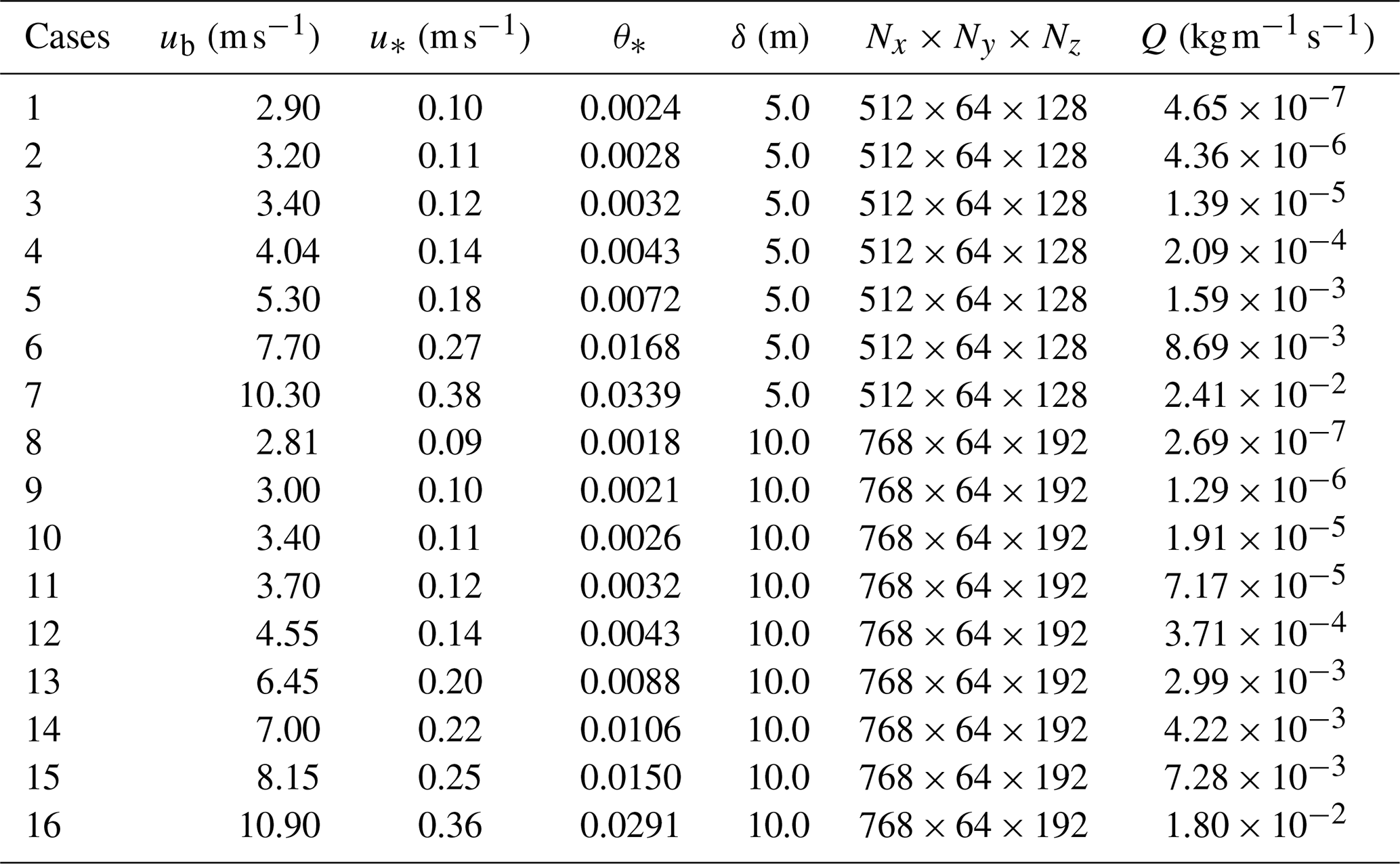
To examine the effect of boundary layer thickness (δ) on near-threshold transport, two cases were simulated with δ=5.0 m and 10.0 m. Results from a smaller domain (δ=1.0 m) partly draw on Jin et al. (2024). The computational domain dimensions are $(L_x\times L_y\times L_z)=(\mathrm{8}\mathit{\pi }\mathit{\delta }\times \mathit{\delta }\times \mathrm{2}\mathit{\pi }\mathit{\delta })$. Grids are uniform in the horizontal direction and stretched vertically using a hyperbolic tangent function with refinement near the wall ($y_{\mathrm{1}}=\mathrm{0.012},\mathrm{0.014}\mathrm{m}$ for δ=5.0 and 10.0 m). For particle field post-processing, identical vertical grid resolution was applied to ensure comparability. Bed particles follow a slightly skewed Gaussian size distribution with a mean diameter of 200 µm (Zhu et al., 2019; Liu et al., 2022b). Particle and air densities are ${\mathit{\rho }}_{\mathrm{p}}=\mathrm{2650}\mathrm{kg}{\mathrm{m}}^{-\mathrm{3}}$ and $\mathit{\rho }=\mathrm{1.2}\mathrm{kg}{\mathrm{m}}^{-\mathrm{3}}$, giving a density ratio of 2208. The α_x and τ_t values are consistent with Jin et al. (2024). Table 1 lists the simulation cases and key parameters.

Table 1 Bulk fluid velocity (u_b), saltation friction velocity (u_∗, effective friction velocity considering particle feedback), Shields number (${\mathit{\theta }}_{\ast }=u_{\ast }^{\mathrm{2}}/\left[\right({\mathit{\rho }}_{\mathrm{p}}/\mathit{\rho }-\mathrm{1}\left)g{d}_{\mathrm{p}}\right])$, boundary layer thickness (δ), grid sizes in three directions ($N_x\times N_y\times N_z$), and sand transport rate (Q) for 16 simulated cases with sediment transport.

3 Results and discussion

This section examines how boundary layer thickness influences near-threshold sand transport. It should be noted that the boundary layer thickness δ not only affects outer-layer structures and inner–outer interactions, but also acts through the friction Reynolds number ${\text{Re}}_{\mathit{\tau }}=u_{\ast }\mathit{\delta }/\mathit{\nu }$. Under the same friction velocity u_∗ and ν, a larger δ corresponds to a higher Re_τ, which supports larger-scale turbulent eddies and richer multi-scale interactions. Therefore, the boundary layer thickness effects observed in this study are essentially manifestations of Reynolds number effects under near-threshold transport conditions.

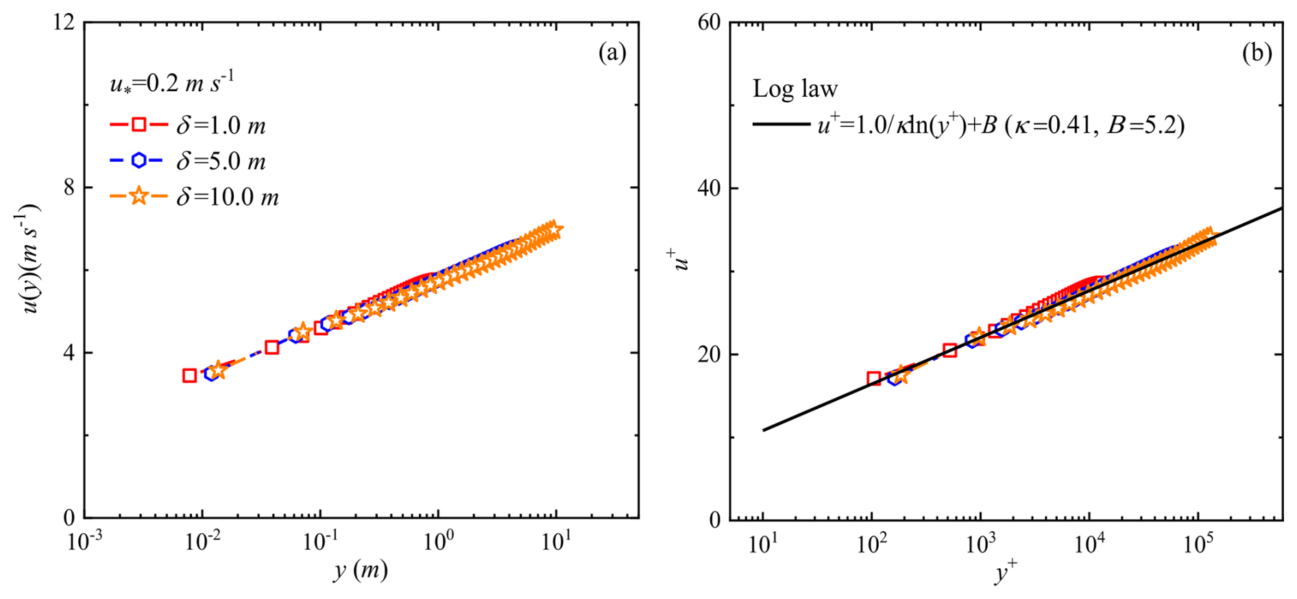
Figure 1 (a) Mean wind velocity profiles u(y) for three boundary layer thicknesses ($\mathit{\delta }=\mathrm{1.0},\mathrm{5.0},\mathrm{10.0}\mathrm{m}$); (b) inner-scale normalized profiles u⁺ compared with the logarithmic law (κ=0.41 is the von Kármán constant and B is taken as 5.5 in the channel, $u_{\mathit{\tau }}=\mathrm{0.21}\mathrm{m}{\mathrm{s}}^{-\mathrm{1}}$).

The simulations span wind velocities from the rebound threshold up to values exceeding the impact entrainment threshold. The rebound threshold in this study refers to the critical condition determined by observing the complete cessation of intermittent saltation motion. It is diagnosed from the simulation results by systematically reducing the wind velocity and observing the complete cessation of all particle motion over a sufficiently long statistical period. Its physical essence is consistent with the critical Shields number defined by Pähtz et al. (2020), which signifies whether sustained particle rebound can be maintained. It should be noted that the determination method differs from the one that estimates the threshold by extrapolating the continuous transport rate to zero. The impact entrainment threshold is identified as the point where the transport regime transitions from intermittent to continuous, corresponding to a marked change in the slope of the transport rate curve.

To reduce computational cost, each numerically resolved particle represents multiple physical particles (Dupont et al., 2013), with the representative ratio ranging from 50–2000 depending on boundary layer thickness and friction velocity. The analysis begins with mean wind velocity profiles and wall-shear stress fluctuations, followed by transport behavior and particle dynamics.

Figure 1a shows mean wind velocity profiles for three boundary layer thicknesses at a fixed friction velocity, plotted in log-linear coordinates. Profiles overlap closely, with only minor differences at the first grid point for the smallest boundary layer. Near-wall velocities remain consistent across all cases, confirming that the first-grid-point height has a negligible influence. Normalizing the profiles using inner scales ($u^{+}=u/u_{\mathit{\tau }},y^{+}=u_{\mathit{\tau }}y/\mathit{\nu }$) (Fig. 1b) shows excellent agreement with the logarithmic law, validating the simulated mean flow fields across boundary layer thicknesses.

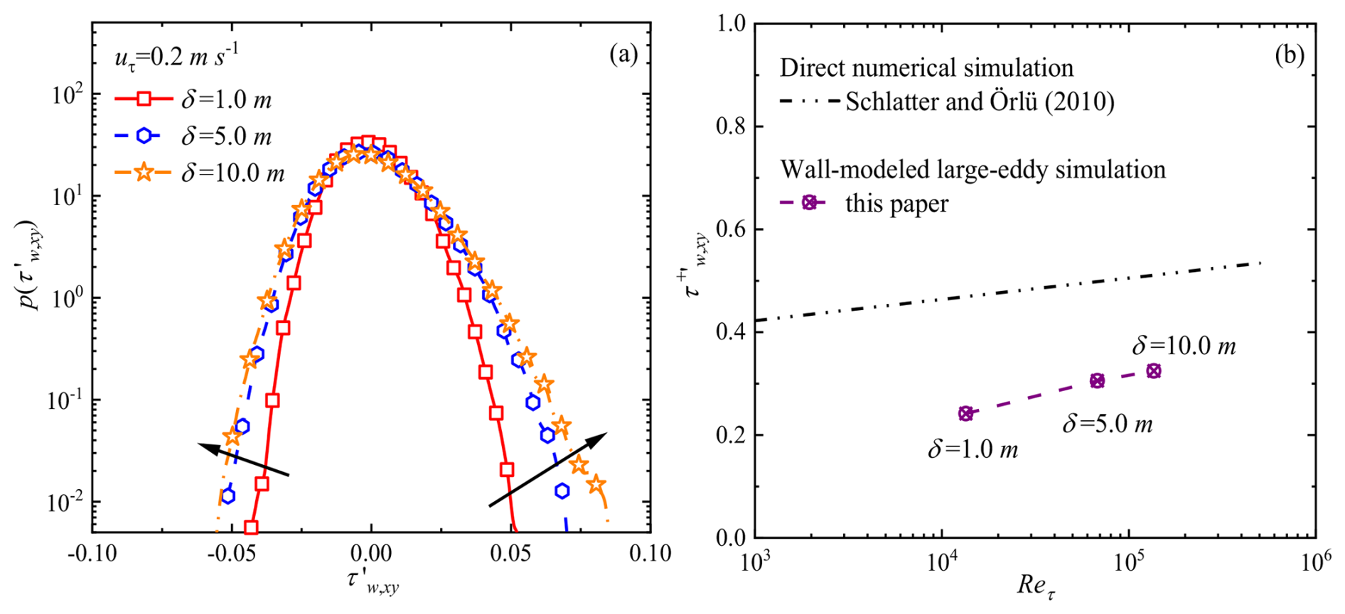
Figure 2 (a) Probability density distributions and (b) standard deviations of wall-shear stress fluctuations ${\mathit{\tau }}_{w,xy}^{\prime }$ for different boundary layer thicknesses ($\mathit{\delta }=\mathrm{1.0},\mathrm{5.0},\mathrm{10.0}\mathrm{m}$). The direct numerical simulation results of Schlatter and Örlü (2010) are given by the double-dash-dotted line.

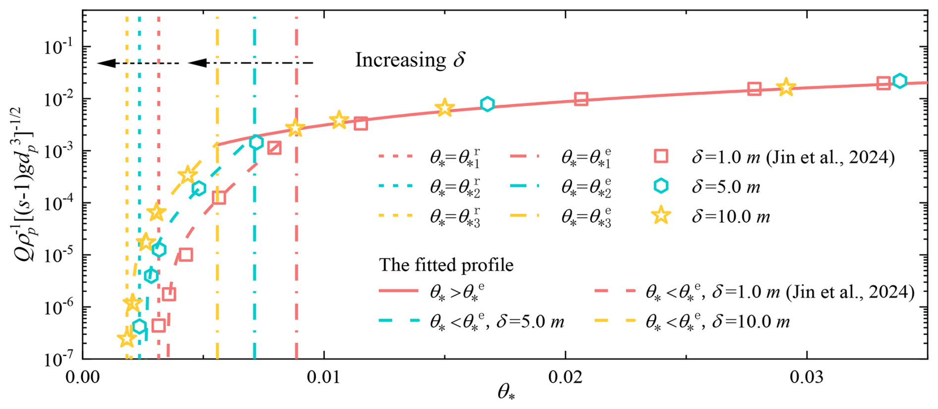
Figure 3 Simulated sand transport rates $Q{\mathit{\rho }}_{\mathrm{p}}^{-\mathrm{1}}\left[\right(s-\mathrm{1})g{d}_{\mathrm{p}}^{\mathrm{3}}{]}^{-\mathrm{1}/\mathrm{2}}$ under different boundary layer thicknesses ($\mathit{\delta }=\mathrm{5.0},\mathrm{10.0}\mathrm{m}$) and wind velocities, where s is the density ratio of particle and air.

Particle liftoff is initiated by instantaneous high shear stresses or local pressure imbalances generated by turbulent fluctuations. Boundary layer thickness influences the velocity threshold for entrainment by modulating near-wall turbulent structures and the resulting wall-shear stress field (Lu et al., 2005; Pähtz et al., 2018). Figure 2a shows the probability density distributions of wall-shear stress fluctuations under the same free-stream wind velocity. The simulations reveal clear differences across boundary layer thicknesses. As the boundary layer increases, the probability densities at both tails of the distribution – especially for positive fluctuations above the mean – also increase. This trend arises because the boundary layer thickness constrains the largest turbulent scales (Pähtz et al., 2018). A thicker boundary layer supports a broader range of turbulent scales, producing stronger instantaneous wall-shear stresses. When the boundary layer thickness increases fivefold (from 1.0–5.0 m), the fluctuation amplitude rises markedly, but further increases lead to a slower rate of growth. Figure 2b compares the standard deviation of wall-shear stress fluctuations with the direct numerical simulation results of Schlatter and Örlü (2010). The lower values obtained here reflect the use of wall-modeled large-eddy simulations with relatively coarse grid resolution. Despite this, the Reynolds number dependence across different boundary layer thicknesses is well captured.

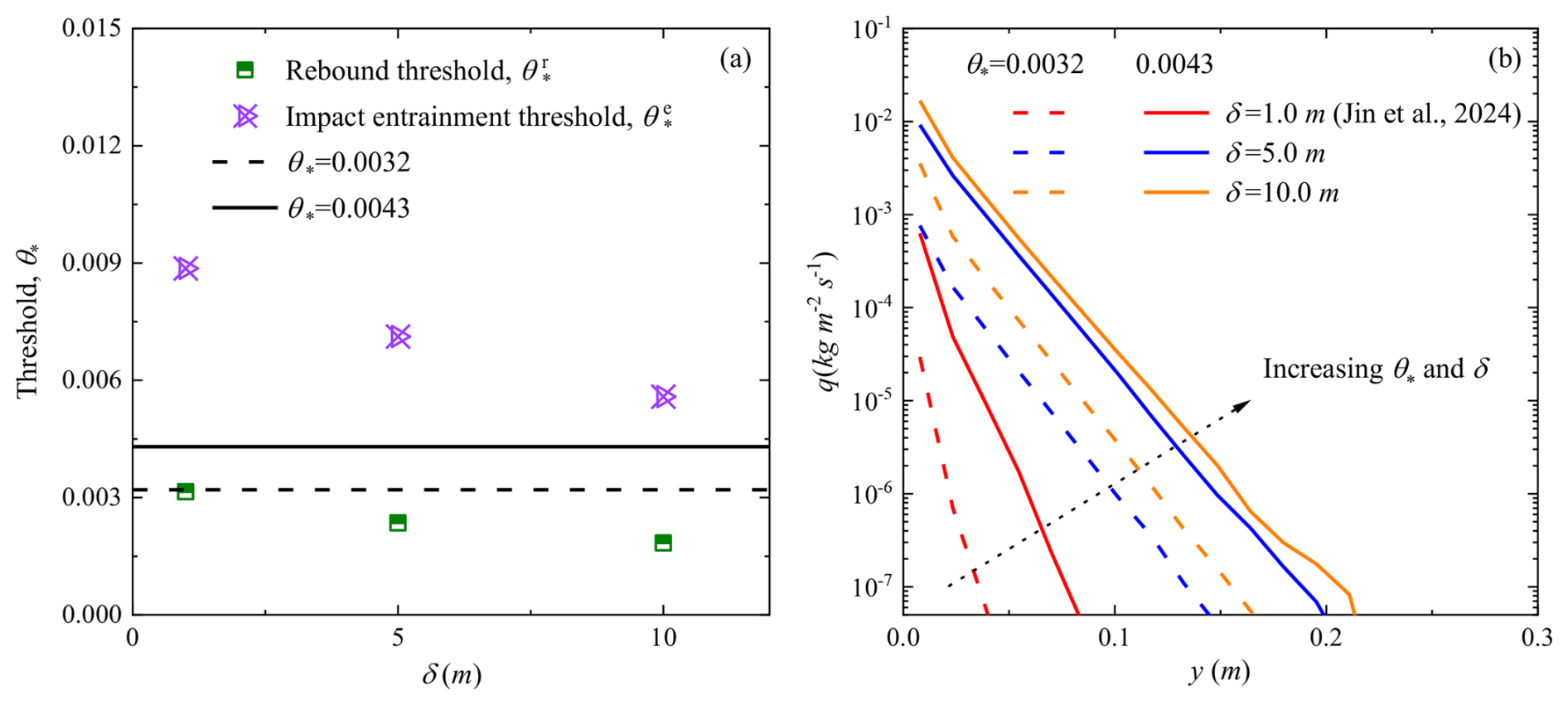
Figure 4 (a) Rebound ${\mathit{\theta }}_{\ast }^{\mathrm{r}}$ and impact entrainment ${\mathit{\theta }}_{\ast }^{\mathrm{e}}$ thresholds and (b) sediment transport intensity q for different boundary layer thicknesses (Data for δ=1.0 m taken from Jin et al., 2024). The dashed line represents ${\mathit{\theta }}_{\ast }=\mathrm{0.0032}$, and the solid line represents ${\mathit{\theta }}_{\ast }=\mathrm{0.0043}$. The color corresponds to different boundary layer thicknesses. The black dotted arrow in (b) represent the increase of boundary layer thickness and wind velocity.

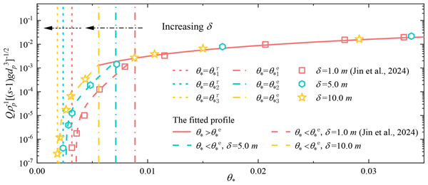
Large-scale turbulent structures carry significant energy and Reynolds stress (Guala et al., 2006; Balakumar and Adrian, 2007), thereby enhancing energy transfer (Marusic et al., 2010; Serafimovich et al., 2011). The influence of boundary layer thickness on these large structures can further affect particle motion in sand-laden flows. Under simulated conditions with δ=1.0 m, Jin et al. (2024) reported that above the impact entrainment threshold (${\mathit{\theta }}_{\ast }^{\mathrm{e}}$), the time-averaged sand transport rate scales shear stress raised to the power of 1.5 (the same as Bagnold, 1941 and White, 1979), whereas below ${\mathit{\theta }}_{\ast }^{\mathrm{e}}$, it varies exponentially with shear stress. As shown in Fig. 3, the simulated sand transport rates across different boundary layer thicknesses and dimensionless wind velocities follow the same trend, with fitted curves yielding a high correlation coefficient (R²). However, the threshold wind velocities depend strongly on the boundary layer thickness. For example, the impact entrainment thresholds required for sustained continuous transport are ${\mathit{\theta }}_{\ast \mathrm{2}}^{\mathrm{e}}=\mathrm{0.00712}$ and ${\mathit{\theta }}_{\ast \mathrm{3}}^{\mathrm{e}}=\mathrm{0.00558}$ for δ=5.0 m and 10.0 m, respectively (dot-dashed lines in Fig. 3). These correspond to impact threshold wind velocities ($u_{\ast }^{\mathrm{e}}$) of 0.18 and 0.16 m s⁻¹, equal to 0.58 and 0.52 times the fluid threshold ($u_{\ast }^t=\mathrm{0.31}\mathrm{m}{\mathrm{s}}^{-\mathrm{1}}$). Similarly, rebound thresholds were ${\mathit{\theta }}_{\ast \mathrm{2}}^{\mathrm{r}}=\mathrm{0.00235}$ and ${\mathit{\theta }}_{\ast \mathrm{3}}^{\mathrm{r}}=\mathrm{0.00184}$ (dashed lines in Fig. 3), corresponding to rebound threshold wind velocities ($u_{\ast }^{\mathrm{r}}$) of 0.1 and 0.09 m s⁻¹, or 0.32 and 0.29 times the fluid threshold.

For a particle size of 200 µm, the threshold coefficient in a fluctuating flow field is about 1.5 times that in the time-averaged flow (Li et al., 2020a). Based on the entrainment threshold of $u_{\ast }^t=\mathrm{0.21}\mathrm{m}{\mathrm{s}}^{-\mathrm{1}}$ obtained from wind tunnel experiments, the rebound thresholds are 47.6 % and 42.9 % of this value, respectively. Field studies also indicate that transport may occur when the friction velocity is just 50 % of the wind-tunnel threshold (Rasmussen and Sørensen, 1999). Given measurement uncertainties and the difficulty detecting particles close to the bed (Jin et al., 2021), the thresholds under field conditions may be even lower than those estimated here. Figure 4a further shows that both ${\mathit{\theta }}_{\ast }^{\mathrm{e}}$ and ${\mathit{\theta }}_{\ast }^{\mathrm{r}}$ decrease with increasing boundary layer thickness, with the decline in ${\mathit{\theta }}_{\ast }^{\mathrm{e}}$ more pronounced. This is consistent with the observation by Williams et al. (1994) that the fluid threshold decreases as turbulence intensifies (effectively equivalent to increasing boundary layer height). Increasing the boundary layer thickness significantly alters the turbulence structure (Li et al., 2020a; Zhang et al., 2022), which modifies the instantaneous probability of exceeding the threshold. This is precisely the physical mechanism underlying the threshold reduction.

Notably, when ${\mathit{\theta }}_{\ast }>{\mathit{\theta }}_{\ast }^{\mathrm{e}}$, the differences in sand transport rates across varying boundary layer thicknesses become negligible. In contrast, when ${\mathit{\theta }}_{\ast }<{\mathit{\theta }}_{\ast }^{\mathrm{e}}$, the sand transport rate scales with the boundary layer thickness and rises sharply with increasing wind velocity (Rasmussen and Sørensen, 1999). For example, at ${\mathit{\theta }}_{\ast }=\mathrm{0.0043}$, the transport rates for δ=5.0 and 10.0 m are 19 and 33 times that for δ=1.0 m, respectively; at ${\mathit{\theta }}_{\ast }=\mathrm{0.0032}$, the corresponding factors increase to 29 and 149, demonstrating that the influence of boundary layer thickness is more pronounced at lower wind velocities. This aligns with the observation made by Williams et al. (1990) that turbulent fluctuations promote entrainment. However, limited by the dimensions of the wind tunnel, the boundary layer thickness in their experiments typically ranges from centimeters to decimeters (corresponding to Re_τ on the order of 10³−10⁴), representing a classic laboratory scale. By systematically extending δ from 1.0–10.0 m in our simulations (with Re_τ reaching ∼105), we have directly bridged the gap between laboratory scales and natural atmospheric scales, where δ is commonly on the order of hundreds of meters.

These findings suggest that in real field conditions, sediment transport rates may be higher and threshold wind velocities lower than predicted in conventional wind tunnels. Feng and Wang (2023) reported a similar trend, observing that sediment transport rates increase with boundary layer thickness at wind velocities (${\mathit{\theta }}_{\ast }>\mathrm{0.15}$, $u_{\ast }>\mathrm{0.8}\mathrm{m}{\mathrm{s}}^{-\mathrm{1}}$ in their study) well above the near-threshold regime considered in this study. This implies that the effect of boundary layer thickness on sediment flux depends on the wind velocity and the dominant particle entrainment mechanism.

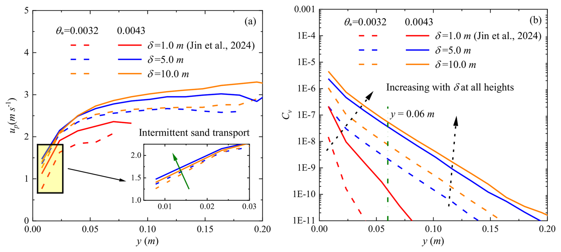
Figure 5 Vertical profiles of (a) mean horizontal particle velocity u_p and (b) particle volume fraction C_v for different boundary layer thicknesses ($\mathit{\delta }=\mathrm{5.0},\mathrm{10.0}\mathrm{m}$). The dashed line represents ${\mathit{\theta }}_{\ast }=\mathrm{0.0032}$, and the solid line represents ${\mathit{\theta }}_{\ast }=\mathrm{0.0043}$. The color corresponds to different boundary layer thicknesses. The green arrow in (a) and the black dotted arrow in (b) represent the increase of boundary layer thickness and wind velocity.

Specifically, at wind velocities below the impact entrainment threshold (${\mathit{\theta }}_{\ast }^{\mathrm{e}}$), thicker boundary layers generate higher instantaneous wall-shear stresses, enhancing fluid-driven particle flux and increasing the sand transport rate. When wind velocities far exceed the impact entrainment threshold (${\mathit{\theta }}_{\ast }>\mathrm{21}{\mathit{\theta }}_{\ast \mathrm{2}}^{\mathrm{e}}or>\mathrm{27}{\mathit{\theta }}_{\ast \mathrm{3}}^{\mathrm{e}}$ according to Feng and Wang, 2023), splash-driven entrainment dominates, and the sand transport flux becomes approximately proportional to the boundary layer thickness. In the transitional wind velocity regime between these limits, both fluid- and splash-driven processes are relatively insensitive to boundary layer thickness, resulting in minimal variation in transport rates.

Sediment transport intensity ($q\left(y\right)=\sum m_{\mathrm{p}}\stackrel{\mathrm{‾}}{u_{\mathrm{p}}}/(L_x\times {\mathrm{\Delta }}_y\times L_z))$, which is defined as the horizontal sand mass flux per unit height interval, serves as a key metric linking the microscopic mechanisms of aeolian sand movement – such as particle entrainment and collisions – to macroscopic outcomes, including the overall sediment transport rate. Using the same grid resolution (grid size of δ=1.0 m), Fig. 4b shows how sediment transport intensity varies with height for different boundary layer thicknesses ($\mathit{\delta }=\mathrm{5.0},\mathrm{10.0}\mathrm{m}$) and dimensionless shear velocities (${\mathit{\theta }}_{\ast }=\mathrm{0.0032},\mathrm{0.0043}$). For comparison, simulation results for δ=1.0 m (Jin et al., 2024) are also included to highlight the combined effects of wind velocity and boundary layer thickness. All profiles exhibit an exponential decay with increasing height.

As illustrated in Fig. 4a, the selected wind velocities (${\mathit{\theta }}_{\ast }=\mathrm{0.0032},\mathrm{0.0043}$) are above the rebound threshold but below the impact entrainment threshold for all three boundary layer thicknesses, indicating that sediment transport occurs intermittently under these conditions. As both wind velocity and boundary layer thickness increase, the sediment transport intensity rises across all heights, with differences becoming more pronounced at greater heights. The effect of boundary layer thickness is particularly significant at lower wind velocities. For instance, at a height of y=0.04 m, the sediment transport intensity for δ=5.0 and 10.0 m increases by approximately 1000 and 3000 times, respectively, relative to δ=1.0 m at ${\mathit{\theta }}_{\ast }=\mathrm{0.0032}$. At ${\mathit{\theta }}_{\ast }=\mathrm{0.0043}$, the corresponding increases are about 100 and 150 times, indicating that the influence of boundary layer thickness diminishes as wind velocity increases. Importantly, the variations in sediment transport intensity due to boundary layer thickness at this height are far larger than those observed in the total transport rate, since the sediment transport intensity for δ=1.0 m is relatively low and contributes only minimally to the overall flux.

Figure 5a shows the vertical profile of mean horizontal particle velocity. Unlike continuous transport conditions – where wind velocities exceed the impact entrainment threshold and thicker boundary layers generally result in faster particle movement at the same wind velocity (Feng and Wang, 2023) – the relationship under sub-threshold conditions is non-monotonic. At different wind velocities, particle velocity for δ=1.0 m is lower than for δ=5.0 m, but shows little change when the boundary layer thickness increases further to δ=10.0 m. As wind velocity rises, the velocity difference between δ=1.0 m and δ=5.0 or 10.0 m diminishes. Simulation results for δ=5.0 and 10.0 m also demonstrate that near-wall particle velocity is proportional to wind velocity (see inset of Fig. 5a), confirming that sediment transport remains intermittent when ${\mathit{\theta }}_{\ast }<\mathrm{0.0043}$ (Jin et al., 2024). However, greater boundary layer thickness leads to smaller velocity variations across different wind velocities under thicker boundary layers.

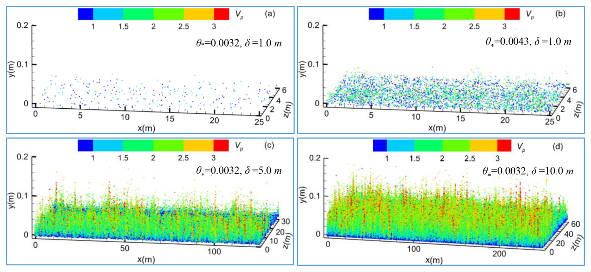
Figure 6 Instantaneous particle fields V_p for different boundary layer thicknesses ($\mathit{\delta }=\mathrm{1.0},\mathrm{5.0},\mathrm{10.0}\mathrm{m}$) and wind velocities: (a) ${\mathit{\theta }}_{\ast }=\mathrm{0.0032}$, δ=1.0 m; (b) ${\mathit{\theta }}_{\ast }=\mathrm{0.0043}$, δ=1.0 m; (c) ${\mathit{\theta }}_{\ast }=\mathrm{0.0032}$, δ=5.0 m; (d) ${\mathit{\theta }}_{\ast }=\mathrm{0.0032}$, δ=10.0 m, where data for δ=1.0 m come from Jin et al. (2024). The resultant velocity V_p is equal to the square root of the sum of the squares of the velocities in the three directions.

Feng and Wang (2023) observed that particle volume fraction increases with boundary layer thickness only in regions far from the wall (e.g., y>0.06 m when ${\mathit{\theta }}_{\ast }=\mathrm{0.0427}$). In contrast, the present results show that under the same wind velocity, particle volume fraction is proportional to boundary layer thickness across all heights (Fig. 5b). This discrepancy arises due to the predominance of fluid-driven particle entrainment under low wind velocities rather than splash events. These fluid-driven particles move at lower velocities, and only a small fraction gains sufficient energy to reach the saltation layer. Consequently, near-wall particle concentration exhibits a strong dependence on boundary layer thickness. Supporting this, Jin et al. (2024) showed for δ=1.0 m that when ${\mathit{\theta }}_{\ast }=\mathrm{0.0032}$ (very close to the rebound threshold), the transport flux is almost entirely carried by fluid-driven particles. Because such particles have much lower energy than splash-entrained ones, their flux decays rapidly with height. As wind velocity and boundary layer thickness increase – where a thicker boundary layer at the same wind velocity corresponds to a larger argin above the rebound threshold – the decay rate of particle flux with height decreases progressively.

As wind velocity approaches the rebound threshold, the height of particle saltation decreases. To illustrate how particle distributions vary with wind velocity and boundary layer thickness, Fig. 6 shows instantaneous particle fields at a representative moment after the aeolian sand flow has reached a steady state for δ=1.0 m (${\mathit{\theta }}_{\ast }=\mathrm{0.0032},\mathrm{0.0043}$), δ=5.0 m (${\mathit{\theta }}_{\ast }=\mathrm{0.0032}$), and δ=10.0 m (${\mathit{\theta }}_{\ast }=\mathrm{0.0032}$). Particle colors denote velocity, and each plotted particle represents 50 actual particles. For δ=1.0 m at ${\mathit{\theta }}_{\ast }=\mathrm{0.0032}$, the maximum saltation height is about 0.03 m (roughly 150 particle diameters), indicating weak sand transport (Fig. 6a). Particle motion is confined to creep or short saltation near the wall, with particle detachment relying primarily on turbulent fluctuations rather than interparticle collisions. As wind velocity increases (${\mathit{\theta }}_{\ast }=\mathrm{0.0043}$, Fig. 6b), particle motion intensifies, velocities rise, and the aeolian sand flow develops more rapidly with increasing boundary layer thickness. Under δ=10.0 m, the maximum saltation height approaches 0.2 m. Statistical results confirm that at higher wind velocities, increases in flux are dominated by higher particle concentrations (Fig. 5).

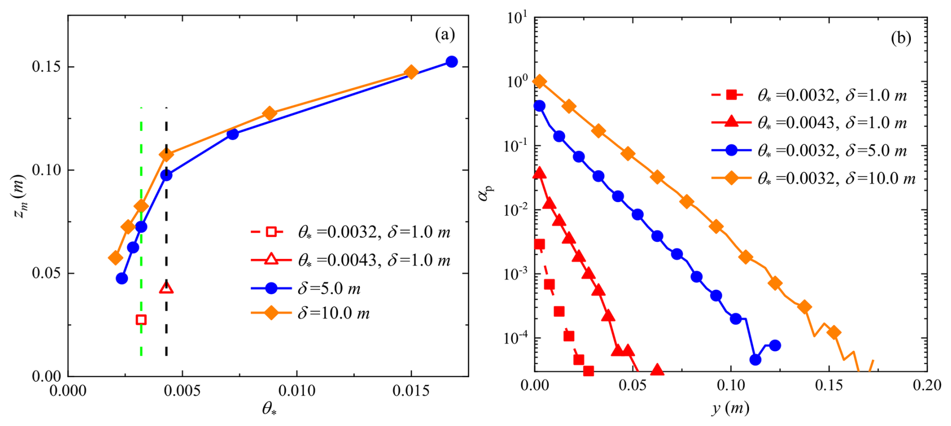
Figure 7 (a) Saltation layer height z_m and (b) particle spatial occupancy α_p for different boundary layer thicknesses ($\mathit{\delta }=\mathrm{5.0},\mathrm{10.0}\mathrm{m}$) and wind velocities. The green and black dashed lines in (a) are auxiliary lines for ${\mathit{\theta }}_{\ast }=\mathrm{0.0032}$ and 0.0043.

The saltation layer height z_m was also extracted (Fig. 7a), defined as the elevation below which 99.5 % of the total mass flux occurs (Dupont et al., 2013). At wind velocities of ${\mathit{\theta }}_{\ast }=\mathrm{0.0032}$ and 0.0043, the saltation layer thickness for δ=10.0 m is approximately 3.0 and 2.5 times greater than for δ=1.0 m, respectively. As wind velocity increases further, the differences among boundary layer thicknesses diminish, especially for δ=5.0 m and δ=10.0 m.

To quantify the non-uniformity of particle distributions, we define the particle spatial occupancy (α_p) as the ratio of grid cells containing particles to the total number of grid cells. Using the instantaneous particle fields shown in Fig. 6, Fig. 7b presents the vertical variation of α_p under different conditions at the same grid resolution. The results show that α_p decays exponentially with increasing height, reflecting its close relationship to the vertical distribution of particle volume fraction. Near the wall, α_p for δ=10.0 m approaches 1, indicating nearly complete grid-cell occupancy. Under the same wind velocity, α_p for δ=5.0 m decreases to ∼ 0.4, indicating spatial heterogeneity in particle distribution, while for δ=1.0 m, α_p falls sharply to 0.003, signifying strong spatial variability with particles confined to localized regions of the flow.

Increasing boundary layer thickness markedly enhances energy transfer between the turbulent flow and the particle phase. Large-scale vortices in thicker boundary layers carry greater energy and persist longer, which promotes more effective and sustained particle lifting, resulting in both vertical and horizontal dispersion and thus a more uniform distribution and significantly higher α_p values. Moreover, the effect of boundary layer thickness on α_p increases with increasing height above the wall (Fig. 7b).

Furthermore, taking the near-threshold wind velocity (${\mathit{\theta }}_{\ast }=\mathrm{0.0032}$) as an example, we selected three different domains (all centered within the computational domain): 0.05 m×0.05 m, 0.1 m×0.1 m, and 0.2 m×0.2 m. Within these finite horizontal domains, we present the fraction of time f_Q for which saltation is in an “active” state over a given analysis time window Δt(2 s), as defined by Martin and Kok (2018), based on a total time series exceeding 60 s (Fig. 8). It can be seen that for the thin boundary layer (δ=1.0 m), f_Q approaches zero in any of the finite domains, whereas for the thick boundary layers (δ=5.0 m and 10.0 m), f_Q is close to 1 in all finite domains. This demonstrates that, in near-threshold large-scale simulations, f_Q is severely constrained by the stark dichotomy of transport states. Therefore, in the present study, α_p is adopted to compare the tendency of particle transport toward spatial dispersion or clustering under different boundary layer thicknesses – precisely the kind of global structural information that the spatiotemporal metric f_Q is inherently unable to capture.

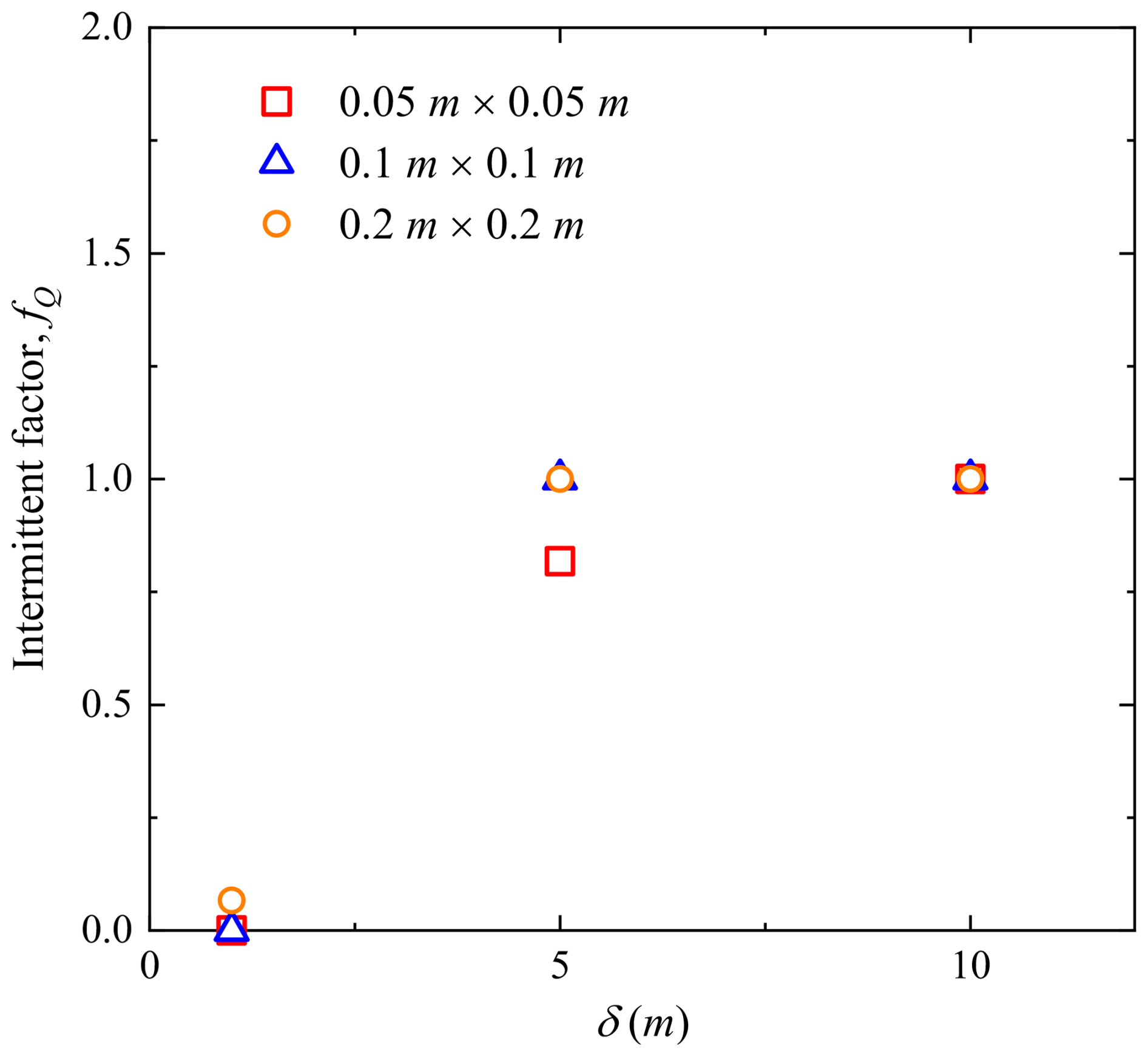
Figure 8 Fraction of time f_Q for which saltation is in an “active” state under different boundary layer thicknesses (${\mathit{\theta }}_{\ast }=\mathrm{0.0032}$).

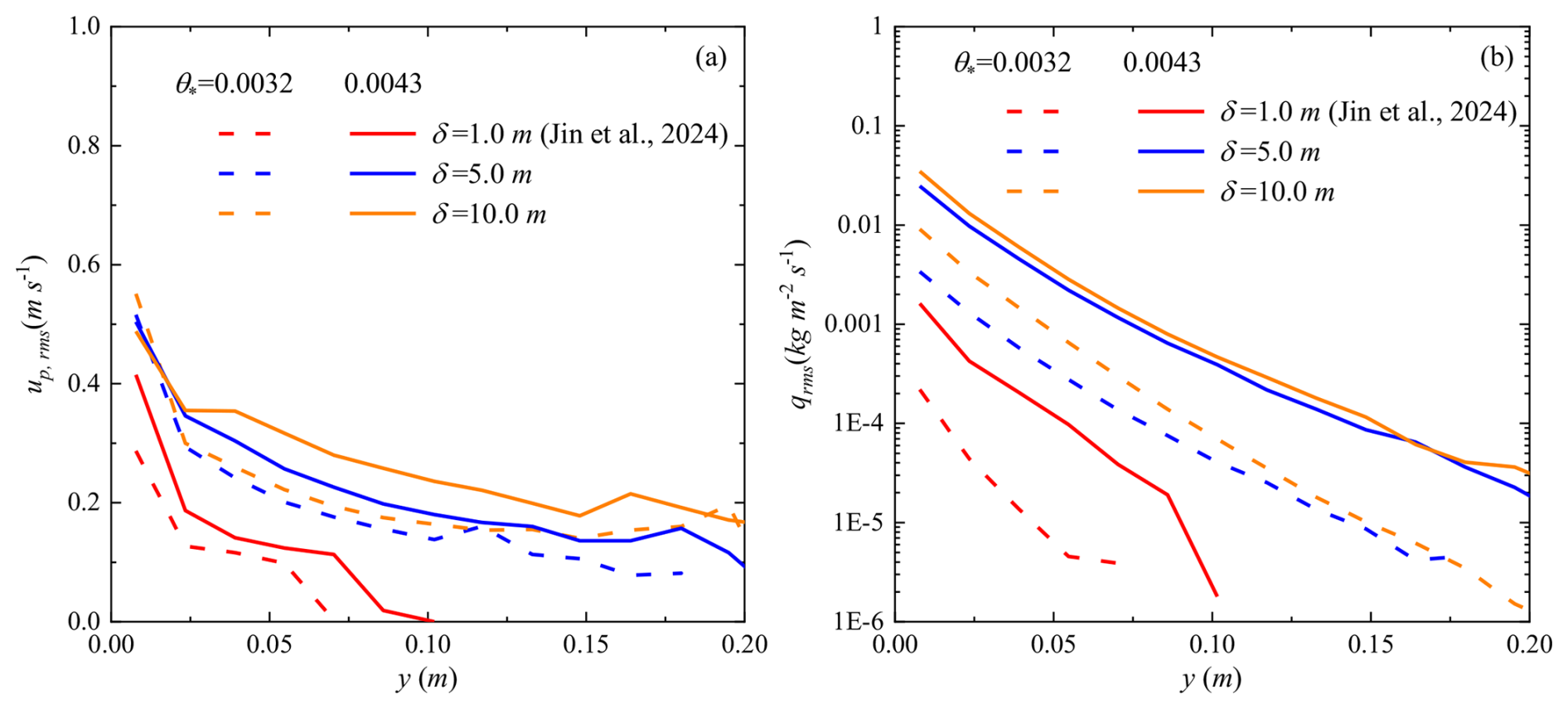
Figure 9 Vertical profiles of (a) particle velocity u_p,rms and (b) mass flux q_rms fluctuations for different boundary layer thicknesses ($\mathit{\delta }=\mathrm{5.0},\mathrm{10.0}\mathrm{m}$). The dashed line represents ${\mathit{\theta }}_{\ast }=\mathrm{0.0032}$, and the solid line represents ${\mathit{\theta }}_{\ast }=\mathrm{0.0043}$. The color corresponds to different boundary layer thicknesses.

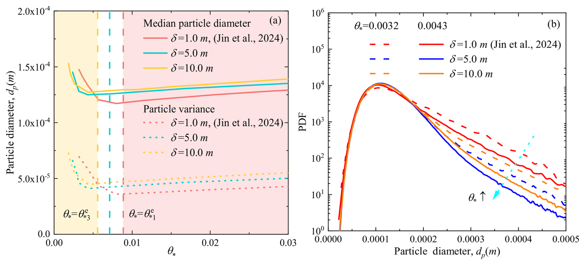
Figure 10 (a) Mean and variance, and (b) probability density distribution of particle diameter d_p for different boundary layer thicknesses ($\mathit{\delta }=\mathrm{5.0},\mathrm{10.0}\mathrm{m}$) as a function of wind velocity. The median particle diameter is represented by solid lines, and the variance of particle diameter is represented by dashed lines in (a). The line types and colors in (b) are consistent with those in Figs. 5 and 9. The arrows in (b) indicate that as the wind velocity increases, the probability density of large particles (those with larger diameters) decreases.

Figure 9 presents the vertical profiles of particle velocity and mass flux fluctuations. Even when the boundary layer thickness increases to 5.0 and 10.0 m, the peak of particle velocity fluctuations remains located in the near-wall region. This near-wall concentration of fluctuations can markedly intensify wind erosion under low wind velocity conditions. It also reinforces the prevalence of the intermittent transport regime, dominated by fluid-driven entrainment, which differs from the continuous saltation dominated by splash-driven entrainment, where the velocity fluctuation peak typically occurs several centimeters above the bed (Feng and Wang, 2023). Across all simulated wind velocities, increasing the boundary layer thickness from 1.0–5.0 m significantly amplifies the near-wall velocity fluctuation peak, a phenomenon closely related to the intensification of outer large-scale structures and their influence on the inner region (Smits et al., 2011). However, further increases to 10.0 m produces little additional change, suggesting a gradual transition toward splash-driven entrainment. Differences in velocity fluctuations associated with boundary layer thickness become more apparent only at higher elevations above the wall.

Mass flux fluctuations near threshold also differ from those in continuous transport. As shown in Fig. 9b, as the boundary layer thickness increases, the magnitude of transport rate fluctuations rises but the incremental effect diminishes, particularly at higher wind velocities. Consequently, the influence of boundary layer thickness on mass flux fluctuations weakens as wind velocity increases. This behavior mirrors the response of the mean sediment transport rate, reflecting the fact that as wind velocity approaches the splash-driven entrainment threshold, both fluid- and splash-driven processes become less sensitive to variations in boundary layer thickness.

Under conditions with boundary layer thicknesses $\mathit{\delta }=\mathrm{5.0},\mathrm{10.0}\mathrm{m}$ (Fig. 10a), the variation of particle diameter parameters reveals two distinct regimes. When wind velocity is below the impact entrainment threshold (${\mathit{\theta }}_{\ast }^{\mathrm{e}}$), both the mean and variance of airborne particle diameter decrease with increasing θ_∗. In contrast, once wind velocity exceeds ${\mathit{\theta }}_{\ast }^{\mathrm{e}}$, both parameters become proportional to θ_∗, consistent with the conclusions drawn for δ=1.0 m and supporting the validity of defining the critical threshold based on transport rate. At lower wind velocities, the relationship between mean and variance differs across boundary layer thicknesses: $d_{\mathrm{p},\mathit{\delta }=\mathrm{1.0}\mathrm{m}}>d_{\mathrm{p},\mathit{\delta }=\mathrm{5.0}\mathrm{m}}>d_{\mathrm{p},\mathit{\delta }=\mathrm{10.0}\mathrm{m}}$. Conversely, thicker boundary layer thicknesses result in greater mean and variance. The simulation results indicate the existence of two critical Shields numbers: ${\mathit{\theta }}_{\ast \mathrm{1}}=\mathrm{0.003}$ and ${\mathit{\theta }}_{\ast \mathrm{2}}=\mathrm{0.005}$. The shift in the particle statistics relationship corresponds to θ_∗1 when comparing δ=10.0 m with δ=5.0 m, and to θ_∗2 when comparing $\mathit{\delta }=\mathrm{5.0},\mathrm{10}\mathrm{m}$ with δ=1.0 m. For wind velocities of ${\mathit{\theta }}_{\ast }=\mathrm{0.0032}$ and 0.0043, lying between these two critical values, the relationship between mean and variance shifts accordingly: $d_{\mathrm{p},\mathit{\delta }=\mathrm{1.0}\mathrm{m}}>d_{\mathrm{p},\mathit{\delta }=\mathrm{10.0}\mathrm{m}}>d_{\mathrm{p},\mathit{\delta }=\mathrm{5.0}\mathrm{m}}$, as also confirmed by the probability density distributions in Fig. 10b.

As wind velocity increases (θ_∗ rising from 0.0032 to 0.0043), the probability of entraining larger particles decreases because both ${\mathit{\theta }}_{\ast }=\mathrm{0.0032}$ and 0.0043 remain below ${\mathit{\theta }}_{\ast }^{\mathrm{e}}$, meaning that fluid-driven entrainment still dominates particle transport. Under these conditions, the enhanced near-wall transport flux induces a reduction in local wind velocities due to particle loading (Jin et al., 2021), which further suppresses the fluid entrainment of larger particles.

4 Discussion and conclusions

Unlike atmospheric stability (convective/stable conditions), which modify the generation mechanisms and energy distribution patterns of turbulence, the boundary layer thickness not only constrains the maximum possible scale of vortical structures in turbulent motion, but also affects the near-wall turbulence characteristics through the interaction between the inner-outer interactions (Guala et al., 2006; Marusic et al., 2010). Increasing δ corresponds to an expansion of the flow domain in the vertical direction, allowing for the generation and development of larger-scale, more energetic coherent structures. By fixing other flow parameters (the kinematic viscosity, the mean wall friction velocity, the boundary conditions, and the manner in which the inflow turbulence is initialized), this study highlights the influence of boundary layer thickness in modulating near-threshold aeolian sediment transport, a process characterized by high intermittency. A thicker boundary layer supports large-scale coherent structures, such as low-speed streaks or streamwise vortex pairs. These structures induce high instantaneous shear stresses in the near-wall region. Even when the mean shear stress is low, once this instantaneous stress exceeds the fluid threshold, it can trigger localized burst-like particle motion, thereby dominating the intermittent transport behavior.

Recognizing that traditional models, often assuming steady, continuous sediment transport governed by a single threshold (Kawamura, 1951; White, 1979; Creyssels et al., 2009), fail to capture near-threshold behavior, this research addresses a critical knowledge gap. The primary objective is to systematically elucidate how different boundary layer conditions influence the turbulent flow field and the resulting particle entrainment and transport mechanisms near threshold. To achieve this, the study employs the three-dimensional large-eddy simulation coupled with a Lagrangian saltation model, aiming to provide a mechanistic understanding of wind tunnel-field discrepancies.

Increasing boundary layer thickness enhances extreme values in wall-shear stress fluctuations. As a result, both the impact entrainment threshold (${\mathit{\theta }}_{\ast }^{\mathrm{e}}$ or $u_{\ast }^{\mathrm{e}}$) and the rebound threshold (${\mathit{\theta }}_{\ast }^{\mathrm{r}}$ or $u_{\ast }^{\mathrm{r}}$) decrease. For thick boundary layers (δ=5.0 and 10.0 m), the rebound threshold wind velocity can drop below 50 % of values typically observed in conventional wind tunnel experiments. Sediment transport responds differentially to wind velocity: at very low wind velocities (${\mathit{\theta }}_{\ast }^{\mathrm{r}}<{\mathit{\theta }}_{\ast }<{\mathit{\theta }}_{\ast }^{\mathrm{e}}$), transport increases markedly with thickness under fluid-driven entrainment; at high wind velocities (${\mathit{\theta }}_{\ast }>\mathrm{21}{\mathit{\theta }}_{\ast \mathrm{2}}^{\mathrm{e}}$ or $>\mathrm{27}{\mathit{\theta }}_{\ast \mathrm{3}}^{\mathrm{e}}$), it scales proportionally with thickness under splash-driven entrainment; and at intermediate wind velocities, the effect is negligible. Near-bed particle velocity, concentration, saltation height, and airborne particle diameter all increase with boundary layer thickness, accompanied by reduced variability and more uniform spatial distributions.

A thicker boundary layer accommodates a broader range of turbulent scales, fostering stronger, large-scale coherent structures that generate more extreme instantaneous stress events (Pähtz et al., 2018). This enhanced turbulence facilitates particle entrainment at lower mean wind velocities, which also explains why the rebound threshold can be less than half the typical wind-tunnel value (Rasmussen and Sørensen, 1999). Notably, the impact entrainment threshold exhibits a more pronounced reduction, implying that sustaining continuous transport becomes feasible at relatively lower velocities as boundary layer thickness increases. Furthermore, the dependence of sand transport on boundary layer thickness reveals distinct regimes: at low winds, enhanced turbulent fluctuations directly loft more particles, while at high winds, the system transitions to a splash-dominated regime where transport capacity scales with the thicker boundary layer (Feng and Wang, 2023).

Thicker boundary layers promote more energetic large-scale turbulent structures that effectively lift and disperse particles, leading to a more uniform distribution and reduced variability. This mechanism explains previous field observations of longer and more persistent “streamers” (Baas and Sherman, 2005; Sherman et al., 2013). Unlike the findings of Feng and Wang (2023), which showed increased concentration only away from the wall, our results reveal the unique nature of the near-threshold, fluid-entrainment-dominated regime. The observed reversal in particle size trend is due to the shift from fluid-driven to splash-driven entrainment.

Convective boundary layers can reach thicknesses of 1–2 km, neutral boundary layers are typically on the order of hundreds of meters, and stable boundary layers may contract to tens of meters. The range of thicknesses simulated in this study precisely spans the transitional interval from typical wind tunnel scales (approximately 0.1 m) to natural atmospheric scales (>100 m), providing a crucial mechanistic explanation for understanding the systematic differences in sediment transport thresholds and rates between wind-tunnel and field observations. Although this study reveals the significant influence of boundary layer thickness on near-threshold aeolian sediment transport, several issues require further investigation in the future, such as a thicker boundary layer (closer to realistic atmospheric conditions) and a broader particle size distribution to clarify the underlying mechanisms systematically. The current model does not account for multiphysical processes, such as interparticle collisions, electrostatic interactions, or humidity effects, which significantly influence the entrainment and transport of fine particles in natural environments. A logically crucial and necessary step is to adopt the CFD–DEM framework – under conditions that can resolve large-scale flow fields while incorporating realistic particle–particle and particle–bed interactions – to verify, refine, and extend the findings obtained in this study based on a macroscopic parameterized model. What's more, spectral methods or higher-order numerical schemes will also be a key direction for future improvement.

Our findings fundamentally shift how the atmospheric boundary layer should be viewed in dust emission modeling. By demonstrating that thicker boundary layers can halve the entrainment thresholds and alter particle size distributions, we provide the mechanistic basis for the known discrepancy between wind-tunnel models and field observations. This implies that current climate models likely underestimate dust emissions. Integrating boundary layer thickness into dust emission schemes is therefore critical for accurate simulation of aerosol radiative forcing, cloud processes, and the evolution of arid landscapes in a changing climate.