Automated detection of low-altitude isolated mesospheric radar echoes using YOLOv8: evidence for an ionospheric “C layer” phenomenon below 60 km altitude?

The Earth's ionosphere is created by incident solar radiation and extends from approximately 60 to 800 km altitude. Within the ionosphere distinct regions are formed based on the number density of the dominant chemical species and their ionisation by the incident solar ultraviolet radiation and X-rays. The generally accepted lowermost ionospheric region is called D region and extends during daytime from, for example, 90 km downwards to approximately 60 km. Previous studies suggested the presence of an ionospheric C layer around 60 km mostly for observations at very low frequencies. In recent years, rather faint echoes from below the typically altitude-continuous D region have been observed during the sunlit period using a monostatic 3.17 MHz ground-based radar system at polar latitudes. The aim of this study is to distinguish radar echoes from altitudes near 60 km from regular D region echoes and attribute them to a possible C layer source. To our knowledge, this study might be the first systematic investigation of such a phenomenon through monostatic radar observations. Following an initial manual inspection of the raw data and the corresponding radar image spectra, an automated deep learning approach was developed and employed to detect these isolated low-altitude echoes. We used the pattern recognition tool YOLO (You Only Look Once) to gain statistical information on the occurrence of these radar echoes over four years of radar measurements, which covered conditions ranging from minimum to maximum solar activity. The median altitude of these radar echoes is found to be 58.5 km (σ=3.9 km), a thickness of ≈ 6 km per layer, and where the majority of detections exhibit a relatively narrow power spectrum. Substantial annual variability was found for these parameters and the occurrence rate, essentially separating them into summer and winter. The reduced occurrence rates during the solar maximum year 2024 and with that also a reduced intensity of galactic cosmic rays (GCR) suggest their role as an ionisation source for the observed layers.

1 Introduction

With the presence of incident solar radiation, mainly ultraviolet (UV, Lyman-alpha) and X-rays, the ionosphere is formed as atoms and molecules in the Earth's upper atmosphere are ionised. With the ionisation of mostly nitrogen, oxygen as well as nitric oxide, free electrons are created that accumulate in certain ionospheric regions (see e.g. Hargreaves, 1992; Schunk and Nagy, 2009). The layers within the regions vary in intensity and peak heights with diurnal, annual and (multi-) decadal periodicities. The general understanding is, that the layers stretch from the D region at the bottom (≈ 60–90 km) to the E region (≈ 90–120 km) and on to the F region (≈ 150–800 km). All of these regions and their variability play a significant role in radio wave propagation from very low frequencies of a few tens of kHz up to the microwave range of several GHz.

The upper regions (E and F) are monitored by various radar systems, but the most continuous and systematic approach is the Ionosonde HF sounder, probing the ionosphere for many decades with radar frequencies of typically 1–10 MHz (see e.g. Galkin et al., 2006). These systems are used to gain information about the electron density in these regions and layers within, but also allow long-term analysis of its variability (see e.g. Sivakandan et al., 2025). Predominantly for these regions above 100 km altitude, the International Reference Ionosphere Model (IRI, see e.g. Bilitza et al., 2022) is used when measurements are not available.

The ionospheric D region is primarily formed by solar extreme ultraviolet radiation (Lyman-alpha) but also by X-rays during solar active periods (see e.g. Nicolet and Aikin, 1960; Nestorov, 1965; Mitra, 1978; Pavlov, 2014; Friedrich, 2016). This lowermost part of the ionosphere (D region and possibly below) is generally less well monitored because its electron density is lower, and therefore also the gradients are much smaller, which limits the available measurement techniques. In situ measurements with sounding rocket payloads have contributed significantly, but are limited in spatial and temporal coverage (e.g. Friedrich et al., 2017). In the recent years, the monitoring of very low frequency (VLF) transmissions have gained popularity to infer the D region situation (e.g. Siskind et al., 2018).

Another option is the observation with medium or high frequency partial reflection (PR) radars (see e.g. Reid, 2015), which can be used to measure the dynamics as well as the electron density within the D region (e.g. Renkwitz et al., 2018, 2023, for the same radar used in this study).

For middle latitudes this ionisation process forms a Chapman function layer, which facilitates the required radio refractive index. The altitude of maximum echo power seen by a PR radar may vary depending on the local time or, more precisely, on the solar zenith angle (see e.g. Holdsworth and Reid, 1997; Holdsworth et al., 2001; Reid, 2015, Fig. 13a and further references within this review). For solar and geomagnetic quiet periods the maximum echo power at high latitudes is typically detected at 80–90 km altitude (see e.g. Schlegel et al., 1978; Tsutsumi et al., 2001; Singer et al., 2011; Renkwitz and Latteck, 2017).

PR radar echoes from altitudes from the lower mesosphere, as low as 60 km, are in fact not rare (see e.g. Gardner and Pawsey, 1953; Belrose and Burke, 1964; Thrane et al., 1968; Schlegel et al., 1978; Holdsworth and Reid, 1997; Singer et al., 2011; Renkwitz et al., 2018), but these often belong to the altitude-continuous D region structure. This means, that in a coarse picture the D region electron density and its stratification gradually increases during local noon time from 60 to 85 km and with this also the possibility of sufficiently large gradients.

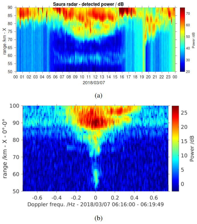
Figure 1 (a) Detected power of the Saura radar for 7 March 2018 showing an intense and long-lasting example of a low-altitude isolated mesospheric radar echo (LIME) at about 58 km altitude and the regular D region echoes above. (b) Example of an image power spectrum for the same experiment and day as in (a).

At high latitudes the occurrence of energetic particle precipitation (EPP) may easily alter the ionisation state of the D region (see e.g. Mironova et al., 2015). In such scenarios, the electron density in the lower D region is significantly enhanced quite rapidly, which then allows pronounced echoes from altitudes of about 60 km and partly below. At the same time, however, this also leads to severe absorption of the radar waves at higher altitudes (see e.g. Hargreaves, 1992). During such events, the typical D region echoes disappear, which makes the EPP related echoes appear as isolated layers. This phenomenon has been reported by Hall et al. (2006) for the medium frequency (MF) radars in Tromso (70° N, 19° E) as well as for extreme scenarios for Saskatoon (52° N, 107° W). Similarly, Kawamura et al. (2007) reported the same type of echoes for the MF radar in Poker Flat, Alaska. Hall et al. (2006) called the observed radar echoes “Isolated Lower Mesospheric Echoes” (ILME) and related most of their observations to solar proton events. Thus also the detected altitudes reached around 50 km. Later, Renkwitz and Latteck (2017) reported on EPP events as observed with the Saura and the nearby Andenes MF PR radar. This study included the daily, annual and decadal occurrences as seen with the Saura PR radar between 2003 and 2016. Contrary to Hall et al. (2006), Renkwitz and Latteck (2017) removed solar proton events, which typically represent extreme D region ionisation scenarios. In Renkwitz and Latteck (2017) is also demonstrated the connection between ILME and VHF radar echoes that are known as Polar Mesospheric Winter Echoes (PMWE), which was followed up in more detail in Renkwitz et al. (2021).

For the southern polar latitudes, simultaneous observations of ILME and PMWE with MF and VHF radars during strong geomagnetic disturbances have been reported by Morris et al. (2011) and Nishiyama et al. (2018).

These EPP-related events (ILME) are very prominent in the radar power profiles, with the maximum detected power being measured at about 60 km, whilst above this altitude there is excessive radar wave absorption, causing the typical D region to disappear.

The term “C layer” was introduced to interpret observations of VLF and LF propagations, for which a certain amount of electron density was expected to be present near 60 km altitude (see e.g. Krasnushkin, 1962; Bain and May, 1967; Bain, 1982; Bain and Kossey, 1987) and more recently by Bertoni et al. (2013). Bertoni et al. (2013) analysed VLF network observations and relate them to the presence of a C layer of enhanced electron densities near 64 to 68 km for a few hours after sunrise. The estimates of required electron densities ranged from 10–100 cm⁻³, which is in good agreement to sounding rocket experiments (see e.g. Friedrich et al., 2018). As the D region may extend to such altitudes around local noon, existing gradients might actually be already large enough to also explain some of the observed VLF propagation. For observations near sunrise and sunset, however, the D region should still be absent at lower altitudes.

More recent radar observations at the boundary of MF and HF range, however, showed the recurring presence of rather faint echoes that are well isolated from the D region signals. Figure 1a depicts one such event, showing a very persistent echoing layer at around 58 km that is clearly separated from the typical D region echoes. Vertically extended enhancements with similar detected power are caused by interference from other transmitters. A corresponding spectrum is shown in Fig. 1b for one experiment (≈ 220 s duration) of the same day. The type of radar echoes reported in this manuscript is not related to EPP, with its intense ionisation enhancements. We focus on radar echoes that occur during geomagnetic and solar quiet conditions, during which the daytime D region radar echoes are visible. Thin and usually faint radar echoes are occasionally observed below and clearly isolated to the normal D region. With the term “isolated” we refer to the drop of detected power to the noise floor above those echoes before the continuous D region starts with increasing echo power. These layers seem to form during sunrise at higher altitudes (≈ 62 km), descend with decreasing solar zenith angle and are then often rather static just below 60 km altitude. Based on the occurrence we argue that these monostatic radar observations are possibly related to the previously proposed C layer.

Another good candidate of similar observations is shown in Reid (2015), Fig. 10, for the Buckland Park MF radar (35° S, 138° E), where an extended radar echo of about 4 km thickness and 90 min duration is visible at 62 km altitude near local sunrise. This observation is consistent with the description by the review of Bertoni et al. (2013). Other possible detections might be shown in Hocking and Vincent (1982); Holdsworth and Reid (1997), however, these detections may be regular D region noontime echoes rather than the echoes investigated in this paper.

The radar echoes discussed in this manuscript are not related to EPP, as they exhibit distinctly different behaviour in the time series power spectra and continued visibility of the D region and the layers above. An example of corresponding power spectra of such an event is shown in Fig. 1b. The phenomenon appears to be connected to the incident solar radiation as it is almost exclusively seen during daytime and is also rather localised near or just below 60 km altitude. As for now, even with our observations, we can only speculate about a relation to an ionospheric C layer, but to summarise the radar echo properties we will hereafter refer to them as Low-altitude Isolated Mesospheric radar Echoes (LIME).

In this paper we describe an automated Deep Learning approach to identify LIME, providing an efficient and robust way to derive statistics of their occurrences for four years of measurements (2018–2020, 2024). For that we apply a pattern recognition by a convolutional neural network based on radar image spectra to detect these isolated layers.

Object detection is a computer vision technique that identifies and spatially localises specific features within images. It provides an efficient framework for the automated detection of echoes in radar spectra. Unlike manual inspection, which is time-consuming and labour-intensive, deep learning-based object detection can systematically process large datasets while providing the precise spatial boundaries of detected echoes in altitude and frequency. In this paper, we utilise YOLO (You Only Look Once), a single stage object detection framework well known for its strong generalisation capability (Redmon et al., 2016). Specifically, we employ YOLOv8 (Ultralytics, 2023), which provides simultaneous classification and localisation, allowing for automated extraction of altitude and frequency parameters from detected echoes. This automated detection across multi-year datasets enables statistical analysis of the characteristics and occurrence patterns of LIME, which can provide insights into the underlying process.

The remainder of this paper is organised as follows. Section 2 describes the Saura radar system and observational dataset. Section 3 details the YOLOv8 object detection methodology, model training, and automated detection pipeline for parameter extraction. Section 4 presents results with model performance metrics and statistical analysis of detected echoes including altitude range, spectral extent, and temporal distributions. Section 5 discusses the seasonal variations, solar cycle dependencies, and detection methodology performance. Finally, some concluding remarks are provided in Sect. 6.

2 Instrumentation and data – the Saura radar

The observational data originates from the Saura PR radar located at 69.1° N and 16.0° E, which operates at a frequency of 3.17 MHz. Due to its relatively low frequency at the boundary of the medium and high frequency range (MF, HF) it is capable of regularly detecting echoes from the lower regions of the ionosphere, namely the D region, which are caused by partial reflection at the vertical gradient of electron density.

The system was built in 2002 and has since been employed to monitor the dynamics in the mesosphere between typically 60 and 90 km altitude (see e.g. Singer et al., 2008). For most of the time distinct experiments are conducted to probe either only the vertical direction or scanning also to different oblique directions to, for example, measure radial wind velocity components in order to deduce horizontal and vertical wind velocities. For such measurements a sufficiently narrow beam width is mandatory, which is achieved by an antenna array of 31 antennas, of which 29 are arranged in a mills-cross configuration, spreading horizontally over nearly 1×1 km. Since the system underwent its last major modernisation in 2015, it has been capable of sending and receiving coded signals, e.g. 4-bit-complementary codes are frequently used to increase the average power, suppress interfering signals and thus improve the signal-to-noise ratio. Since 2025, the radar has now 15 receiver channels, one of which is connected to the entire main array of 28 antennas in order to form a narrow beam (≈6.3° full width) while the remaining channels are connected to individual antennas for interferometric purposes.

Here in this study, we only utilise the data from vertical beam pointing of the main array and the polarization of the extraordinary magneto-ionic component. This data was extracted from a multibeam experiment with a typical runtime of nearly 4 min, which is normally used for mesospheric wind estimations. The corresponding experiment has been conducted sequentially in an unchanged configuration throughout the years. The radar echoes described below are also observed in the ordinary magneto-ionic component, but the extraordinary component is typically less affected by interference and is therefore preferred for the subsequent analysis. The maximum pulse-repetition frequency of the radar experiment was 100 Hz, which gives a range unambiguity of 1500 km. Further details on the radar and its measurement techniques are given in e.g. Renkwitz et al. (2018). A recent calibration of the radar by a stratospheric target is given in Renkwitz et al. (2026). The Saura radar is actually one of the two large aperture MF/HF narrow beam PR radars worldwide operated in the last two decades (see Reid, 2015).

The analysis described in the next section is based on the raw data time series acquired by the radar, from which image spectra are calculated and then processed by YOLO. For this study, we initially have analysed data covering the years 2018–2020 and extended this with data from 2024 in order to also examine substantially different scenarios of very low and high solar activity. The ultimately analysed data are image files in PNG format containing the image power spectra from the Saura radar. The spectra are calculated for each individual experiment runtime of 220 s for the radar ranges of 45 to 85 km. Additional coherent integrations are applied during daytime, but a total spectral coverage of 1.5 Hz is maintained, which is more than required for natural targets at these altitudes. To enhance consistent features in the image spectra and suppress outliers, a Savitzky-Golay filter is applied for smoothing across the frequency dimension. In total 343 196 image power spectra are analysed by YOLO to derive statistics of LIME detections.

Figure 2 High-level overview of YOLOv8 architecture.

3 Methodology

This study employs an object detection algorithm called YOLO to detect LIME, which appear at altitudes typically below 60 km in the lower mesosphere. The model developed using the YOLO is utilised to derive the occurrence statistics of these echoes. In the following subsection, the justification for choosing YOLO over other methods, a brief high-level overview of the YOLO architecture, the complete implementation workflow, the manual annotation process of the radar image spectra and the YOLO model training are explained. Finally, an assessment was conducted to evaluate the performance of the trained model.

Figure 3 Implementation workflow for automated LIME detection.

3.1 YOLOv8 architecture and selection

We selected YOLO for this application due to its strong generalisation ability when applied to new domains (Redmon et al., 2016). Specifically we employed YOLOv8, an advanced modified version of YOLO developed by Ultralytics in 2023. It has proven good performance in various computer vision tasks like object detection (Al Mudawi et al., 2023), image classification (Oh and Lim, 2023), and instance segmentation (Sampurno et al., 2024). One of the key advantage of YOLOv8 is its anchor-free detection approach. This eliminates the need for predefined anchor boxes, which are fixed rectangular templates used as starting references for object localisation, that were used in previous YOLO versions and several other detection methods. With this new architecture, the detection process is simplified by directly predicting the object corners and dimensions, thus allowing the model to adapt to objects of varying shapes and sizes. This anchor-free detection approach is really helpful in the detection of LIME as these echoes usually exhibit small variation in sizes and shape. This work utilised the smallest and the fastest YOLOv8n (“n” stands for nano) model for training. The implementation of YOLOv8 to remote sensing applications has been demonstrated by e.g. Ma et al. (2025). In their study, landslide detection was performed using InSAR (Interferometric Synthetic Aperture Radar) measurements, where YOLOv8n base model achieved a detection performance of 96.76 % mAP50. Here, mAP (mean Average Precision) summarises detection accuracy by computing the area under the precision-recall curve, where precision measures the fraction of model detections that are correct, while recall measures the fraction of all true targets in the dataset that the model successfully detected. The numerical suffix denotes the Intersection over Union (IoU) threshold, the minimum spatial overlap required between a predicted and ground-truth bounding box for a detection to be counted as correct. Therefore, YOLOv8 should also provide good accuracy for the radar targets investigated in this study.

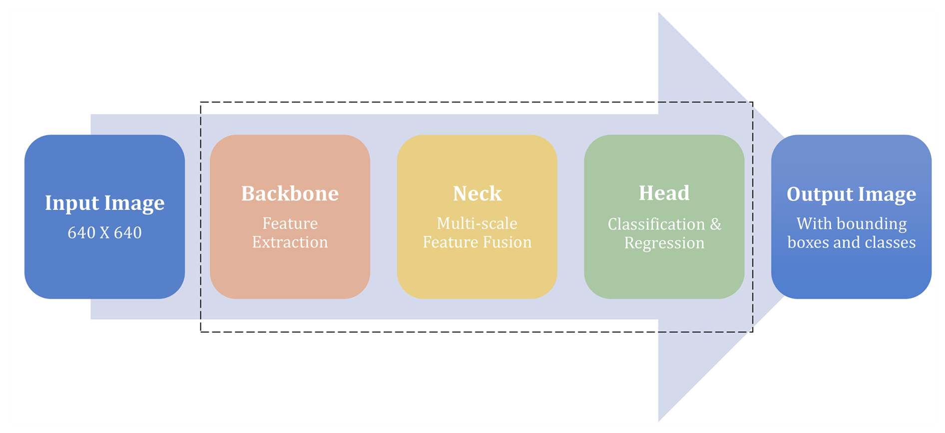
Figure 2 illustrates the high-level overview of the YOLOv8 architecture, consisting mainly of 3 components: a backbone network for feature extraction, a neck component for feature fusion, and a head component for final predictions (Ma et al., 2025). This streamlined architecture allows efficient single-shot object detection, completing the entire detection process in one forward pass. The Backbone helps in feature extraction. It has a series of convolutional layers, which are mathematical operations that scan the image using small filters to detect local patterns such as edges, textures, and shapes. The Neck acts as a bridge between the backbone and the head. It implements feature fusion that combines information from different scales. It uses both top-down and bottom-up pathways to combine high-level features with low-level spatial details. This ensures that final feature representations contain both the high-level understanding needed for accurate classification and spatial precision required for precise localisation. The Head represents the final prediction stage. It utilises two specialised networks, one focused solely on identifying what type of object it found, while the other focuses solely on determining the exact location.

3.2 Implementation workflow

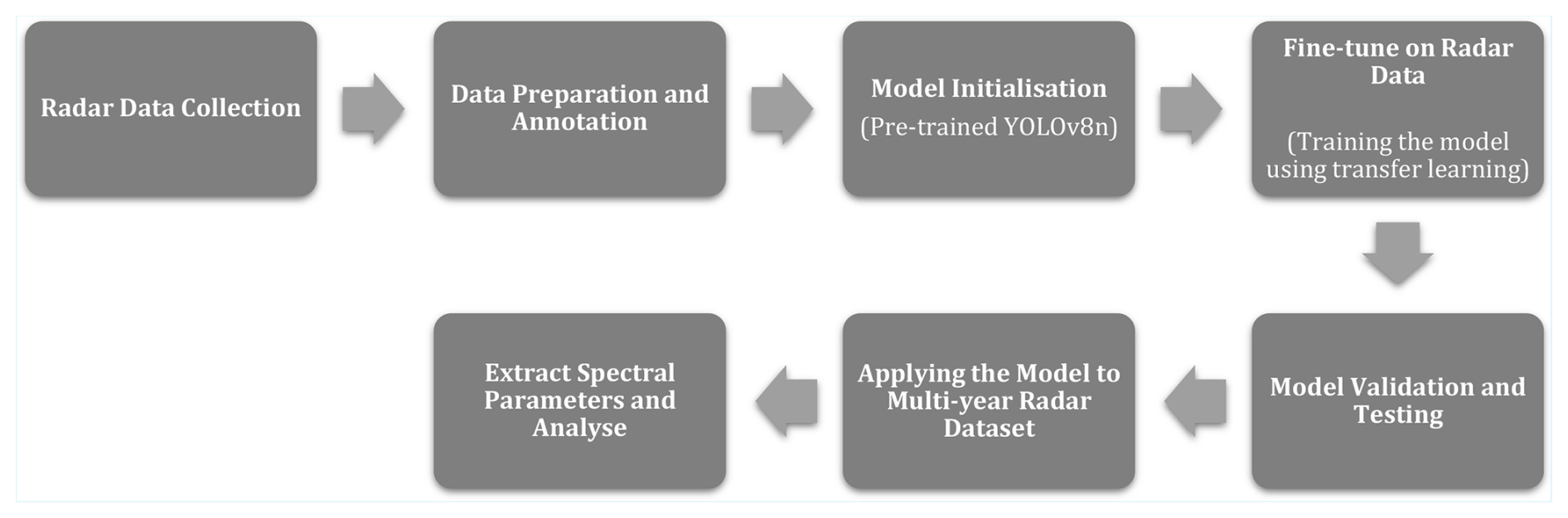
Figure 3 presents the detection methodology. The observational radar data were collected using the Saura radar. Each of these images in the dataset was annotated to label two different classes namely: “Target_Signal” and “Void”. Employing a transfer learning approach, the pre-trained YOLOv8n model was fine-tuned using the annotated radar spectra. Subsequently, the model was assessed using precision, recall, and mAP metrics (see Sect. 3.5). Once validated, the model was applied to detect LIME from the multi-year dataset. Detection's bounding box coordinates were converted to physical parameters. Each of these detections was then analysed to extract key parameters such as minimum altitude, maximum altitude, minimum frequency, and maximum frequency. Finally, these extracted data were analysed to understand the statistical behaviour of LIME.

3.3 Dataset preparation and annotation

For model training, testing, and validation, 200 images of radar spectra were selected based on manual inspection, prioritising clear examples of presence of distinct LIME. Each image in the dataset corresponds to one radar observation with a runtime of 220 s. Annotation tools were required to manually annotate these LIME signatures. For this purpose, we selected Roboflow (https://roboflow.com, last access: 3 October 2025) as the annotation platform for its user-friendly web-based interface and seamless export to YOLOv8 format, after evaluating alternatives such as the Computer Vision Annotation Tool (CVAT). The annotation process focused on identifying the LIME occurring at approximately 60 km altitude while ensuring clear separation from other echoes.

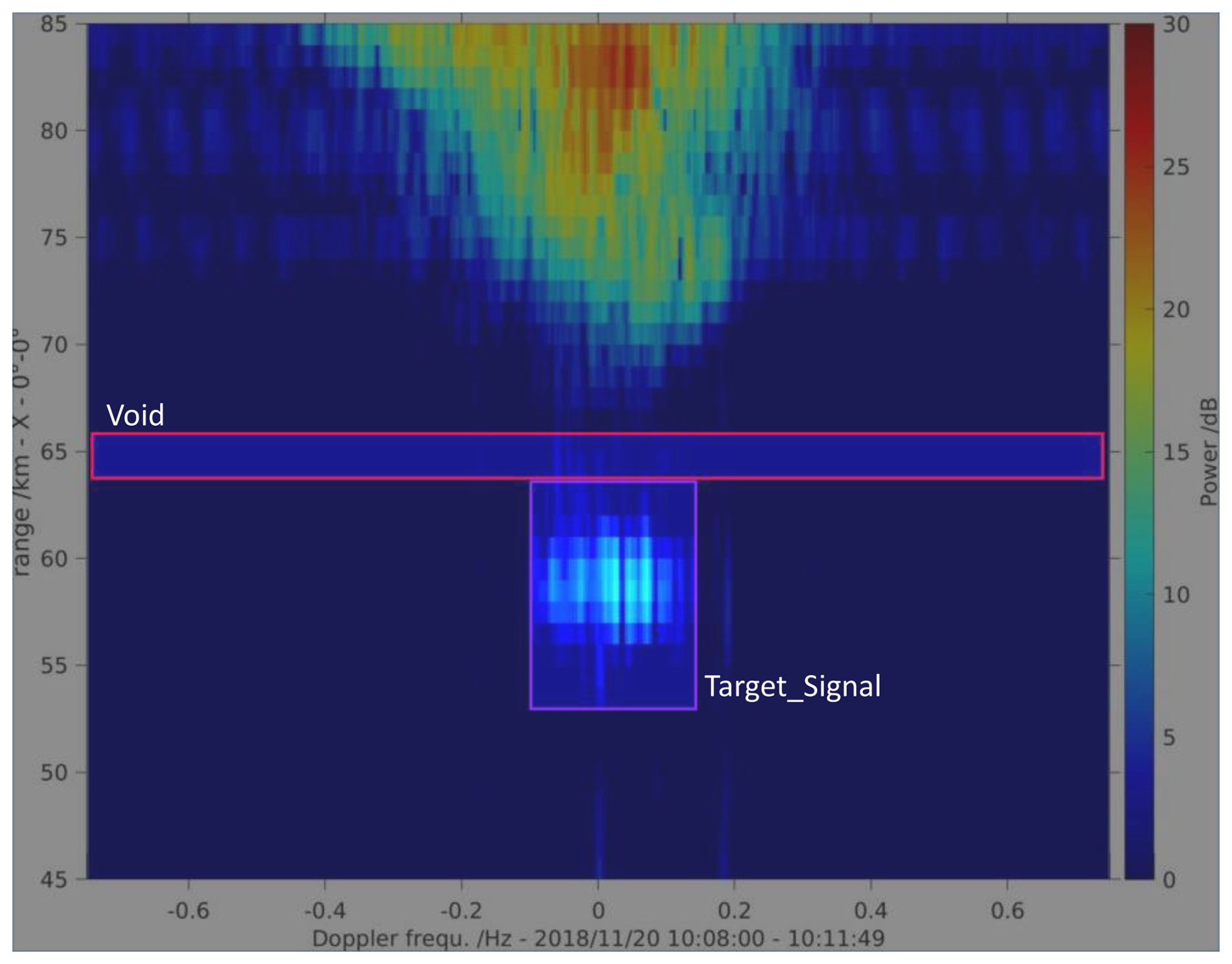
Figure 4 Example radar power spectrum showing annotated “Target_Signal” and “Void” classes used for YOLOv8 training, as displayed in the Roboflow annotation interface.

As illustrated in Fig. 4, for the annotation we employed a two-class system to address the specific challenge of correctly identifying LIME from the other echoes. LIME as defined earlier are isolated radar echoes appearing at an approximate altitude of 60 km with sufficient spatial separation from D region echoes that appear at higher altitudes. To ensure such spatial separation, the area with no signal presence directly above LIME was annotated as “Void” class, while the LIME signatures were labeled as “Target_Signal” class. The final dataset consisted of 200 radar spectra (PNG format). The dataset was further divided into 140 training images (70 %), 40 validation images (20 %), and 20 test images (10 %). After the completion of annotation, the dataset was exported from Roboflow in YOLOv8 format.

Table 1 Training configuration parameters. The optimizer refers to the algorithm used to update the model parameters during training to minimise prediction errors. The learning rate defines the step size of these updates. The batch size defines the number of training images processed simultaneously before the model parameters are updated.

Table 2 Pixel-to-physical unit conversion parameters.

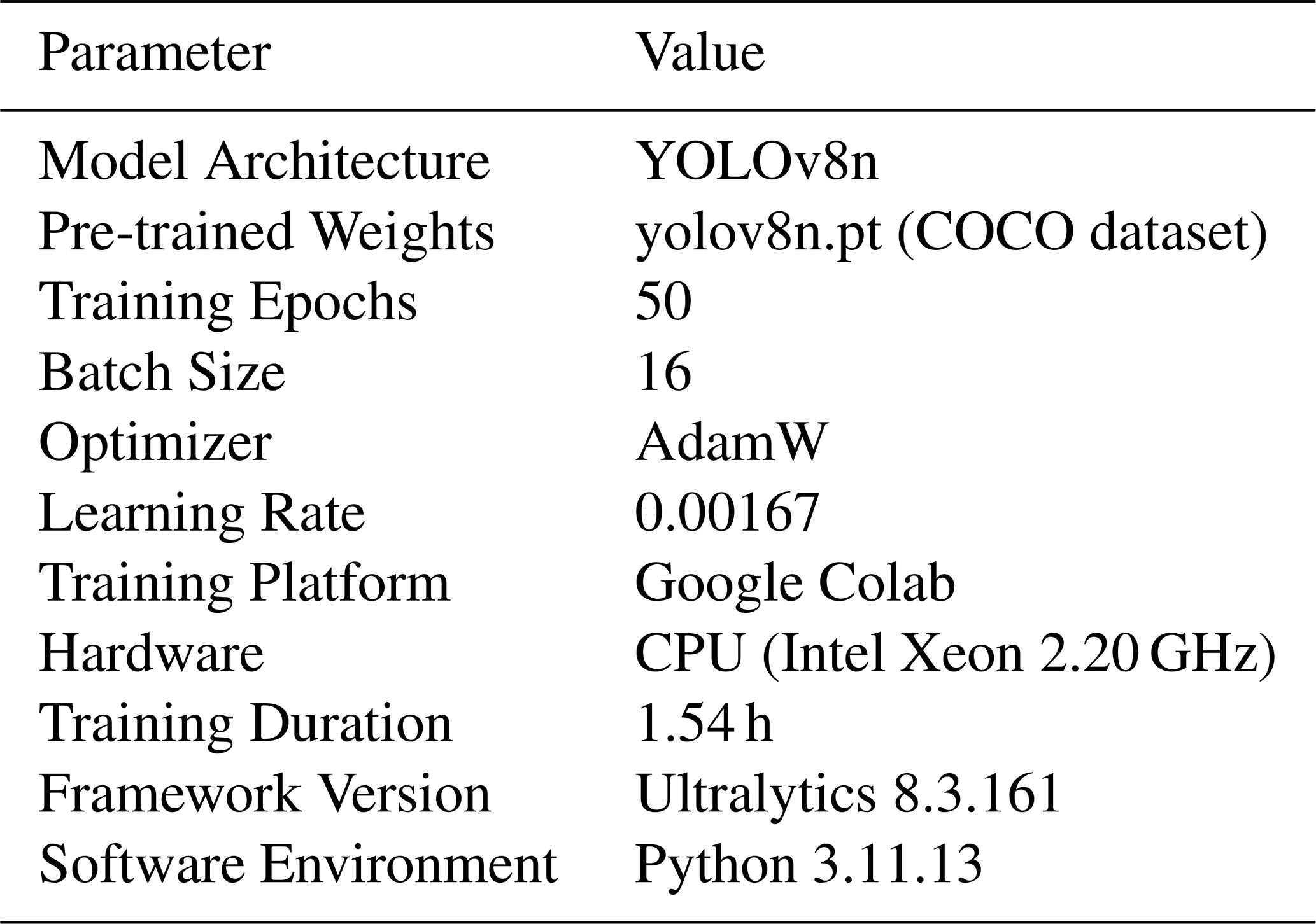
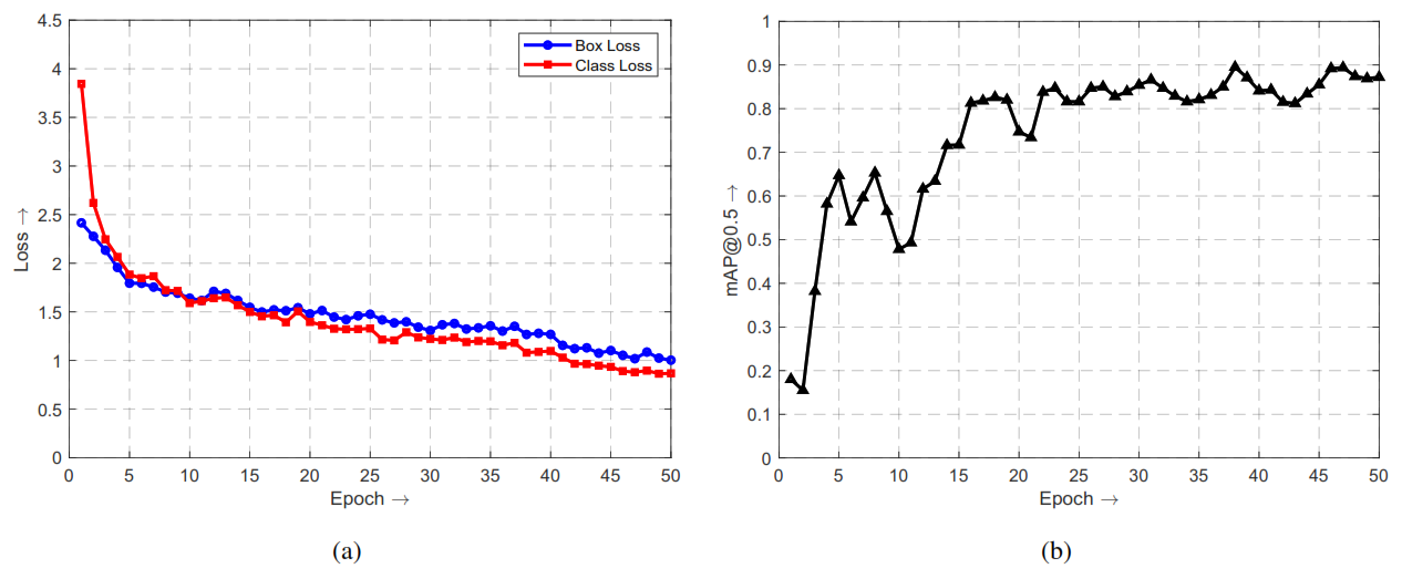
Figure 5 YOLOv8 training performance: (a) loss curves showing box loss and class loss; (b) mAP@0.5 evolution over training epochs.

3.4 Training configuration

In this work, we used Google Colab as the training environment. We employed transfer learning approach using a pre-trained YOLOv8n model, which was originally trained on the COCO (Common Objects in Context) dataset. The COCO dataset contains over 330 000 very diverse natural images with different shapes and sizes. These base models can be used as a starting point to adapt to a new task with limited datasets and less time (Ferguson et al., 2018). Pre-trained models have already learned the ability to extract detailed features like edges, textures, and colors. This feature extraction capability often remains applicable to new domains (Situ et al., 2023). The YOLOv8n base model was then fine-tuned by training it with the annotated radar spectra images for detecting LIME. This transfer learning approach eliminated the need to train the model from scratch and also allowed us to have a limited dataset of 200 annotated images. Data augmentation was applied using YOLOv8's default augmentation pipeline (Ultralytics, 2023).

The model was trained for 50 epochs, where one epoch represents a single complete pass of the training dataset through the model. Validation was performed after each epoch to monitor model convergence. Table 1 summarises the key training configuration parameters used in this work.

3.5 Performance metrics

For the purpose of evaluating the model, we used the standard object detection evaluation metrics (precision, recall, mAP50, and F₁). Precision, recall, and F₁ are defined by Eq. (1). Precision and recall values are derived from confusion matrix, which is a tabular summary of model predictions categorised into true positives (TP) that represent correctly detected LIME signature, false positives (FP) indicating wrong detections, and false negatives (FN) which denote missed LIME signatures. Precision measures the accuracy of positive predictions. Recall assesses detection completeness by determining the fraction of actual LIME successfully identified. The F₁ score provides a balanced measure of a model's ability to accurately identify LIME combining both precision and recall. These evaluation metrics have been widely adopted for assessing deep learning models in computer vision applications (Dev et al., 2017; Guo et al., 2024).

$$\begin{array}{}\text{(1)}& \begin{array}{rl}& \text{Precision}={\displaystyle \frac{\text{TP}}{\text{TP}+\text{FP}}}\\ & \text{Recall}={\displaystyle \frac{\text{TP}}{\text{TP}+\text{FN}}}\\ & F_{\mathrm{1}}={\displaystyle \frac{\mathrm{2}\times \text{Precision}\times \text{Recall}}{\text{Precision}+\text{Recall}}}\end{array}\end{array}$$

3.6 Automated detection pipeline

Following the model evaluation, the trained model was applied to multi-year (2018–2020 and 2024) radar datasets to detect LIME and extract altitude and frequency parameters related to LIME. Each of these yearly datasets contains between 84 000 to 92 000 radar spectra images.

Each yearly dataset was processed sequentially. A crucial part of the detection process was the two-class validation approach for confirming LIME isolation. The algorithm extracted parameters from the identified LIME only when both “Target_Signal” and “Void” classes were detected, with “Void” positioned above “Target_Signal”. This ensured that the detected echo represented LIME with sufficient altitude separation from D region echoes. It took approximately 3 h to process each year of spectra.

After detection, the algorithm calculated four key parameters through pixel-to-physical unit conversion: minimum altitude, maximum altitude, minimum frequency, and maximum frequency. The minimum altitude represents the lower boundary of the bounding box, while the maximum altitude represents the upper boundary of the bounding box. Similarly, the minimum frequency corresponds to the left boundary and maximum frequency corresponds to the right boundary of the bounding box. The pixel-to-physical unit conversion factors were defined by identifying the pixel boundaries of the radar spectrum plotting area and their corresponding physical measurement values, as specified in Table 2.

Table 3 Performance metrics overview.

Using the values from Table 2, altitude resolution (r_alt) and frequency resolution (r_freq) can be calculated as follows:

$$\begin{array}{}\text{(2)}& {\displaystyle }& {\displaystyle }{r}_{\text{alt}}={\displaystyle \frac{\mathrm{85}-\mathrm{45}}{y_{\text{bottom}}-y_{\text{top}}}}={\displaystyle \frac{\mathrm{40}\text{ km}}{\mathrm{548}\text{ pixels}}}\approx \mathrm{0.073}\text{ km per pixel}\text{(3)}& {\displaystyle }& {\displaystyle }{r}_{\text{freq}}={\displaystyle \frac{\mathrm{0.75}-(-\mathrm{0.75})}{x_{\text{right}}-x_{\text{left}}}}={\displaystyle \frac{\mathrm{1.5}\text{ Hz}}{\mathrm{655}\text{ pixels}}}\approx \mathrm{0.0023}\text{ Hz per pixel}\end{array}$$

Given the bounding box $\mathit{X}=[x_{\text{min}},y_{\text{min}},x_{\text{max}},y_{\text{max}}]$ predicted by the model for a detected LIME, where (x_min,y_min) and (x_max,y_max) represent the top-left and bottom-right pixel coordinates respectively. Physical parameters where then calculated as:

$$\begin{array}{}\text{(4)}& \begin{array}{rl}& h_{\text{min}}=\mathrm{85}-(y_{\text{max}}-y_{\text{top}})\times r_{\text{alt}}\\ & h_{\text{max}}=\mathrm{85}-(y_{\text{min}}-y_{\text{top}})\times r_{\text{alt}}\\ & f_{\text{min}}=-\mathrm{0.75}+(x_{\text{min}}-x_{\text{left}})\times r_{\text{freq}}\\ & f_{\text{max}}=-\mathrm{0.75}+(x_{\text{max}}-x_{\text{left}})\times r_{\text{freq}}\end{array}\end{array}$$

where h_min and h_max represent the minimum and maximum altitudes in km, and f_min and f_max represent the minimum and maximum frequencies in Hz.

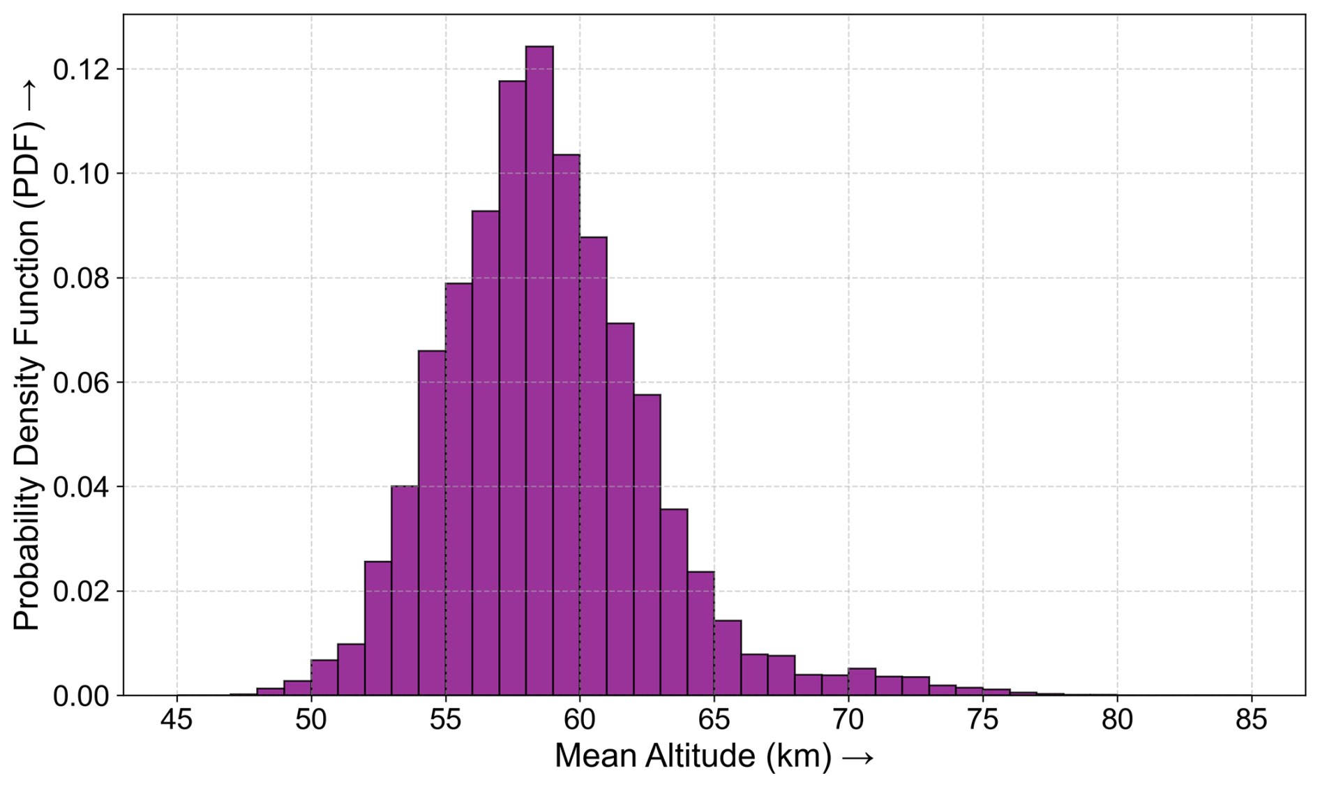
Figure 6 Probability density function (PDF) of mean altitudes for all valid LIME detections from 2018–2020 and 2024 (12 677 total valid detections).

4 Results

4.1 Model performance

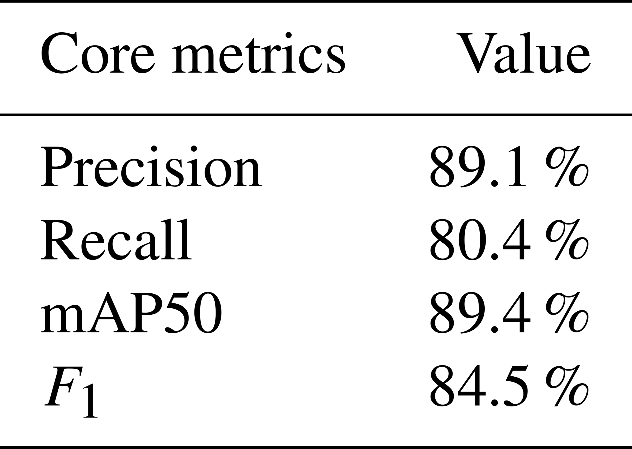
Model performance was evaluated on the validation set consisting of 40 annotated radar spectra. Core performance metrics are presented in Table 3.

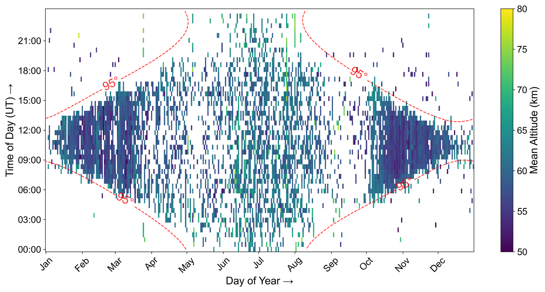
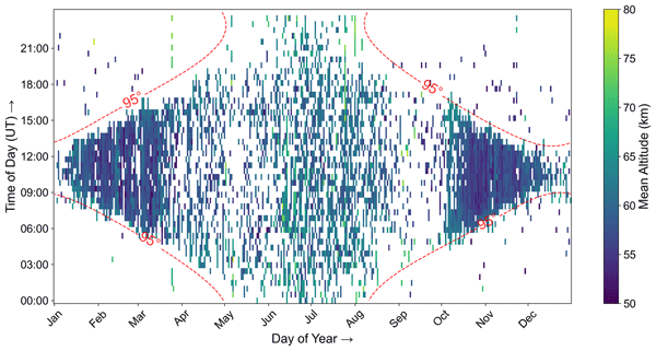
Figure 7 Altitude distribution of LIME detections from years 2018–2020 and 2024. Data binned by day of year and 30 min time intervals, with colors representing mean altitude averaged across all years for each day-time bin. The red dashed contour marks the solar zenith angle of 95°, calculated at ground level at the radar location, used here as an approximate indicator of the daylight conditions at the altitudes of interest.

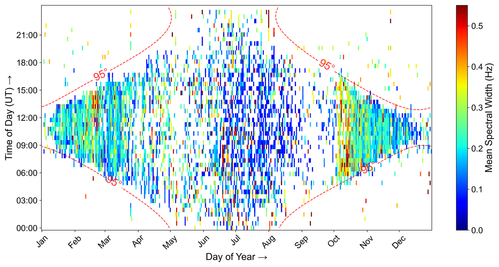
Figure 8 Detection box spectral width distribution of LIME detections from years 2018–2020 and 2024. Data binned by day of year and 30 min time intervals, with colors representing mean spectral width averaged across all years for each day-time bin. The red dashed contour marks the solar zenith angle of 95°, calculated at ground level at the radar location, used here as an approximate indicator of the daylight conditions at the altitudes of interest.

The trained model achieved 89.4 % mAP50, with precision (89.1 %) notably higher than recall (80.4 %). The higher precision compared to recall indicates fewer false positives than false negatives. The overall F₁ score of 84.5 % demonstrates robust detection performance.

YOLOv8 training optimises two loss components, where loss refers to a numerical measure of how far the model's predictions are from the correct answers, with a lower loss indicating better performance. Box loss measures the error in predicted bounding box localisation, while class loss measures the error in distinguishing between “Target_Signal” and “Void” classes. Training losses over 50 epochs are illustrated in Fig. 5a. Both losses exhibited rapid initial decrease during the first 10 epochs, followed by progressively smaller improvements in later epochs. The consistent downward trend without significant oscillation demonstrates effective model optimisation. Figure 5b illustrates the mAP50 evolution during training. The mAP50 exhibited rapid improvement during the initial 15 epochs, increasing from approximately 0.18 to 0.80. Performance continued to improve gradually, stabilising around 0.85–0.90 after epoch 20.

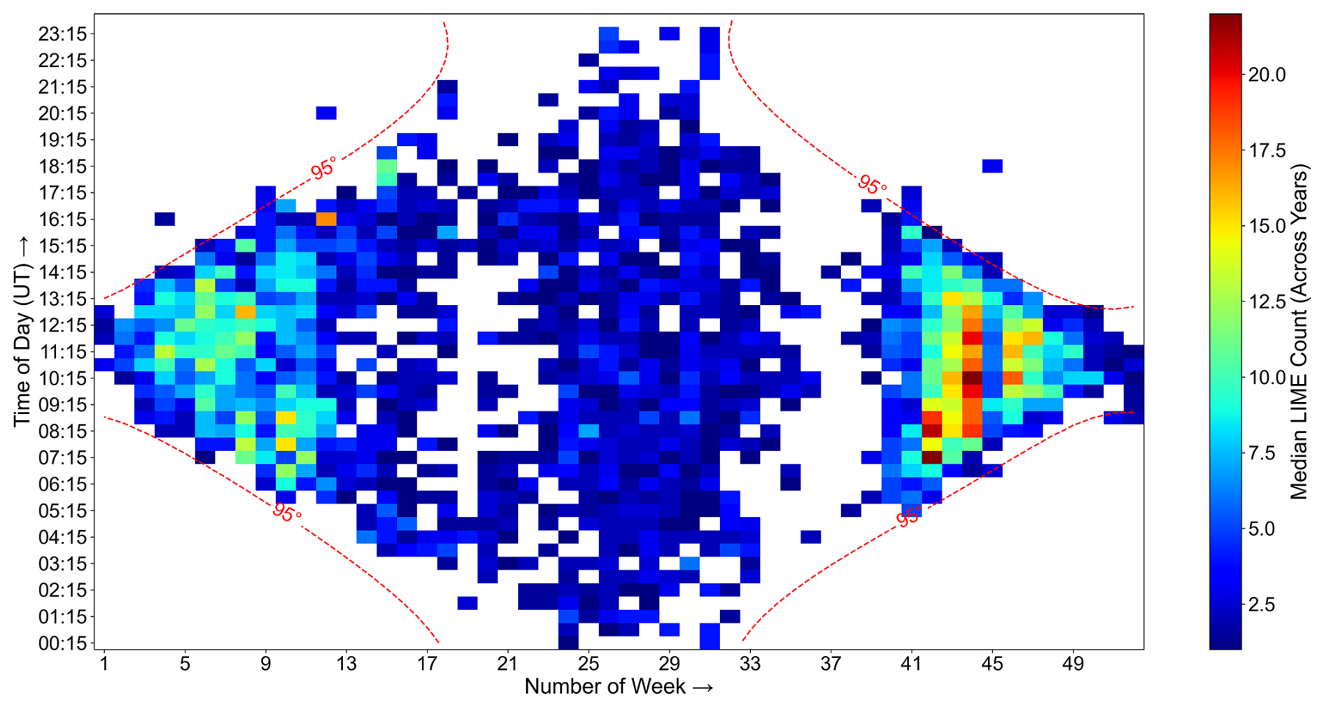
Figure 9 Weekly temporal distribution of median LIME occurrence from years 2018–2020 and 2024. For each week–time bin, the median occurrence is calculated across the four years. The red dashed contour marks the solar zenith angle of 95°, calculated at ground level at the radar location, used here as an approximate indicator of the daylight conditions at the altitudes of interest.

4.2 LIME characteristics

Physical parameters (altitude and frequency bounds) were extracted from each detection following the methodology described in Sect. 3.6. The mean altitude for each LIME detection is calculated as the average of the minimum and maximum altitude bounds of the bounding box. Spectral width is the difference between maximum and minimum frequency bounds. The automated pipeline processed radar spectra across four years (2018–2020 and 2024), identifying 12 677 LIME signatures that satisfied the two-class validation criterion. The following subsections present statistical analysis of the extracted parameters from the detected LIME.

Figure 10 Daily LIME duration distributions from years 2018–2020 and 2024.

4.2.1 Mean altitude distribution

The composite mean altitude distribution from 12 677 valid detections across 2018–2020 and 2024 is shown in Fig. 6. The distribution exhibited a primarily Gaussian profile with mean altitude of 58.8 km and median of 58.5 km, with a standard deviation of 3.9 km, indicating the predominant occurrence of LIME just below 60 km altitude. The detections above 70 km appear to be outliers, which can be faint EPP-related echoes without substantial absorption above, aircraft reflections or possibly also caused by interference. Figure 7 shows the composite temporal-altitude heatmap of LIME detections from all observational years as a function of day of year and time of day, with colors indicating the detected mean altitude. The red dashed contour marks the solar zenith angle of 95°, calculated at ground level at the radar location, used here as an approximate indicator of the daylight conditions at the altitudes of interest. The vast majority of detections (99 %) occurred when the solar zenith angle remained below 95°, indicating the necessity of solar illumination for the generation of LIME. A seasonal variation in the altitude can be observed, with LIME appearing at a higher altitude during summer months (April to September) compared to winter months. For the majority of LIME cases, we found a total layer thickness (uppermost minus lowermost detected range) of 6 to 10 km, while the largest values originate from events formed by two adjacent layers.

4.2.2 Spectral width analysis

Figure 8 shows the composite temporal-spectral width heatmap of LIME detections from all observational years as a function of day of year and time of day, with colors indicating mean spectral width. Note, the shown spectral widths do not represent fitted widths of the individual range-resolved echoes, but the width of the YOLO detection box (see e.g. Fig. 4). With that, they will tend to overestimate the spectral widths of the echoes. The heatmap indicates substantial variability in the spectral width of the LIME throughout the year. Seasonal variation was evident with October-March detections showing broader spectral widths (median = 0.21 Hz) compared to April–September (median = 0.14 Hz), indicating approximately 50 % seasonal increase.

4.2.3 Temporal patterns

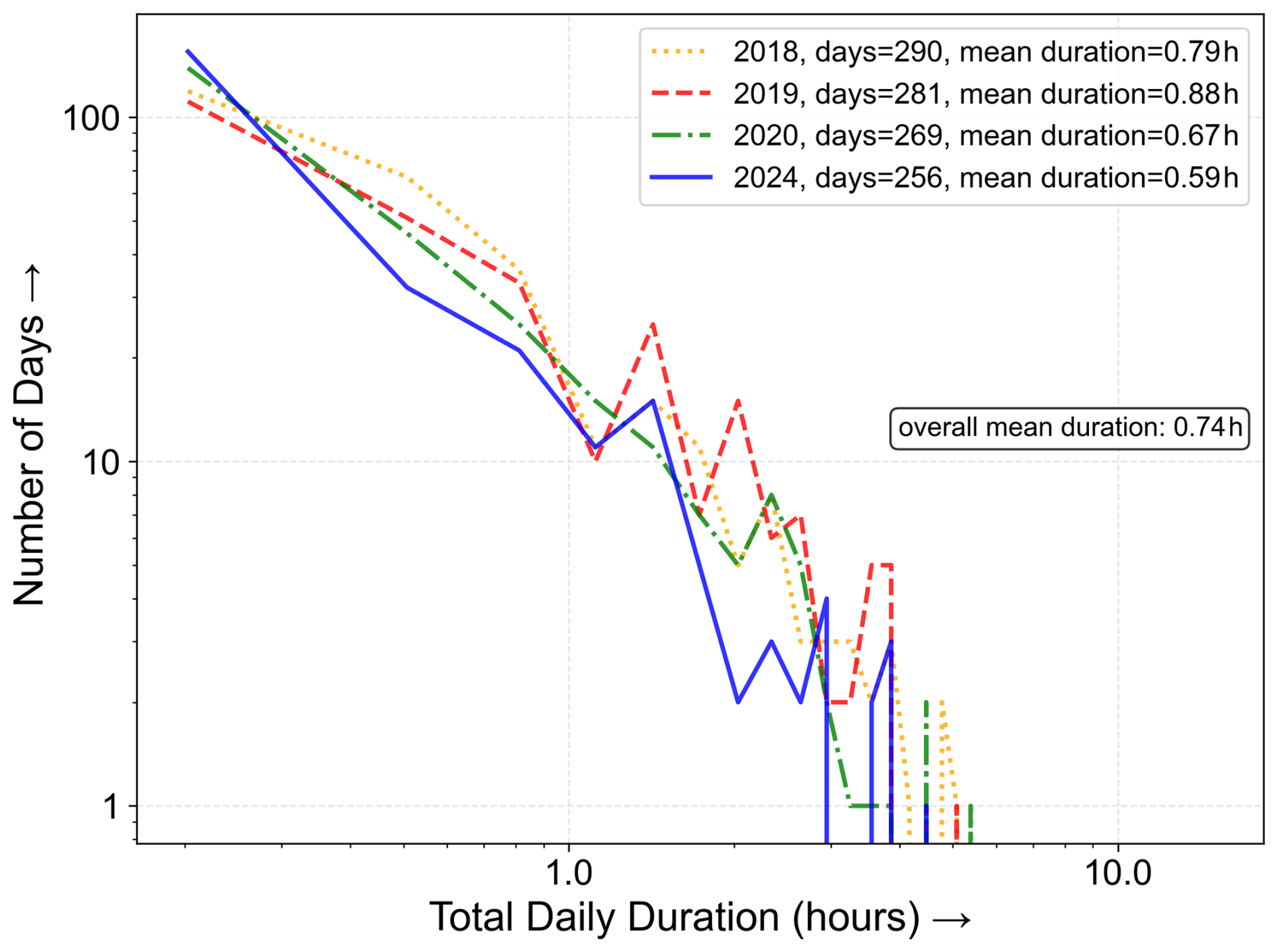
Figure 9 displays the median number of LIME detections per 30 min time bin for each week of the year, computed across four years of observations (2018–2020 and 2024). For each week and time bin combination, the median is taken across the four yearly values, making it more robust against outliers compared to the mean. The maximum observed median value is 22 detections per 30 min bin. The heatmap indicates that LIME appear more frequently during the winter weeks than during summer weeks. In summer, LIME were detected almost throughout the entire day due to low solar zenith angle (SZA), but the overall occurrence count remained low compared to winter weeks. Figure 10 shows daily signal duration distribution for all observational years, calculated as the number of detections per day multiplied by the individual radar experiment duration. The distribution exhibited exponential decay, with most days showing durations below 1 h. Mean daily durations varied across years, ranging from 0.59 h (2024) to 0.88 h (2019), with an overall mean duration of 0.74 h.

5 Discussion

5.1 Discussion of previous findings

As we initially pointed out, radar echoes from an altitude of around 60 km are not uncommon at polar latitudes due to the presence of EPP (Hall et al., 2006). They can actually be observed for up to 40 % of the time, but the majority of detected events were at 65 km altitude (Renkwitz and Latteck, 2017). Note, these EPP-related radar echoes can be identified by their typical annual occurrence with a clear preference around the equinoxes as well as very distinct characteristics in the spectra of the radar time series. EPP events considerably enhance the ionisation of the lower D region for areas with an extent of several dozens of km. Depending on the involved energies of EPP virtual radar layers at e.g. 60 km are formed. As the radiation pattern of the Saura PR is imperfect, sidelobe contributions are evident. As an example, for 30 km (60 km) horizontal displacement from the radar, the oblique echoes from 60 km altitude will be observed at 67 km (85 km) range. For multiple points, pronounced parabolic arcs appear in the range intensity image spectra (see Fig. 11b) as the radial velocity component of the oblique echoes will be dominated by the horizontal winds.

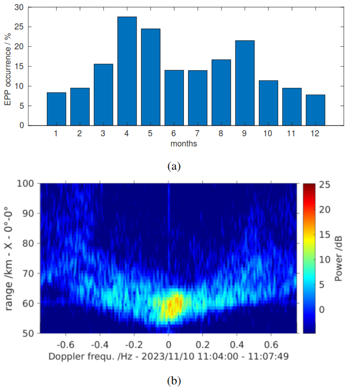
Figure 11 (a) Monthly mean occurrence rate of EPP in the mesosphere, detected by the Saura radar for the years 2003–2023. (b) Image power spectrum of Saura for one experiment on 10 November 2023 displaying clear Doppler- and range-spread EPP signatures with a bottom altitude of about 56 km.

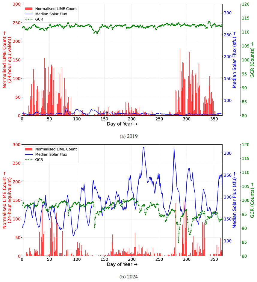
Figure 12 Comparison of normalised LIME counts, median solar flux, and galactic cosmic ray counts for (a) 2019 and (b) 2024, a solar minimum and maximum year, respectively. LIME counts are normalised by daylight hours (SZA ≤ 95°).

For the majority of such strong EPP, reaching 60 km altitude, the radar wave's energy is strongly absorbed above that altitude, resulting in the absence of any radar echoes in the upper D region and above (note the absence of echoes near 0 Hz above 70 km in Fig. 11b). In the case of LIME, no evidence of parabolic shaped signatures in the image spectra was found (Fig. 1b), nor is it clearly discernible in the statistics of the detection boxes spectral widths (see Fig. 8). Nevertheless there were situations when EPP-related echoes were observed at higher altitudes, e.g. near 70 km, and LIME occurred near 60 km, which, however, still did not show any EPP-like image spectrum.

The LIMEs statistically have an obviously different occurrence distribution (Fig. 9) than EPP-related radar echoes (see Fig. 11a, similarly to Fig. 9 in Renkwitz and Latteck (2017), but extended to the end of 2023). LIME and EPP also show a clearly different altitude distribution. For LIME the winter season, October to March, seems to be preferred, which is possibly supported by the absence of the typical lower D region echoes as the solar zenith angle is too large. During summer, when the smaller solar zenith angle allows a lowered bottom side of the D region, LIME might be masked by the typical echoes. However, we might still expect to observe enhanced signatures of them at sunrise when the D region is yet not fully formed and equivalently for the sunset, which is not obvious in the shown statistics. At this point, we may only speculate, that the generation mechanism allowing LIME is reduced during the summer months.

We also investigated a possible relation between the appearance of LIME and solar activity. The normalised echo detections are depicted with the solar flux in Fig. 12a and b for the two years 2019 and 2024, which represent solar minimum and maximum conditions. We also depict the galactic cosmic rays (GCR) detection rate obtained from the Oulu Neutron Monitor station, Finland, via the NMDB database (NMDB, 2026) for the individual years. For 2024 a quite prominent reduction in GCR is visible for solar active periods. EPP events are preferably seen during the ascending and descending phase of the solar maximum. Obviously LIME have been observed less frequently during solar maximum years. We found weak correlation for solar minimum years between the LIME occurrence and the solar flux ($r=-\mathrm{0.27}$ for 2019), whereas no correlation was found for the solar maximum year ($r=-\mathrm{0.08}$ for 2024).

Interestingly, there are enhanced spectral widths visible for consecutive days in February and October for the four year average in Fig. 8. Spectral widening can be interpreted as enhanced turbulence, which might be caused by various dynamical situations like e.g. shear winds. However, the prominent intensification is quite remarkable and a possible source like changes in tidal activity at these altitudes needs to be investigated in future studies.

Also, the detected altitudes seem to have preferred seasons (Fig. 7), where during October to March altitudes around 57 km are seen, whereas during summer higher altitudes are observed (≈ 61 km). This change of altitude occurs simultaneously with the reduction of spectral width and both could be an indicator for changes in the underlying driving mechanism of LIME.

The reduced occurrence of the echoes during summer is also visible in Fig. 10, where the long lasting echoes are comparably rare despite the long sunlit period during these months. Shorter durations up to one hour are much more frequently occurring during the short sunlit winter period.

Concerning possible false detections, we manually inspected some isolated detections that were associated with enhanced Doppler shift and spectral width. These short-lived detections are believed to originate from aircraft flying at a distance of about 55 km east of the radar, based on their appearance. These false detections were later suppressed by filtering the detected radar echoes Doppler shifts.

The detections outside the sunlit period are possibly caused by weak and rather local EPP events that don't show intense absorption above the precipitation altitude, or by interference from other transmitters, but at most they only represent 1 % of the total detections. We are therefore confident to have established a robust detection of LIME using YOLO.

5.2 Discussion of related/comparative studies

The example that gets closest to our observations of LIME are shown in Fig. 10 of Reid (2015) for the other large aperture PR radar at Buckland Park, Australia. It was taken at local morning hours (06:35 LT), when the D region was not yet fully developed. The prominent structure at 62 km range resembles what we observed and described as LIME. The duration of the event and continued visibility of the D region agrees to our findings. This observation at middle latitudes also demonstrates, that the underlying process is not a polar phenomenon.

A corresponding report about radar echoes that seemed to occur from below the D region was given by Rasmussen et al. (1980) using a bi-static ionospheric VLF/LF sounder. For the rather distant bi-static measurements they deduced the reflecting altitude at around 66 km with a thickness of 6 km and interpreted it as a layer of constant conductivity. Equivalent experiments in Brazil conducted in 1980 have shown similar results (Klemetti et al., 1988). Bain and Kossey (1987) addressed the initial publication by Rasmussen et al. (1980) and numerically found suitable altitudes near 63 km.

Even though the mentioned altitudes are near to what we report here, we are not certain if it's the same phenomenon as their plots show consistent echoes for consecutive days including the night times. Furthermore, the much lower frequency used in their experiments means that also much smaller electron densities were required, and one could also question the appropriate electron density profile they assumed for the reflection height calculations.

Bertoni et al. (2013) associated VLF observations to the C region, which noteworthily coincide in altitude and local time with the example by Reid (2015). The authors refer to earlier measurements of electron density by rocket soundings that have shown enhancements just above 60 km altitude (Mechtly et al., 1967; Mechtly and Smith, 1968).

Another report on low altitude ionospheric echoes is given by Rietveld et al. (1996) using the EISCAT heater near 4 MHz frequency. For the experiments conducted around local noon, signatures from below 60 km are prominent in their Fig. 7. Noteworthy, the electron density profile depicted in their Fig. 9 seems to resemble a rather enhanced ionisation state with 1e10 electrons m⁻³ at 80 km altitude. Together with the comparably weak higher altitude D region echoes this scenario might rather be EPP related.

Later experiments by Vierinen et al. (2013) with the same heater conducted on seven days in December 2011 for 1.5 to 4 h duration during noontime have again shown radar echoes from 60 km altitude and partly below. During these days no significant geomagnetic disturbance was found, nor did we see any EPP spectra in Saura radar data (130 km distant to the EISCAT heater). Therefore, it is very likely no EPP occured during these days that could have additionally ionised these low altitudes. Furthermore, in the examples shown, no clear separation between the ordinary D region echoes and the 60 km echoes is visible, which may represent a rather typical and consistent electron density profile. Considering the amount of radiated power involved in these heating experiments, regular detection of echoes from as low as 60 km altitude with a radar frequency of 4 to 5 MHz seems plausible, but we are uncertain if these detections are related to the LIME we investigate in this manuscript.

5.3 Discussion on the cause of the phenomenon

As in most cases the observed LIME have a rather faint intensity, which indicates comparably small gradients in the radar refractive index, which is defined by the electron density profile. Possible speculations for the appearance of LIME are:

• The present turbulence forms structures of explicitly favourable sizes in the refractive index under a nominal ionisation scenario. If so, why does this show altitude changes during sunrise and sunset whereas they remain static most of the time in between at specific altitudes?

• Favourable conditions of mesospheric wind dynamics, resulting in a compression and accumulation of more neutrals like nitric oxide that are then ionised by the same nominal ionisation source?

• May changes of the incident ionisation source cause the visibility at preferred heights?

One possible ionisation source, galactic cosmic rays, may easily reach lower atmospheric altitudes, and are measured on or above the ground, e.g. by stratospheric balloons. GCRs are also reported to contribute as an ionisation source for the lowermost part of the D region (Nicolet and Aikin, 1960; Abdu et al., 1973). Interestingly GCRs should be reduced during enhanced solar activity and specifically during solar coronal mass ejections (CME), which is called Forbush decrease (see e.g. Ross and Chaplin, 2019; Sierra-Porta, 2024; Riggi et al., 2025). From the last solar minimum to the current solar maximum GCR reductions of 30 % and more have been observed. With the enhanced solar activity during 2024 and thus a reduction in GCR, we may also expect a reduced occurrence of LIME. This can actually be seen comparing Fig. 12a and b, which suggests GCR may serve as a significant ionisation source for altitudes just below 60 km during solar minimum years. The contribution of GCR would also represent a clear difference to the primarily Lyman-alpha controlled quiet D region.

5.4 Discussion about YOLO

Having discussed LIME characteristics from different perspectives like seasonal dependencies, solar flux correlations, and comparative analyses with the existing literature, we now discuss the methodological framework used for this study. The YOLOv8 object detection framework demonstrated robust transfer learning from natural images to atmospheric radar spectra images, achieving 89.4 % mAP50 with only 200 annotated images. As noted in the Introduction, YOLO's demonstrated generalisation capability to specialised domains make it well-suited for the application to detect LIME, with recent studies confirming similar success across other remote sensing applications (Ma et al., 2025). The higher precision (89 %) than recall (80.4 %) indicates that the model favours reducing false positives at the expense of missing some true LIME detections. The automated detection approach processed one year of radar spectra in approximately 3 h. This allowed systematic multi-year analysis that would have taken a substantially longer time with manual inspection. Future work could focus on improving the detection performance of the YOLOv8 model through improved annotation strategies and systematic hyperparameter tuning, potentially increasing the mAP50 beyond the current 89.4 %.

6 Conclusions

In this study, we present the systematic analysis of radar echoes occurring from altitudes often below 60 km, which are clearly separated in altitude from the regular D region. From this general appearance we named these radar echoes Low-altitude Isolated Mesospheric radar Echoes (LIME). These echoes were occasionally seen in typical radar range-time-intensity plots, but manual inspection for statistical analysis turned out to be very tedious and prone to human errors. Therefore, the deep learning approach analysing about 350 000 image power spectra for four years of radar observations revealed it as a still quite frequent phenomenon. The fine-tuned YOLOv8 model achieved 89.4 % mAP50 (mean Average Precision at an Intersection over Union threshold of 0.50, where higher values indicate better detection performance) with only 200 annotated spectra.

So far, the only other prominent example of a LIME detection was presented by Reid (2015). The reason for that is likely given by the required radiated power, sensitivity and beam width of the vertically sounding MF/HF radars. Many LIME are actually rather faint echoes and will likely not be seen by compact MF/HF radars used for the explorations of dynamics in the mesosphere and lower thermosphere.

The application of YOLO provided a robust and efficient way to detect and study these rarely described radar echoes from the lower mesosphere. Thus, this analysis provided new insights into the occurrence of LIME.

The echoes are a daytime phenomenon, they exclusively occur during the sunlit period (99 % for solar zenith angle <95°). The winter season (October to March) is the preferred period, during which the echoes also show enhanced spectral widths for a few consecutive days. Whereas during summer, LIME seem to occur less frequently and with smaller spectral width. The preferred altitudes are near 57.5 km ± 4 km, whereas during summer the echoes are seen near 62 km. The observed layers show a typical total altitudinal width of 6 km, whereas double layers extend to 10 km. For the solar minimum years 2018–2020 a weak negative correlation between LIME and solar activity was found, which was absent for solar maximum year 2024. For the same solar maximum year, we found a substantial decrease in LIME detections. We attribute this decrease to the reduction in GCR flux caused by enhanced solar activity (Forbush decrease). Assuming this, we speculate that GCR might be responsible for LIME visibility and thus demonstrate to play a significant role for ionisation processes just below 60 km altitude.

In summary, the designation “C region/layer” phenomenon may be appropriate given the distinct altitudinal separation between LIME and the regular D region echoes and the potential contribution of GCR to the formation of a layer just below 60 km altitude.

Continued observations and an extension of the analysis to more years of existing data will improve the statistics, and may strengthen or clarify the speculated connection of GCR to the visibility of LIME. Furthermore, extending the investigations to multibeam data (off-vertical radar soundings) might indicate process properties like aspect-sensitivity or isotropy. A detailed analysis of the echoes spectral widths may also be a valuable indicator of turbulence intensity at these lower mesospheric altitudes. For this, we also plan to test a connection of LIME to dynamical processes, but this might widely depend on model data as observational wind data are sparse at these altitudes. Furthermore, it will be worth to investigate a possible difference between both magneto-ionic components, of which only the extraordinary mode was used in this study.