Impact of cloud seeding on simulated hailstorms and its dependence on CAPE, wind shear, and tracking thresholds

Hailstorms are a damaging weather phenomenon worldwide. In response, several countries – including Switzerland – have implemented hail mitigation strategies, most notably through cloud seeding with ice-nucleating particles (INPs). In this study, we investigate the impact of silver iodide (AgI) perturbations on eight convective storms observed in Switzerland and southern Germany. Our focus is on evaluating the effectiveness of an early seeding strategy and examining its relationship with two key meteorological parameters: Convective Available Potential Energy (CAPE) and 0–6 km wind shear. We also assess how different storm-tracking thresholds influence the interpretation of seeding effects. Simulations were conducted using the Consortium for Small-Scale Modeling Regional Weather and Climate Model (COSMO). AgI particles were introduced as a prognostic variable during the cumulus stage and released into the updraft region near the cloud base at a concentration of 20 cm⁻³. The results indicate that early seeding increases both the mass and number concentration of ice and graupel, accompanied by stronger updrafts. In contrast, the response of hail mass is ambiguous and varies with the tracking method. Hail size and hail-covered area also show no systematic dependence on CAPE or wind shear. Despite the variability in the hail response, our results show that early seeding increases the mean hail diameter in 80 % of the cases, with a median increase of 7.6 % – corresponding to a 31.3 % increase in kinetic energy – while simultaneously reducing the spatial extent of the hail-affected area by 39.8 % (median), with 92.4 % of simulations exhibiting a decrease in hail area.

1 Introduction

Hailstones produced by thunderstorms are a damaging weather phenomenon observed in many regions worldwide. In some locations, hail occurs on average more than once per year (Allen et al., 2020). In the United States, the average annual loss from severe convective storms is estimated at USD 11.23 billion (2016 USD), comparable to the USD 11.28 billion in losses from hurricanes (Gunturi and Tippett, 2017). Across Europe, severe hailstorms are also a major hazard, regularly causing substantial damage to buildings, crops, and vehicles, and resulting in significant economic and insured losses (Punge and Kunz, 2016). Switzerland is also vulnerable. For example, the extreme hailstorm on 21 June 2021 caused building damage amounting to CHF 400 million (approximately EUR 415 million) in a single canton alone (Kopp et al., 2023; Schmid et al., 2024). In Europe, the pre-Alpine regions north and south of the Alps are especially prone to hail (Nisi et al., 2016; Fluck et al., 2021; Feldmann et al., 2023), with occurrence showing strong year-to-year variability and a pronounced seasonal cycle (Schröer et al., 2023). Within Switzerland, certain areas such as southern Ticino, the Napf region, and the Jura stand out as hail hotspots (MeteoSwiss, 2025). In these regions, hail falls on average 2 to 4 d km⁻² each summer – rates that exceed those of most hail-prone areas in Europe.

Given the widespread damage hailstorms can cause across regions like Switzerland, understanding the atmospheric conditions that favor their development is essential. This concern motivates a closer examination of the environmental parameters that govern convective storm behavior. A growing body of observational and theoretical research supports the hypothesis that convective storm type is largely determined by a relatively small set of atmospheric variables (Weisman and Klemp, 1982). Among the most influential are CAPE and vertical wind shear, both of which play critical roles in storm evolution and structure. CAPE quantifies the energy available to an air parcel originating from a low atmospheric level and rising adiabatically; if the parcel becomes buoyant relative to its surroundings, it accelerates upward. For deep, moist convection to occur, two conditions must typically be met: the presence of CAPE and a sufficiently strong forcing mechanism to release it (Groenemeijer and van Delden, 2007). Interestingly, some convective storms have been documented in environments with little or no CAPE, as noted by Carbone (1982, 1983) and Forbes (1985). Vertical wind shear also strongly influences storm organization by inducing dynamic pressure perturbations (Markowski and Richardson, 2010). In weak shear environments, single or ordinary cells tend to form – typically short-lived and rarely severe (Byers and Braham, 1949). As shear increases, multicell storms become more likely, often producing severe weather and hail. Under strong shear conditions, supercells may develop, characterized by deep, persistent rotating updrafts (Doswell and Burgess, 1993) and the frequent production of large hail. A study by Groenemeijer and van Delden (2007) in the Netherlands shows that the likelihood of a sounding being associated with hail increases with higher values of both CAPE and shear. However, the typical large hail event is most commonly linked to shear in the 10–20 m s⁻¹ range, as environments featuring both high CAPE and strong shear are relatively rare.

Driven by the recurring and often costly impacts of hailstorms, Switzerland has invested in hail mitigation strategies – particularly in the pre-Alpine regions, where the frequency and severity of hail events are most pronounced. Among the most notable initiatives are the large-scale weather modification experiments Grossversuch III and Grossversuch IV. Grossversuch III, conducted from 1957 to 1963, was a randomized field experiment designed to test whether hail could be suppressed by releasing large quantities of silver iodide (AgI) smoke from ground-based generators. The experiment focused on the Canton Ticino and the adjoining Mesolcina Valley. While AgI seeding was sometimes found to substantially increase rainfall, the hail-suppression results were less conclusive (Schmid, 1967). Grossversuch IV was carried out in central Switzerland over five years (1977–1981), near the Napf/Entlebuch hail hotspot (MeteoSwiss, 2025), with participation from research groups in France, Italy, and Switzerland. The first evaluation of the Swiss Grossversuch IV experiment, which used AgI rockets following the Soviet method, reported no statistically significant differences between seeded and unseeded hail cells (Federer et al., 1986). However, a subsequent re-analysis of the same dataset reached the opposite conclusion, showing that seeding can increase hail kinetic energies in some cases (Auf der Maur and Germann, 2021). More recently, in 2018, Switzerland launched a new hail mitigation campaign in its northern region, timed to coincide with the country's hail season from May to September (Baloise Group, 2018). This initiative used a lightweight aircraft equipped with generators and pyrotechnic flares, which had been rigorously tested for effectiveness in laboratory conditions (Chen et al., 2024). The campaign adopted the updraft seeding method – first introduced in 1948 and now widely used in operational weather modification efforts worldwide (Foote and Knight, 1977) – targeting convective clouds during their cumulus stage and seeding from an aircraft that circles below the cloud base. The seeding material was silver iodide (AgI), a common and effective cloud-seeding agent (Marcolli et al., 2016; Chen et al., 2024), and served as the primary active substance in both flares and generators (Holleman and Wieringa, 2006).

All of these hail mitigation strategies are based on the beneficial competition hypothesis. This hypothesis posits that many convective environments are deficient in INPs (Krauss and Santos, 2004). The introduction of silver iodide (AgI) generates large numbers of artificial nuclei, creating a beneficial competition in which natural and AgI-induced ice crystals compete for the available reservoir of supercooled liquid water. As the water is distributed across a greater number of particles, individual growth rates are reduced, producing smaller hailstones that are less damaging and may even melt before reaching the ground (Foote and Knight, 1977). If the more and smaller hydrometeors remain longer in the updraft, they impose an additional mass loading, reducing buoyancy and updraft speed. However, the magnitude and significance of this dynamical effect, remain uncertain. Varble et al. (2023) provided a broader conceptual framework emphasizing that aerosols, and consequently seeding, can simultaneously trigger both invigorating and weakening updraft mechanisms. On the invigorating side, additional ice nucleation from AgI particles and enhanced riming release latent heat, strengthening mid-level buoyancy and updrafts. On the weakening side, several processes act to suppress updraft growth, including excessive ice crystal production, depletion of supercooled water, increased graupel and hail mass loading, dry-air entrainment, evaporative cooling, and anvil shading that reduces surface heating. Thus, the response of seeding on updrafts and cloud dynamics emerges from the interplay of these counteracting processes, with the sign and magnitude of change determined by their relative dominance.

In our previous study (Papaevangelou et al., 2025), inspired by Switzerland's latest hail mitigation campaign, we conducted a case analysis using the COSMO weather prediction model for a hail event on 6 July 2019. That investigation focused on the concept of beneficial competition by introducing varying concentrations of silver iodide (AgI) particles. Building on these findings, the present study adopts a refined approach. We select the medium AgI concentration (20 cm⁻³) and examine the impact of early seeding methodology across eight hailstorm events that occurred in Switzerland and southern Germany. These cases span a range of meteorological conditions and topographic settings, allowing us to assess the robustness of our previous conclusions. To further strengthen the analysis, we investigate the relationship between seeding effectiveness and two key meteorological parameters: CAPE and 0–6 km wind shear. Additionally, we evaluate how different storm tracking thresholds influence the interpretation of our results, ensuring that our conclusions reflect genuine physical processes rather than methodological artifacts. By integrating these dimensions, we aim to develop a more comprehensive and robust assessment of early seeding strategies – a methodology that had been operational in Switzerland for several years.

2 Methods

2.1 Model Setup

As in our previous study (Papaevangelou et al., 2025), we used the regional weather and climate model COSMO (Steppeler et al., 2003) with the identical configuration. A brief summary is provided here; full details can be found in Papaevangelou et al. (2025). The model was run on a rotated latitude–longitude grid at 0.01° horizontal resolution (approximately 1.1 km at mid-latitudes) with 80 vertical hybrid layers extending up to 20 km altitude, a 6 s time step, and output every 5 min. Deep convection was explicitly resolved without parameterization. The simulation domain extends from 45.45 to 49.50° N and from 6.17 to 13.83° E, encompassing Switzerland, southern Germany, and parts of the other surrounding countries. Initial and boundary conditions were taken from hourly COSMO-7 analyses provided by MeteoSwiss.

Cloud microphysics is represented by the two-moment bulk scheme of Seifert and Beheng (2006) with extensions by Blahak (2008), predicting mass and number concentrations for cloud droplets, raindrops, cloud ice, snow, graupel and hail. Key processes for our analysis included in this scheme are riming, sedimentation, melting, and graupel–hail interactions. Raindrop freezing forming graupel or hail follows the same size-dependent thresholds as in Blahak (2008). In both the previous and current study, the Hallett–Mossop mechanism is disabled due to its lack of reliability (Grzegorczyk et al., 2025). Hydrometeor characteristic diameters were derived as mass-equivalent spherical diameters from the model-predicted mass and number concentrations, following the relation suggested by Ferrier (1994).

$$\begin{array}{}\text{(1)}& D={\left({\displaystyle \frac{\mathrm{6}q}{\mathit{\pi }\mathit{\rho }n}}\right)}^{\mathrm{1}/\mathrm{3}}\times \mathrm{1000}\end{array}$$

where q is the species mass concentration (kg m⁻³), n the number concentration (m⁻³), and ρ the bulk density. To avoid spurious values at low concentrations, we applied species-specific thresholds prior to the conversion: cloud droplets with n_c > 1 cm⁻³, rain n_r > 1 m⁻³, ice n_i > 1 m⁻³, graupel n_g > 1 m⁻³, and hail n_h > 10⁻³ m⁻³ (Auer, 1972); for hail, an additional size condition D > 5 mm was applied to conform to the definition of hail (Lohmann et al., 2016).

Heterogeneous ice nucleation is parameterised using the empirical scheme of Phillips et al. (2008), as in our earlier work, with background ice-nucleating particle (INP) concentrations of 1–10 L⁻¹, consistent with previous experiments (Lacher et al., 2018; Brunner et al., 2022). Control (CTRL) simulations contain no seeding agents, whereas seeding simulations (SEED) include fully prognostic AgI particles that are advected with the flow, consumed during ice formation, and released back to the atmosphere via sublimation. Immersion freezing efficiency for these AgI particles is prescribed from laboratory measurements for 400 nm particles (Marcolli et al., 2016; Chen et al., 2024), the most likely mode for initiating freezing from AgI flares (Chen et al., 2024). Cloud droplet activation is parameterized following Segal and Khain (2006), using the “intermediate” cloud condensation nuclei (CCN) concentration of ≥ 500 cm⁻³ in the planetary boundary layer, decreasing with height (Betschart, 2012). The activated CCN concentration depends on the updraft speed at the cloud base and is derived using lookup tables. As a result, it varies among the cases and the ensemble members (Segal and Khain, 2006).

2.2 Ensemble Generation, Seeding Process and Storm Tracking Methodology

To generate the ten ensemble members for each of the eight cases, we produced perturbed versions of the control simulation by adding small, spatially and temporally uncorrelated Gaussian noise to the model temperatures, following the approach of Boyer and Keeler (2022) and Singh et al. (2022) among others. The perturbations are additive, drawn from a normal distribution with zero mean and a standard deviation of 0.01 K, and applied independently to every grid point throughout the vertical column. In this study, all simulations were initialised at 00:00 UTC, in contrast to our previous work where a time-lagged ensemble approach was used. This change allows us to analyse convective cells forming before 12:00 UTC, thereby enabling the selection of storms over a broader temporal spectrum. In the previous setup, such early-day cases could not be examined due to model spin-up time constraints.

In this study, we seed hail producing convective cells during their cumulus stage, the initial phase of convective storms characterized by the presence of updrafts and the absence of downdrafts. With a model output frequency of 5 min and an AgI flare burn time of about 10 min, up to three output times occurred within a single seeding event. For each of these times, we identified the grid column with the maximum updraft in the cell we want to seed during its cumulus stage and defined a fixed 5.5 km × 5.5 km box centred on that location (Fig. 1). The seeding area was taken to include all three boxes from the different time steps (Fig. 1). We recognize that this area is likely larger than real world flare plumes, which is a limitation of our approach. Across ensemble members, the position of the cells we seeded during the cumulus stage varied little, so the seeding area changed only slightly, with differences of no more than ± 1 grid point. Seeding was applied for 10 min to five model levels immediately below and at the cloud base at a constant rate of ∼ 0.033 ${\mathrm{cm}}^{-\mathrm{3}}{\mathrm{s}}^{-\mathrm{1}}$ (Papaevangelou et al., 2025). As a result of temporal accumulation within this fixed volume, the AgI concentration reached a peak value of 20 cm⁻³ at the end of the seeding interval.

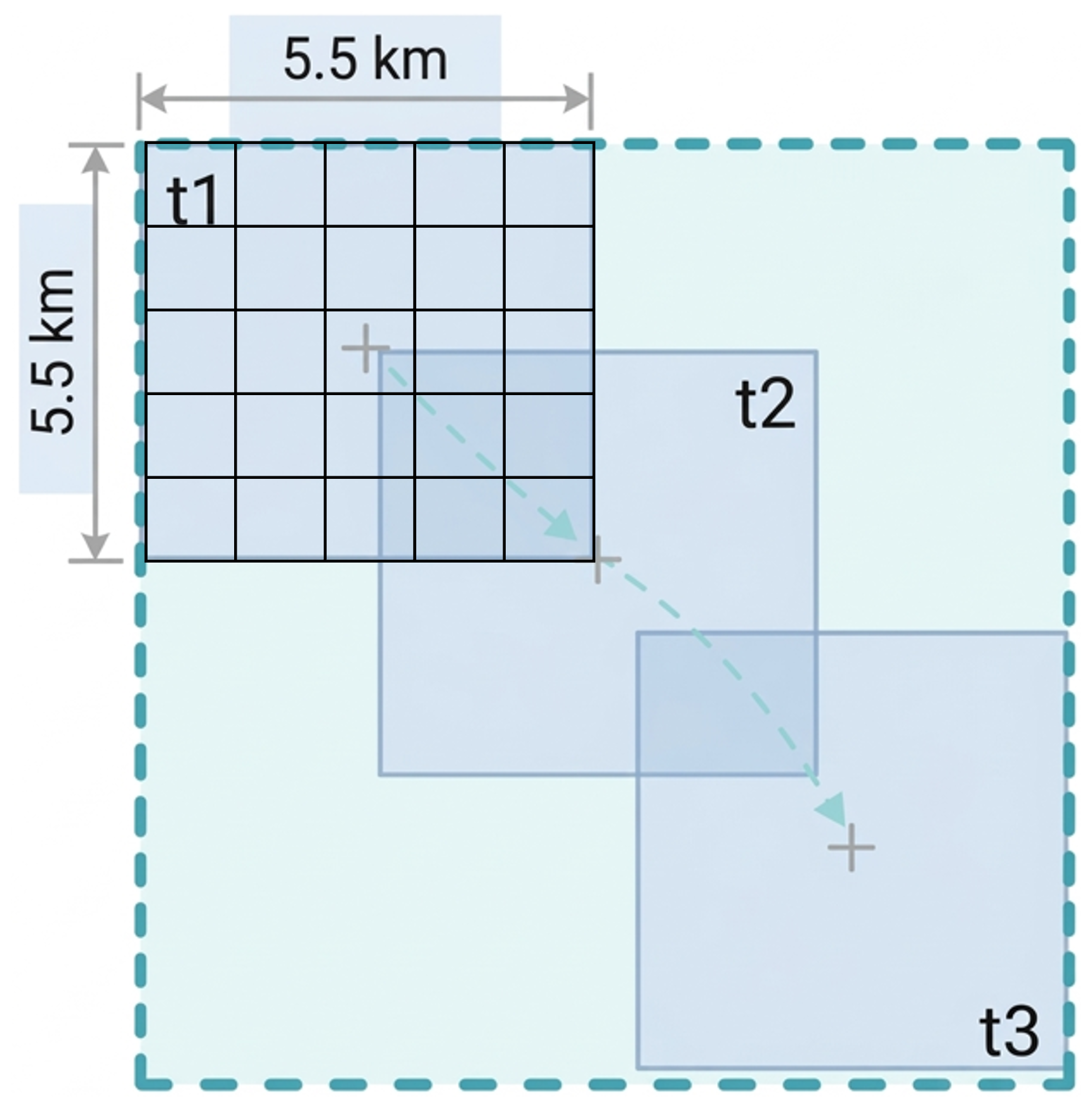
Figure 1 The schematic illustrates the spatiotemporal identification and treatment of a convective target cell during its cumulus stage. The process involves three discrete time intervals (t₁, t₂, t₃) spanning a total of 10 min. For each interval, the maximum updraft is identified (indicated by the “+” markers), and a fixed seeding box of 5.5 km × 5.5 km is centered on this location. For visualization, the t₁ seeding box includes a 5 × 5 grid representing the model's resolution. The final total seeding area (outer dashed perimeter) represents the union of these individual boxes, ensuring the seeding material is consistently injected at the cloud base of the active updraft.

Hailstorms can be relatively small-scale atmospheric features that are often advected with high wind speeds, posing challenges for tracking algorithms. Such rapid movement may result in a lack of spatial overlap between consecutive model output time steps (Brennan et al., 2025). In the tracking algorithm used in this study, hailstorms are identified when specific parameters exceed predefined thresholds. The first is the maximum updraft within a grid column, which helps to distinguish convective clouds from stratiform or stratocumulus clouds (Wood, 2012). The presence of AgI particles, which is the second criterion for tracking, leads us to follow the cells based on the seeding simulations. Accordingly, the CTRL data are masked using the results of the seeding simulations. These thresholds play a significant role in determining which features are tracked and, consequently, influence the results. That is why, in this study, we devote a dedicated section to examining how these thresholds influence the mass of ice, graupel, and hail. In all other sections, the tracking thresholds are fixed at an AgI concentration of 150 L⁻¹ and a maximum updraft velocity in the grid column exceeding 1 m s⁻¹. While literature suggests that updrafts exceeding 10 m s⁻¹ are generally required for sustained hail growth (Knight and Knight, 2001), we employ the tracking threshold of 1 m s⁻¹. This choice is motivated by three factors: first, sensitivity tests show that results on hail size remain consistent regardless of the updraft threshold used (see Fig. S8 in the Supplement). Second, given our 1.1 km horizontal resolution, a threshold of 1 m s⁻¹ is sufficient to identify the core (LeMone and Zipser, 1980); third, a more restrictive threshold would drastically reduce the number of available grid points.

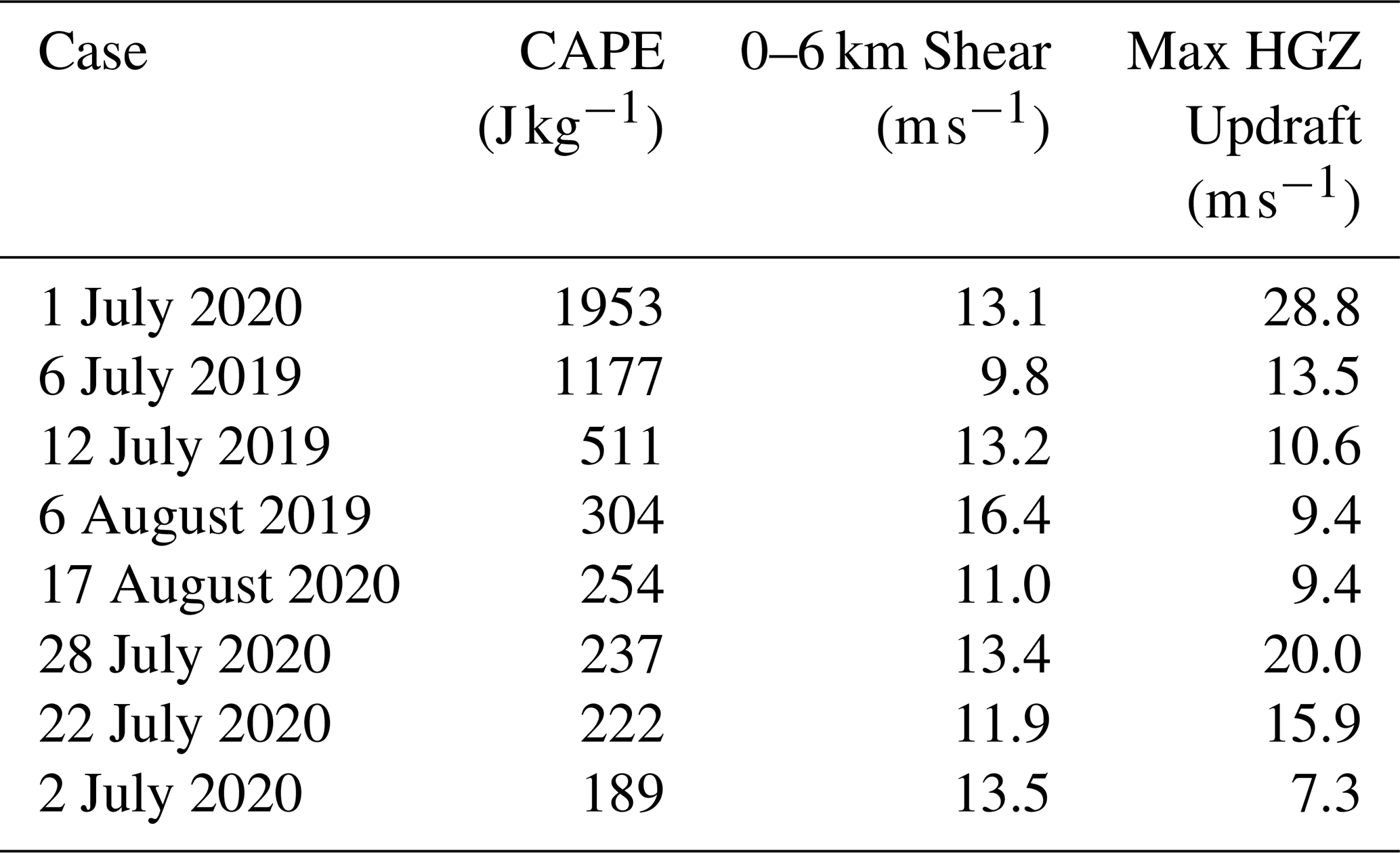
Table 1 Ensemble mean surface-based CAPE (sorted descending), 0–6 km bulk wind shear, and maximum updraft in the hail growth zone (HGZ) for the CTRL hailstorms. Surface-based CAPE and wind shear are computed within a 5.5 km × 5.5 km box centered on the initial tracking point of each hailstorm at the location of maximum CAPE. The maximum updraft is calculated as the peak value reached during the complete evolution of each convective storm.

3 Results

3.1 Case Selection and Overview

To build upon our previous proof-of-concept study (Papaevangelou et al., 2025), we extend the analysis to eight convective storm cases that occurred over Switzerland and southern Germany during the summers of 2019 and 2020. These cases were selected based on the presence of observed hail at the surface. The selected storms span a range of topographic and meteorological environments, characterized by varying CAPE and wind shear values, as well as maximum updrafts in the hail growth zone (HGZ, defined between −10 and −30 °C; Browning and Foote, 1976; Nelson, 1983; Miller et al., 1988) ranging from 7.3 to 28.8 m s⁻¹ (Table 1). These storms occur in settings from moderately complex terrain to high-altitude regions under diverse synoptic conditions (Fig. S1). This variability provides a representative background that allows us to evaluate the robustness of seeding effects across diverse environmental and topographic contexts.

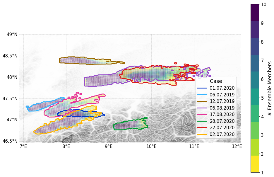
Figure 2 Tracks of the eight studied convective storms. The figure shows the spatial distribution of tracked gridpoints across ensemble members for each case. Tracks are identified using a tracking algorithm that selects grid columns where the maximum updraft exceeds 1 m s⁻¹ and the AgI concentration within the cloud is greater than 150 L⁻¹. Different line colors represent different storm dates, and the color bar indicates the number of ensemble members (1–10) that meet the tracking criteria at each location. The cases in the legend are ordered by CAPE, from highest (top) to lowest (bottom). The grayscale shading represents the terrain.

Specifically, seven cases occurred over moderate topography, while one case (28 July 2020) was located over high-altitude terrain. Across all cases, the ensemble simulations exhibit substantial variability in the spatial distribution of the tracked grid points, as shown in Fig. 2, particularly during the later stages of the convective storms. This variability reflects the sensitivity of convective storm evolution to small perturbations in the initial temperature field, which leads to divergent storm tracks among ensemble members as time progresses. In other words, the locations and extents of the convective cores that meet the tracking criteria differ significantly between members. This is consistent with the findings of Hohenegger and Schär (2007), who showed that errors in convective-scale forecasts grow much faster than those in larger-scale forecasts, due to the high sensitivity of moist convection to small atmospheric changes.

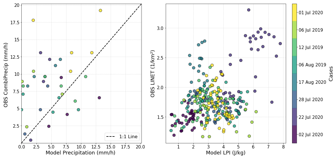
Figure 3 Scatterplots illustrating the comparison of model output with observational data for the studied cases. (Left): Comparison of model precipitation (mm h⁻¹) with the CombiPrecip dataset (mm h⁻¹). (Right): Model-simulated LPI (J kg⁻¹) vs. LINET lightning density (km⁻²). The analysis for each case is performed over a domain centered on the simulated convective storm, extending 1° south/north and 1° west/east from the storm center. Cases are color-coded according to their CAPE values (ranked from highest: yellow to lowest: dark purple).

3.2 Comparison of the Control Simulations with Observations

In this section, we compare the modeled precipitation with the CombiPrecip dataset from MeteoSwiss (2017) and the Lightning Potential Index (LPI) (e.g., Brülisauer et al., 2025) with the low-frequency (VLF/LF) international lightning detection network LINET (e.g., Nag et al., 2015). CombiPrecip provides hourly precipitation fields derived from a geostatistical combination of rain-gauge measurements and radar estimates. The dataset extends 100–150 km beyond the Swiss border, covering neighboring countries, which makes it well-suited for our analysis. Another advantage is its spatial resolution of 1 km, which matches that of our model output. As shown in Fig. 3 (left panel), despite the limited number of data points and considerable spread, it is evident that COSMO tends to underestimate precipitation. This finding is consistent with Shrestha et al. (2022), who used a similar model setup. Furthermore, Fig. 3 (right panel) compares the modeled LPI with the LINET dataset. The LPI evaluates the potential for charge separation by combining updraft speeds with cloud hydrometeor data (graupel, ice crystals, snow, supercooled droplets, and raindrops), whereas LINET monitors lightning activity across most of Europe, including Switzerland and Germany. Notably, the 5 min temporal resolution of the LINET data matches the temporal resolution of our model output. Although the two datasets utilize different units, this comparison demonstrates that the observed lightning activity occurred within the same domain and during the same time periods as the simulated convective storms, albeit with spatial spread. Thus, the simulated storms and their broader environment are broadly comparable to the observed storms, despite the underestimation of precipitation.

3.3 Microphysical and Dynamical Responses to Cloud Seeding

Figure 4 presents the time evolution of the mean vertically integrated cloud ice. In the CTRL simulations, mean vertically integrated ice exhibits substantial variability across cases and ensemble members, as illustrated by the spread. For instance, the 95th percentile reaches 0.2 kg m⁻² after 0.75 h of tracking, while the 5th percentile remains below 0.025 kg m⁻² throughout the entire tracking period. The median across all 80 simulations peaks at the first hour of tracking. Differences between the SEED and CTRL simulations reveal a clear pattern during the initial 1.5 h: the majority of simulations show an increase in cloud ice in the convective clouds following seeding, with a median increase of approximately 0.03 kg m⁻². Beyond 1.5 h, the median difference approaches zero, suggesting that the ice content in the seeded clouds converges with that of the CTRL simulations. After 1.2 h, 2 of the 8 cases, are no longer tracked by the tracking algorithm as they fall below the AgI or updraft threshold. Overall, this consistent increase in vertically integrated ice mass following seeding is in line with earlier findings (e.g., Schaefer, 1946; Vonnegut, 1947).

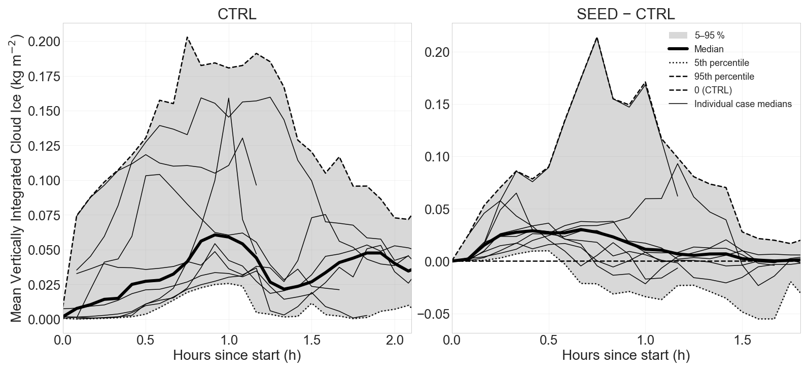
Figure 4 Time evolution of the mean vertically integrated cloud ice values. The left panel shows results from the CTRL simulations, while the right panel presents the difference between SEED and CTRL simulations (SEED–CTRL). The thick black line indicates the median, and the shaded area represents the 5th–95th percentile range across the 80 simulations (8 cases, each consisting of 10 ensemble members) in each category (CTRL or SEED). Thin black lines denote the medians of the individual cases.

Figure 5 presents the vertical profiles of the mean updraft (m s⁻¹) – based on data averaged over the first 1.2 h of the tracking period, during which all cases are tracked (Fig. 4) – and the ice mass fraction in the mixed-phase layer for each of the eight convective cases for the ensemble median. The ice fraction is calculated as:

$$\text{Ice\hspace{0.17em}\hspace{0.17em}Mass\hspace{0.17em}\hspace{0.17em}Fraction}={\displaystyle \frac{M_{\text{ice}}}{M_{\text{water}}+M_{\text{ice}}}}$$

where M_ice is the total ice mass (sum of all frozen hydrometeors except snow, which was excluded due to its negligible contribution relative to the other hydrometeors) and M_water is the total liquid-water mass (cloud water and rain).

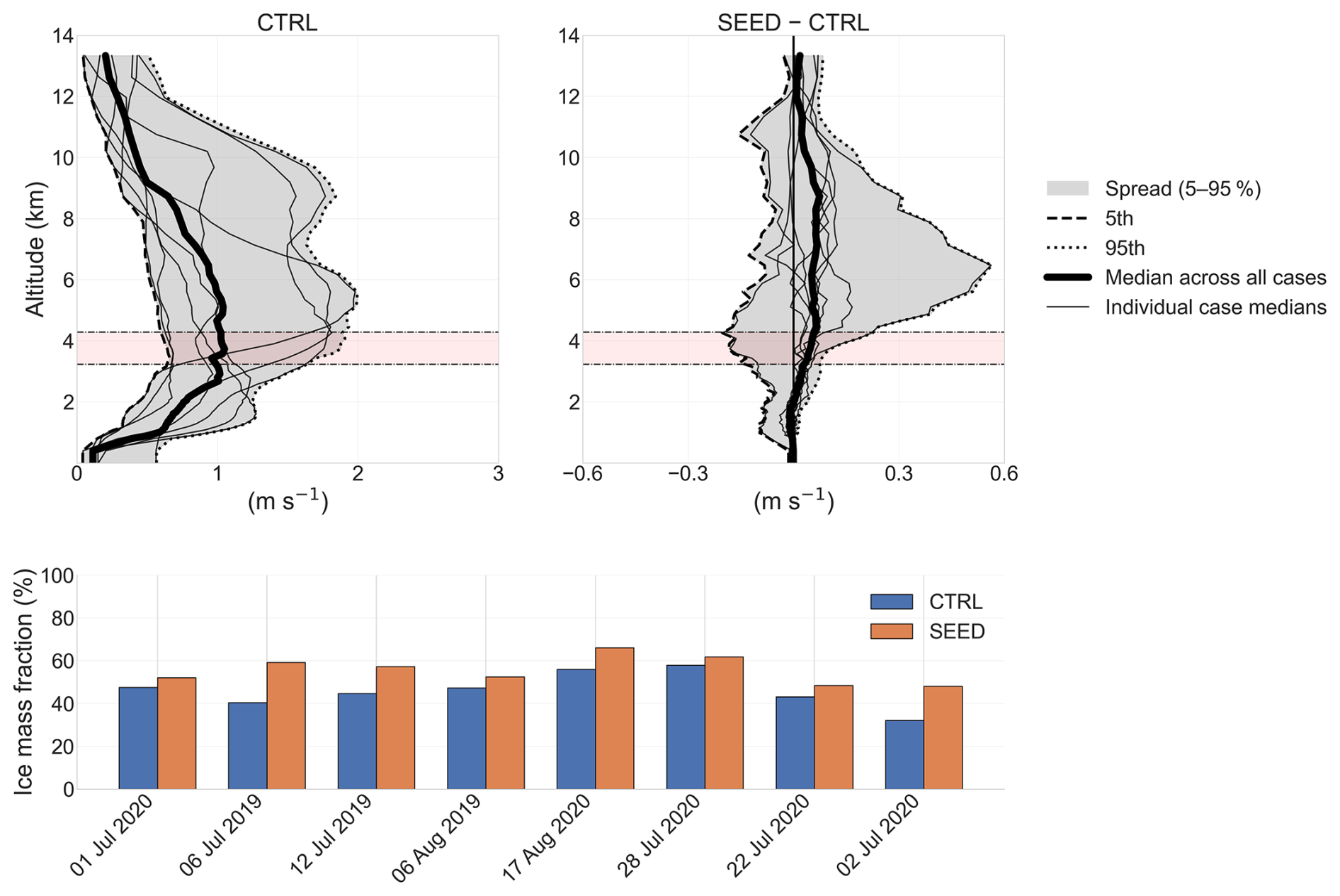
Figure 5 Top: vertical profiles of the mean updraft. The figure shows the spatial mean over the first 1.2 h of tracking for the studied convective storms. Only data from this initial 1.2 h period are included in the averaging, corresponding to the time window in which all cases are tracked. The dashed line indicates the 5th percentile, the dotted line the 95th percentile, and the thick black line represents the median of the simulations. The thin black lines indicate the median for each individual case. The left panel shows the CTRL simulations, while the right panel shows the difference between SEED and CTRL. The red shading marks the vertical range within which the 0 °C isotherm is located across all 80 simulations. Bottom: ice mass fraction (%) in the mixed-phase layer for each of the eight convective cases, shown for the ensemble medians. Values are computed as the ratio of total ice mass to total condensate mass. Results are presented for both the CTRL and SEED simulations, with cases sorted in descending order of environmental CAPE.

The CTRL vertical profile of the mean updraft (Fig. 5, top) increases from the surface to the mid-troposphere, where it reaches its maximum, and then approaches zero near 13 km at the cloud tops of the studied storms. The spread – reaching about 1.5 m s⁻¹ in the mid-troposphere – indicates substantial variability in updraft strength among the eight cases and the ensemble members.

In the seeded simulations (Fig. 5, bottom), AgI consistently increases the ice fraction within the mixed-phase layer, reflecting a systematic shift of condensate from liquid to ice due to enhanced ice nucleation from AgI particles and riming. This increase ranges from 3.8 % to 18.8 %. Examination of the vertical profiles and the SEED–CTRL differences shows that, in most cases, the increase in ice fraction is accompanied by stronger mean updrafts from the 0 °C level up to approximately 10 km. Consistent with the findings of Varble et al. (2023), our simulations suggest that the latent heat of fusion released during enhanced riming and ice nucleation dominates over any updraft-weakening mechanisms, producing a weak but systematic enhancement of the mean updraft in the majority of the simulations.

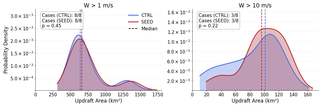
Figure 6 Probability density functions (PDFs) of the updraft areas for the control (CTRL, blue) and seeded (SEED, red) simulations. These distributions aggregate convective cores across 10 ensemble members from up to 8 simulated cases, depending on the threshold. Vertical dashed lines denote the median value of each distribution. The number of cases contributing to each panel is indicated, along with the p value derived from the Mann–Whitney U test.

Figure 6 shows the updraft area distributions for the > 1 and > 10 m s⁻¹ thresholds in the CTRL and SEED simulations. For the > 1 m s⁻¹ threshold, seeding slightly alters the shape of the distribution while maintaining its bimodal structure. The median area is 640 km² for the CTRL and 661 km² for the SEED simulations; however, these changes are not statistically significant according to the Mann–Whitney U test (p=0.45). This non-parametric test was selected because the pooling of the data results in unpaired distributions of unequal sizes, precluding a direct one-to-one comparison. Conversely, for the > 10 m s⁻¹ updraft threshold, seeding modifies the shape of the distribution by slightly increasing the peak and reducing the probability density for updraft areas below 70 km². Although the median area shifts from 101 km² (CTRL) to 96 km² (SEED), these differences are also not statistically significant (p=0.22). Consequently, while we observe updraft invigoration in our simulations, there are no significant changes in the overall updraft area in response to seeding.

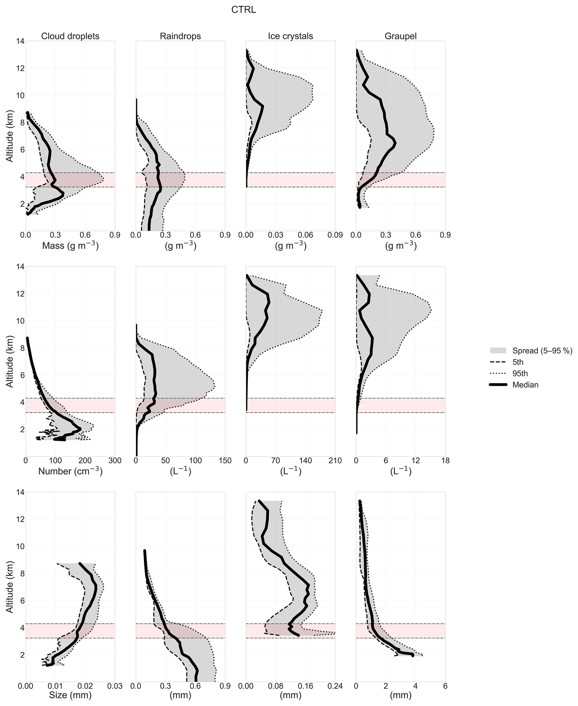
Figure 7 Similar to Fig. 5 (top), but now showing vertical profiles of cloud droplets, raindrops, ice crystals, and graupel. The top row displays mass concentration, the middle row shows number concentration, and the bottom row presents hydrometeor sizes for the CTRL simulations.

Figure 8 Similar to Fig. 7, but now showing the difference due to seeding (SEED-CTRL).

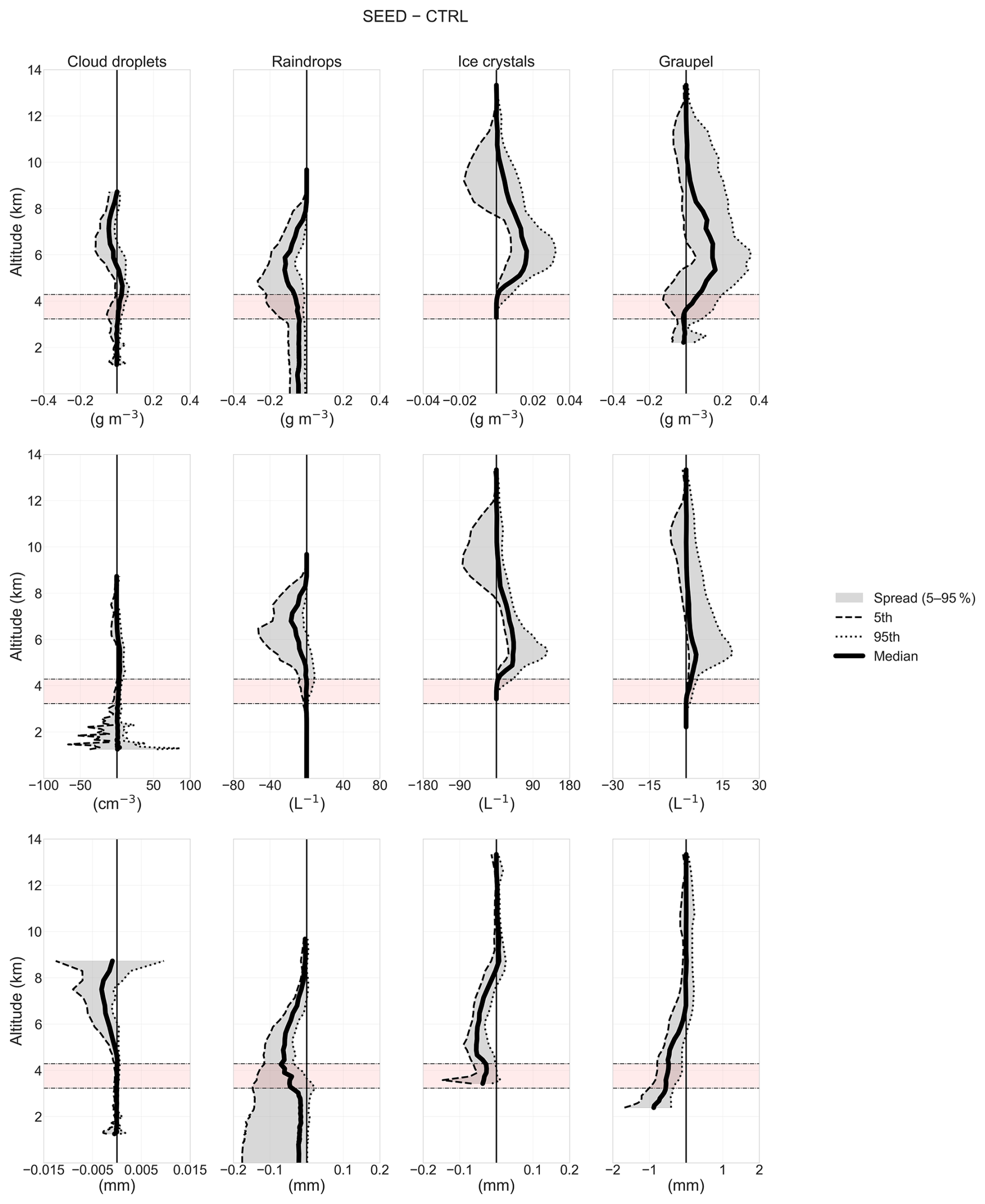
Figures 7 and 8 show vertical profiles of hydrometeor types – cloud droplets, raindrops, ice crystals, and graupel – averaged spatially and temporally (over the first 1.2 h) for both CTRL simulations and the SEED–CTRL differences. The analysis of both figures proceeds sequentially, beginning with cloud droplets, followed by raindrops, ice crystals, and graupel, starting with the CTRL results and then examining the SEED–CTRL difference.

3.3.1 Cloud Droplets

In Fig. 7, cloud droplet mass concentration reaches its maximum just below the 0 °C isotherm. The 0 °C isotherm region exhibits the largest spread in cloud droplet mass concentrations among ensemble members and cases. A similar pattern is evident in the number concentration of cloud droplets, consistent with the mass concentration profile. Median values range between 100 and 200 cm⁻³ below the 0 °C isotherm and decrease steadily toward cloud top. The spread in number concentration is largest below the 0 °C isotherm. The minimum altitude at which cloud droplets appear in most cases is slightly below 2000 m, indicating the mean cloud-base height during the 1.2 h averaging period. In contrast, cloud droplet sizes follow a different vertical profile: mean diameters increase from cloud base to altitudes exceeding 7 km due to growth by condensation and collision–coalescence, then decrease toward cloud top as a result of freezing. Sizes range from 6 to 25 µm, with the upper bound approaching the transition to drizzle-sized drops (Böhm, 1992).

The response of cloud droplets to seeding is weak between approximately 3.8 and 5.5 km, near and just above the 0 °C isotherm (Fig. 8). However, the majority of simulations in this layer shows that cloud droplets gain some mass. This behavior occurs at temperatures just below freezing, where the frozen fraction of AgI remains below 0.1 (Fig. S2). In this layer, seeding produces very few additional ice crystals, so the uptake of water vapor by the ice phase is weak. As a result, most excess vapor condenses onto cloud droplets. This is consistent with the number–concentration profiles, which show that droplet numbers remain essentially unchanged. Above 6 km, AgI particles promote the formation of additional ice crystals, initiating the Wegener–Bergeron–Findeisen process (Wegener, 1911; Bergeron, 1935; Findeisen, 1938). In this regime, cloud droplets lose mass while their number remains nearly constant, as excess vapor deposits onto ice particles, allowing them to grow further. This reduction in droplet mass concentration, together with the nearly unchanged number concentration, results in smaller droplet sizes above 6 km in most simulations. Below 6 km, no systematic seeding signal is evident in the cloud droplet size profiles.

3.3.2 Raindrops

In Fig. 7, raindrop mass concentration ranges between 0.1 and 0.5 g m⁻³. The median values reach their maximum near the 0 °C isotherm, while toward the surface and cloud top, the mass decreases. A similar pattern is evident in the number concentration of raindrops, with the median peaking in the supercooled region where raindrops are smaller in size. In this region, concentrations range from 20 to 130 L⁻¹. Raindrop diameters increase toward the surface as they gain mass through collision–coalescence with cloud droplets and other raindrops. Maximum raindrop sizes in these averaged vertical profiles range between 0.5 and 0.8 mm.

The seeding signal is consistent across mass concentration, number concentration, and size profiles (Fig. 8). In all seeded simulations, raindrops lose mass from the surface up to 8 km. Their number concentration decreases from the 0 °C isotherm to slightly above 8 km, while their sizes are reduced throughout the depth of the convective clouds. This behavior can be explained by riming: numerous newly formed ice particles collide with raindrops, accreting liquid water and transferring mass to the ice phase. As a result, raindrops become fewer and smaller, while ice particles grow through riming. This mechanism also explains our previous findings (Papaevangelou et al., 2025), where AgI seeding delayed the onset of precipitation. In the seeded clouds, smaller and less numerous raindrops take longer to fall against stronger updrafts, thereby delaying rainfall initiation.

3.3.3 Ice Crystals

In Fig. 7, ice crystal mass concentration is about one order of magnitude lower than that of cloud droplets, raindrops, and graupel. However, their number concentration is of the same order of magnitude as raindrops, reaching up to 160 L⁻¹. In the CTRL simulations, both the mass and number concentrations of ice crystals increase significantly above 6 km. Median ice crystal diameters range from 6 to 200 µm.

In the SEED–CTRL differences (Fig. 8), the seeding signal is consistent across all ensemble members and cases. Seeding with AgI increases both mass and number concentrations of ice crystals starting at 5 km – about 1 km lower than in the CTRL simulations – highlighting the ice nucleation ability of AgI at relatively warm temperatures (Fig. S2). This enhancement persists up to 8 km. This reflects additional ice nucleation triggered by AgI particles, producing more numerous ice crystals in the lower and mid-levels of the convective cloud. Seeding also affects ice crystal sizes below 8 km: the larger population of ice particles increases competition for available water vapor, thereby reducing their mean size. Thus, AgI seeding systematically shifts condensate from fewer, larger ice crystals to a more numerous population of smaller ones.

3.3.4 Graupel

In Fig. 7, graupel mass concentration follows a similar vertical pattern to that of ice crystals, but the increase begins near the 0 °C isotherm. The behavior of graupel differs from ice crystals in terms of number concentration: Graupel number concentrations are typically around 10 L⁻¹, whereas ice crystal concentrations are about one order of magnitude higher. Regarding sizes, graupel mean diameters increase toward lower altitudes as particles grow through riming. In the warm layer closer to the surface, graupel eventually melts and transforms into raindrops.

The seeding signal resembles that of ice crystals but appears at slightly lower altitudes within the convective clouds (Fig. 8). Seeding with AgI consistently increases both mass and number concentrations of graupel from the 0 °C level up to 8 km. This enhancement reflects intensified riming, as newly formed ice crystals accrete supercooled liquid water and grow into graupel. The larger graupel population also affects particle sizes below 6 km: increased competition for liquid water limits individual growth, leading to smaller mean sizes. Thus, AgI seeding promotes a systematic shift toward more numerous graupel particles formed by riming, while simultaneously constraining their growth through competition for supercooled liquid water.

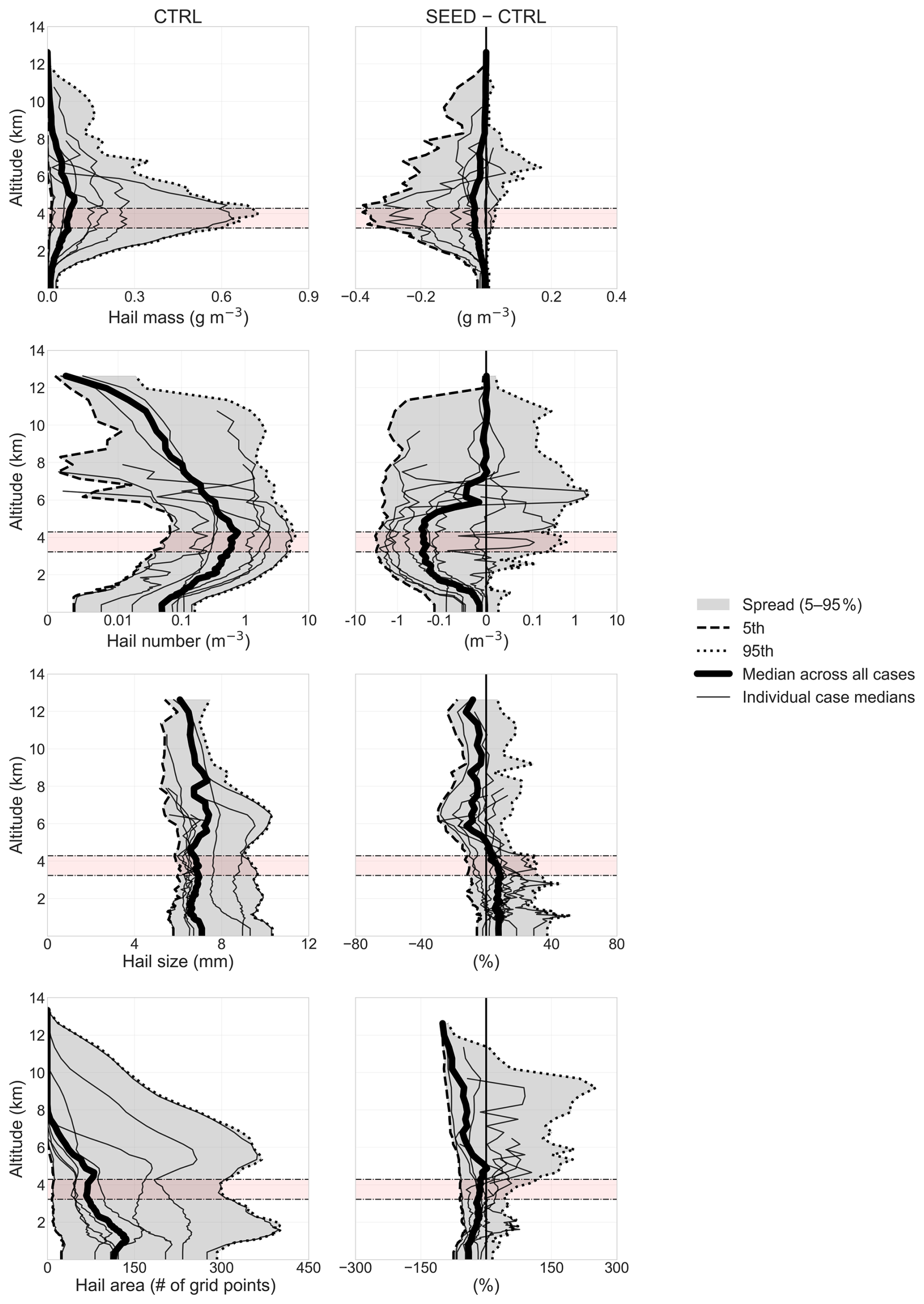
Figure 9 Similar to Figs. 7 and 8, but for hail. First row: hail mass concentration (g m⁻³), second row: hail number concentration (m⁻³), third row: mean hail diameter (the SEED–CTRL panel shows the relative difference, %), fourth row: number of grid points containing hail (the SEED–CTRL panel shows the relative difference (%); for the percentage calculation, at least 10 grid points with hail are required in the CTRL simulations). The left column corresponds to the CTRL simulations, while the right column shows the SEED–CTRL differences. Per-case medians are also included. The x axis for the hail number concentration is shown on a symmetrical logarithmic scale.

3.3.5 Hail

Figure 9 presents the vertical profiles of hail mass concentration, hail number concentration, mean hail diameter, and the number of grid points containing hail, the latter serving as a proxy for the horizontal area affected by hail.

Hail mass concentration in the CTRL simulations shows substantial variability among the eight cases, with the largest spread occurring near the 0 °C isotherm, where values range from nearly zero to about 0.6 g m⁻³. In the SEED–CTRL differences, hail mass in most simulations is equal to or lower than in CTRL simulations from the surface up to roughly 4 km, and the median difference remains slightly negative up to 6 km. This pattern suggests that the enhanced production of ice crystals and graupel following AgI seeding limits the availability of supercooled liquid water for hail growth. However, the seeding signal on hail mass is considerably weaker than the more coherent responses observed for ice crystals and graupel.

Hail number concentration in the CTRL simulations also exhibits large case-to-case variability, with maxima near the melting layer reaching roughly 6 m⁻³. In the SEED–CTRL differences, the median number concentrations decrease from the surface up to 6 km in most simulations. This reduction reflects increased competition for supercooled liquid water caused by the more numerous ice crystals and graupel particles formed during seeding. The sign – though not the magnitude – of this response is consistent with Dessens (1998), who found that heavier seeding reduced hailstone numbers by up to 42 % in physical evaluations in southwestern France. However, the progressively weaker response from ice to graupel to hail in our simulations highlights the increasing microphysical complexity associated with hail formation.

Mean hail diameters in the CTRL simulations range from roughly 5 to 10 mm, representing averages over both the storm's horizontal extent and the 1.2 h tracking period, which naturally smooths localized maxima. In the SEED–CTRL differences, hail size exhibits a mixed response. Above about 5.5 km, the median difference is slightly negative – consistent with the beneficial-competition hypothesis – whereas below this level the signal becomes slightly positive in most simulations, indicating marginally larger hailstones in the lower troposphere. This transition occurs within the supercooled layer, where seeding produces slightly fewer hail particles (Fig. 9). With fewer hailstones competing for cloud-droplet mass – enhanced by invigorated updrafts at this level – and raindrop mass (Fig. 8), riming becomes more efficient for the remaining hailstones, allowing them to grow slightly larger as they descend. However, the substantial spread – containing both positive and negative values throughout the convective cloud – indicates that the seeding effect on hail size is far less systematic than the clearer and more consistent responses seen in the smaller hydrometeors.

We next examine the hail size at the surface. In the CTRL simulations, the median hail diameter is 7.1 mm, with a 5th–95th percentile range of 5.8–10.3 mm. In the SEED simulations, the median increases to 7.6 mm, and the corresponding 5th–95th percentile range broadens significantly to 5.5–14.2 mm. This corresponds to a median SEED–CTRL difference of 7.6 %, with the 5th–95th percentile ranging from about −5.6 % to +37.4 %. Using the terminal fall-speed relation for hail from Mitchell (1996), U_T=11.45(0.1D)^0.5, where D is the equivalent diameter in mm, the kinetic energy scales approximately with the fourth power of the diameter. Accordingly, a 7.6 % increase in diameter yields an increase of 31.3 % in kinetic energy. The associated 5th–95th percentile range implies kinetic energy changes from about −19.1 % below CTRL to more than 261 % above CTRL, indicating substantial case-to-case variability. Despite this spread, 80 % of the simulations show a positive SEED–CTRL signal at the surface, implying that hail kinetic energy increases in the majority of cases. This behavior aligns with the re-analysis of the Swiss Grossversuch IV experiment, which found that seeding can increase hail kinetic energies in some cases (Auf der Maur and Germann, 2021), contrary to the reduction expected from the beneficial-competition hypothesis.

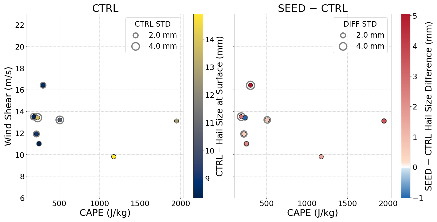
Figure 10 Scatter plots illustrating the impact of AgI cloud seeding on hail sizes for cases categorized by CAPE (J kg⁻¹) and wind shear (m s⁻¹). Left panel (CTRL): surface hail size. To focus on the mature, heavily precipitating stage, we use the 99th percentile over time of the spatial mean. This spatial average is calculated over the tracked convective storms. Plotted values are ensemble means. Right panel (SEED–CTRL): change in hail size between seeded and control simulations. Marker sizes in both panels correspond to the standard deviation across the ensemble members.

Finally, the hail area also exhibits a measurable response to seeding (Fig. 9). In the CTRL simulations, the number of grid points containing hail varies substantially among cases, reaching up to about 400. In the SEED–CTRL differences, the supercooled region shows considerable variability, with AgI either increasing or decreasing the hail-covered area depending on the case, although the median generally remains negative. At the surface, the CTRL simulations show a median of 114 grid points containing hail (5th–95th percentile range: 24–292). In the SEED simulations, the median decreases to 69 grid points, with a 5th–95th percentile range of 6–334. The corresponding SEED–CTRL differences indicate a median reduction of 39.8 %, with a wide 5th–95th percentile range spanning from about −74.9 % to +14.3 %. Moreover, 92.4 % of all simulations show that seeding reduces the hail-covered area at the surface. Thus, although most simulations exhibit a decrease in hail-covered area, the magnitude of the response varies substantially among cases. This behavior is qualitatively consistent with the Alberta hail operational program, where a ten-year radar evaluation found that seeded hailstorms generally produced smaller hail areas than unseeded storms in most cases (Pirani et al., 2023).

3.4 Sensitivity of AgI Cloud Seeding on Hail as a Function of CAPE and Wind Shear

Figure 10 presents scatter plots of the spatial and temporal mean of hail sizes at the surface for each case, classified according to CAPE and 0–6 km wind shear. In the CTRL panel, hail sizes span a wide range, from 8.3 to 14.9 mm. Notably, there is no clear relation between higher CAPE values and larger hail sizes. This suggests that CAPE alone is not a sufficient predictor of severe hailstorms (Lin and Kumjian, 2022). Relatively large hail sizes are observed even in cases with CAPE below 1000 J kg⁻¹, which typically corresponds to weak instability during summer months (NOAA, 2025). Similarly, no consistent pattern is evident with respect to 0–6 km wind shear. The largest mean hail sizes are associated with wind shear values between ∼ 10 and 13.5 m s⁻¹, which, according to Markowski and Richardson (2010), falls within the multicell storm category. Additionally, most cases exhibit substantial variability among ensemble members, as indicated by the marker sizes. In the SEED–CTRL panel, the response of hail to AgI cloud seeding is consistent with what we observed in Fig. 9. Seeding reduces the mean hail size only in one case, with CAPE of 237 J kg⁻¹ and wind shear of 13.4 m s⁻¹, where a decrease of about 1 mm is found. Conversely, in all other cases, seeding increases the mean hail size by up to 5.1 mm, and no clear pattern emerges that links the seeding impact to either CAPE or wind shear. Overall, this figure reinforces our findings in the previous section, where seeding – in the majority of cases and simulations – increases hail sizes and, consequently, hail kinetic energies.

Figure 11 Same as Fig. 10, but showing the number of grid points with hail at the surface.

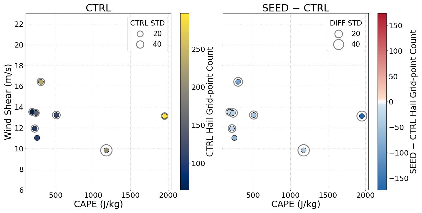
Figure 11 displays scatter plots of the number of grid points with hail at the surface and, similarly to Fig. 10, classifies the cases according to CAPE and wind shear. In the CTRL panel, the highest number of hail-producing grid points is found in the case with the largest CAPE value (296 grid points). However, as in Fig. 10, no consistent pattern emerges indicating that higher CAPE results in a larger spatial extent of hail. The same applies to wind shear: the cases with the most extensive hail coverage correspond to wind shear values of approximately 10 and 16.4 m s⁻¹. In the SEED–CTRL panel, the effect of AgI cloud seeding is consistent across all cases: every case shows a decrease in the number of hail-producing grid points. The largest reduction occurs in the case with the highest CAPE, but there is no evidence that the magnitude of the reduction is systematically related to either CAPE or wind shear. Overall, these results are consistent with our earlier findings: seeding increases the mean hail size in most cases while simultaneously decreasing the spatial extent of hail.

3.5 Impact of Tracking Thresholds on Vertically Integrated Masses of Ice, Graupel, and Hail

In this chapter, we analyze the impact of the AgI and updraft thresholds applied in our tracking algorithm on the vertically integrated masses of ice, graupel, and hail. Figure S3 shows that in the CTRL panel, an increase in the threshold updraft within the grid column specified for tracking leads to an increase in the vertically integrated cloud ice mass. This relationship can be explained by two key processes. First, stronger updrafts activate more CCN, as described by the Segal and Khain (2006) parameterization. These activated droplets are then advected into the mixed-phase region of the cloud, where they freeze and contribute to the cloud ice mass. Second, stronger updrafts loft larger droplets and keep them suspended for longer periods, allowing them to grow through condensation and collision–coalescence before freezing. Once frozen, these supercooled droplets significantly enhance the total ice content in the cloud. In the CTRL simulations, where no seeding is applied, the AgI threshold affects only the number of grid points included in the analysis and the spatial domain, which is defined based on the SEED simulations. Since AgI particles are absent in the CTRL simulations, varying the AgI threshold does not influence the vertically integrated cloud ice mass in a consistent way. Additionally, the highest values of vertically integrated cloud ice mass are found in the case with the second-lowest CAPE, indicating that there is no direct correlation between the ice content of a convective cloud and CAPE.

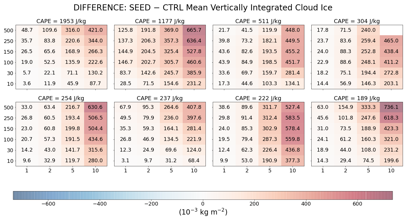
Figure 12 Vertically integrated cloud ice values averaged over time, and the tracked cells for all cases, sorted by CAPE (indicated above each heatmap). The panels show the difference between SEED and CTRL simulations of mean vertically integrated ice values (10⁻³ kg m⁻²) for the ensemble means of the eight cases studied. The x axis represents the updraft threshold (m s⁻¹), and the y axis represents the AgI threshold (L⁻¹). Numerical values within the heatmaps correspond to the colorbar values and are included for improved clarity. White cells denote missing data (NaN).

In the SEED–CTRL panel (Fig. 12), the pattern is clear: seeding increases the vertically integrated cloud ice mass irrespectively of the chosen thresholds. The applied thresholds influence the magnitude of this change, without altering its overall direction. As for the CTRL simulations, the difference in cloud ice mass increases more when only considering grid points with higher updraft thresholds. The maximum differences are observed for the highest updraft and highest AgI concentration thresholds. This robust outcome reinforces the conclusion drawn from Fig. 8, where we showed that AgI particles effectively act as ice-nucleating particles. Through immersion freezing, they enhance ice production in seeded clouds regardless of the selected tracking thresholds.

Figure 13 Same as Fig. 12, but showing vertically integrated graupel mass.

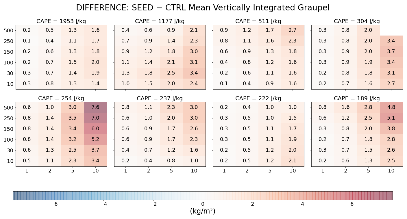
Similarly to Fig. S3, the vertically integrated graupel mass increases when limited to grid cells with higher updraft thresholds (Fig. S4). This is because graupel grows by riming – supercooled liquid droplets accreting onto ice embryos – and stronger updrafts lead to enhanced CCN activation and droplet formation, thereby increasing the amount of supercooled liquid water available for riming, while also prolonging particle residence time in the mixed-phase region (Pruppacher and Klett, 2010; Khain et al., 2005). In COSMO's two-moment microphysics scheme (Seifert and Beheng, 2006), an instantaneous saturation adjustment prevents explicit supersaturation peaks, but droplet number concentrations are nonetheless diagnosed from updraft-dependent aerosol-activation lookup tables (Segal and Khain, 2006), so stronger updrafts still produce more cloud droplets. Thus, even with saturation adjustment, stronger updrafts yield more droplets and thereby enhance graupel production through riming. Interestingly, graupel mass in our simulations does not correlate with CAPE. For example, the maximum simulated graupel mass is 10.1 g m⁻², occurring at a relatively low CAPE value of 237 J kg⁻¹. In the SEED-CTRL plot (Fig. 13), a similar pattern to Fig. 12 is evident. Cloud seeding consistently increases graupel mass across all scenarios. While the magnitude of this increase varies depending on the tracking threshold, the direction of change remains positive. This indicates that the effect of seeding on graupel mass is robust, as also demonstrated in Fig. 8.

A similar pattern is observed for hail such that stronger updrafts yield higher values of total hail mass, reaching up to 2.4 kg m⁻² in the case with 511 J kg⁻¹ CAPE (12 July 2019) (Fig. S5). This increase can be attributed to the same mechanisms discussed in the previous paragraph for graupel – namely, enhanced supercooled liquid water content and prolonged particle residence time in the mixed-phase region. As with graupel, there is no apparent correlation between the vertically integrated hail mass and CAPE, indicating that hail mass is independent of bulk instability.

Figure 14 Same as Fig. 12, but showing vertically integrated hail mass.

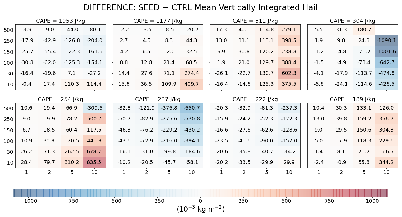
However, the SEED–CTRL panel reveals a more complex pattern (Fig. 14). The impact of AgI seeding on hail mass is strongly case-dependent and varies with the chosen tracking thresholds. Only one case – 28 July 2020, with CAPE of 237 J kg⁻¹ – shows a consistent reduction in hail mass across all tracking thresholds. In all other cases, both the sign and magnitude of the seeding response depend on the specific tracking thresholds applied. This behaviour is consistent with the conclusions drawn before: while the increase in ice and graupel mass following seeding is robust across all cases and all thresholds, the response of hail mass is considerably weaker and far less systematic. This weakening reflects the increasing microphysical complexity associated with hail formation, including variability in residence time, riming efficiency, and competition for available liquid water.

4 Conclusions

This study builds upon our previous case analysis by exploring the complexities of selective cloud seeding, with a particular focus on early updraft seeding in simulated convective storms. This strategy specifically targets convective clouds in their non-precipitating cumulus stage, aiming to influence their microphysical and dynamical evolution. Our investigation centers on six key aspects: cloud droplets, raindrops, ice, graupel, hail and updrafts. We neglect snow because of its minor importance in convective clouds. We also examine whether there is a connection between the seeding impact and two critical meteorological parameters – CAPE and 0–6 km wind shear. In addition, we assess how tracking thresholds affect our conclusions. While acknowledging limitations identified in our previous study – such as the saturation adjustment technique, which may overestimate updraft invigoration following seeding (Grabowski and Morrison, 2021) – our results demonstrate that seeding influences both the hydrometeor fields and the dynamics of the convective clouds. Our key findings can be summarized as follows:

• After seeding with AgI, hail size shows a mixed response at different altitudes. Above about 5.5 km, the median SEED–CTRL difference is slightly negative, consistent with the beneficial-competition hypothesis, meaning that hail size decreases. Below this level, however, the signal becomes slightly positive in most simulations, indicating an increase in hail size. This transition occurs within the supercooled layer above the melting level, where seeding produces slightly fewer hail particles. With fewer hailstones colliding with cloud droplets – which have more mass at these levels due to invigorated updrafts – as well as with raindrops, riming becomes more efficient, allowing the remaining hailstones to grow larger as they descend. At the surface, the median hail size increases by 7.6 %, with a wide 5th–95th percentile range from −5.6 % to +37.4 %. This corresponds to a 31.3 % increase in median hail kinetic energy, with the 5th–95th percentile spanning from −19.1 % to +261 %. Nevertheless, approximately 80 % of the simulations show an increase, indicating that hail size increases at the surface in the majority of the seeded cases.

• The hail-covered area also responds to seeding. The SEED–CTRL differences show a median reduction of 39.8 %, with a wide 5th–95th percentile range from about −74.9 % to +14.3 %. Moreover, 92.4 % of all simulations indicate a decrease in hail area at the surface. Thus, although most simulations consistently show a reduction in hail extent, the magnitude of this response varies substantially among cases.

• In contrast to ice and graupel vertically integrated mass, whose increases after seeding are robust across all tracking thresholds, the vertically integrated hail mass response is substantially weaker and even changes sign depending on the threshold applied. This reflects the greater microphysical complexity of hail formation, including variations in residence time, riming efficiency, and competition for liquid water. Furthermore, no consistent relationship is found between the seeding effect on hail size and hail area and the environmental conditions (CAPE and wind shear), indicating that hail responds to seeding in a strongly case-dependent manner.

In summary, this study provides a model-based assessment of AgI cloud seeding applied to hail-producing convective storms in Switzerland and southern Germany. The results reveal a two-sided response: seeding increases hail kinetic energy in the majority of cases, consistent with findings from the Swiss Grossversuch IV and its subsequent re-analysis (Auf der Maur and Germann, 2021), while it consistently reduces the hail-covered area at the surface across all examined cases and in most simulations, in agreement with the long-term evaluation of the Alberta hail suppression program (Pirani et al., 2023). Although these conclusions are subject to uncertainties inherent to high-resolution simulations – particularly those related to microphysical parameterizations and prescribed INP and CCN conditions – they offer a physically grounded framework for interpreting seeding effects in complex topographic environments such as Switzerland and southern Germany. Looking ahead, meaningful progress will require higher-resolution model simulations, more sophisticated treatments of hail growth and sedimentation, explicit representations of aerosol–cloud interactions, and comprehensive observational datasets to constrain and evaluate model behavior. Such advances will be essential for moving beyond the conceptual framework explored here and for achieving a more complete understanding of how cloud seeding influences hailstorm evolution.