Profiling pollen and biomass burning particles over Payerne, Switzerland using laser-induced fluorescence lidar and in situ techniques during the 2023 PERICLES campaign

Vertical profiles of pollen and biomass burning particles were obtained at the MeteoSwiss station of Payerne (Switzerland) using a novel multi-channel elastic-fluorescence lidar combined with in situ measurements during the spring 2023 wildfires and pollination season during the PERICLES (PayernE lidaR and Insitu detection of fluorescent bioaerosol and dust partiCLES and their cloud impacts) campaign. This original approach provided, for the first time in this region, reliable information on pollen speciation aloft, bridging the gap between ground-based sampling and remote sensing observations. Pollen particles were detected near ground (up to 2 km height), showing strong fluorescence backscatter coefficients (b_F) (up to $\mathrm{8}\times {\mathrm{10}}^{-\mathrm{4}}$ Mm⁻¹ sr⁻¹). Smoke plumes from Canada and Germany were detected at higher altitudes (3–5 km) with lower b_F values compared to those from pollen particles near ground. In situ measurements and in vivo fluorescence spectra were used to classify pollen particles near ground. Ice nucleating particle (INP) concentrations relevant for mixed-phase clouds were enhanced at warm temperatures, characteristic of the contribution of biological particles to the INP population. This was further supported by the correlation between INPs at −14 °C and fluorescent bioaerosol particles detected by the Wideband Integrated Bioaerosol Sensor, while INPs at −20 °C were more strongly linked to coarse-mode dust. Comparison of b_F values from two European Laser Induced Fluorescence lidar stations revealed that aged air masses containing smoke particles exhibited ∼ 50 % lower fluorescence during long-range transport in the free troposphere, possibly due to photochemical aging, mixing with non-fluorescent particles and dispersion.

1 Introduction

Aerosol particles are key components of the atmosphere as they play a crucial role in the Earth radiation budget and climate through scattering and absorbing incoming solar radiation, modulating cloud formation and development, precipitation and the hydrological cycle (Bellouin et al., 2020; Dubovik et al., 2006; IPCC, 2023; Lohmann, 2017; Nenes and Seinfeld, 2003; Stevens and Feingold, 2009). However, large uncertainties remain on the role of aerosols on Earth's climate and radiation forcing (Bjordal et al., 2020; Chen et al., 2022; IPCC, 2023; Lohmann and Lesins, 2002; Seinfeld et al., 2016; Watson-Parris and Smith, 2022). Biological aerosols (or “bioaerosols”) comprise an important and largely understudied type of atmospheric aerosol and include pollen grains, fungal spores, viruses, bacteria, algae, and cell fragments. It is now established that bioaerosols impact ecosystems, cloud formation and possibly climate (Fröhlich-Nowoisky et al., 2016; IPCC, 2023; Violaki et al., 2021, 2025; Wilson et al., 2015); however, there is still a large gap in the scientific understanding of the interaction and co-evolution of life and climate in the Earth system (Fröhlich-Nowoisky et al., 2016). Bioaerosols can act as cloud condensation nuclei (CCN) (Mikhailov et al., 2021; Petters et al., 2009) and ice nucleating particles (INPs) in mixed-phase clouds (Gao et al., 2024, 2025). The latter can occur at relatively warm sub-zero temperatures (∼ −2 to −10 °C), and thus bioaerosols can initiate ice multiplication that leads to rapid glaciation, storm intensification and extreme precipitation (Gao et al., 2025; Lohmann et al., 2016; O'Sullivan et al., 2015).

Pollen grains are ubiquitous in the atmosphere during the pollination period of different flowering plants like trees, grasses and other herbaceous plants. Climate induced-warming over the last decades during winter and spring lead to an earlier onset and increased intensity with a resulting extension in the pollen season (Beggs, 2016; Glick et al., 2021; Lake et al., 2017; Ziska et al., 2019) and exposure of humans to pollen allergens (Albertine et al., 2014; Martikainen et al., 2023; Zemmer et al., 2024).

This prolonged exposure has been linked to a rise in allergic respiratory diseases such as allergic rhinitis and asthma, affecting millions of people worldwide and imposing a growing public health burden, especially in urban environments where interactions with air pollutants can further intensify symptoms (Buters et al., 2018; D'Amato et al., 2020). Understanding the dynamics of pollen emission, transport, and transformation in the atmosphere is thus crucial for improving allergy forecasts and assessing health risks under changing climatic conditions.

Pollen fluorescence spectra analysis is increasingly used to monitor these changes and provide valuable information on biogenic aerosol classifications (pollen, bacteria, fungi) and other aerosol types containing fluorescent materials, such as biomass burning (BB) and dust aerosols, using different light-induced fluorescence techniques based on UV-light sources (LEDs, flash lamps, lasers) (Huffman et al., 2020; Sauvageat et al., 2020; Tummon et al., 2024) and aloft (Reichardt et al., 2025; Richardson et al., 2019; Veselovskii et al., 2023, 2024).

Vertical profiles of fluorescent agents in the lower stratosphere were first detected by Immler et al. (2005) using laser remote sensing (lidar). Later, Sugimoto et al. (2012) detected the presence of fluorescent dust particles with a multi-channel lidar spectrometer (420–510 nm) using laser radiation at 355 nm as an excitation source. Few years later, Saito et al. (2018, 2022) detected pure pollen particles very close to the source, based on the analysis of lidar Laser Induced Fluorescence (LIF) signals and reference pollen fluorescence in vitro spectra obtained with a 355 nm excitation. Richardson et al. (2019) were the first to classify different types of mixed bioaerosols (pollen, fungi, bacteria) in the lower troposphere by spectrally decomposing lidar LIF bioaerosol fluorescence spectra using a 32-channel fluorescence spectrometer (based on in vitro reference fluorescence spectra for specific pollen, fungi, and bacteria) excited at 266 and 355 nm. Veselovskii et al. (2020) combined Mie-Raman and fluorescence (444–487 nm) lidar techniques to detect the presence of fluorescent smoke and dust particles in the troposphere. Later, they extended this approach to characterized atmospheric layers of smoke, dust, pollen and urban particles through a combination of linear particle depolarization ratio, fluorescence coefficient and capacity vertical profiles using single-channel (detection at 444–470 nm) (Veselovskii et al., 2021, 2022a, b) and 5-channel (438, 472, 513, 560 and 614 nm) fluorescence lidar systems (Veselovskii et al., 2023, 2024, 2025). The present study aims to further extend the LIF lidar technique from near ground to the free troposphere by combining the observation systems of Richardson et al. (2019) and Veselovskii et al. (2021). This approach will enable us to classify pollen types near ground (below 300 m above ground level – a.g.l. by using 30° slant laser emission along a nearby mountain upslope) and to characterize atmospheric layers of pollen and smoke in the free troposphere during the PERICLES (PayernE lidaR and in situ detection of fluorescent BB, bioaerosol and dust partiCLES and their cloud impacts) campaign at the MeteoSwiss station of Payerne (46.822° N, 6.941° E, 491 m above sea level (a.s.l.), Switzerland) from May to December 2023. The main objective of this campaign was to understand the spatio-temporal variability of different types of bioaerosols containing pollen, BB and dust within the Planetary Boundary Layer (PBL) and lower free troposphere aloft (typically up to 2–5 km a.s.l.) and their potential role in cloud formation through a combination of fluorescence LIF lidar, radiosonde profiling, and in situ (ground-level) characterization of bioaerosol, air pollutants, chemical composition and INP measurements. Other objectives of this campaign aimed to map the diversity and sources of bioaerosols in the lower atmosphere to provide insights on the mechanisms controlling their concentration near ground, to validate existing pollen forecast models (ICON model) (Zängl et al., 2015) on a semi-rural site. Although the full PERICLES dataset contains a large amount of aerosol episodes, we focus on two, characteristic of long- and near-range transport of BB and pollen particles (occurred during May and June 2023) using a multi-instrumental approach.

A description of the experimental site and the in situ and remote sensing instrumentation implemented during the PERICLES campaign is given in Sect. 2, while, in Sect. 3 we present the methodology used to calibrate the lidar fluorescence channel for the retrieval of the fluorescence backscatter coefficient, and the fluorescence spectra clustering/analysis for pollen classification near ground. Section 4 presents the pollen climatology of the site, while in Section 5 we present the observational results regarding the vertical profiles of the aerosol elastic backscatter and bioaerosols (smoke and pollen) fluorescence backscatter and capacity, obtained during two case studies. We also discuss our results in conjunction with similar data obtained in France and Germany during the same period. Finally, in Sect. 6 we summarize the key findings of this study.

2 Experimental site and Instrumentation

2.1 Site location

The PERICLES campaign took place at the MeteoSwiss station of Payerne, (46.82° N, 6.94° E, altitude 490 m a.s.l., Switzerland), between 1 May and 20 December 2023. The rural site is located on a hilly terrain on the Swiss Plateau, roughly 1 km south from the city of Payerne. It is surrounded by grassland and several farmlands, and close to a forest ecosystem between the Jura mountains and the Alps (Fig. 1a–c). The position of the in situ instrumentation and the lidar is described in Fig. 1d–e. The station is member of the Aerosol, Clouds, and trace gases research Infrastructure-ACTRIS (https://www.actris.eu, last access: 12 June 2025) and hosts a suite of air quality measuring instrumentation of the National Air Pollution Monitoring Network-NABEL of Switzerland, which in turn is part of the European Monitoring and Evaluation Programme (EMEP), and stores its data at EUROAIRNET, which was established by the European Environment Agency (EEA). It is also a GAW regional station for gaseous species, an AERONET and EARLINET station, an ACTRIS station for aerosol in situ and aerosol cloud remote sensing, as well as, a GRUAN and a Network for the Detection of Atmospheric Composition Change (NDACC) station. Payerne is also a SwissMetNet (SMN) station which covers all relevant in situ meteorological parameters.

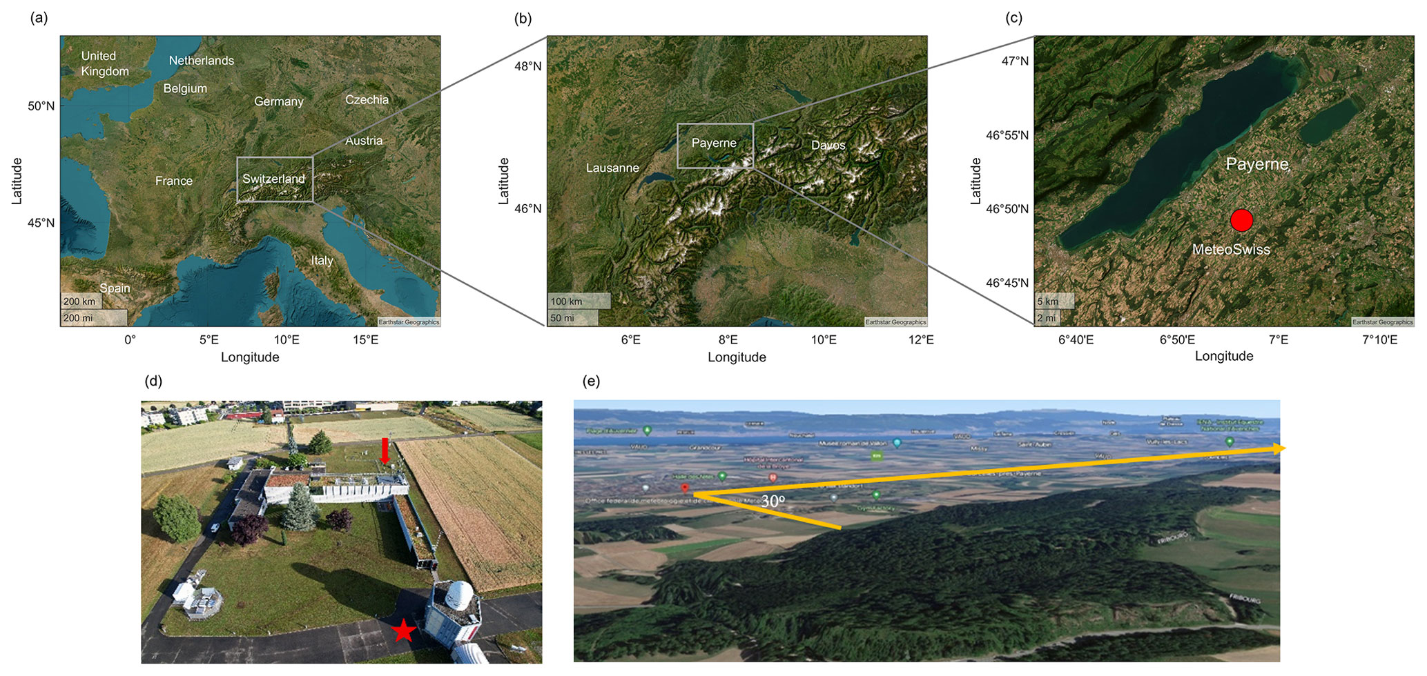
Figure 1 (a) The study area of Switzerland (b) the sub-domain over Payerne (c) the experimental site of MeteoSwiss in Payerne (d) MeteoSwiss in Payerne, the roof of MeteoSwiss is indicated by the vertical arrow and the position of the lidar by an asterisk (e) the emitted laser beam (30° elevation angle to the ground) passing over the nearby hill by 50–200 m (right). © Google Maps 2025.

2.2 Instrumentation

To comprehensively understand the meteorology and general atmospheric dynamical conditions, aerosols, characteristics and potential impact on cloud formation, a large suite of in situ and remote sensing instruments was deployed at the Payerne site (Table S1 in the Supplement). In situ bioaerosol measurements were based on SwisensPoleno (Swisens AG, Lucerne, Switzerland), in parallel with Hirst-type pollen traps that provide a traditional standard for comparison (Crouzy et al., 2016). Furthermore, investigations on the role of bioaerosols as INPs provided important insights on their contribution in cloud formation (Gao et al., 2024, 2025). The remote sensing instrumentation for the detection of non- and fluorescent aerosols was based on a single-wavelength elastic and laser-induced fluorescence lidar system developed by National Technical University of Athens (NTUA), École Polytechnique Fédérale de Lausanne (EPFL) and Foundation for Research and Technology (FORTH), with single or multiple detection channels. All in situ measuring instruments were deployed at the rooftop of the MeteoSwiss building (8 m a.g.l.), except the aethalometer and a Time of-Flight Aerosol Chemical Speciation Monitor (ToF-ACSM), which were located at ground level in the Baseline Surface Radiation Network (BSRN) in a dedicated cabin in the vicinity (∼ 30 m) of the main building, while the remote sensing instruments were located ∼ 70 m away and with an unobstructed view of the in situ measuring devices. Meteorological data (wind speed and direction, relative humidity, temperature) affecting low tropospheric air mass dynamics and mixing were obtained using operational MeteoSwiss SMN station, wind lidar, radar and local radiosoundings.

2.2.1 In situ instrumentation

During the PERICLES campaign, a wide variety of in situ instrumentation were deployed, such as a SwisensPoleno, a Hirst-type volumetric trap, a Wideband Integrated Bioaerosol Sensor (WIBS-5-NEO), an Aethalometer AE-33, ToF-ACSM, a high-flow rate impinger (Coriolis^® micro-μ), as well as an offline droplet freezing assay called DRoplet Ice Nuclei Counter Zurich (DRINCZ). The SwisensPoleno is an all-optical automatic pollen monitoring device using scattered light measurements, digital holography, and light-induced fluorescence to identify and count different pollen types. Firstly, particle size and velocity are determined using scattered light from two trigger lasers. Following this first assessment, two 200 × 200-pixel images are obtained using digital holography at 90° perspectives with a resolution of 0.53 µm. Following the holography module, two light-emitting diode (LED) light sources at 280 and 365 nm, and a laser source at 405 nm excite the sampled particles and produce fluorescence. These spectra are recorded across five different measurement windows (335–380, 415–455, 465–500, 540–580, and 660–690 nm). A blower maintains a sampling airflow rate of 40 L min⁻¹, and a virtual impactor unit that concentrates aerosol particles with diameters larger than 5 µm (Sauvageat et al., 2020). Inference allowing the identification of individual particles is performed in the device itself (embedded computer). A two-step classifier is used: firstly, the size and the overall shape allow to filter out most non-biological coarse aerosol, secondly, convolutional neural networks are used for taxa identification based on holographic images. Note that the first stage of the filter is prone to false-negative when considering fungal spores that show a greater morphological variability than pollen. The classification is evaluated following the procedure of Crouzy et al. (2022). A Hirst-type volumetric trap (Hirst, 1952) was also utilized to identify and count pollen in complement to the automatic monitors at roof level. The Hirst sampler is calibrated at a flow rate of 10 L min⁻¹ and captures pollen grains on a rotating drum covered with Melinex film coated in silicon fluid (Galán et al., 2014; O'Connor et al., 2014; Savage et al., 2017). Each 48 mm on the drum represents 24 h of sampling resulting in a full rotation of the drum in a week. Once the drum is fully rotated the pollen grains are counted, offline, under a light microscope. Daily pollen counts are obtained by running two longitudinal sweeps along the 24 h slide and identifying each pollen type. This manual counting procedure complements the automatic monitors used and serves as a reference measurement, as it allows for the identification of 47 different pollen taxa, albeit at the cost of a reduced temporal resolution and sampling. The Hirst trap has a lower temporal resolution compared to the SwisensPoleno: in the operational longitudinal scanning mode used at MeteoSwiss it shows limitations at the hourly level due to limited sampling efficiency and broad band spreading. However, especially for high pollen concentrations, Hirst samplers can give a hint on the sub daily evolution of the pollen concentration. Hirst performance improves at the daily level but deviations between Hirst traps operating in parallel can still be observed (Adamov et al., 2024). Notably improper calibration of Hirst flow has been documented (Oteros et al., 2017), which may lead to deviations reaching up to 72 %. These factors highlight the limitations in Hirst precision and reliability, especially for fine temporal analyses. Those limitations are currently still balanced by the more precise discrimination capabilities of Hirst measurements compared to the commercially-available automatic instruments.

The WIBS-5–NEO (Droplet Measurement Technologies, LLC., USA), sampling aerosol particles from an omnidirectional total inlet, was employed in parallel with SwisensPoleno and Hirst. The WIBS was used to detect and classify fluorescent biological aerosol particles (FBAPs) by discriminating the fluorescent properties and optical sizes of particles. WIBS first counts and measures particle sizes between 0.5 and 30 µm using a 635 nm laser beam. WIBS triggers the fluorescence emission of particles at 280 and 370 nm wavelengths and then records their fluorescent signals in two wavebands (310–400 and 420–650 nm, respectively). Thus, fluorescent signals at three different channels can be recorded, including FL1 channel detecting the fluorescence emissions in the waveband 310–400 nm of particles excited at 280 nm, FL2 channel and FL3 channel detecting the fluorescence emissions in the waveband 420–650 nm of particles excited at 280 and 370 nm respectively (O'Connor et al., 2014; Savage et al., 2017). The three channels can detect different biologic fluorophores: tryptophan-containing proteins, NAD(P)H co-enzymes and riboflavin (Kaye et al., 2005; Savage et al., 2017), which are ubiquitous in living organisms, including microbes and pollen (Pöhlker et al., 2012). A particle only carrying one type of fluorophores and showing fluorescence in only one of the three channels will be classified to a type of WIBS_A (FL1), WIBS_B (FL2) or WIBS_C (FL3). Similarly, a fluorescent particle detected by two channels will be recorded as an WIBS_AB (FL1 and FL2), WIBS_AC (FL1 and FL3) or WIBS_BC (FL2 and FL3) particle. WIBS_ABC refers to particles having three types of fluorophores and is reported to have the highest probability of being biological origin among all types of particles (Gao et al., 2024, 2025; Hernandez et al., 2016; Savage et al., 2017). Here, we used averaged forced trigger signal plus 9σ to subtract background noise for calculating the fluorescent signal of sampled aerosol particles instead of 3σ used in other studies (Savage et al., 2017), to reduce the influence from interfering particles. In addition, the size distribution of aerosol particles recorded by WIBS was used to calculate the number concentration of total aerosol particles (0.5–30 µm), termed WIBS_total, and coarse mode particles (2.5–30 µm), termed WIBS_coarse.

The mass concentration of equivalent black carbon (eBC), sampled through a PM₁₀ cut-off inlet, was monitored by a dual spot filter-based photometer Aethalometer AE-33 (Magee Scientific, Berkeley, CA, USA), measuring at 7 wavelengths (370, 470 520, 590, 660, 880 and 950 nm) with a time resolution of 1 min (Drinovec et al., 2015; Eleftheriadis et al., 2009; Stathopoulos et al., 2021) and then averaged on an hourly basis. PM₁ organic carbon (OC) and the chemical composition of non-refractory aerosols, including organics, sulphate (SO${}_{\mathrm{4}}^{\mathrm{2}+}$), nitrate (NO³⁻), ammonium (NH${}_{\mathrm{4}}^{+})$ and chloride (Cl⁻), was measured by the ToF-ACSM (Aerodyne Research Inc., USA) with a time resolution of 10 min (Dada et al., 2025; Fröhlich et al., 2015; Zografou et al., 2024). The number concentrations of INPs relevant for mixed-phase clouds for $T>-\mathrm{25}$ °C were measured for 82 samples collected from 8 May to 28 June. The results were linked to the abundance and properties of the observed aerosol particles (e.g., biological particles) to examine the source of INPs and the aerosol-cloud interaction activities of different aerosol sources. Ambient aerosols were sampled for 10 and 60 min using a high-flow rate impinger (Coriolis^® micro-μ, Bertin Instruments, France, 300 L min⁻¹) and collected into 15 mL ultrapure water (W4502-1L, Sigma-Aldrich, US).

The offline droplet freezing assay DRINCZ (David et al., 2019) was used to measure the freezing abilities of sample droplets at different temperatures down to −24 °C. Using the sampled air and liquid volume, as well as dilution rates for preparing DRINCZ droplets, the INP number concentration of a DRINCZ sample was calculated as a function of temperature and the background noise was corrected by analyzing blank samples. Detailed methodology on the INP sampling protocol and DRINCZ data analysis is provided in Gao et al. (2025). The freezing ability of aerosol particles determines their removal process, life time and atmospheric impacts. As such, it is important to evaluate the freezing and cloud interaction abilities of the observed aerosol sources.

2.2.2 Remote sensing instrumentation

Remote sensing instrumentation was used, including a LIF lidar and a multispectral lidar detector, to retrieve vertical profiles of aerosol backscatter (b_aer) coefficients at 355 nm and the corresponding bioaerosol fluorescence backscatter coefficients. The lidar system is based on a pulsed Nd:YAG laser (Lumibird Q-Smart 450) emitting at 355 nm with energy of 130 mJ per pulse at 10 Hz repetition frequency. The UV laser beam is emitted to the atmosphere through a Pelin-Broca prism and a 10 × diameter expander at an elevation angle of 30°, pointing northward and passing at ∼ 50–200 m [relevant (start-end) distance of the laser beam to the surface of the mountain over a nearby hill (cf. Fig. 1, lower right). A 150 mm diameter Cassegrainian telescope (focal length f=1125 mm) was used to collect the backscattered lidar signals and fed them to a filter spectrometer through a SiO₂ optical fiber having a numerical angle NA = 0.2 (cf. Fig. 2). At the entrance of the spectrometer a double achromatic lens (1) collimates the incoming beam, while a dichroic beam splitter (2) reflects the 355 nm lidar signal to a focal lens (7), then to a neutral density filter (6) and to the photomultiplier tube (PMT) eyepiece doublet (5). The elastic lidar signals are filtered by an interference filter (4) centred at 355 nm (FWHM = 0.5 nm), while the LIF lidar signals pass through the dichroic beamsplitter and then through a cut-on long-pass optical filter (3) (FEL0400 Thorlabs GmbH) which transmits all wavelengths greater than 400 nm. An interference filter centred at 470 nm (FF02-470/100-25 Semrock, FWHM = 100 nm) is used to detect the LIF lidar signals between 420–520 nm.

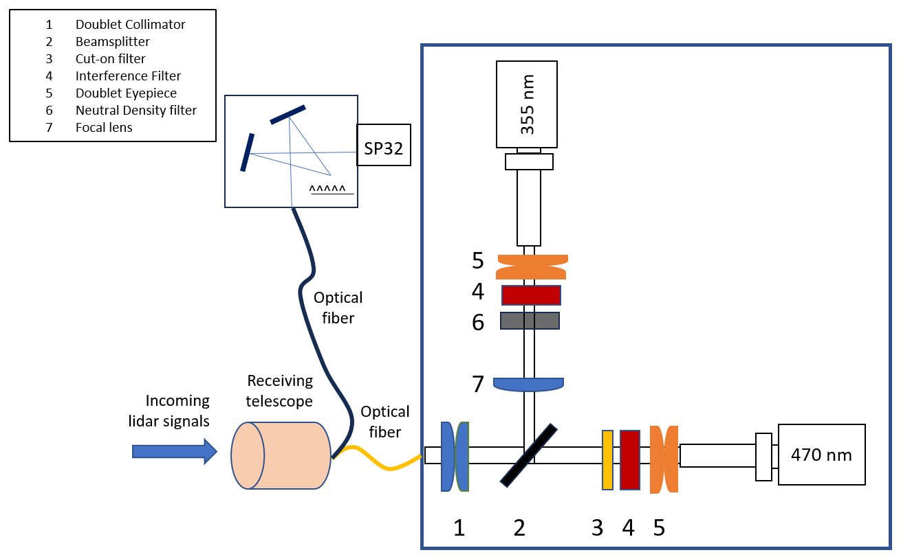
Figure 2 Set up of the elastic-LIF lidar system and the multispectral (SP32) lidar spectrometer: (1) double achromatic lens, (2) dichroic beam splitter, (3) cut-on filter, (4) interference filter, (5) doublet eyepiece, (6) a neutral density filter and (7) focal lens.

An optical fiber placed at the focal length of the receiving telescope is optically coupled to the entrance of a multispectral (32-channel) lidar detector (Licel GmbH) equipped with a holographic grating spectrometer (grating with 1200 grooves mm⁻¹, 400 nm blaze). The LIF lidar signals, after passing through a cut-on long-pass optical filter (FEL0400 Thorlabs GmbH), are detected in the photon counting mode by 32 photocathode elements (PMTs) and spectrally resolved between 420–620 nm with a 6.2 nm spectral resolution (Fig. 2). In all cases, the fluorescence lidar technique is used only during nighttime due to high atmospheric background radiation during daytime.

3 Methodology

3.1 Calibration of the fluorescence channel for the retrieval of the fluorescence backscatter coefficient

To determine the fluorescence backscatter coefficient, we need to consider the lidar signals at two channels: the elastic channel (λ_E=355 nm) and the fluorescence channel (λ_F=470 nm). Since our lidar system is not equipped with a N₂ Raman channel (Veselovskii et al., 2020), we replace the signal of the N₂ Raman channel (P_R) by the signal at the elastic channel (P_E), in order to calculate the fluorescence signal (P_F). Thus, according to Veselovskii et al. (2020) we can write the signals P_F and P_E as following:

$$\begin{array}{}\text{(1)}& {\displaystyle }{P}_{\mathrm{F}}=b_{\mathrm{F}}{T}_{\mathrm{F}}{C}_{\mathrm{F}}\text{(2)}& {\displaystyle }{\mathrm{P}}_{\mathrm{E}}=b_{\mathrm{355}}{T}_{\mathrm{E}}{C}_{\mathrm{E}}\end{array}$$

where, T_F and T_E are the exponential terms of the atmospheric transmissions at the fluorescence and elastic channel, respectively; C_F and C_E correspond to the range-independent lidar calibration constants including the efficiency of the detection channel at wavelengths λ_F and λ_E, respectively (Veselovskii et al., 2020). By dividing Eq. (1) by Eq. (2), the the aerosol fluorescence backscatter coefficient b_F can be obtained:

$$\begin{array}{}\text{(3)}& b_{\mathrm{F}}={\displaystyle \frac{P_{\mathrm{F}}}{P_{\mathrm{E}}}}{\displaystyle \frac{T_{\mathrm{E}}}{T_{\mathrm{F}}}}{\displaystyle \frac{C_{\mathrm{E}}}{C_{\mathrm{F}}}}{b}_{\mathrm{355}}\end{array}$$

To obtain the vertical profile of b₃₅₅ we used the Klett inversion technique (Klett, 1985), using typical lidar ratios at 355 nm of 45 sr for aged BB particles from North American wildfires (Hu et al., 2022; Mylonaki et al., 2021; Ortiz-Amezcua et al., 2017), 50 sr for pollen particles at low altitudes (Veselovskii et al., 2022a) and 60 sr for fresh BB particles from European wildfires and pollen (Burton et al., 2012; Nepomuceno Pereira et al., 2014). The uncertainties of the retrieved b₃₅₅ values, are of the order of 25 %–30 %, based on a sensitivity analysis (for 45 sr < LRs < 60 sr), performed for these three different types of aerosols. The molecular backscatter coefficient at 355 and 470 nm was calculated using a standard atmosphere model by the Global Land Data Assimilation System (GLDAS) (Rodell et al., 2004); thus, the ratio ${\frac{T_{\mathrm{E}}}{T_{\mathrm{F}}}}_{\mathrm{|}\mathrm{mol}}$ for the molecular contribution can be derived. As the particle atmospheric transmission differs little between 355 and 470 nm, we used an appropriate value of the extinction-related Ångström exponent γ equal to 1.16 (Veselovskii et al., 2020), valid for western wildfires measured for the pair 355–532 nm (Janicka et al., 2017) to account for the spectral dependence of the aerosol extinction between wavelengths 355 and 470 nm. As the differential particle transmission for a wavelength separation between 470 and 532 nm is less than 62 nm for low to medium aerosol loads, the induced second order error on ${\frac{T_{\mathrm{E}}}{T_{\mathrm{F}}}}_{\mathrm{|}\mathrm{par}}$ for the particulate contribution remains less than 6 % (Gast et al., 2025).

To calculate $\frac{C_{\mathrm{E}}}{C_{\mathrm{F}}}$ we need to consider the optical transmittances and reflectances of the various optical components (beam splitters, interference and neutral density filters), as well as the detection sensitivities of the PMTs used at the two channels: 355 and 470 nm (Gast et al., 2025). Following Veselovskii et al. (2020), we can write:

$$\begin{array}{}\text{(4)}& {\displaystyle \frac{C_{\mathrm{E}}}{C_{\mathrm{F}}}}={\displaystyle \frac{R{T}_{\mathrm{ransE}}}{F{T}_{\mathrm{ransF}}}}{\left[{\displaystyle \frac{P_{\mathrm{E}}}{P_{\mathrm{F}}}}\right]}_{\mathrm{an},\mathrm{cal}}\end{array}$$

where R is the reflectance of the dichroic beamsplitter (Fig. 2), while T_ransE and T_ransF are the transmittances of the optical elements of the LIF spectrometer at 355 and 470 nm, respectively (cf. Table 1). Using the values of the transmittance at channels 355 and 470 nm we have: $T_{\mathrm{ransE}}=T_{\mathrm{1}}{T}_{\mathrm{3}}=\mathrm{0.445}$ and $T_{\mathrm{ransF}}=T_{\mathrm{2}}{T}_{\mathrm{4}}=\mathrm{0.882}$. Furthermore, to equalize (calibrate) the PMT sensitivities, we installed the PMT from the fluorescence channel to the so called “Raman” one (Veselovskii et al., 2020); then, by adjusting the voltage supply, we obtained the same signal intensity P_F355 as the elastic one P_E355 at the analog channel at 355 nm. This equalization (calibration) ratio can be expressed by the ratio $[\frac{P_{\mathrm{E}\mathrm{355}}}{P_{\mathrm{F}\mathrm{355}}}{]}_{\mathrm{an},\mathrm{cal}}$ both at 355 nm, along the whole range of the analog channel and is found to be $[\frac{P_{\mathrm{E}\mathrm{355}}}{P_{\mathrm{F}\mathrm{355}}}{]}_{\mathrm{an},\mathrm{cal}}=\mathrm{0.12}$.

Furthermore, as the lidar signals P_F and P_E (Eq. 3) are expressed in MHz (photon counting mode) and mV (analog detection mode) respectively, we need to introduce the factor F in Eq. (4), such as $F=\frac{P_{\mathrm{Fpc}}}{P_{\mathrm{Fan}}}$, which “normalizes” the lidar signal at 470 nm from P_Fpc (in MHz) to P_Fan (in mV). We note here that we selected to “normalize” the P_Fpc (in MHz) to P_Fan (in mV) since the analog signals are linear in the lower altitudes in contrast to the photon counting ones which are saturated in these ranges. Thus, in our LIF lidar system we acquired a value of F=65 when gluing the P_Fpc (in MHz) to P_Fan (in mV) within the altitude range where the bioaerosols dominate. Finally, we get $\frac{C_{\mathrm{E}}}{C_{\mathrm{F}}}=\mathrm{9.746}\times {\mathrm{10}}^{-\mathrm{4}}$.

We also calculated the fluorescence capacity G_F which characterizes the efficiency of the fluorescence with respect to the elastic scattering, defined as

$$\begin{array}{}\text{(5)}& G_{\mathrm{F}}={\displaystyle \frac{b_{\mathrm{F}}}{b_{\mathrm{355}}}},\end{array}$$

is the ratio between the fluorescence and elastic aerosol backscatter coefficients. We note here that G_F depends on the fluorescing aerosol type, as well as on the particle size and ambient relative humidity (Reichardt et al., 2018; Veselovskii et al., 2020).

Table 1 Transmission and reflectance of the optical elements of the LIF spectrometer at 355 and 470 nm channels.

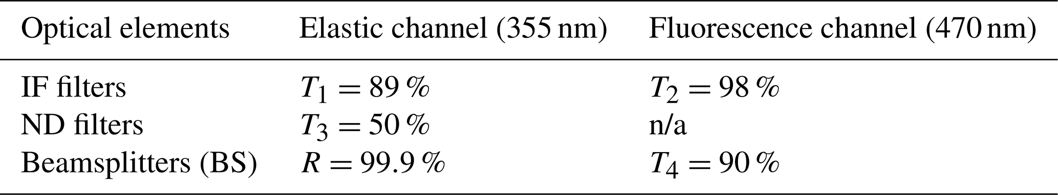
n/a – not applicable.

3.2 Fluorescence spectra clustering/analysis for pollen classification using lidar data

To classify the different taxa of pollen by using the LIF lidar technique we used the Richardson et al. (2019) approach based on their experimental setup, with improvements. The method is based on the spectral decomposition of the LIF lidar signals obtained by a multichannel lidar detector to determine the contribution from each taxon. For this, a database of reference fluorescence spectra (called from now on in vivo data) is obtained for specific pollen types prevailing at Payerne during the study period, including Quercus robur, Dactylis glomerata (proxy for grass pollen), Fagus sylvatica and Betula pendula. Those samples are representative from an optical standpoint for the corresponding genera Quercus, Fagus and Betula and the grass pollen family as shown in Crouzy et al. (2016).

As a second step, we developed a methodology to spectrally decompose the LIF lidar signals obtained by the multichannel lidar detector and retrieve the contributions of the relevant pollen types whose fluorescence signatures are implemented in the detected LIF lidar signals. Thus, to categorise and validate different pollen types we fitted clustering models to represent the pollen spectra during the measured periods. For this, we employed the Spectral Clustering algorithm (Zelnik-Manor and Perona, 2024) which is parametrized by the number of clusters, affinity and the nearest neighbours, while for the scoring function the silhouette scorer was used (Shahapure and Nicholas, 2020). Essentially a silhouette distance is used to measure the quality of the clusters by evaluating how similar an object is to its own cluster compared to other clusters (e.g. Quercus, grass pollen, Fagus and Betula).

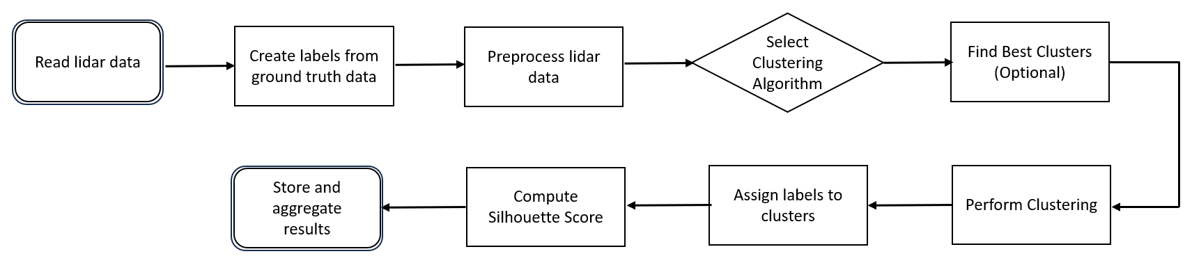
Figure 3 Flowchart of the classification procedure of fluorescence spectra clustering. This procedure is performed for data obtained by the multichannel lidar detector and the in vivo fluorescence spectra.

The silhouette score is calculated from the mean intra cluster distance (in-vitro data) and the mean nearest cluster distance (data obtained by the multichannel lidar detector) for each pollen sample (Shutaywi and Kachouie, 2021). To label our modelled clusters, we employed a similarity search between the in-vitro results and the fitted results. By using the centroids from our models, we computed various distances such as Euclidean, Manhattan, and Minkowski (L3 norm). Our study showed that Spectral Clustering, when paired with Euclidean and Minkowski distances, achieved the highest silhouette scores, resulting in identifying grass pollen as the dominant pollen type, when grouped with Quercus, Betula and Fagus. The procedure is illustrated as a flowchart in Fig. 3.

4 Pollen Climatology of the site

When assessing pollen levels, it is important to understand the thresholds of the exposure classes of allergenic plants (Gehrig et al., 2018; de Weger et al., 2013). These classes are categorized by low, moderate, high, and very high pollen concentrations. Even at low pollen levels, highly sensitive individuals may experience allergic symptoms. Those early manifestations can also be related to local variations of the pollen concentration (e.g., close to sources): pollen is measured at roof level in order to increase mixing and spatial representativity. As pollen concentrations rise, both the number of affected individuals and the intensity of symptoms increase. Since pollen from different plants vary in allergenic potential, the limits for these exposure classes may also differ (Luyten et al., 2024). Figure 4 presents a pollen calendar for the Payerne region showing the distribution of mean pollen concentrations for the 14 most significant allergenic species monitored by MeteoSwiss between 2018 to 2023.

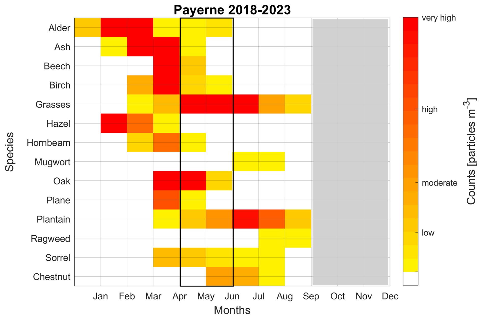
Figure 4 Pollen calendar for various pollen species at the Payerne monitoring station from 2018 to 2023, measured by the Hirst instrument. Gray color indicates periods when the pollen trap was out of service. Yellow, orange, red, dark red colors represent low, moderate, high, and very high pollen concentrations, respectively (adapted from Gehrig et al., 2018).

We see in this figure that the grass pollen load can reach high to very high levels in May and June, with daily average values ranging between 5 to 340 particles m⁻³ in May and from 52 to 270 particles m⁻³ in June (not shown). Moreover, Fagus (Beech) pollen concentration is moderate during May (maximum daily value reaching 57 particles m⁻³), while in June it is found to be very low. Betula (Birch) pollen concentrations still exhibit moderate values during May, (maximum values reaching 15 particles m⁻³), while in June the concentrations decreased to low levels. Finally, Quercus (Oak) pollen presented high values in May (ranging from 0.7 to 106 particles m⁻³) and low levels during June (values ranging from 0.8 to 39 particles m⁻³). It is important to note that the above-mentioned concentration values represent daily averages, the hourly concentration values fluctuate strongly around those averages and reach much higher levels (Chappuis et al., 2020). In the following sections we will present two case studies of bioaerosols profiles obtained during periods of high pollination at ground level and long- and near-range transport of BB particles originating from wildfires in Canada and Germany.

5 Results

5.1 Case 27–29 May 2023

The first case study refers to the period from 27 May (00:00 UTC) to 30 May 2023 (00:00 UTC), when the highest pollen concentrations were measured at ground level, during the PERICLES campaign. The 10 d backward trajectory analysis for the air masses arriving over Payerne at heights over 1.5 km a.s.l. in the period 27–29 May, was obtained by the HYSPLIT model (Fig. S1a, b, c in the Supplement), which confirmed that these air masses originated from wild forest fires (small red dots in Fig. S1a, b, c in the Supplement define the areas where wild forest fires were detected by the MODIS sensor) in North America and Canada, and Germany, and thus, were enriched in BB particles.

Figure 5 illustrates: (panel a) the temporal variation of temperature (T) and relative humidity (RH) obtained at ground level; (panel b) the hourly pollen concentrations obtained by SwisensPoleno (panel c) and Hirst (panel d), as well as the mass concentration of PM₁₀, PM_2.5, NH${}_{\mathrm{4}}^{+}$, NO${}_{\mathrm{3}}^{-}$, SO${}_{\mathrm{4}}^{\mathrm{2}-}$ (panel e) and OC, eBC. During this period, four pollen taxa were observed: grass pollen, Quercus, Betula, and Fagus.

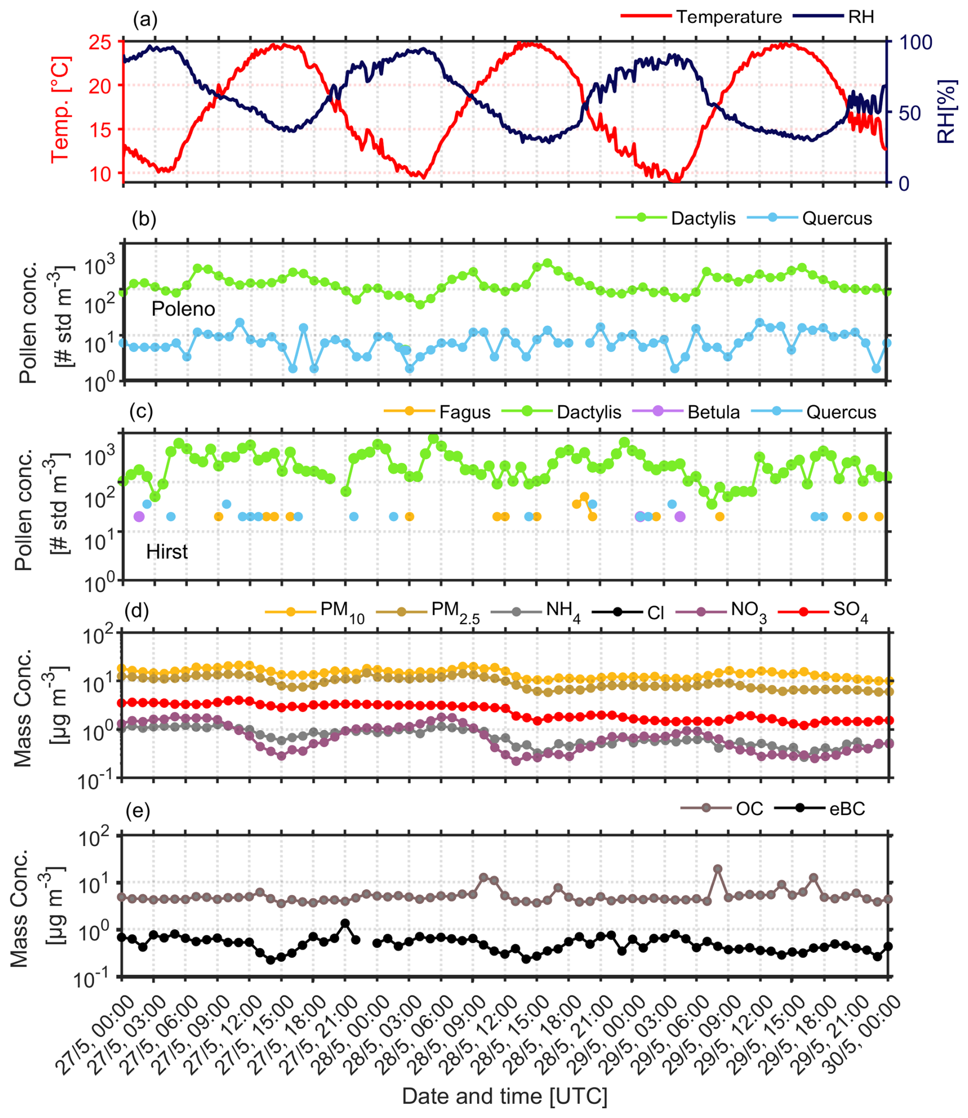
Figure 5 Temporal variability of (a) hourly temperature and RH, pollen concentration obtained by (b) SwisensPoleno (c) Hirst (d) Mass concentration of PM₁₀, PM_2.5, NH${}_{\mathrm{4}}^{+}$, NO${}_{\mathrm{3}}^{-}$, SO${}_{\mathrm{4}}^{\mathrm{2}-}$ and (e) OC, eBC at ground level for the period 27 to 30 May 2023.

It is well documented that grass pollen concentration levels generally peak during daytime (generally higher solar irradiance and temperature levels compared to nighttime) and often tend to increase after rainfall (Kelly et al., 2013; Sabo et al., 2015). In our observations, elevated pollen concentrations were primarily associated with high temperatures and low RH values (Fig. 5a). These observations highlight the connection between meteorological conditions (temperature, RH, precipitation, etc.) and pollen concentration and dispersion, and emphasize the role of meteorological conditions in regulating pollen concentrations near ground (Chappuis et al., 2020). It is evident from Fig. 5b–c that the grass pollen concentrations consistently dominated over the other pollen types, often overpassing values of 10³ particles m⁻³. Specifically, Fig. 5b shows maximum concentration levels of grass pollen of the order of 900–1000 particles m⁻³ (mean value of 315.70 particles m⁻³), while Quercus pollen values showed a maximum of 30 particles m⁻³ (mean value of 11.24 particles m⁻³). Furthermore, Hirst (Fig. 5c) detected a maximum grass pollen concentration of 2340 particles m⁻³, (mean value of 639.63 particles m⁻³). Moreover, the maximum values of Quercus were around 65 particles m⁻³ (mean value of 6.76 particles m⁻³). We must note here that the mean values of Quercus concentrations measured by SwisensPoleno (11.24 particles m⁻³) and Hirst (6.76 particles m⁻³), are quite close, although the maximum values measured by Hirst are significantly higher than those measured by SwisensPoleno. Hirst also measured Betula pollen with maximum concentrations of the order of 33 particles m⁻³ (mean value of 1.02 particles m⁻³), while the Fagus concentrations showed a maximum value of 98 particles m⁻³ (mean value of 7.46 particles m⁻³). Betula and Fagus pollen were not detected by the SwisensPoleno, which could be related to the postprocessing applied to avoid false positive detections close to detection threshold. The SwisensPoleno was not able to achieve a sufficient number of precise detections for the label to be activated (Crouzy et al., 2022).

Furthermore, in Fig. 5d we present the temporal variability of the mass concentration of PM₁₀, PM_2.5, NH${}_{\mathrm{4}}^{+}$, NO${}_{\mathrm{3}}^{-}$, SO${}_{\mathrm{4}}^{\mathrm{2}-}$ and of OC, eBC (Fig. 5e) for the period 27 to 30 May 2023. The PM₁₀ levels varied from 1.9 to 34.7 µg m⁻³, with an average concentration of 12.162 µg m⁻³. For PM_2.5, the minimum recorded value was 0.80 µg m⁻³, reaching up to 18 µg m⁻³, and an average of 8.30 µg m⁻³. NH${}_{\mathrm{4}}^{+}$ levels ranged between 0.20 and 2.67 µg m⁻³, with a mean value of 0.86 µg m⁻³, typical of ambient concentrations due to agricultural activities in Payerne. Moreover, NO${}_{\mathrm{3}}^{-}$ concentrations ranged from 0.17 to 6.08 µg m⁻³, with an average value of 1.16 µg m⁻³. Finally, SO${}_{\mathrm{4}}^{\mathrm{2}-}$ concentration levels ranged between 0.96 to 4.71 µg m⁻³, with a mean value 2.53 µg m⁻³. Additionally, the concentration of SO${}_{\mathrm{4}}^{\mathrm{2}-}$ is influenced by both local and regional emissions (Gautam et al., 2023), however, the mean concentrations over Payerne remain quite low (Hueglin et al., 2024).

Figure 5e, shows the temporal variation of hourly averaged values of OC and eBC and concentrations measured by the ToF-ACSM and the Aethalometer AE-33, respectively. The OC concentrations generally remained low (background values) and ranged between 3–8 µg m⁻³ throughout the measurement period, with morning peaks greater than 10 µg m⁻³ on 28 May (12.5 µg m⁻³ at 10:00–11:00 UTC) and 29 May (19 µg m⁻³ at 08:00 UTC and 12 µg m⁻³ at 17:00 UTC) indicating the presence of organic particles at ground level. In contrast, eBC concentrations remained below 1 µg m⁻³ and varied from 0.22 µg m⁻³ to a maximum value of 1.34 µg m⁻³ on 27 May at 21:00 UTC, showing no presence of BB particles at ground level.

Figure 6a–c present the spatio-temporal evolution of the range-corrected lidar signal (RCS) at the fluorescence channel (470 nm), while Fig. 6d–f present the vertical profiles of the aerosol backscatter b₃₅₅ and fluorescence backscatter b_F coefficients and the fluorescence capacity G_F. The vertical profiles of the relative humidity (RH) and potential temperature (θ) obtained by local radiosoundings at 23:00 UTC on the nights of 27–29 May 2023 are presented in Fig. 6g–i.

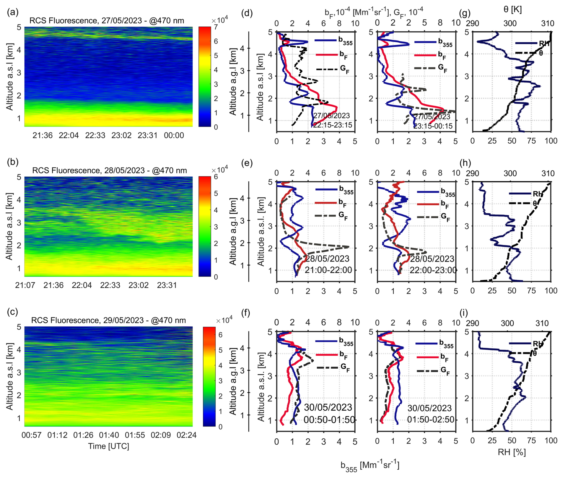
Figure 6 (a–c) Spatio-temporal evolution of the range-corrected lidar signal (RCS) at the fluorescence channel (470 nm) (d–f) aerosol b₃₅₅ and fluorescence b_F backscatter coefficients and G_F profiles (hourly means, with times indicated in the plots) (g–i) RH and θ as obtained by radiosonde launches around 23:00 UTC for the period 27–29 May 2023.

We note in Fig. 6a (27 May) the presence of distinct nearly homogeneous aerosol layers present at the fluorescence channel (yellow and green filaments) from ground up to about 1.85 km a.s.l. height (top of the PBL as derived by local radiosounding data, cf. Fig. 6g), while a thinner aerosol layer was observed between 4.7–4.9 km. Based on the back trajectory analysis of the air masses arriving over Payerne (at 23:00 UTC, as shown in Fig. S1a) we found that the distinct aerosol layer observed around 4.8 km was related to smoke particles released by intensive forest fires in Canada and transported over the Atlantic ocean to Switzerland. The lower yellow-green layer below 1.8 km was confined inside the PBL during the whole night. The fluorescence particles inside the PBL showed an increased fluorescence backscatter ($b_{\mathrm{F}}\sim \mathrm{7.4}\times {\mathrm{10}}^{-\mathrm{4}}$ Mm⁻¹ sr⁻¹) and a well-mixed elastic backscatter coefficient ($b_{\mathrm{355}}\sim \mathrm{2.2}\times {\mathrm{10}}^{-\mathrm{4}}$ Mm⁻¹ sr⁻¹) up to 1.8 km height (Fig. 6d). Indeed, referring to Fig. 5b, c we observed increased values of grass pollen (>100 particles m⁻³) at ground level during that night, which explains the high values of b_F between 22:15 UTC (27 May) and 00:15 UTC (28 May) probably due to mixed bioaerosols (BB and pollen) and moderate fluorescence capacity indicating the presence of fluorescence particles inside the PBL. Between 2–3 km, a thin aerosol layer was identified (Fig. 6a) with moderate b₃₅₅ (1.6 Mm⁻¹ sr⁻¹) and still strong b_F ($<\mathrm{5}\times {\mathrm{10}}^{-\mathrm{4}}$ Mm⁻¹ sr⁻¹) and increased G_F (1.5–3.25 × 10⁻⁴) values, confirming again the presence of fluorescent aerosols (Hu et al., 2022; Veselovskii et al., 2022a). Within this layer, the RH increases with height (from 63 % to over 85 %), while θ shows a slight increase (300 to 303 K), indicating the presence of a stable layer (cf. Fig. 6g). The thin aerosol layer around 4.5 km (Fig. 6d) exhibited increased elastic backscatter (b₃₅₅∼1.9 Mm⁻¹ sr⁻¹) but with a lower fluorescence backscatter ($b_{\mathrm{F}}\sim \mathrm{1.4}\times {\mathrm{10}}^{-\mathrm{4}}$ Mm⁻¹ sr⁻¹) coefficient, indicating fewer fluorescence aerosols due to long-range transport of dried BB aerosols (Reichardt et al., 2025), as the RH decreased down to ∼ 8 %.

On the following day 28 May, aerosols are more dispersed above the PBL (located ∼ 2 km a.s.l.), with a ∼ 1.8 km thick aerosol layer extending from 2.2 to 4.0 km (Fig. 6b). The aerosols inside a quite well-mixed PBL, exhibited similar trends as during the previous night, with slightly lower b₃₅₅ values (b₃₅₅∼1.4 Mm⁻¹ sr⁻¹), but still with quite high b_F values ($b_{\mathrm{F}}\sim \mathrm{3.8}\times {\mathrm{10}}^{-\mathrm{4}}$ Mm⁻¹ sr⁻¹) and notably increased G_F values ($G_{\mathrm{F}}\sim \mathrm{4}\times {\mathrm{10}}^{-\mathrm{4}}$) at the top of the PBL, indicative of the presence of fluorescent aerosols (Hu et al., 2022; Veselovskii et al., 2022a, b) inside the PBL (Fig. 6e, h), linked again to high pollen concentrations of grass pollen (> 100 particles m⁻³) (Fig. 5b, c) at ground. In the aerosol layer between 2.0–3.5 km (Fig. 6e between 22:00–23:00 UTC), b₃₅₅ increased to 1.6–2.0 Mm⁻¹ sr⁻¹, while b_F and G_F decreased to $\mathrm{2.3}\times {\mathrm{10}}^{-\mathrm{4}}$ Mm⁻¹ sr⁻¹ and $\mathrm{1.1}\times {\mathrm{10}}^{-\mathrm{4}}$, respectively, showing a weaker fluorescence signal than inside the PBL, probably due to mixed BB with continental polluted aerosols. The RH values increased inside that layer (from 24 % to 52 %), while θ seem to be constant (Fig. 6h). Between 3.5–5.0 km, we observed a similar pattern as in the second aerosol layer regarding the optical properties, while the RH seem to be stable at around 14 % and θ slightly increases from 305 to 308 K (Fig. 6h) in this stable layer. As on the previous day, the air masses arriving between 2.0 and 5.0 km height are related to long-range transport of BB aerosols, showing intense fluorescence (Reichardt et al., 2025).

On 29 May, the spatio-temporal evolution of the RCS signals at 470 nm, shows a quite well-mixed fluorescence layer from 1.5 to 3.5 km height ($b_{\mathrm{F}}\sim \mathrm{2}\times {\mathrm{10}}^{-\mathrm{4}}$ Mm⁻¹ sr⁻¹), with increased b_F values ($b_{\mathrm{F}}\sim \mathrm{3}\times {\mathrm{10}}^{-\mathrm{4}}$ Mm⁻¹ sr⁻¹) over 3.5 km (Fig. 6c). On that day the PBL height was confined below 1.2 km, where a distinct thin fluorescence layer is observed (Fig. 6c) with $b_{\mathrm{F}}\sim \mathrm{1.5}\times {\mathrm{10}}^{-\mathrm{4}}$ Mm⁻¹ sr⁻¹ during the first observation period (00:50–01:50 UTC), with similar value in the next hour (01:50–02:50 UTC) (Fig. 6i). This is again linked to the presence of fluorescent pollen aerosols of grass pollen (>100 particles m⁻³) at ground as shown in Fig. 5b, c. In the free troposphere just above the PBL (∼ 1.5 km height) a second thin fluorescence layer (∼ 2 km height) is observed (Fig. 6c). Meanwhile, the G_F values show a nearly constant profile from the top of the PBL to ∼ 3.5 km (G_F ∼ 2.7 × 10⁻⁴ between 00:50–01:50 UTC (Fig. 6f) and G_F ∼ 1.5 × 10⁻⁴ between 01:50–02:50 UTC (Fig. 6i)), with enhanced G_F values between 3.5 and 4.5 km (3.0–4.2 × 10⁻⁴) between 00:50–01:50 UTC (Fig. 6e, f) and ∼ 2.8 × 10⁻⁴ (01:50–02:50 UTC). We observe that the RH (Fig. 6i) varied slowly from 68 % to 47 % (2.0–4.0 km height), with relatively stable aerosol optical properties (b_aer, G_F, b_F), within a stable atmospheric layer (θ ranged from 300 to 306 K) (Fig. 6i). These observations during May, highlighted the presence of fresh (<2 d) and aged (>5 d) fluorescence BB particles in the altitude region 1.5–5.0 km a.s.l. heigh over Payerne, transported from the wildfires in Germany and Canada, respectively (Fig. S1a, b, c).

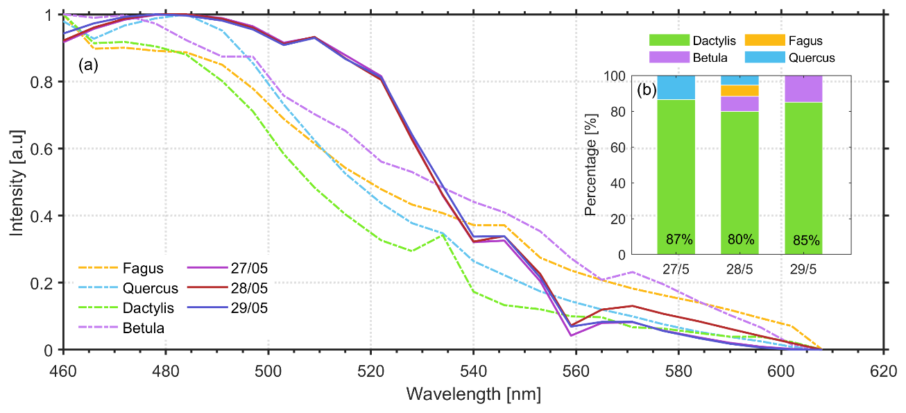
Figure 7 (a) Pollen fluorescence spectra of Fagus, Quercus, Dactylis and Betula obtained in vivo by lidar excitation at 355 nm (dashed lines) and pollen spectra (continuous lines) obtained by the lidar multichannel spectrometer, along with the (b) percentages of each pollen type for various clustering algorithms and metrics (from 27–29 May 2023) from ground up to 1.2 km a.s.l.

As a next step we spectrally decompose the fluorescence spectra obtained by the lidar multichannel spectrometer over 1 h period and averaged in the height region from ground up to 1.2 km a.s.l. (Fig. 7a) into the pollen types measured at ground level by SwisensPoleno and the Hirst trap, to examine the feasibility of the lidar multichannel spectrometer LIF technique to retrieve and categorise the different pollen types aloft. The validation of our methodology will refer to the ground pollen data with increased concentrations during the observation period from 27 to 29 May, Fagus, Betula and Quercus, with the grass pollen being the dominating pollen taxa (Fig. 5b, c). To this end, at first Fig. 7a presents the in vivo LIF fluorescence spectra (dashed lines) of four different pollen types (Dactylis glomerata (proxy for grass pollen), Fagus sylvatica, Betula pendula and Quercus robur) obtained by laser excitation at 355 nm under laboratory conditions (Richardson et al., 2019). Additionally, in the same figure we present the fluorescence spectra measured by the lidar multichannel spectrometer during the observation period from 27 to 29 May, averaged in the height region from ground up to 1.2 km a.s.l. height (continuous lines). Then, we followed the methodology explained in Sect. 3.2 applied to lidar multichannel spectrometer signals and the corresponding in vivo spectra of these selected pollen types. In Fig. 7b we quantify the presence of each pollen type aloft as a percentage of pollen counts for each day of the observed period. On 27 May, grass pollen was the most prevalent pollen type in the atmosphere, contributing to ∼ 87 % in the lidar multichannel spectrometer signal, while Quercus accounted for ∼ 13 %. These results are in accordance with the in situ data obtained from SwisensPoleno and Hirst (Fig. S2), where grass pollen represented 97 % and Quercus accounted for 3 %. On 28 May, the presence of grass pollen reached 80 %, with Betula, Fagus and Quercus reaching 8 %, 6 % and 5 %, respectively. In this case, the in situ data similarly indicated an increased percentage of grass pollen at approximately 95 %, with Quercus and Fagus contributing 4 % and 1 %, respectively, while Fagus concentrations were generally low or absent. On 29 May, the algorithm detected both grass pollen reaching a peak of 85 %, and Betula at 15 % (Fig. 7b), in accordance with the Hirst and SwisensPoleno data (see also Fig. 4), which indicated high concentration (∼ 250–300 particles m⁻³ at 23:00 UTC) of grass pollen along with a small presence of Quercus (∼ 10 particles m⁻³) concentrations, while Betula was absent at that day.

5.2 Case 12–15 June 2023

Figure 8a presents the daily evolution of temperature and RH at ground level. The pattern observed during the first case study (27–29 May 2023) is evident here as well, with increased pollen concentrations coinciding with the highest temperature and lowest RH values. Regarding the temporal variations of the hourly pollen concentrations measured at ground level, the SwisensPoleno did not detect any pollen concentration of Betula, Quercus and Fagus as during May 2023, while grass pollen was recorded at a maximum concentration of 644 particles m⁻³ and a mean one of 159.81 particles m⁻³ (Fig. 8b). Hirst measured a mean concentration of grass pollen equal to 196.47 particles m⁻³ with a maximum of 878 particles m⁻³, while Quercus, Fagus and Betula showed very low concentrations (around 15 particles m⁻³) (Fig. 8c). Furthermore, the PM₁₀ levels varied from 7.6 to 23.3 µg m⁻³, with an average concentration of 15.6 µg m⁻³. For PM_2.5, the minimum recorded value was 5.5 µg m⁻³, reaching up to 13.1 µg m⁻³, and an average of 7.40 µg m⁻³. (Fig. 8d). Moreover, the OC concentrations generally ranged between 2.33–5.40 µg m⁻³, while the eBC ones were again very low with values ranging from 0.08 to 1.25 µg m⁻³ (Fig. 8e), indicating the absence of BB aerosols.

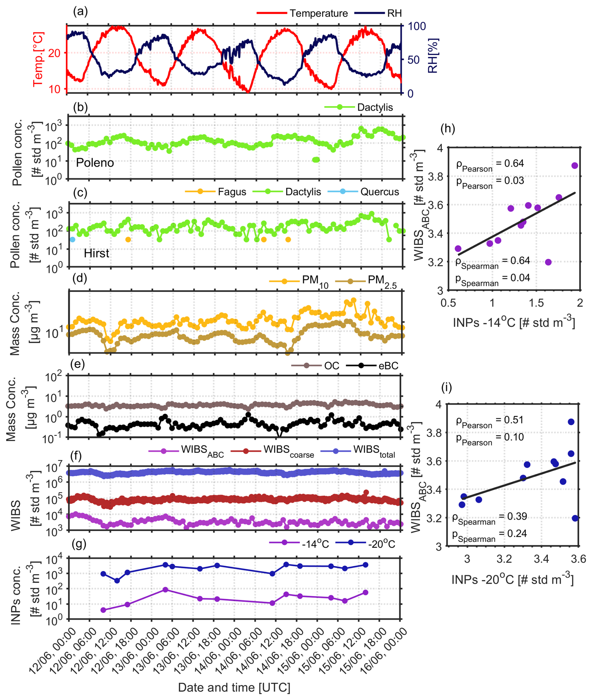
Figure 8 (a) Temporal evolution of daily temperature and RH from MeteoSwiss data, as well as, evolution of the hourly pollen concentration obtained by (b) SwisensPoleno (c) Hirst (d) Mass concentration of PM₁₀, PM_2.5, and (e) OC, eBC at ground level, (f) WIBS_ABC, WIBS_coarse, and WIBS_total particle number concentrations (g) INP concentrations at −14, −15 and −20 °C, and the correlations between (h) INPs at −14 °C and WIBS_ABC (i) INPs at −20 °C and WIBS_ABC for the period between 12 and 15 June 2023.

Figure 8f shows the number concentrations of bioaerosols measured at the WIBS_total, WIBS_coarse, and WIBS_ABC channels. The WIBS_ABC channel measured concentrations between 1000 and 10 000 particles cm⁻³, which is at least two orders of magnitude higher than the pollen number concentrations shown in Fig. 8b to c. This is because the WIBS_ABC channel refers to the presence of a wide range of fluorescent biological particles, including pollen particles. Daily minimum WIBS_ABC number concentrations tend to appear in the morning hours, whereas maximum values show up after midnight, more specifically on 12 to 14 June (Fig. 8f). Figure 8g presents the INP number concentrations at −14 and −20 °C.

The INP concentrations at −20 °C are higher than those at −14 °C by more than one order of magnitude. To investigate the sources of INPs, we compared the correlations between the INP number concentrations and the WIBS_total, WIBS_coarse, and WIBS_ABC ones, as well as the total pollen number concentrations measured by the SwissensPoleno, and Hirst, and the mass concentrations of eBC and OC. We found that the INPs activated at −14 and −20 °C show insignificant correlations with OC (Fig. S3a, b) and eBC (Fig. S3c, d), thus, suggesting a relative unimportant role of BB particles on mixed-phase cloud formation (Gao et al., 2025; Kanji et al., 2020). In contrast, the WIBS_total and INPs are positively correlated, but with a low correlation coefficient (Fig. S4a, b). This may be due to a minor fraction of INPs in the total number of aerosol particles (Fig. 8f, g). More precisely, the INPs at −14 °C have significant correlations with WIBS_ABC particles (Fig. 8h), two of which show ρ_Pearson=0.64 (p_pearson=0.03) and ρ_Spearman=0.64 (p_Spearman=0.04). This indicates the important contribution of FBAPs in INPs activated at −14 °C. However, the correlation analysis shows that the detected pollen particle number concentrations from SwisensPoleno (Fig. S5a) and Hirst (Fig. S5c) are insignificantly correlated with INPs at −14 °C. This may indicate that not all types of pollen particles are active INPs and the INPs originated from FBAPs may include a broad range of biological particles in addition to pollen (Gao et al., 2024; Kanji et al., 2017; Morris et al., 2013). In addition, the INPs at −20 °C are correlated with WIBS_coarse particles (Fig. S4c, d), by showing ρ_Pearson=0.72 (p_pearson=0.01) and ρ_Spearman=0.52 (p_Spearman=0.10), which suggests coarse-sized particles, such as soil dust, pollen and large-sized fungal spores, contribute to the observed INPs at −20 °C. The above results are consistent with similar finding presented in the literature and confirm that the biological particles are more relevant INPs for $T>-\mathrm{15}$ °C, while dust particles generally contribute cloud ice formation for $T<-\mathrm{15}$ °C (Murray et al., 2012).

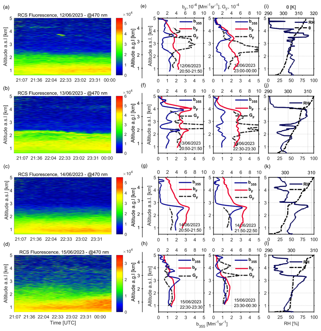
Figure 9 (a–d) Spatio-temporal evolution of the range-corrected lidar signal (RCS) at the fluorescence channel (470 nm) (e–h) aerosol b₃₅₅ and fluorescence b_F backscatter coefficients and G_F profiles (hourly means, with times indicated in the plots) (i–l) RH and θ as obtained by radiosonde launches around 23:00 UTC for the period 12–15 June 2023.

Figure 9a–d present the spatio-temporal evolution of the range-corrected lidar signal (RCS) at the fluorescence channel (470 nm), while Fig. 9e–h present the vertical profiles of b₃₅₅, b_F and G_F. The vertical profiles of RH and θ obtained by local radiosondings at 23:00 UTC on the nights 12–15 June 2023, are presented in Fig. 9i–l. The general overview of Fig. 9a–d shows the presence of aerosol fluorescent layers from ground up to 2–2.5 km heigh, which at near ground level (below 1.2–1.5 km) may be influenced mainly by the high concentrations of grass pollen from local sources, as discussed in Fig. 8b, c. The backward trajectory analysis of the air masses arriving over Payerne between 1.5–4.0 km during the nights of 12–15 June indicated as aerosol source region the wildfires occurring in Germany (Fig. S9a, b, c, d).

More specifically, on 12 June nearly homogeneous aerosol RCS signals at the fluorescence channel are observed inside the PBL (from ground up to 1.8 km) (Fig. 9a), as also shown in Fig. 9e on the same heights, at the vertical profiles of b₃₅₅, b_F and G_F. This homogeneous layer is characterized by b_F values ranging between $\mathrm{4.5}\times {\mathrm{10}}^{-\mathrm{4}}$ Mm⁻¹ sr⁻¹ (20:50–21:50 UTC) and $\mathrm{5.2}\times {\mathrm{10}}^{-\mathrm{4}}$ Mm⁻¹ sr⁻¹ (23:00–00:00 UTC), and G_F ones between $\mathrm{3.2}\times {\mathrm{10}}^{-\mathrm{4}}$ (20:50–21:50 UTC) and $\mathrm{4.5}\times {\mathrm{10}}^{-\mathrm{4}}$ (23:00–00:00 UTC). The vertical profile of b₃₅₅ in the same layer shows moderate values of the order of 1.4 Mm⁻¹ sr⁻¹ during that night (Fig. 9e). The RH values are close to 50 % up to 1.8 km height indicating a nearly well-mixed and stable ($\mathrm{d}\mathit{\theta }/\mathrm{d}z>\mathrm{0}$) PBL layer. At heights from 2.5 to 3.5 km, where again similar stable meteorological conditions prevail (atmospheric stability, since $\mathrm{d}\mathit{\theta }/\mathrm{d}z>\mathrm{0}$) and RH∼ 40 %–50 %), the G_F shows increased values of $\mathrm{7.3}\times {\mathrm{10}}^{-\mathrm{4}}$ (20:50–21:50 UTC) and even up to 10⁻⁵ (23:00–00:00 UTC), while the b₃₅₅ (∼ 1.0 Mm⁻¹ sr⁻¹) and b_F (∼ $\mathrm{3}\times {\mathrm{10}}^{-\mathrm{4}}$ Mm⁻¹ sr⁻¹) profiles show nearly constant values during that night. At the top (at 3.5 km) of this 1 km thick atmospheric layer very humid air masses are observed (RH ∼ 85 %) giving rise to a local peak of b₃₅₅ indicating a possible particle hygroscopic growth (Miri et al., 2024; Navas-Guzmán et al., 2019). Over 3.5 km height thin filaments of smoke particles are observed around 3.8 and 4.4 km (Fig. 9a), while the relevant b₃₅₅ and b_F profiles present decreasing trends (Fig. 9e).

On 13 June, again nearly homogeneous aerosol RCS signals at the fluorescence channel were observed inside the PBL (from ground up to 1.8 km) (Fig. 9b) with a fluorescing smoke filament observed at 2.2 km. The b_F profile is nearly constant ($b_{\mathrm{F}}\sim \mathrm{4.2}\times {\mathrm{10}}^{-\mathrm{4}}$ Mm⁻¹ sr⁻¹) with height up to 3.8 km, except between 1.5 and 2.2 km where it presents a local maximum of 4.2–6.2 Mm⁻¹ sr⁻¹ (20:50–21:50 UTC). Later that night (23:00–23:30 UTC) it becomes nearly constant (∼ 4.5–5.0 Mm⁻¹ sr⁻¹) with height from ground up to 3.8 km (Fig. 9f). The G_F profiles are nearly homogeneous up to 3.8 km, except the height region between 2.2–2.5 up to 2.9 km where they show pronounced maxima due to very low b_F values. The profile of $\mathrm{d}\mathit{\theta }/\mathrm{d}z>\mathrm{0}$ remains positive, indicating stable meteorological conditions up to 3.8 km.

On 14 June, again nearly homogeneous aerosol RCS signals at the fluorescence channel were observed inside the PBL (from ground up to 1.9 km) with decreasing values up to 2–2.7 km (Fig. 9c). The vertical profiles of b₃₅₅ (mean value $\mathrm{2.0}\times {\mathrm{10}}^{-\mathrm{4}}$ Mm⁻¹ sr⁻¹) and b_F (mean value $\mathrm{6}\times {\mathrm{10}}^{-\mathrm{4}}$ Mm⁻¹ sr⁻¹) show a well-mixed layer up to 1.9–2.0 km height with increasing values up to 2.7 km. The G_F profiles (mean values of $\mathrm{3}\times {\mathrm{10}}^{-\mathrm{4}}$) are nearly constant up to 2.0 km with slightly decreasing values up to 2.7 km. Over that height the b₃₅₅ and b_F profiles show decreasing values indicative of the presence of low aerosol concentrations (Fig. 9g). In Fig. 9k we note the presence of a humid layer (60 % < RH < 85 %) between 2.0–3.0 km which leads to an increase of b₃₅₅ and b_F values around 2.7 km possibly due to hygroscopicity growth and enhanced fluorescence, respectively (Miri et al., 2024).

On 15 June, more intense than last days' aerosol RCS signals at the fluorescence channel were observed, below 1.6 km, especially during the late evening hours (23:30–00:30 UTC), with decreasing intensity up to ∼ 2.5 km (Fig. 9d). From 22:30 to 23:30 UTC the vertical profile of b₃₅₅ (mean value $\mathrm{1.2}\times {\mathrm{10}}^{-\mathrm{4}}$ Mm⁻¹ sr⁻¹) is homogeneously distributed up to 2.2 km with increasing values up to 3.0 km (due to the presence of a humid layer with RH of 85 %) and then decreasing values up to 5 km. The b_F profile (mean value 3.5 × 10⁻⁴ Mm⁻¹ sr⁻¹) shows a very well-mixed layer from ground up to 3.0 km height, with decreasing values at higher altitudes. The G_F profile is nearly constant up to 2.3 km (mean values ∼ 2.9 × 10⁻⁴) and decreases up to 5 km. Similar behavior show the vertical profiles of b_F and G_F from ground up to 3.1 km, in the period 23:30–00:30 UTC except the b₃₅₅ profile which remains continuously well distributed below that height. On this day the decreasing values of the b₃₅₅, b_F and G_F profiles over 3.1 km height are indicative of the presence of low bioaerosol concentrations.

Overall, in most studied cases in June, we found that the enhanced values of b₃₅₅ and b_F below 2–3 km down to 1.5 km are linked to increased fluorescence backscatter attributed to BB particles originating from wildfires in Germany. However, the enhanced values of the aerosol RCS signals at the fluorescence channel below 1.5 km are due to the presence of high concentrations of grass pollen as also found near ground (Fig. 8b, c).

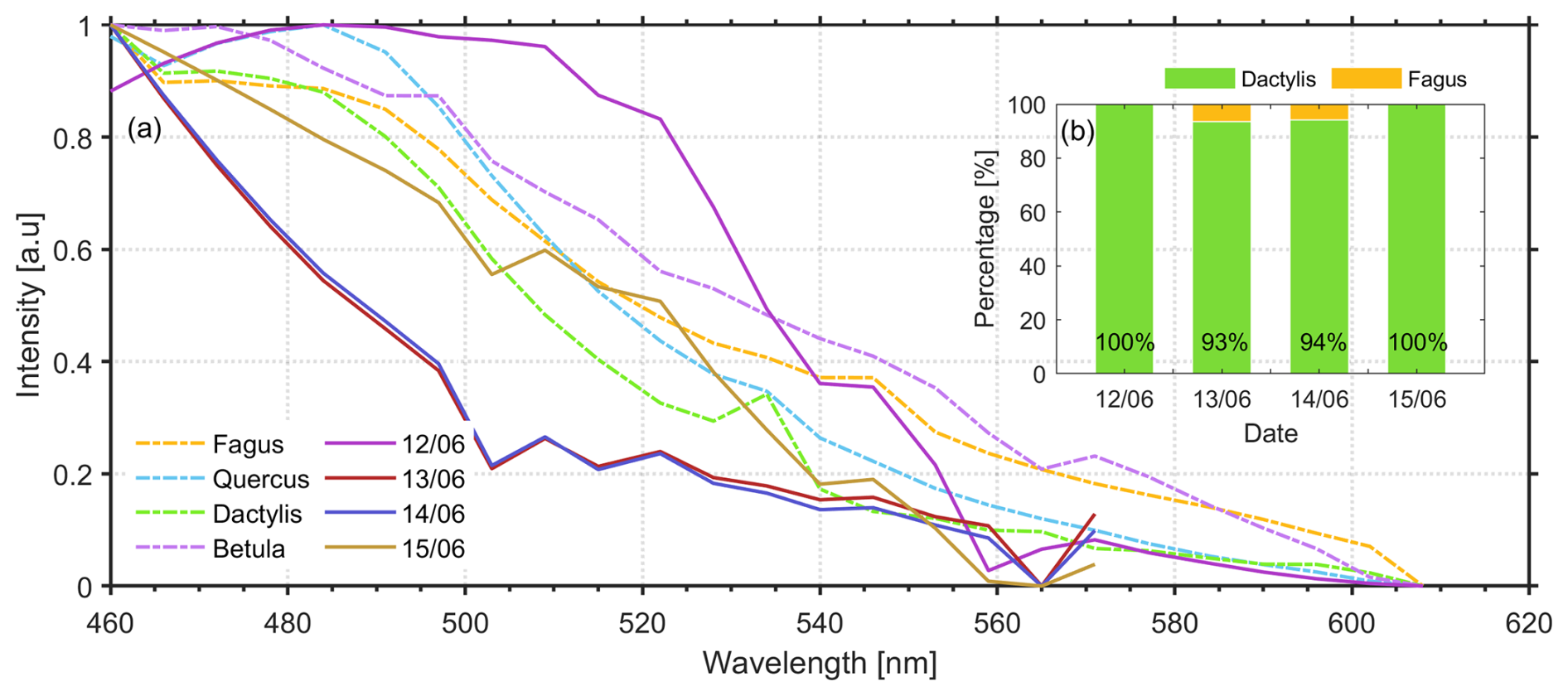
Figure 10 (a) Pollen fluorescence spectra of Fagus, Quercus, Dactylis and Betula obtained in vivo by lidar excitation at 355 nm (dashed lines) and pollen spectra (continuous lines) obtained by the lidar multichannel spectrometer, along with (b) the percentages of each pollen type for various clustering algorithms and metrics (from 12–15 June 2023) from ground up to 1.2 km a.s.l.

As in the previous case study, we spectrally decompose the fluorescence spectra obtained by the lidar multichannel spectrometer over 1 h period and averaged in the height region from ground up to 1.2 km a.s.l. for the period 12–15 June (Fig. 10a) into the pollen types measured at ground level by SwisensPoleno and the Hirst trap, to retrieve and categorise the different pollen types aloft.

Figure 10a presents the in vivo LIF fluorescence spectra (dashed lines) of four different pollen types Dactylis glomerata, Fagus sylvatica, Betula pendula and Quercus robur obtained by laser excitation at 355 nm under laboratory conditions as explained in the previous case of May 2023. Additionally, in the same figure we present the fluorescence spectra obtained by the lidar multichannel spectrometer from 12 to 15 June, averaged in the height region from ground up to 1.2 km a.s.l. height (continuous lines).

In Fig. 10b we quantify the presence of each pollen type aloft as a percentage for each day of the observed period. Based on our algorithm, we observed that on most days, grass pollen was the only pollen type detected. For instance, on 12 June, grass pollen showed a 100 % presence, while on 13 and 14 June, Fagus sylvatica was also detected, though only with 7 % and 6 % presence, respectively. On 15 June, grass pollen once again dominated with 100 % presence in the atmosphere. These results are in good agreement with the in situ pollen measurements from SwisensPoleno and Hirst (Fig. S7), confirming that grass pollen was the most dominant pollen type in the atmosphere. Regarding the in situ measurements (Fig. S7), grass pollen again showed the highest concentrations along all days, with peaks around 79 % on 12 and 14 June. Betula exhibited moderate concentrations, reaching highest percentages of ∼ 33 % on 15 June. This is probably related to the uncertainties of the method, as birch trees are not typically flowering during that period. Quercus and Fagus showed very low or zero concentrations, with Quercus peaking at around 7 % on 13 June, while Fagus presence remaining absent throughout the period. The in situ data highlight again the predominance of grass pollen over a noticeable presence of Betula and near-zero concentrations of all other pollen types. Note that differences between the in-vivo and the lidar spectra can result from the contribution of other fluorescing particles or other grass pollen species. The absence of a tail in longer wavelengths however suggests a dominant contribution of grass pollen.

5.3 Impact of air mass transport on fluorescence

In the two-case studies analyzed in the preceding sections we focused on the detection of bioparticles in the first 5 km a.s.l. and found that from near ground to ∼ 1.0–1.5 km height, pollen particles dominate, while over 1.8–2.0 km smoke layers or distinct filaments of BB particles are observed. The smoke particles were found to originate from long- and/or near-range wild forest fires in Canada and Germany that occurred during May and June 2023 (Figs. S1 and S6, respectively). In this section we will examine how the aging of the smoke particles from the Canadian forest fires affects the b_F values aloft, embedded in the same air masses overpassing a central European lidar station (at heights below 8 km) before reaching Payerne. To this end we will use published data of b_F from the literature at 532 nm from Lindenberg, Germany (DWD), (Reichardt et al., 2025), and Payerne, Switzerland (PAY) (this study) from 26 to 29 May 2023.

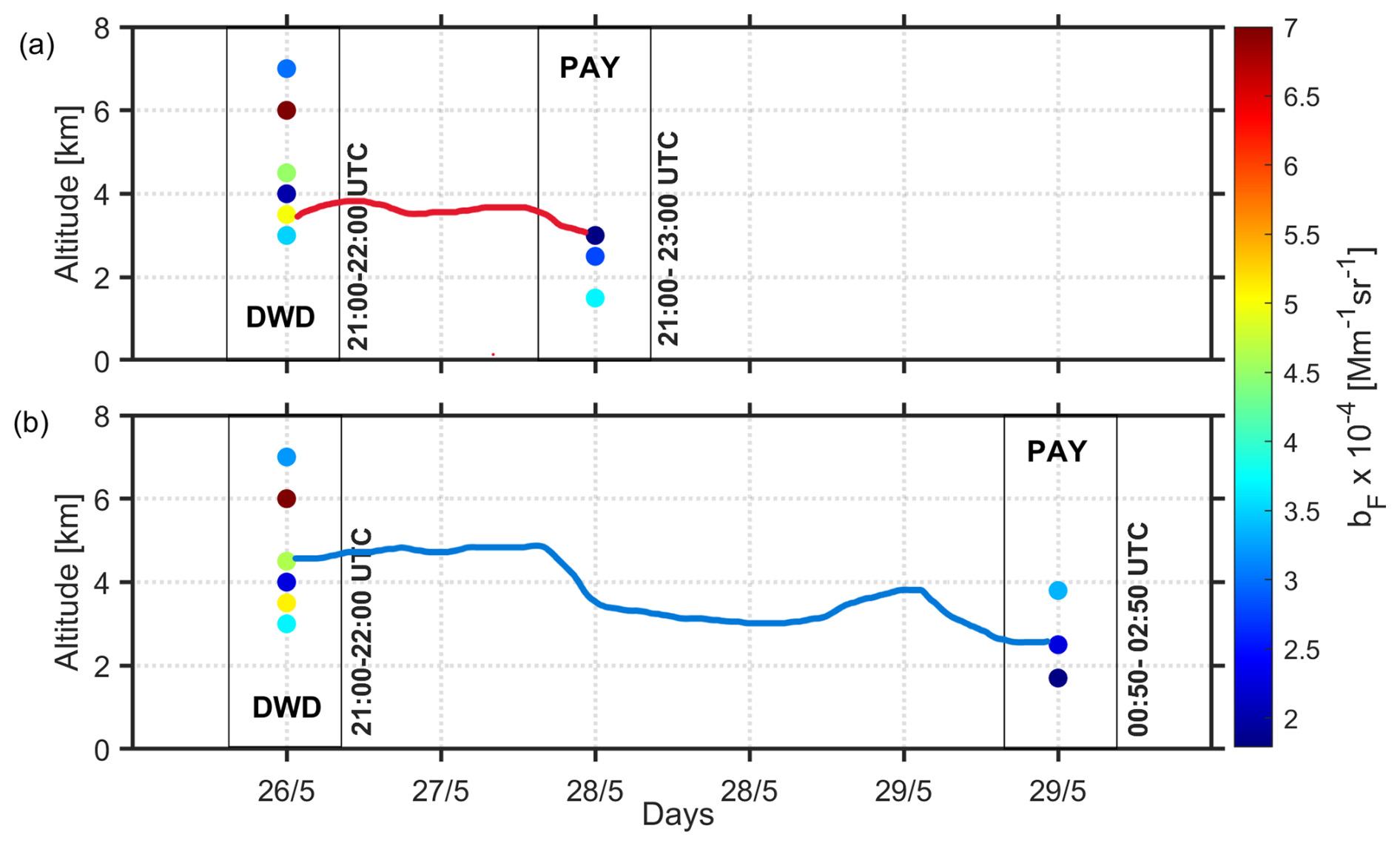
Figure 11 Temporal and vertical variations of b_F measured over two stations (DWD and PAY) between 1.8 and 8 km height, during the BB aerosols from wild forest fires from (a) long-range transport from Canada (26 to 28 May 2023) (b) near-range transport from Germany (26 to 29 May 2023). The observing time periods are indicated also for each station.

Figure 11a shows the b_F profiles over DWD (26 May, 21:00–22:00 UTC) and PAY (28 May, 21:00–23:00 UTC). In this figure we show with red line the air mass trajectories which overpassed the DWD station at 3.5 km (26 May, 21:00–22:00 UTC), then arrived two days later over PAY (28 May, 21:00–23:00 UTC) at around 3.0 km height. Along this trajectory the b_F starting over DWD at 3.5 km presented quite high values (∼ 5.0 × 10⁻⁴ Mm⁻¹ sr⁻¹), but during their descent to lower heights (3.0 km) on the following days (27–28 May) they were characterized by lower values by a factor ∼ 3 (∼ 1.8 × 10⁻⁴ Mm⁻¹ sr⁻¹) indicating smoke aerosols with lower fluorescence potential, probably due to mixing with non-fluorescent (e.g. continental polluted) aerosols of different RH values at lower heights. Similar behavior showed the air masses (blue line) in Fig. 11b, starting at 4.5 km over DWD (26 May, 21:00–22:00 UTC), reached PAY on 30 May (00:50–02:50 UTC) at 2.5 km. Along this transport the b_F values passed from ∼ 4.5 × 10⁻⁴ to 2.0 × 10⁻⁴ Mm⁻¹ sr⁻¹, now showing a ∼ 50 % reduction on the b_F values, indicating again a possible mixing of BB aerosols of lower concentrations with non-fluorescent (e.g. continental polluted) aerosols of different hygroscopicity values at lower heights.

6 Conclusions

This study demonstrated the potential of an advanced LIF lidar approach, combining single-channel fluorescence detection with a 32-channel spectrometer, to characterize both pollen and biomass burning aerosols from the surface up to 5 km during the PERICLES campaign in spring–summer 2023 in Payerne, Switzerland. Building upon the experimental setups implemented by Richardson et al. (2019) and Veselovskii et al. (2021), this technique offered, for the first time in this region, the capability to discriminate pollen taxa aloft and to distinguish fresh from aged smoke layers with high temporal and vertical resolution. Compared to traditional ground-based methods such as Hirst, SwisensPoleno, or WIBS, the LIF lidar enabled the continuous monitoring of the spatio-temporal evolution of bioaerosols and smoke in the free troposphere, while also allowing quantitative comparisons with in situ measurements. Ground-based pollen data (Quercus, grass pollen, Fagus, and Betula) collected with Hirst and SwisensPoleno samplers were used to validate the lidar-derived pollen fractions, whereas air pollution measurements (PM₁₀, PM_2.5, NH${}_{\mathrm{4}}^{+}$, Cl⁻, NO${}_{\mathrm{3}}^{-}$, SO${}_{\mathrm{4}}^{-\mathrm{2}}$, eBC, OC) provided information on the influence of biomass burning aerosols. In addition, INP measurements were performed to assess the contribution of bioaerosols to cloud formation processes.

During PERICLES, the LIF lidar measurements revealed well-mixed fluorescence aerosol layers due to high concentrations of pollen inside the PBL, or in the adjunct layer (2–3 km height), as these layers exhibited generally strong fluorescence backscatter (1.5 × 10⁻⁴ to 7.5 × 10⁻⁴ Mm⁻¹ sr⁻¹) and well-mixed elastic backscatter coefficients. In contrast, higher-altitude layers (3–5 km) showed, generally, weaker b_F values (<4 × 10⁻⁴ Mm⁻¹ sr⁻¹) in the case of long-range transport of aged smoke particles (Canadian forest fires), in contrast to higher values (3.0 × 10⁻⁴ to 7.5 × 10⁻⁴ Mm⁻¹ sr⁻¹) from near-range fresh smoke particles (German forest fires), indicating the crucial role of aging of the smoke particles on the b_F coefficients. We also note here the role of RH on the increase (mainly below 2–3 km height) and becomes more relevant for the fresh German smoke particles (12–14 June 2023) against a general decrease of the b_F values with higher RH values for the aged Canadian smoke particles. The fluorescence capacity G_F inside the smoke layers ranged between 1.5 × 10⁻⁴–4.2 × 10⁻⁴, while that of pollen particles varied between ∼ 1.0 × 10⁻⁴–4.5 × 10⁻⁴ (inside the PBL), aligning with values reported in similar cases by Gast et al. (2025), Hu et al. (2022), Reichardt et al. (2025) and Veselovskii et al. (2022b). Our observations highlight the importance of the age (long- or near-range transport) of the smoke particles in relation with the prevailing RH values aloft.

We also confirmed the strong influence of meteorological conditions (RH and temperatures values) on pollen concentration near ground. In all days, pollen of grass pollen consistently dominated all other pollen types, by a significant margin.

Furthermore, the number concentrations of INPs relevant for mixed-phase clouds for temperatures between −14 and −25 °C were also measured. The INP concentrations at −20 °C were found to be more than an order of magnitude higher than those at −14 °C, which highlights a strong temperature dependence and consistent with literature (Kanji et al., 2017; Murray et al., 2012). Our correlation analysis revealed that INPs activated at −14 and −25 °C had the lowest correlations with eBC and OC concentrations, suggesting that BB particles play a minor role in mixed-phase cloud formation. However, significant correlations were observed between INPs at −14 °C and WIBS_ABC particles, indicating a notable contribution from FBAPs, while pollen concentrations showed insignificant correlations.

Our novel methodology characterizes pollen types by spectrally decomposing LIF lidar signals and comparing them with reference fluorescence spectra from an extensive pollen database. Validation with in situ measurements confirmed that grass pollen was identified as the predominant pollen type, with smaller contributions from Fagus, Betula, and Quercus. These findings highlight the effectiveness of LIF lidar techniques for classifying pollen types aloft, especially in parts of the season where few taxa provide the main contribution to the total pollen concentration.

The analysis of b_F values across four European LIF lidar stations revealed that aged air masses containing smoke particles can show a ∼ 50 % reduction of their b_F values during their transport in the free troposphere (3–5 km) due to mixing, chemical aging or dispersion with other non-fluorescent particles with different hygroscopicity potential. Moreover, our study confirmed the capability of LIF lidar techniques equipped with elastic and advanced fluorescence detection capabilities (32-channels) to distinguish different types of pollen in conjunction with the detection of fluorescing smoke in free tropospheric atmospheric layers. Furthermore, our findings contribute to a more comprehensive understanding of the role of bioaerosols in cloud formation and climate dynamics and thus, highlighting the need for systematic LIF lidar high spectral resolution measurements in conjunction with complete bioaerosols characterization near ground.