Quantification of inmixing of Asian Monsoon air by multi-species classification in a match flight experiment

Mixing of air between compartments of the atmosphere is fundamental to atmospheric composition. Such mixing is commonly studied using tracer-tracer correlations. We generalize this approach by statistical classification methods using several tracers to quantify mixing. This paper presents a matching flight-experiment of a filament of Asian monsoon air in the Upper Troposphere/Lower Stratosphere (UTLS) off the Alaskan coast by two flights of the High Altitude and Long Range research aircraft (HALO) conducted during the “Probing High Latitude Export of air from the Asian Summer Monsoon (PHILEAS)” campaign. The 3-D structure of the filament was revealed by tomographic observations by the Gimballed Limb Observer for Radiance Imaging of the Atmosphere (GLORIA) of five trace species. The observed tracer mixing ratios show evidence for a tropopause folding linked to a Rossby wave breaking event. Using a Gaussian mixture model to cluster our observations by similarity we identify five classes of air masses: tropospheric air (both continental and maritime), Asian Summer Monsoon outflow (ASMO), mixed air and stratospheric air. Trajectory calculations are carried out to identify air masses which are observed in both flights.

The unique 3-D observations allow us to reveal the spatial structure of the mixing processes. Particularly, mixing of ASMO air directly with stratospheric air and into the UTLS are shown. Comparing the classification to simulated artificial surface-origin tracers in the Chemical Lagrangian Model of the Stratosphere (CLaMS), we find strong evidence for distinctly correlated air masses to originate within different source regions within the Asian monsoon region.

1 Introduction

The Asian summer monsoon (ASM) is one of the most important circulation patterns of the northern hemisphere. Important source regions of anthropogenic pollutants and greenhouse gases are located within the ASM area, and affect a large portion of the global population. From early June until late September the large scale, upper-tropospheric ASM anticyclone (ASMA, extending to the lower stratosphere) is formed (Krishnamurti and Bhalme, 1976) near the Tibetan Plateau in the upper troposphere due to strong heating and strong convection during summer (Li et al., 2005). The ASMA is confined to the south by a strong tropical easterly jet and to the north by a strong subtropical westerly jet (Randel and Park, 2006). The air inside the anticyclone is characterized by lower potential vorticity (PV) values (see Randel and Park, 2006) compared to its surrounding air masses and shows enhanced mixing ratios of tropospheric trace gases such as water vapor (e.g. Rosenlof et al., 1997), methane (e.g. Park et al., 2004) and anthropogenic pollutants (e.g. Park et al., 2007; Baker et al., 2011) as well as low mixing ratios of trace gases of stratospheric origin (Randel and Park, 2006; Konopka et al., 2010). These characteristic tracer mixing ratios are well confined inside the ASMA.

Towards the end of the boreal summer the anticyclone weakens, which leads to increased outflow of ASM air into the wider atmosphere. Trajectory calculations have shown that air masses originating from regions bordering the ASMA, e.g. the tropical west pacific region (Bian et al., 2012), also contribute significantly to the composition of this outflow (Chen et al., 2012; Bergman et al., 2013; Vogel et al., 2016). The overall transport pathways and their significance are subject to a long-standing debate (Bourassa et al., 2012; Ploeger et al., 2017; Yan et al., 2019; Bian et al., 2020; Zhang et al., 2021). An important mechanism is breaking of Rossby waves (see Salby, 1984), which lead to so-called eddy shedding (Hsu and Plumb, 2001; Popovic and Plumb, 2001; Garny and Randel, 2013), through which filaments of ASM air are formed. Rossby wave breaking is known for its tendency to create complex spatial structures of trace gases and often sharp gradients (e.g. Polvani and Plumb, 1992; Vogel et al., 2011; Bacmeister et al., 1999), which is reflected in the ASM filaments. These filaments are transported eastwards and westwards, where they enter the northern mid-latitudes. The extratropical transition layer (ExTL, e.g. Shapiro, 1980; Hoor et al., 2004), which is located in these latitudes, is significantly affected by such wave activity (Gettelman et al., 2011; Krasauskas et al., 2021). Filaments of this kind are an effective pathway for mixing tropospheric air into the lower stratosphere on timescales of a few days (e.g. Ungermann et al., 2016).

This injected ASM air may have profound effects on the global climate. For example, Ploeger et al. (2013) found that the injection of water vapor originating from the ASM is a key factor contributing to the moistening of the lowermost stratosphere. Tropospheric pollutants such as methane further amplify this effect by producing stratospheric water vapor via oxidation (Riese et al., 2006; Rohs et al., 2006). There is also evidence that ASM air is transported upwards into the middle world by deep convection (Rosenlof et al., 1997; Park et al., 2007, 2008). Even small changes in this pathway affect the upper tropospheric and lower stratospheric water vapour budget (Solomon et al., 2010; Riese et al., 2012). The ASM is also a main contributor to the Asian tropopause aerosol layer (ATAL), which impacts the chemical and radiative balance of the UTLS (Vernier et al., 2015, 2018; Höpfner et al., 2015, 2016).

In order to measure the chemical composition of these ASM filaments and the pathways of these filaments into the extra-tropical UTLS as well as the effect on the UTLS water vapor, the Probing High Latitude Export of air from the Asian Summer Monsoon (PHILEAS) aircraft campaign was conducted in the late summer of 2023 between July and October (Riese et al., 2025). The campaign was based in Oberpfaffenhofen, Germany (flights PH01–PH06 between 25 July and 16 August 2023 and PH20 on 27 September) and Anchorage, Alaska (flights PH08–PH18, between 26 August and 19 September 2023).

In this study we present 3-D tomographic observations by the Gimballed Limb Observer for Radiance Imaging of the Atmosphere (GLORIA) (Riese et al., 2014; Friedl-Vallon et al., 2014) during a self matching experiment. This measurement concept of revisiting previously measured air has been used during, for example the European Polar Stratospheric Cloud and Lee Wave Experiment (EUPLEX) in 2008 (e.g. Schofield et al., 2008) and the Wave Driven Isentropic Exchange (WISE) campaign in 2017 (e.g. Krasauskas et al., 2021). During PHILEAS we conducted a double flight on consecutive days, both including a tomographic observation pattern (flights PH13, 10 September 2023 UTC and PH14, 11 September 2023 UTC). In this self matching experiment the edge of a coherent, elongated structure of air with enhanced content originating in the ASM region relative to its surroundings – in the following referred to as a filament of ASM air – associated with a Rossby wave breaking event was measured with high spatial resolution on the first flight. The measured air parcels were then tracked using forward trajectory calculations with the Chemical Lagrangian Model of the Stratosphere (CLaMS; e.g. McKenna et al., 2002a; Konopka et al., 2010; Pommrich et al., 2014) and a significant portion of the air parcels were measured again during the second flight on the following day. The matching was greatly simplified compared to previous campaigns due to the tomographic measurements of large volumes of air by the GLORIA instrument. For the revisited air parcels the mixing processes into the background atmosphere are derived.

The strong distortion of the mesoscale structure of the atmosphere associated with the Rossby wave breaking event necessitates an alternative approach to standard correlation classification methods. We introduce a classification method based on statistical mixture models, which is capable of identifying an arbitrary amount of air types from their chemical composition alone and without the need of prior knowledge of the compositions. To avoid any misunderstanding, we would like to clarify that the term “mixing/mixture” appears both in the name of the statistical method used (“statistical mixture models”) and in our scientific question, concerning the mixing of different air masses in the atmosphere, purely by coincidence. Statistical mixture models can be applied to a wide range of scientific topics that are not related to atmospheric mixing processes. They do, however, show a particular synergy with mixing processes, which will be elaborated upon later. An advantage of this classification is that it does not rely on a well defined tropopause, which is typically distorted during Rossby wave breaking events. The classification is possible due to the wide spectrum of trace gas species which are observed by GLORIA. In this analysis we consider the retrieved values for the tropospheric tracers water vapor (H₂O), peroxyacetyl nitrate (PAN), dichlorodifluoromethane (CFC-12) and the stratospheric tracers ozone (O₃) and nitric acid (HNO₃).

Water vapor in the atmosphere is a natural, physically controlled substance with significant influence on the radiative budget (Colman and Soden, 2021). In the UTLS region it is transported upwards via convection. PAN is a secondary pollutant formed through photochemical oxidation of byproducts of combustion of organic substances with a lifetime up to several months in the troposphere and very short lifetimes in the stratosphere (Roberts, 1990; Ungermann et al., 2016). CFC-12 is an important anthropogenic, well mixed ozone depleting substance with a long lifetime estimated to be around 100 years (Brown et al., 2013). Ozone is mostly created inside the stratosphere via photodissociation of oxygen and is depleted by chemical reaction with catalytic species (Wang et al., 1996). HNO₃ is formed dominantly from tropospheric nitrogenous oxides inside the stratosphere and is one of the most abundant nitric species (Liu et al., 2025).

The paper is structured as follows: in Sect. 2 a brief overview of the GLORIA instrument, the retrieval process, the meteorological situation during the matching flights and the model origin tracers used during flight planning is given. Following this, our classification approach is described in detail. For convenience, a short introduction into the mathematical and analytical methods our classification method is given as well.

In Sect. 3.1 the GLORIA 3-D retrievals of the matching flights and the structure of the filament are shown exemplary for PAN. The complexity of the observed atmospheric state is illustrated briefly on all observed species.

The classification of the measured volumes is discussed in Sect. 3.2. We demonstrate that there are significant correlations between the different air types and the different regions of origin within the ASM region. Finally, in Sect. 3.3 the explicit mixing processes of the revisited air parcels are analysed. We identify possible pathways and show their spatial structure. The mixing strengths are shown both in terms of the classification itself as well as through the direct measurements.

2 Data and Methods

2.1 GLORIA instrument and retrieval

The GLORIA instrument (Riese et al., 2014; Friedl-Vallon et al., 2014) represents the first airborne realisation of the infrared limb imaging technique. It consists of a Michelson interferometer, which projects the observed radiation onto a 256 × 256 pixel infrared detector array of which 128 vertical by 48 horizontal pixels are used. The interferometer is calibrated by in-flight measurements (Ungermann et al., 2022). During the PHILEAS campaign, GLORIA was part of the scientific payload of the German High Altitude and Long Reach research aircraft (HALO), which reached maximum altitudes of around 14 km. The instrument measures thermal radiation emitted by atmospheric constituents in limb viewing geometry. The main contribution of measured radiation stems from the lowest altitude points (tangent points) along the line of sight. The range of vertically resolved altitudes is limited upwards by the flight altitude and downwards by the water vapour continuum, saturated spectral signatures of further species, clouds and aerosols. The field of view covers 4° vertically and 1.5° horizontally. For the measurements discussed here, a spectral sampling of 0.2 cm⁻¹ is used. The spectral range from 770 to 1440 cm⁻¹ is covered.

GLORIA looks, generally, to the right with respect to the flight direction. The interferometer is mounted in a gimbal frame to stabilize the line of sight against aircraft movements. Further, the instrument can be panned to allow viewing directions from 45 to 132° horizontally with respect to the airplane heading. If flying along a closed path, ideally a hexagon with an approximate diameter of 400 km (Ungermann et al., 2010), around an air mass while panning the instrument, measurements are obtained which allow to perform a 3-D tomographic retrieval of the enclosed air mass. This study focuses on these tomographic retrievals only.

The retrieval of the atmospheric constituents from GLORIA measurements is performed using the Jülich Rapid Spectral Simulation Code version 2 (JURASSIC2). It combines a radiative transfer model (forward model; Hoffmann et al., 2008), which utilizes the emissivity growth approximation method (Weinreb and Neuendorffer, 1973) and Curtis-Godson approximation (Curtis, 1952; Godson, 1953), with inverse modelling using a truncated trust-region type method (see Nocedal and Wright, 2006). A detailed overview over the retrieval process can be found in the papers of Ungermann et al. (2010, 2011) and Krasauskas et al. (2019).

The elevation angle of the GLORIA instrument is calibrated during the campaign after installation on the aircraft and can generally be considered constant for each flight of a campaign (see also Ungermann et al., 2022). Small variations are possible in particular due to the shock during landing the aircraft. This angle impacts the location of measured air parcels and is thus important when trying to match trajectories of previously observed air parcels on measurements on a following flight. In Appendix A, Fig. A1 the effect of different assumed elevation angles is explored in detail. For the first tomographic retrieval an elevation angle of 0.04° is used, for the second tomographic retrieval an elevation angle of 0.03° is used. The resolution of these 3-D tomographic retrievals generally depends on the retrieval process itself. The retrieval grid used in this study is irregular and chosen such that as many tangent points of the observations as feasible are contained. The vertical resolution of either retrieval is 250 m, the horizontal resolution lies between 28.6 km zonally, 22.24 km meridionally or 38.28 km for the nearest diagonal point.

Retrievals of water vapor (H₂O), peroxyacetyl nitrate (PAN), ozone (O₃), nitric acid (HNO₃) and dichlorodifluoromethane (CFC-12) are presented. a priori values for these species were taken from the Copernicus Atmosphere Monitoring System (CAMS), the European Centre for Medium-Range Weather Forecasts (ECMWF), the Atmospheric Composition Reanalysis version 4 (EAC4) and from forecasts of the Chemical Lagrangian Model of the Stratosphere (CLaMS). For more details about CLaMS see Sect. 2.2. The retrievals apply trajectory computations to compensate for advection using meteorological wind fields (Ungermann et al., 2011). The spectral windows used in the retrievals are listed in Table A1 in Appendix A.

2.2 Lagrangian simulations and surface-origin tracer

CLaMS (e.g. McKenna et al., 2002a, b) is a chemistry transport model that includes irreversible mixing and can resolve fine-scale tracer structures and gradients, particularly at the tropopause or in the vicinity of the ASMA (e.g. Ploeger et al., 2017; Vogel et al., 2026). While originally designed to simulate the stratosphere, CLaMS was later extended to the troposphere (Konopka et al., 2010; Konopka and Pan, 2012; Pommrich et al., 2014 and references therein).

Results of a CLaMS simulation driven by ECMWF forecasts are used as a priori values for the GLORIA retrieval, whereas surface-origin tracers from a global CLaMS simulation driven by ECMWF ERA5 reanalysis (Hersbach et al., 2020) are used to diagnose the origin of air masses measured by the GLORIA instrument. Here, ERA5 is used in a downscaled version with a horizontal resolution of 1° × 1° and a 6-hourly temporal resolution (similar to Ploeger et al., 2021; Vogel et al., 2024).

This simulation was started on 1 May 2023 and run over the course of the 2023 ASM season (for more details, see Vogel et al., 2026). Surface-origin tracers are initialized every day in the model boundary layer (≈ 2–3 km above Earth's surface, considering orography) and are subsequently transported into the free atmosphere over the course of the simulation. The percentage of a surface-origin tracer in an arbitrary air parcel indicates the extent to which the considered air parcel originates from the respective region.

The following surface-origin tracers in the ASM region (Fig. 1) are considered in our study: “Northern Indian Subcontinent” (NIN), “Indian Subcontinent” (IND), “Tibetan Plateau” (TIB), “Eastern China” (ECH), “South East Asia” (SEA), “North-West Pacific” (NWP), and “Tropical Western Pacific” (TWP).

Furthermore, the sum of the following surface-origin tracers, referred to as the “South Asia” tracer, is used as a proxy for air contributing to the ASMA: “ECH” + “TIB” + “NIN” + “IND” + “BoB” + “NIO” (for more details, see Vogel et al., 2026).

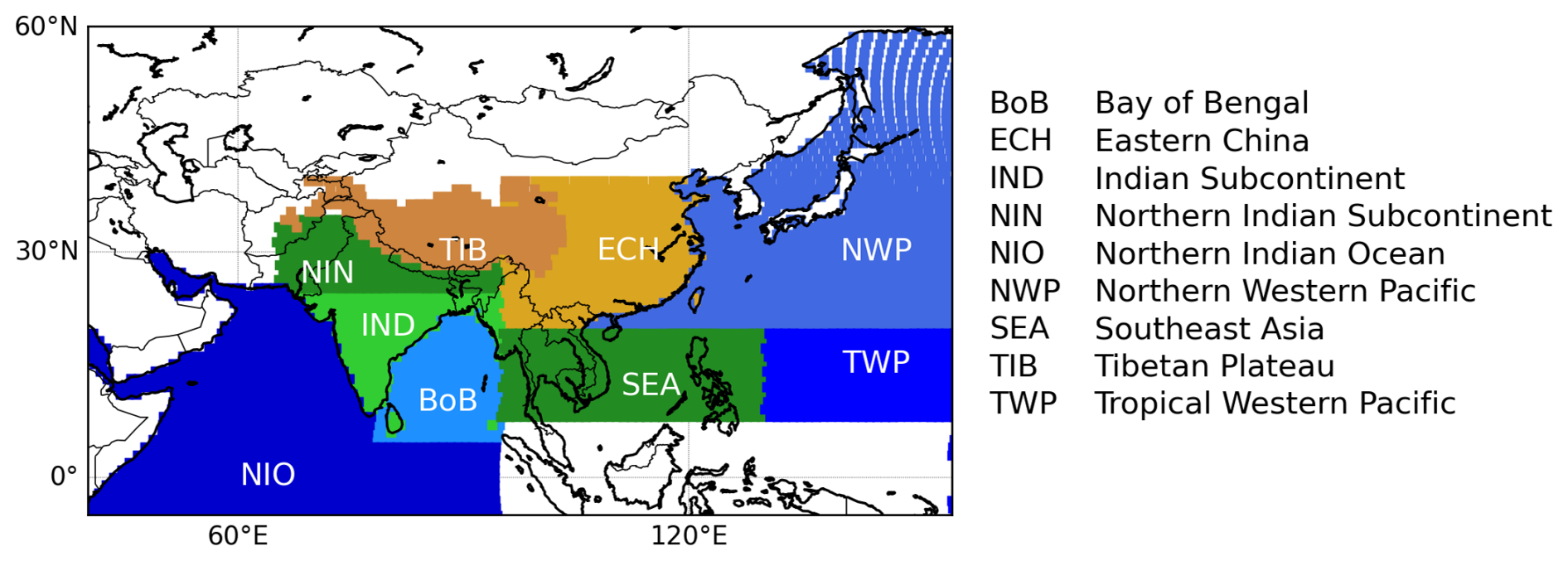
Figure 1 Map of surface-origin tracers used in the global 3-dimensional CLaMS simulation for 2023.

2.3 Measurement flights

A large filament of ASM air was predicted to approach the campaign base in Alaska on the 10 September 2023 UTC. The filament would remain close enough to the coast for two consecutive days to be in reach of HALO. Therefore flights on both 10 and 11 September 2023 were planned using the Mission Support System tool (MSS; Bauer et al., 2022) to measure the filament and the outflow of this first measurement. Figure 2 shows the CLaMS South Asia tracer at 360 K potential temperature as an indicator of air separated from the ASMA.

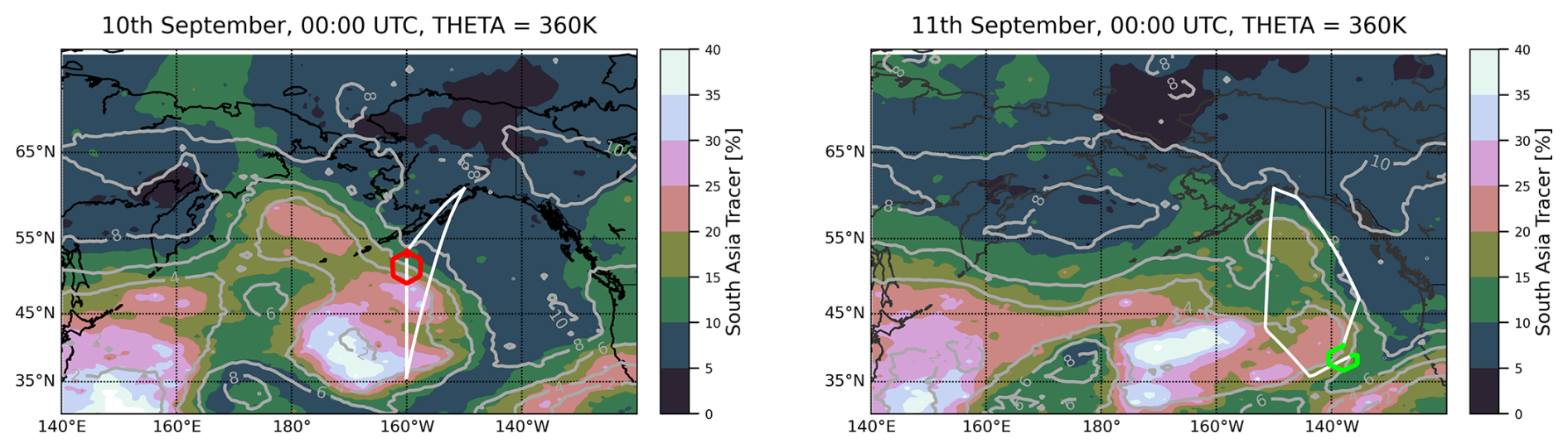
Figure 2 CLaMS South Asia tracer (= “ECH” + “TIB” + “NIN” + “IND” + “BoB” + “NIO”, see Fig. 1) at 360 K potential temperature. PV values are shown as gray isolines. (Left) Initial flight on 10 September 2023 UTC. A large filament with increased mixing ratios of South Asian air is projected to be in range of HALO research flights from the base in Anchorage. The first hexagon is located towards the end of the flight near the edge of the filament and is marked in red. (Right) Follow-up flight on 11 September 2023 UTC. The filament “rolls over” southeastwards. The second hexagon (marked in green) is located inside the outflow from the first hexagon (see Fig. 3) at that time.

Forecasts by the high resolution ICON model predict increased mixing ratios of several anthropogenic pollutants (not shown) such as PAN inside this filament, as well as a tropopause fold near the outer edge of the filament on 10 September 2023.

In order to perform a 3-D tomographic retrieval of the filamented air, a hexagonal flight path segment (referred to in the following as hexagon 1, indicated by the red path in Fig. 2, left panel) was included near the end of the first flight on the edge of the ASM filament. During the PHILEAS campaign, forward trajectory calculations using CLaMS driven by ECMWF forecasts were started for air parcels measured inside hexagon 1 to plan a second flight one day later with the aim of measuring the same air masses a second time (self-match). On the follow-up flight a second hexagonal flight path segment (referred to in the following as hexagon 2, indicated by the green path in Fig. 2, right panel) was flown around an area where many trajectories from hexagon 1 were matched. Inside hexagon 2 a cloud cover at around 10 km altitude partially limited the measurements of GLORIA towards lower altitudes, resulting in a section of the second hexagon volume not being observed. For the analysis of the GLORIA measurements, the CLaMS forward trajectories were recalculated using ERA5 (1° × 1°) reanalysis. Figure 3 shows these CLaMS trajectories connecting flights PH13 and PH14. In the following, air parcels which can be connected by trajectories between the two observed volumes are referred to as “matched”. Due to the high spatial resolution of GLORIA it is possible to study the changes and mixing that each matched air parcel undergoes between the two measurement flights.

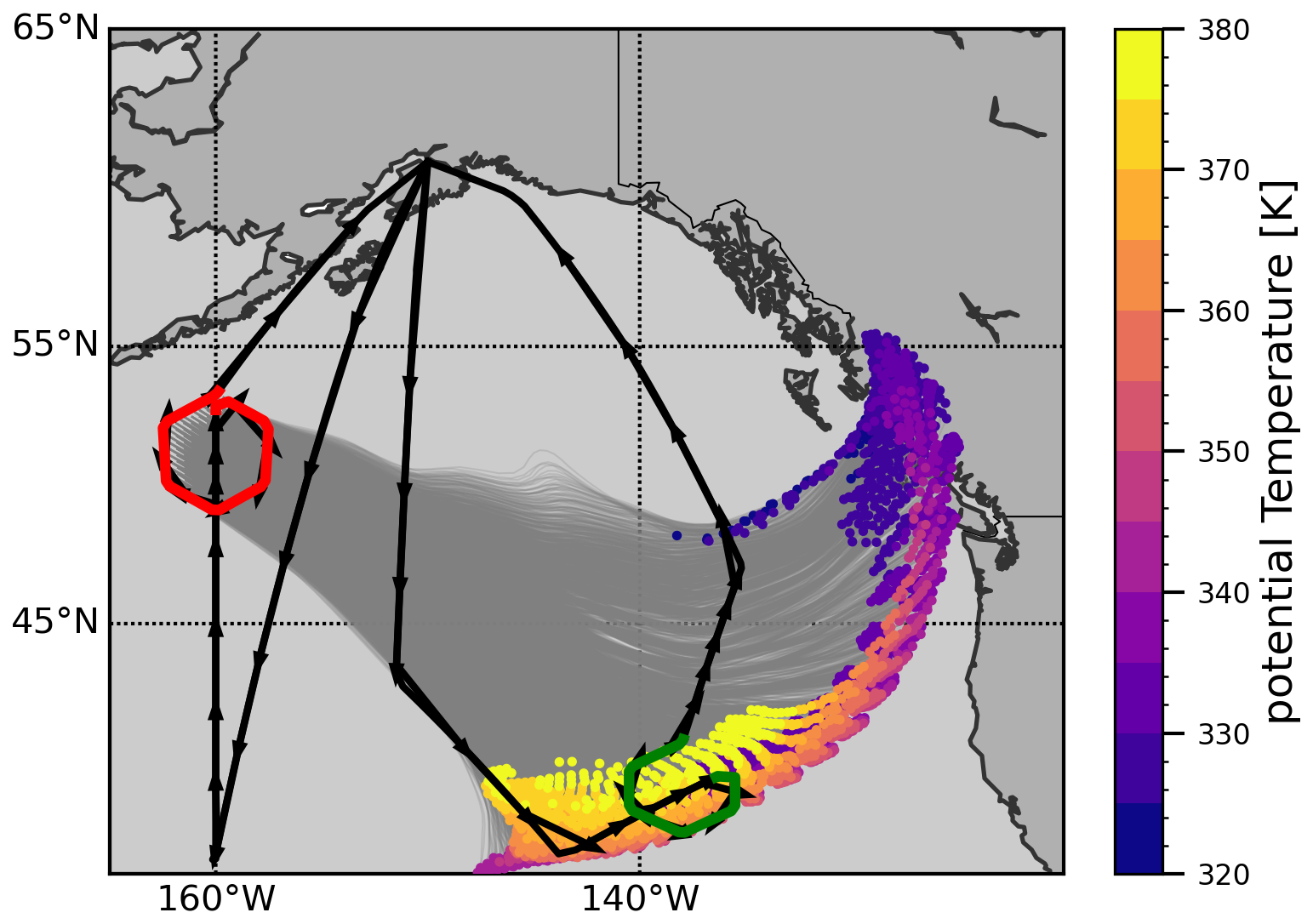
Figure 3 Self matching experiment during flights PH13 and PH14. The first hexagon is marked in red, the second hexagon is marked in green. Flight paths are shown in black lines, flight orientation is indicated by the arrows. CLaMS forward trajectories are shown as gray lines. They begin inside the first hexagon at 01:35 UTC and end at 01:50 UTC on the following day. The trajectories were started at every point on the retrieval grid and were driven by ERA5 (1° × 1°) reanalysis. Potential temperature of end points are shown in color-code. Trajectories were calculated for every point of the retrieval grid.

2.4 Analysis methods

In this analysis we present a novel classification approach for air masses based on statistical mixture models (see Sect. 2.4.2). This classification uses the chemical composition of the air masses only and is capable of identifying and quantifying an arbitrary amount of air types without the need of prior knowledge of their number or nature. Contrary to other clustering methods, mixture models inherently provide likelihoods for their classification. In this analysis these likelihoods directly convey information about the mixing of the observed air masses with different chemical composition. The data flow and the different steps of the classification are outlined in Fig. 4 and are discussed in the following text. More detailed overviews over the core concepts used in the classification are given in dedicated subsections below. The application of the concept to our measurements is described in Sect. 3.

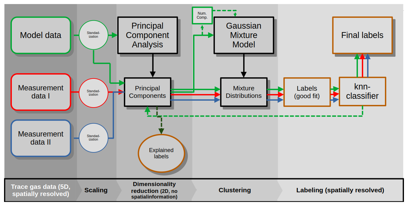
Figure 4 Schematic outline of the data pipeline. The workflow goes from left to right. Model data and their data products are indicated in green. Measurement data and their data products are indicated in blue and red, depending on which measurement. Transformations and classifiers, which are not explicitly dependent on a dataset, are marked in black. Transformations and classifiers, which explicitly depend on a specific dataset, are outlined in that dataset's color. Transformations and classifiers, which are applied to multiple datasets individually, are outlined in brown.

Different types of air can be distinguished by their unique chemical composition (trace gas mixing ratios), which is generally reflected in the correlation between the various chemical constituents (trace gases) (Plumb, 2007). Conversely, similar air masses show similar correlations. Thus, in a phase space which is spanned by each constituent (in this study: five different trace gases) similar air masses form clusters, with each cluster corresponding to one type of air present in the data. In a way, observed air masses can be interpreted as a collection of samples from different types of air. Their chemical composition is given by their location within the phase space. The number of types of air can be inferred from the number of these clusters. In this approach, neither the number of air types nor their chemical composition need to be known prior to the analysis, as their number can be determined by the number of clusters and their chemical composition from the location of each cluster. The only needed criteria are sufficiently many observations for clusters to form and sufficing dissimilarity between the air types for clusters to be distinguishable. Higher dimensional phase spaces tend to separate clusters better and thus as many non-collinear trace gases as possible should be considered. The correlations expected in a measurement could be inferred from model data, as model data tends to have less variation, which leads to more compact clusters. Such clusters can be determined with higher precision. Using model data also ensures a certain independence of the classification from the measurements itself. However, model data and measurements may not always be in good agreement. In such cases biases are introduced through the model data instead. An argument can be made for either choice. During preprocessing, each dataset (measurements or model data) is scaled to zero mean and unit variance individually following:

$$\begin{array}{}\text{(1)}& {\widehat{x}}_i=(x_i-{\mathit{\mu }}_i)/{\mathit{\sigma }}_i\end{array}$$

where μ_i is the mean and σ_i is the standard deviation of each dataset component. This ensures that each constituent has comparable numerical magnitude while preserving correlations. Therefore, different datasets can be compared regardless of their scales and potential offsets.

Next, the scaled model data is used to derive the subspace which retains the most information using the principal component analysis (PCA). The method is described in Sect. 2.4.1 in more detail. Using a lower dimensional subspace greatly increases the numerical stability of the later applied statistical mixture model and allows to focus on the most relevant components of the data. In particular, clusters in the full phase space generally remain clusters in the subspace. Here, a 3-D subspace is determined which retains the majority (92.5 %) of the data variance. The 3-D clusters (still representing different types of air) can be handled as being sampled from Gaussian distributions, which can be inferred (similar to fitting) by using a Gaussian mixture model (GMM), see Sect. 2.4.2. A GMM requires the number of clusters as an input parameter, which can be estimated directly from the 3-D subspace, see Sect. 2.4.3. The GMM directly provides the first two statistical moments of the probability density function for each cluster. In particular, the mean of each distribution as a point in the subspace describes the characteristic trace gas composition of the type of air associated with the cluster. The chemical composition (here, in 5-D) can be derived by applying the unique, inverse PCA transformation. The GMM provides the probabilities for each data point to have been generated by sampling from each cluster. Since each cluster usually lies suitably separated in phase space, these probabilities are mostly disjointed such that a unique label, being the most likely distribution, can be applied to each data point. Potential caveats to this labelling are discussed in Sect. 2.4.2.

2.4.1 Principal component analysis

The Principal Component Analysis (PCA) (Pearson, 1901; Hotelling, 1933; World et al., 1987; Jolliffe, 2002; Jolliffe and Cadima, 2016) is a method of dimensionality reduction of a dataset. It is commonly used to reduce high (N)-dimensional data to its core components and finds application in many natural sciences, such as biology and atmospheric science. Depending on the field it is also known under different terms, such as Karhunen–Loève transform in signal processing, and is strongly related to singular value decomposition in mathematics. The same method was already used to suppress noise in calibration measurements for the GLORIA instrument (Guggenmoser et al., 2015). The N-dimensional principal components c_i of a (N,k)-dimensional dataset (containing k observations of N features) X are the pairwise orthogonal vectors along which the internal variance of the data projected to that principal component is maximal such that $\mathrm{var}(\mathbf{X}\cdot {\mathit{c}}_i)>\mathrm{var}(\mathbf{X}\cdot {\mathit{c}}_{i+\mathrm{1}})$. Along the first principal component the data variance is thus maximal, with the second component having the second largest variance and so on. Components, along which the data variance is small, convey little information, and can thus be neglected. In particular, statistical noise conveys little to no information and is usually prevalent in the lowest principal components. Choosing an arbitrary cut-off n, the PCA provides an (N−n)-dimensional approximation of the data X still containing k observations which retains most of the original data's structure. The cut-off is usually chosen such that 80 %–90 % of the data variance is retained, following considerations described in Jolliffe and Cadima (2016). Since the PCA is a linear transformation, there exists a unique inverse transformation, albeit not without loss of a little bit of information due to the cut-off n.

2.4.2 (Bayesian) Gaussian Mixture Model

A statistical mixture model is a probabilistic model which describes a statistical population as the combination of many, statistically distinct sub-populations. In simple terms, given an N-dimensional dataset X, a mixture model assumes that the dataset X was generated by sampling from k random variables with N-dimensional probability densities $D_{\mathrm{0}},D_{\mathrm{1}},\mathrm{\dots },D_k$ with different (mixing) weights $w_{\mathrm{0}},\mathrm{\dots },w_k$ (Baxter, 2010). The statistical properties of each component distribution D_k are inferred directly from the dataset X. A Gaussian mixture model assumes each component distribution to be a Gaussian distribution 𝒩. The mixture distribution from which X was generated is then given by:

$$\begin{array}{}\text{(2)}& \begin{array}{rl}& D\left(\mathbf{X}\right|{\mathit{\mu }}_{\mathrm{1}},\mathrm{\dots },{\mathit{\mu }}_k,{\mathbf{\Sigma }}_{\mathrm{1}},\mathrm{\dots },{\mathbf{\Sigma }}_k,w_{\mathrm{1}},\mathrm{\dots },w_k)\\ & =\sum _{i=\mathrm{0}}^k{w}_i\cdot (\mathrm{2}\mathit{\pi }{)}^{-\frac{N}{\mathrm{2}}}\cdot {\det }_i({\mathbf{\Sigma }}_i{)}^{-\frac{\mathrm{1}}{\mathrm{2}}}\\ & \cdot \exp \left(-{\displaystyle \frac{\mathrm{1}}{\mathrm{2}}}(\mathbf{X}-{\mathit{\mu }}_i{)}^T{\mathbf{\Sigma }}_i^{-\mathrm{1}}(\mathbf{X}-{\mathit{\mu }}_i)\right)\\ & =\sum _{i=\mathrm{0}}^k{w}_i\mathcal{N}\left(\mathbf{X}\right|{\mathit{\mu }}_i,{\mathbf{\Sigma }}_i)\end{array}\end{array}$$

where ${\mathit{\mu }}_i,{\mathbf{\Sigma }}_i,w_i$ are the mean vector, covariance matrix and mixing weight of each component, with $\sum _{i=\mathrm{0}}^k{w}_i=\mathrm{1}$. The number of components k is the free parameter of the statistical mixture model. In Sect. 2.4.3 a method to estimate this parameter from the data itself is presented. In contrast to a regular Gaussian mixture model, which determines its parameters using expectation maximization (Dempster et al., 1977), a Bayesian Gaussian mixture model (BGMM) determines its parameters via variational inference. The necessary a priori values for this Bayesian approach can be provided by a Dirichlet process. A trained BGMM provides probabilities for each data point x according to Eq. (2). Since it is assumed that a point necessarily must have been sampled from any of the distributions, these probabilities can be normalized:

$$\begin{array}{}\text{(3)}& p_i\left(\mathit{x}\right)={\displaystyle \frac{w_i\mathcal{N}\left(\mathit{x}\right|{\mathit{\mu }}_i,{\mathbf{\Sigma }}_i)}{\sum _{j=\mathrm{0}}^k{w}_j\mathcal{N}\left(\mathit{x}\right|{\mathit{\mu }}_j,{\mathbf{\Sigma }}_j)}}\end{array}$$

A BGMM can also be used as a classifier by assigning each point x a label according to the most likely component the point was sampled from. The label is assigned according to:

$$\begin{array}{}\text{(4)}& l\left(\mathit{x}\right)=\mathrm{argmax}\left(\log \right(w_k)+\log (\mathcal{N}\left(x\right|{\mathit{\mu }}_k,{\mathbf{\Sigma }}_k\left)\right)\end{array}$$

The maximum value of Eq. (3) then corresponds to the probability that the point was accurately labeled. For disjoint distributions Eq. (3) typically takes values between 1 (high confidence) and 0.5 (ambiguous labeling between two classes). In the following we refer to this quantity as the class alignment.

The classifier works well for all points which have suitably high probabilities to be sampled from any one of the component distributions and thus are well represented by the model. If points are not well represented by the model, each probability 𝒩_i vanishes and Eq. (4) is dominated by its second term. Labels are then determined by which distribution 𝒩_i vanishes the slowest, regardless of the mixture weights w_i, which leads to sudden changes in labeling on the edge of phase space. Since each Gaussian distribution is compact in phase space the labels should be compact similarly. To account for this behaviour we determine labels using Eq. (4) only for points with at least one sufficiently high probability and determine labels for all other points using a nearest-neighbor classifier. Only few points require such a correction and the resulting labels are compact in phase space.

2.4.3 Feature-number estimation

The majority of clustering algorithms have free parameters p which are chosen by the data analyst, thus introducing human judgement. A Gaussian mixture model requires the number of components as such a free parameter. A way to a more objective selection and to deriving an estimate of these parameters from the data itself is to iterate a classifier over various possible choices and compare the resulting classification scores. The estimate itself should not explicitly depend on the particular classification score. A suitable choice for many classifiers is the silhouette score (Rousseeuw, 1987), which describes how dissimilar a data point within one class is to the points outside of that class compared to the data points within the class. The silhouette score becomes maximal if the points within each class are most similar to each other while being most dissimilar to points outside of that class, e.g. if the classification reflects the data structure well. Increasing the number of classes does not necessarily increase the silhouette score, as splitting a class of similar points is penalized due to reducing dissimilarity to points in other classes. The parameters p for which the silhouette is maximal indicate the highest agreement between the data and the underlying model of the classifier.

3 Results and Discussion

3.1 GLORIA measurements of Asian Summer monsoon outflow

An overview of the observations from hexagon 1 is shown in Fig. 5. The first row shows the retrieved mixing ratios of PAN for three diametrical cross-sections through the retrieval volume. The second row shows the same cross-sections but for the values of the CAMS model, which has a 1° by 1° horizontal resolution and 250 m vertical resolution in the relevant region.

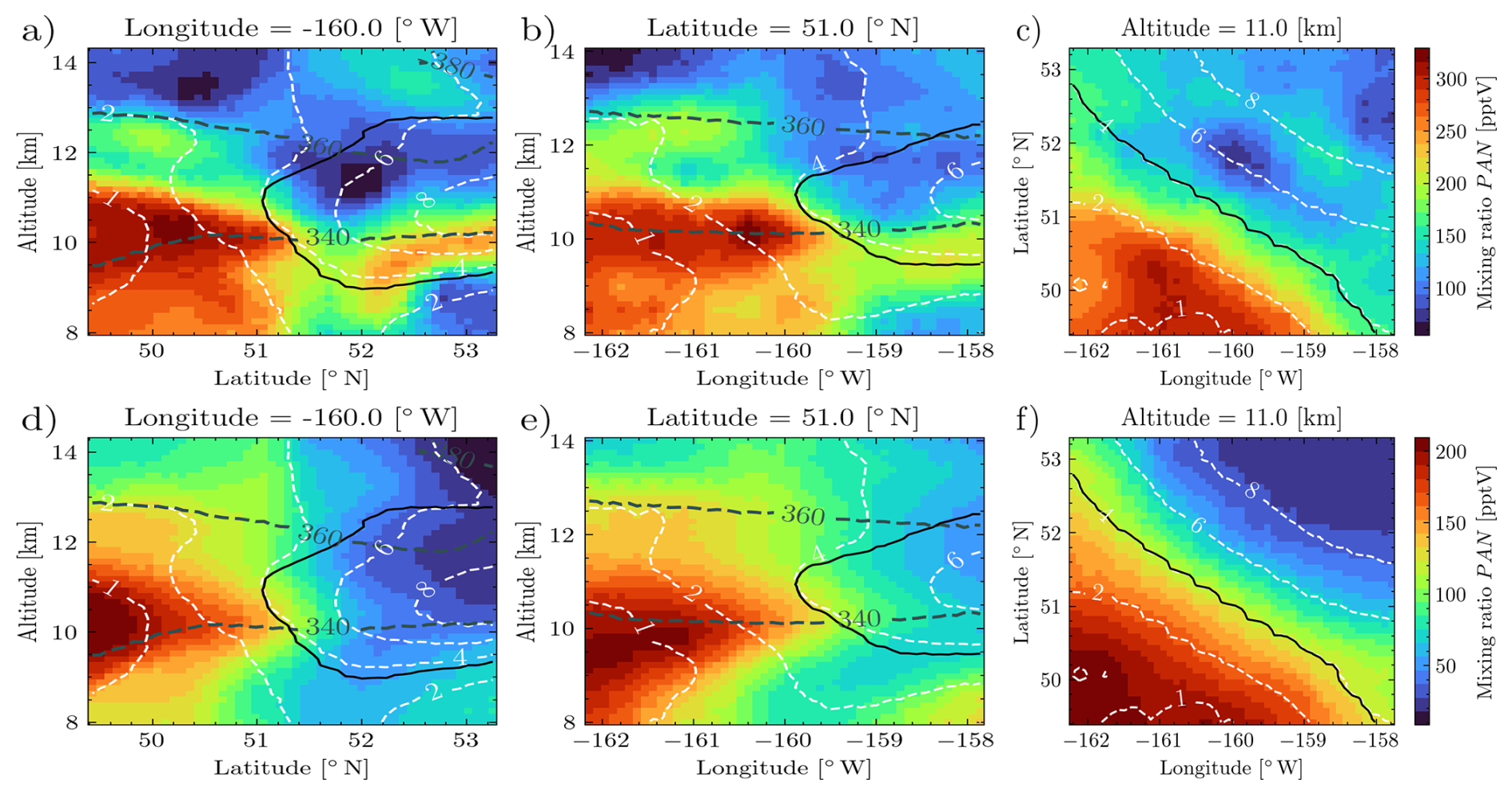
Figure 5 PAN mixing ratios inside the first hexagon on 10 September 2023 (upper row: GLORIA retrievals; lower row: CAMS model predictions). Shown are two vertical cross-sections (left and middle) and one horizontal one (right). PV isolines are shown as white dashed lines, potential temperature isolines are shown as gray dashed lines. The dynamical tropopause adapted from Kunz et al. (2015), which determines the PV-value depending on the potential temperature based on climatological data, is indicated as black line in all panels.

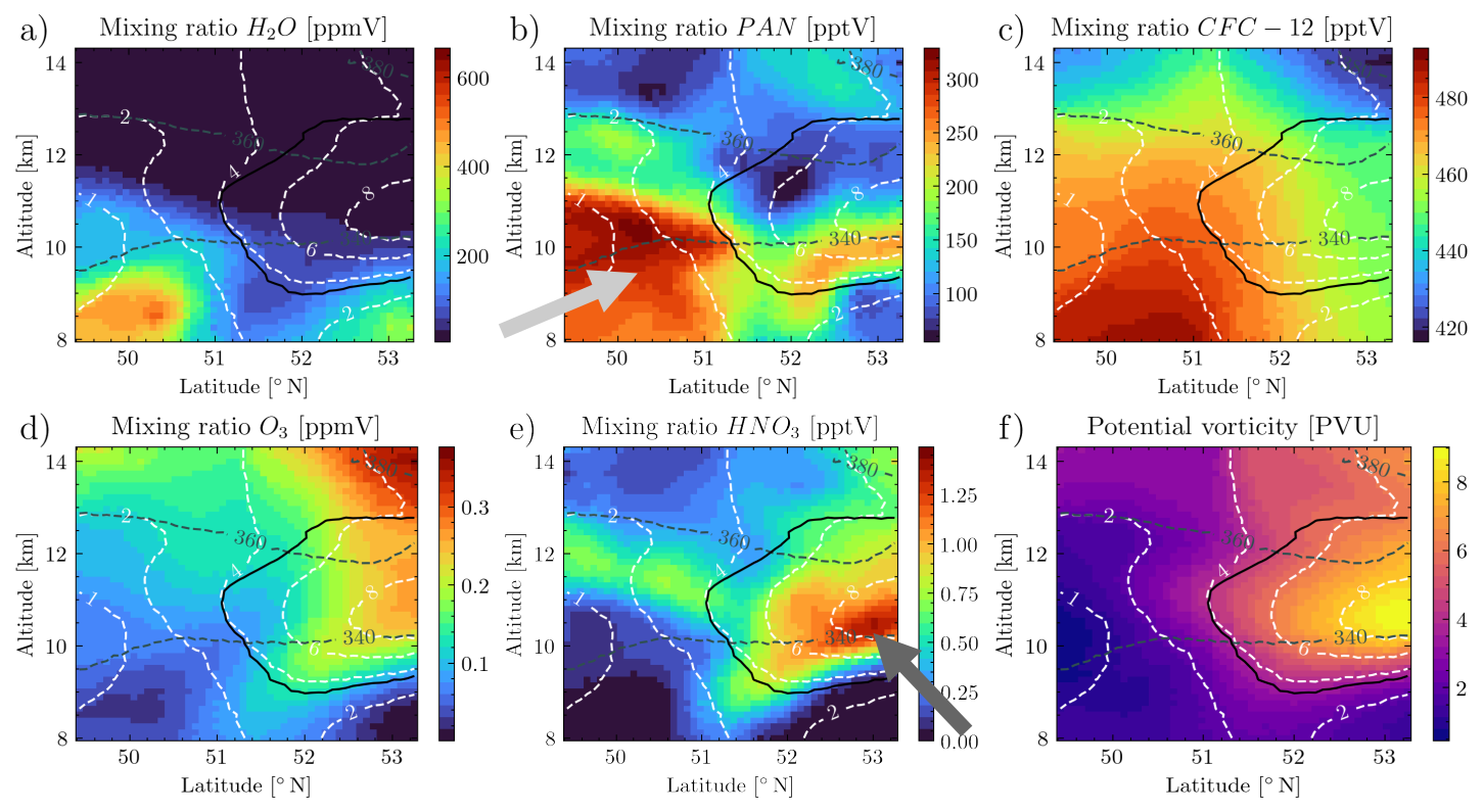
Figure 6 (a–e) Retrieved trace gas species inside the first hexagon (10 September 2023 UTC). (f) Potential vorticity derived from ERA5 reanalysis. The cross-section shown is the same as in Fig. 5a. The backgrounds are interpolated along constant longitude of 160° W. The dynamical tropopause and PV-isolines are indicated as black and white lines, respectively.

For all panels the dynamical tropopause is calculated for September according to the climatological values in Kunz et al. (2015) on the relevant isentropes, based on PV values from ECMWF ERA5 reanalysis data, and is shown as a black line. Additionally, PV isolines are shown as white lines, potential temperature isolines are shown as gray lines.

As already mentioned in Sect. 2.3, increased mixing ratios of PAN are indicators for the outflow of the Asian Summer monsoon. The filament is located on the low latitude/western side of the hexagon at altitudes between 13 km down to at least 8 km (panel b, light arrow) in accordance with the flight planning predictions. It contrasts against the surrounding air through steep gradients. The general shape and size of the filament is in good agreement with the model predictions, although the predicted mixing ratios are up to 50 % lower than the observations. Smaller scale features are not adequately resolved by the model, and therefore small scale mixing is unlikely to be correctly resolved as well. In particular, the measurements show much stronger gradients than e.g. the CAMS simulation. This indicates that model values may not be suitable to use for the following classification.

The low values of PAN on the high latitude/north-eastern side of the hexagon suggest stratospheric air, which extends downward to around 11 km. This stratospheric air is located not as low as the CAMS model had predicted. The PV values mostly reflect this structure, with a 3-PVU isoline would encapsulate most of the distinct features well. There is a distinct feature of increased PAN on the north-eastern side of the hexagon at around 10 km, which lies inside the stratospheric air mass/intrusion according to the dynamical PV-tropopause (panel e, dark arrow). The other observed trace gases show similar patterns, but with several apparently conflicting features, as shown in Fig. 6 exemplarily in the same cross-section as Fig. 5a–e. The filament is visible in the retrieved H₂O, but only extends upward to around 11 km, which is around 1 km lower than PAN would suggest, which can be explained by the freezing out of water near the tropopause. O₃ and HNO₃ reflect the filament as well, with low values localized around the same region, but the low O₃ values would suggest an extent to much higher altitudes. HNO₃ shows a layer of increased mixing ratios in the upper part of the filament, but reveals low values again above that layer, indicating a more tropospheric character of these air masses. The feature of increased PAN to the north-east is completely missing in H₂O, while both stratospheric tracers show increased values in this region as well. This already indicates mixing of different air masses, e.g. of aged tropospheric air and fresh stratospheric air, as will be elaborated on in the next section. CFC-12 on the other hand shows very little structure at all (cf. the narrow range of the color scale), except for lower values around this feature.

The observations therefore indicate that there is an active mixing between the UT and LS occurring inside the intrusion. However, the dynamical situation is not adequately characterized by neither the dynamical tropopause (shown in Fig. 6), nor the thermal tropopause (not shown here) or any singular or pair of tropospheric and stratospheric tracers. A physically complex situation such as this requires a more rigorous classification which exploits as much available information as possible. Our approach bases on the methods introduced in Sect. 2.4 and is applied in the following section (Sect. 3.2).

3.2 Classification

3.2.1 Classification and Identification

The classification analysis described in Sect. 3.2 is applied to the retrieved trace gas mixing ratios of H₂O, PAN, O₃, HNO₃ and CFC-12. Due to the aforementioned issues of models to resolve the finer structures/mixing we use only the retrieved values in the first step of the classification. Spatial information such as longitude, latitude or potential temperature was not considered in the classification. The standardization parameters used for each dataset and the resulting principal components are given in Tables A2 and A3, respectively. We estimate that there are five distinct features in the retrieval data using the method described in Sect. 2.4.3. The BGMM is thus trained assuming five mixture components. Labels are determined using the method described in Sect. 2.4.2.

The resulting classification for both hexagon retrievals are shown in Fig. 7.

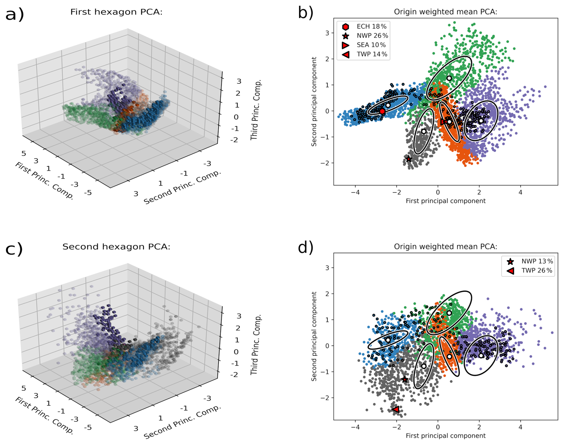
Figure 7 BGMM classification based on the first three principal components. (a, c) PCA of hexagon 1 and hexagon 2, respectively. (b, d) Visualization of the first two principal components of hexagon 1 and hexagon 2, respectively. For each Gaussian distribution a 1σ environment is indicated by ellipses. The PCA of the weighted mean of each measured trace gas weighted by the relevant surface-origin tracers of the CLaMS simulations are shown in red markers. The red markers for “SEA” and “TWP” in (b) lie close to each other and basically overlap. The percentages shown are the maximum percentage of each respective surface-origin tracer. In all panels the classes found by the BGMM are shown in color-code. Air parcels, which were observed in both hexagons are indicated by a black outline. For each class the cluster center is indicated by white dots.

The choice of 5 classes is well reflected in the transformed retrieval data with five distinct clusters of points visible in Fig. 7a. Shown are the cluster centers of each class, which correspond to the average chemical composition of each class. Each class lies well separated from each other and the labelling is unambiguous for the majority of points, with approximately 1 % of points requiring label adjustment. The classification of hexagon 2 is shown in Fig. 7c). For better visualization, the first two principal components of each hexagon PCA are shown in Fig. 7b and d. It should be noted that clusters may overlap in this visualization due to perspective. Given that hexagon 2 was measured in a dynamically similar, but temporally later situation, the PCA deviates from hexagon 1 in several ways. The blue and gray clusters are much less distinct from each other. An argument can be made to consider them merged into a new cluster, which we will only do visually for consistency reasons. The green and orange clusters also converge in hexagon 2, implying that mixing resulting in similar air masses is occurring. The effect is most visible for those points having positive values for the principal components. Unfortunately, no air parcels lying in this region were revisited and consequently these changes were not observed directly. It shall be noted that while the orange cluster in hexagon 1 shares a large border with the violet cluster and might be considered an extension of the later, the local correlations in both clusters are quite different, meaning key chemical components may be similar, but show distinct differences in their proportions.

For each class the cluster centers (shown as white dots in Fig. 7b, d) represent the mean values of points in each class. These cluster centers are basically the mean values of each class and can be considered representative for the whole class, which will be further explored in the following. Similar to these representative points for each class, representative points for the contribution of each Asian monsoon source region can be constructed by taking the weighted mean of the observation weighted by the surface-origin tracers (see Sect. 2.2). These values are then transformed and shown within the PCA in Fig. 7b and d as red markers. The positions where these transformed points are located within the PCA show which source region at the Earth's surface has the largest impact to the respective classes.

To express this classification in physically relevant terms, the inverse transformation of the PCA is applied to each cluster's center as the most representative point to transform the point back into regular tracer composition. The resulting characteristic chemical composition of each class is shown in Fig. 8 in percentiles of the total distribution.

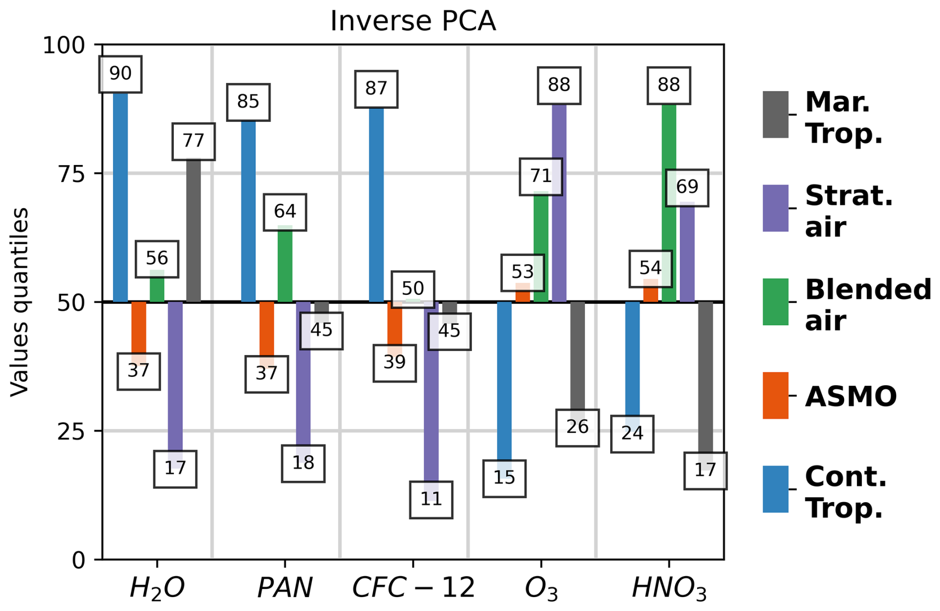
Figure 8 Chemical composition of each cluster center by the inverse PCA transformation. Shown are the mixing ratios of each trace gas expressed in percentiles of the overall distribution. Each value is shown at the end of each bar. A value of 20 for H₂O indicates that 20 % of all measured values of H₂O are lower than this value. Each bar is shifted by 50 such that lower than average bars are pointing downwards and above average bars point upwards.

When considering both the information of these characteristic compositions of each class and the information about the regions of origin aligned with each class, a physical interpretation of each class can be made:

• Continental tropospheric class: this typically tropospheric air (blue label) shows the by far highest mixing ratios for each tropospheric tracer and the by far lowest values for each stratospheric tracer. High water vapor and high PAN/CFC-12 indicate a deep tropospheric character, possibly from within the ASM region, which the surface-origin tracers link to continental regions such as the Eastern China region. We refer to this type of air as continental tropospheric air (CT).

• Maritime tropospheric class: this typically tropospheric air (gray label) is most similar to the tropospheric class (1) with respect to all tracers except PAN and CFC-12, which are significantly lower, indicating less pollution contained within, likely from less industrious regions or less populated ones. Indeed, in contrast to the CT class it appears to be linked to more maritime sources such as the North-Western Pacific region and is thus referred to as the maritime tropospheric air (MT).

• Stratospheric class: the typically stratospheric air (violet label) shows the by far lowest values for each tropospheric tracer and the by far highest values for each stratospheric tracer. The vanishing moisture is the strongest indicator. The fact that no surface-origin tracer corresponds to this air type further supports this characterization. We refer to this type of air as stratospheric air (S).

• Asian Summer monsoon outflow class: the air associated with the orange label shows moderately low values in both tropospheric and stratospheric tracers. Its composition is clear distinct from either tropospheric or stratospheric air and therefore cannot be either. To preempt the succeeding analysis this class is localized precisely in those section of the hexagon where the filament was predicted during flight planning. The regions most aligned with this air type are the East China (ECH) region and the Tropical West Pacific (TWP) region, further suggesting a link to the ASM outflow. Additionally, comparing the surface-origin tracers to the localization of this class (see Fig. B4) it shows that this class contains the highest mixing ratios of relevant surface-origin tracers. The strong signatures of both ECH and TWP indicate a mixing of these air masses even before the formation of the filament. The CLaMS simulations do indeed show this mixing of TWP air with the outer regions of the ASMA (see Vogel et al., 2026). The chemical composition is consistent with such an interpretation. We refer to this type of air as ASMO air (A).

• Blended class: the air associated with the green label shows a unique composition with moderately increased tropospheric tracers except for CFC-12, which is average, and increased stratospheric tracers. Its composition can be understood as a mixture of tropospheric and stratospheric air. It is located in hexagon 1 in the lower part of the observed stratospheric intrusion and appears folded underneath the stratospheric air in hexagon 2 (see Fig. 9). Since the extra-tropical tropopause generally acts as a transport barrier, this degree of mixing is likely induced by the intrusion. As the air types of this classification may not be arbitrarily unique, it stands to reason to assume that any other mixture of tropospheric/stratospheric air would appear similar, e.g. air from the outer anticyclone, where exchange between tropospheric and stratospheric air can occur. To avoid unnecessary confusion we will refer to this air type as “blended”' air (B) instead of mixed air.

3.2.2 Localization

The classification was derived from the chemical composition only and did not have direct information of the three-dimensional spatial distribution of the different trace gases/classes within the hexagon. If the classification and its interpretation are meaningful, the spatial distribution of the classes is expected to be consistent with this interpretation.

The spatial structure of each class is illustrated in Figs. 9 and 10.

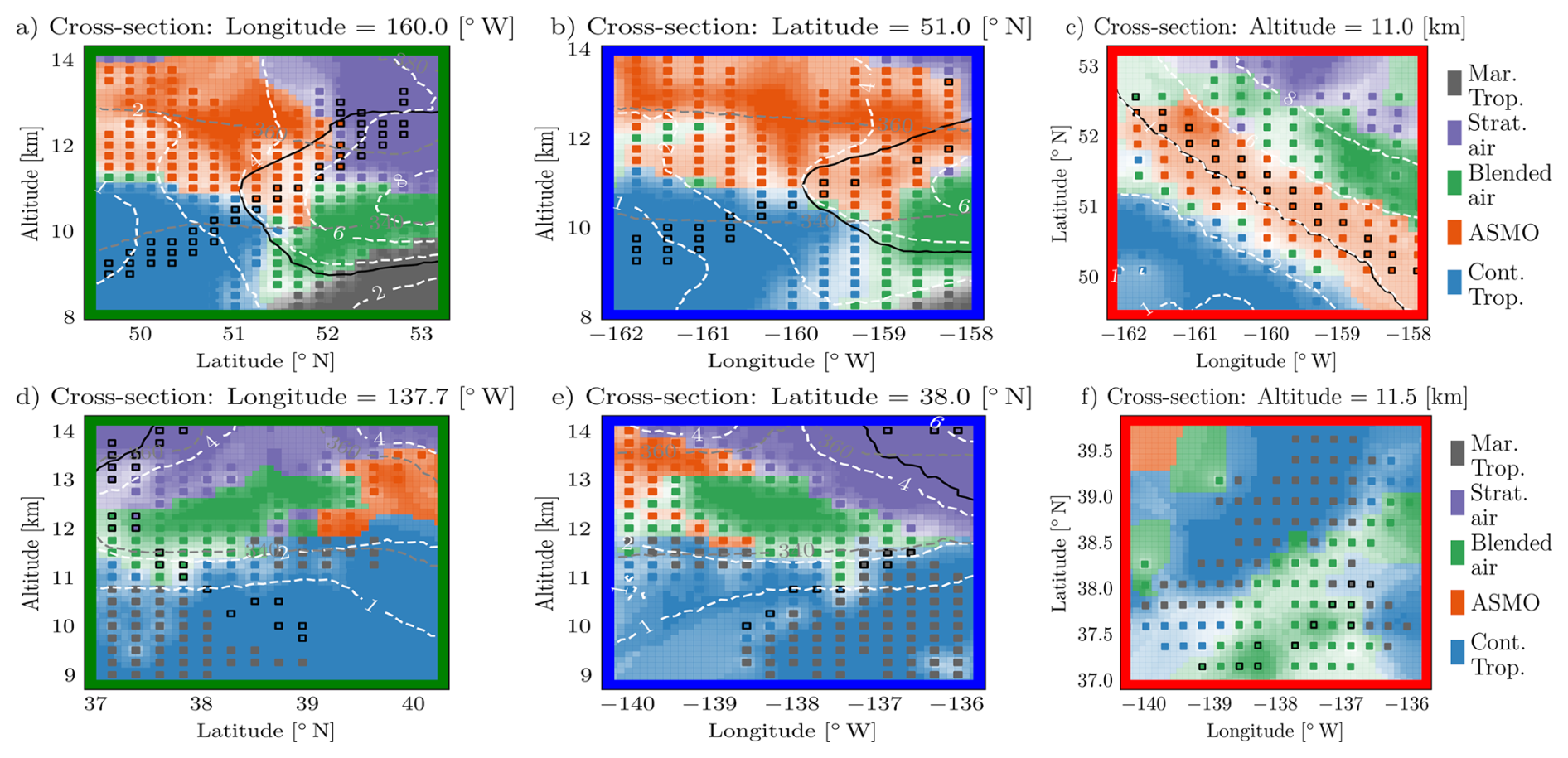
Figure 9 Class distribution inside (a, b, c) hexagon 1 and inside (d, e, f) hexagon 2. Cross-sections are identical to Fig. 5 and are indicated in Fig. 10. The dynamical tropopause is indicated as black line. PV isolines are shown in white. Measurement points within each cross-section are shown as solid markers. Matched points are indicated by black borders. Class assignment is indicated in color-code, with high class alignment shown in more opaque colors. In hexagon 2 the background of both tropospheric classes are displayed in blue as if they were a single class. For clarity gray labeled points are still shown in gray. The background shows the classification applied to the trace gases interpolated in each cross-section. Spaces containing few measurement points are more uncertain.

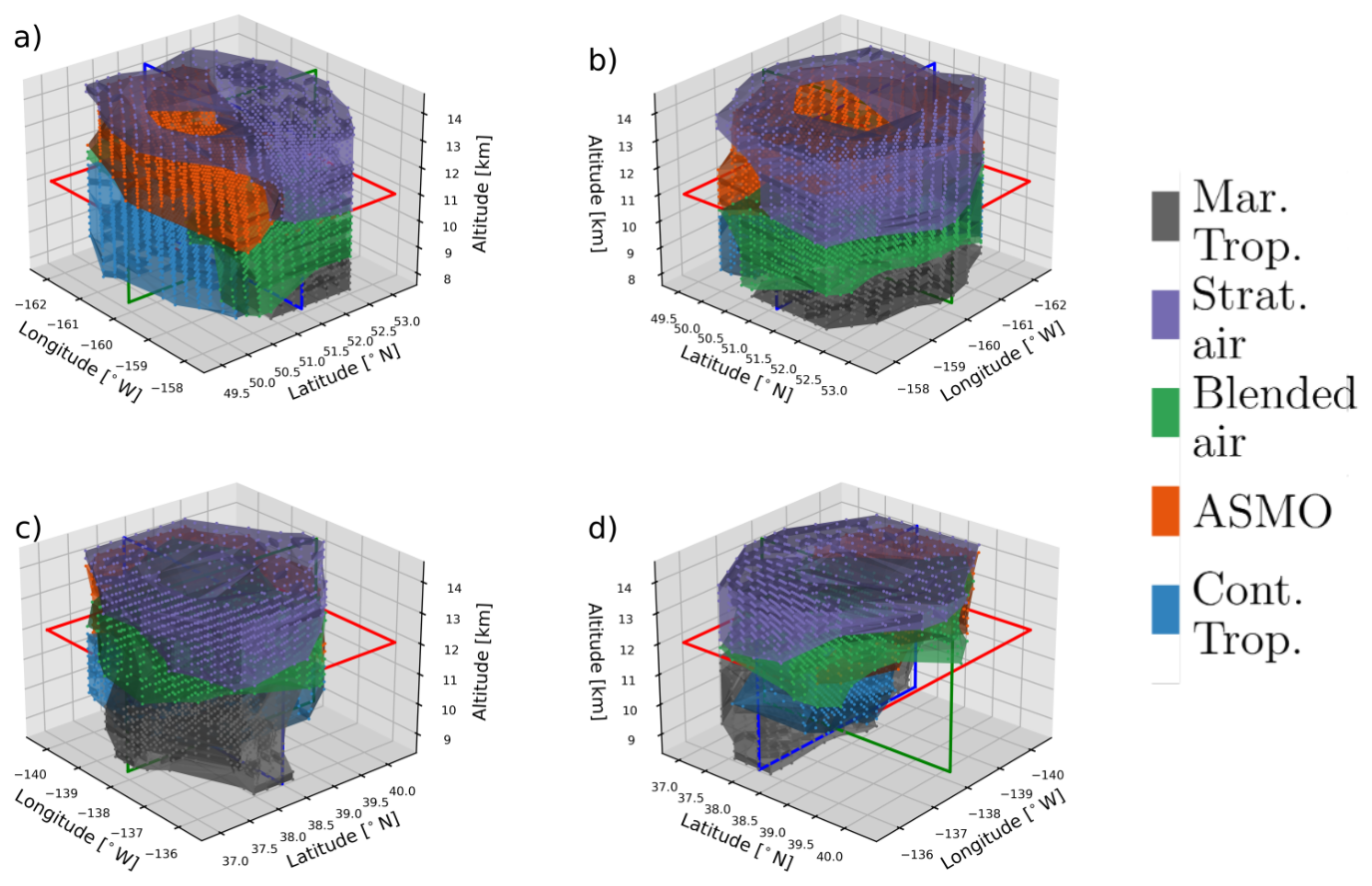
Figure 10 3-D visualization of class distributions (a, b) within hexagon 1 and (c, d) within hexagon 2. The second image is rotated by 90° relative to the first image in each row. Shown are the concave hulls of each class (α=1), tangent points are indicated as points. The cross-sections shown in Fig. 9 are indicated by the colored rectangles.

Panels (a) to (c) in Fig. 9 show the class distributions of hexagon 1 along the same cross-sections used in Fig. 5. Their position within the hexagon is shown in Fig. 10a and b. The background in between measurements in these cross-sections is interpolated on the retrieved values and positions. These interpolated values are then transformed and classified as described before. A high probability for the class assignment is shown in bright colors, lower probabilities (corresponding to labeling ambiguity) are shown in pastels or white. Regions which contain few measurements are most influenced by interpolation, but generally reflect the class structure well due to the compactness of the PCA. Air parcels revisited between the two flights are indicated by black outlines. Figure 10 illustrates the full spatial structure of each class. In particular, each class does form a compact region not only in phase space, but also in real space (in the atmosphere), despite no spatial information was used.

The tropospheric classes CT and MT are at the lowest altitudes and are mostly located below the 2-PV isoline, which is commonly used as an upper limit for the troposphere. In hexagon 2 this behaviour is most consistent. In hexagon 2 both tropospheric classes lie intertwined, suggesting mixing of maritime and continental tropospheric air occurs. This mixing (merging) of those air types was already suggested by the classification in Fig. 7d. In the following both tropospheric classes are considered functionally the same (and referred to simply as the tropopheric class (T)) and are indicated in blue color. Conversely, the stratospheric class is located in the highest altitudes. Due to the tropopause fold in hexagon 1 the vertical structure is distorted, which is correctly captured in the classification, in which the CT class and the S class lie diametrically opposed. Comparing the location of the ASMO class to Fig. 2, the ASMO class coincides with the location of the filament in both hexagons, further justifying the identification of the class with ASMO air. In hexagon 1 an intrusion of ASMO air into the stratosphere is seen (panel b). This suggests inmixing of ASMO air directly into the lower stratosphere. The blended class is located bordering the ASM air filament between the troposphere and the stratosphere, mostly at the tip of the stratospheric intrusion. Visually it appears as if the blended class acts as a partially dissolved extension of the intrusion. This characterization would be in line with its chemical composition. As stated beforehand, this classification is not necessarily unique, and the blended class could also be the mixing of ASMO air with stratospheric air. Neither point can be substantiated further from this analysis alone.

Active mixing between classes is directly indicated by reduced probabilities of class assignment, as the transition from one class into another crosses the regions of low class assignment probability. Considering these probabilities as shown in bright and dark colors in Fig. 9, mixing is occurring near the edges of most classes in either hexagon. Edges with still high probabilities imply only recent contact between those air masses, such that mixing has not yet sufficiently occurred. The strongest ongoing mixing is occurring in hexagon 1 between the CT class and the A class/B class. In hexagon 2, however, the strongest ongoing mixing however is between the blended class and its bordering classes. For those air parcels which were observed in both hexagons the mixing processes can be derived explicitly by comparing their chemical composition in both hexagons.

3.3 Mixing processes

The matching experiment was designed to observe the same air parcels on two successive days (self-match flight). In total 396 such matched air parcels were observed based on their trajectories, corresponding to around 10 % of all observed air parcels.

Changes in the chemical composition of these matched air parcels give insight into the mixing processes, as little to no changes in chemical composition are expected over the course of 24 h for any of the observed trace gases. Changes in composition are therefore most likely due to mixing. The characteristic chemical composition derived above of each type of air involved can be used to validate. The BGMM classification directly implies different types of mixing processes via the changes in class assignments between hexagon 1 and 2. We consider mixing both due to changes in class assignment (Sect. 3.3.1) and due to changes in trace gas mixing ratios (Sect. 3.3.3).

3.3.1 Qualitative mixing analysis

Mixing in the form of changes in classification are summarized in the confusion matrix in Fig. 11.

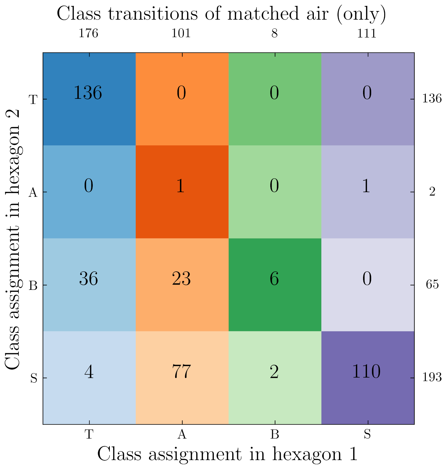
Figure 11 Confusion matrix of class assignment of matched air parcels. The number of each transition is shown in each matrix element. The columns indicate the class assignment of all air parcels in hexagon 1, the rows indicate the class assignment of all air parcels in hexagon 2. The air types are indicated by the abbreviations (T, A, B, S) introduced in Sect. 3.2. Both tropospheric classes (CT and MT) are combined into one (T). Each possible transition has a unique color variation of the color used to encode its class assignment in hexagon 1. The total number of parcels in each class in hexagon 1 and 2 are indicated on each row/columns edges, respectively.

A confusion matrix summarizes each possible combination of two instances of labeling, here the labels in hexagon 1 and 2. The column i indicates the label in hexagon 1 (X), the row j indicates the label in hexagon 2 (Y). The number of transitions of that kind are then given by the matrix element i,j, which in the following is referred to as “X-Y”. Each class is abbreviated by their first letter as defined above. A transition X-Y would indicate air of type X is becoming of type Y. Air type Y is not necessarily the air type X is mixing with, but simply the resulting air type. If the mixing is relative slow air type Y is likely the air type X is mixing with. In general not every possible combination is observed. Therefore, most elements are zero. Elements with very few transitions can indicate issues with the trajectories or with the classification and are not considered significant. It is however not to say that these transitions are not real. From the confusion matrix qualitative insights into the mixing processes can be derived:

A large share of blended air is created via the transitions T-M and A-B. The transition B-B is observed, but rarely. ASMO air also transitions into stratospheric air via A-S in large quantities. There are no significant transitions X-A, where X is any other class, which lead to the creation of ASMO air, which again supports the characterization as ASMO air, as Asian Summer monsoon should be the product of the monsoon and not a product of mixing. The transition “T-S” sticks out as a direct transition of tropospheric air into stratospheric air without observed intermediate state, which is likely related to a classification issue, as no tropospheric air lies directly bordering the stratospheric air. The lack of this transition would also reflect the transport barrier between the troposphere and the stratosphere in the extra-tropics Otherwise most tropospheric air and stratospheric air do not undergo significant changes due to mixing (T-T and S-S).

The transitions T-B and A-B stand out because when considering the average chemical composition of the classes T, A and B (see Fig. 8), neither T air nor the A air contain sufficiently much stratospheric tracers such that B air could have been created due to mixing from any combination of T, A and B air. The deficit of stratospheric tracers requires at least some S air to make up this deficit. A possible explanation would be the transition A-S, which has consistent increases in both O₃ and HNO₃. The chemical budget would add up if A air would partially mix with S air, and afterwards mixes with T air creating B air. How these transitions would happen in detail, e.g. which intermediate states occur, cannot be derived from these observations. Otherwise, an additional source of O₃ and HNO₃ would be required, which is investigated in Sect. 3.3.3.

If more than two mixing partners are involved in such a process, these intermediate states would no longer be mixing lines, as is traditionally considered, but rather mixing curves of more complex shapes. This would explain why the phase space in Fig. 7a somewhat resembles a traditional mixing curve (in 3-D), but few to no explicit mixing “lines” are contained.

3.3.2 Localization of mixing processes

Due to the 3-D tomographic retrievals the spatial structure of the changes in chemical composition, which implies the mixing, is known as well. The spatial structure of each transition is shown in Fig. 12.

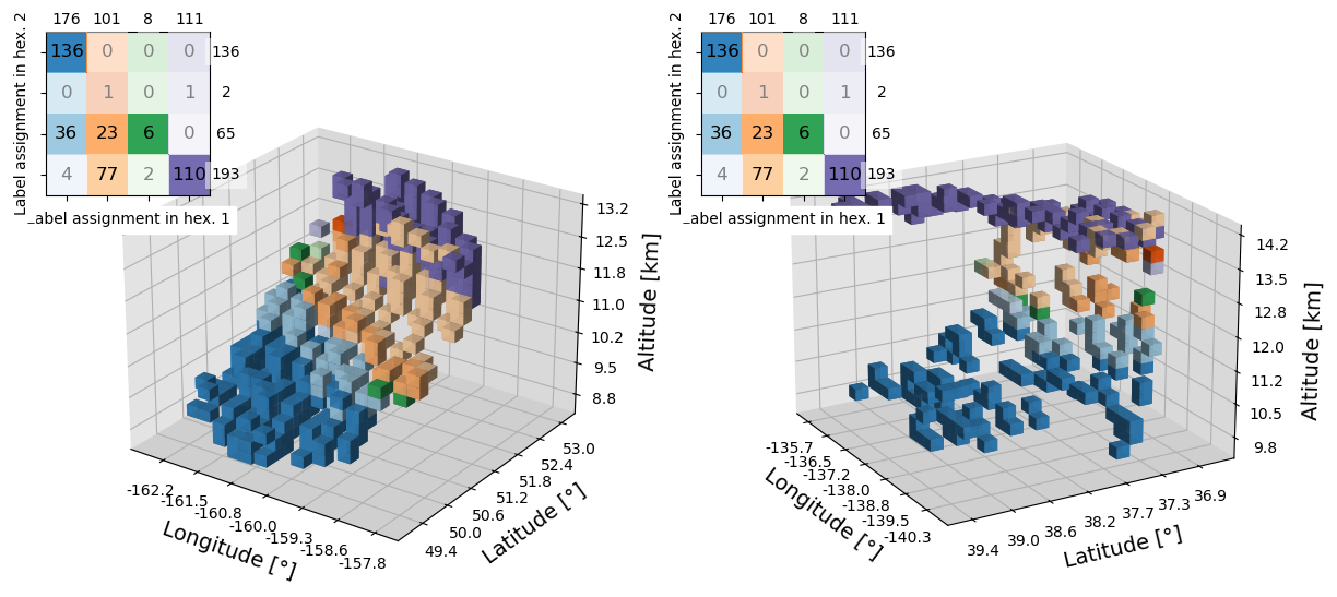
Figure 12 Visualization of transition states. (Left) Trajectory starting points inside hexagon 1. Transition state is indicated in color-code, see legend. (Right) Trajectory end points inside hexagon 2. Transition state is indicated in color-code consistent with Fig. 11. Rare and missing transitions are grayed out for visibility.

The mixing processes are structured as follows: the transition T-T is located in the lowermost altitudes purely within the troposphere in both hexagons, which extends up to 9.5 and 11.2 km, respectively. This represents the transport of air within the troposphere. Above the troposphere lies a layer of blended air from around 9.5/10.5 to 11/11.2 km. The blended layer itself consists of two individual layers, which meet at around 9.7 km in hexagon 1. The lower layer is created from the transition T-B, the upper layer is created from the transition A-B. In hexagon 2 the lower blended layer is stacked similarly, but the upper blended layer is much more interwoven with the stratospheric air originating from A-S.

Above the blended layer lies a layer of ASMO air A, which transitions into stratospheric air and extends to the stratosphere at around 12/13.5 km. Upwards lies the stratosphere with transport within itself. Each transition again forms coherent regions, with the transition B-B being a small exception. Despite the spatial distortion observed in hexagon 1, each transition follows a stratified vertical structure. The exchange between the troposphere and the stratosphere appears to be still mostly vertical, despite the perturbation caused by the tropopause fold most likely inducing the mixing being mostly horizontal. The stratification of the mixing can be explained by the dynamical properties of the atmosphere, which counteracts the distortion. The mixing of tropospheric air and stratospheric air via ASMO air occurs over a larger vertical range, which could imply that said distortion is indeed necessary to initiate this tracer exchange.

3.3.3 Quantitative mixing analysis

So far the mixing processes have been explained by considering changes in complex correlations via PCA. Since for each matched point there are measurements in both hexagon 1 and 2, the direct changes for each observed tracer can be considered as well.

Quantitative insights into the mixing processes can be derived from the autocorrelations in Fig. 13a–g.

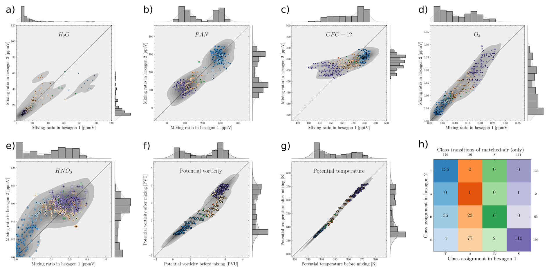
Figure 13 (a–e) Overview of tracer changes between the two hexagons. The identity (no changes) is shown in the background as line. The different transitions are indicated in color-code in accordance to the confusion matrix shown again in (h). Uncertainties due to retrieval parameters are shown as well (small). Histograms of measurements are shown on the edges. A Gaussian kernel density estimation is shown as shade. (a) The value range for H₂O is artificially limited to focus on low values. (f) Changes in potential vorticity (ERA5 reanalysis data) during mixing. (g) Changes in potential temperature (ERA5 reanalysis data) during mixing.

The potential temperature (panel g) shows the isentropic nature of the mixing. Since the measurements were derived from a retrieval we estimate their uncertainties by applying a rigorous Monte-Carlo approach to determine the influence of different factors on the retrieval result. A detailed overview over the exact methodology can be found in Ungermann (2013) and Ungermann et al. (2022). The uncertainties are generally small compared to the variance in the measurements. Investigating the retrieval diagnostic reveals that the results are dominated by observations, with little influence of the a priori (not shown). Since H₂O can condense out, it is generally not a well conserved quantity and therefore not very descriptive for the mixing processes. Such effects appear to be visible for the tropospheric water vapor, which sees significant reductions in between flights. The changes in PAN divide the matched points into two groups, the tropospheric air and everything else. It stands out that the stratospheric air, (in hexagon 2) which was created from the ASMO air (in hexagon 1) contains significantly more PAN than the other stratospheric air, further substantiating the transport of tropospheric tracers into the lower stratosphere via filaments of ASMO air. O₃ shows no such structures and basically reflects the vertical structure. The potential vorticity decreases for the transition A-S and remains fairly constant otherwise. HNO₃ shows significant increases within the troposphere, with the largest increases in the transition T-B, which is to be expected considering the change in class. Such increases are utterly unexpected and considering the other stratospheric tracer O₃ cannot be explained by directly mixing with stratospheric air. While HNO₃ shows the largest uncertainties of all retrieved species, such uncertainties cannot explain this increase.

A potential source for HNO₃ within the atmosphere are lightning storms, which may have occurred in between flights. Tie et al. (2001) state that lightning events can lead to increases of up to 300 pptV in HNO₃ compared to the background, which lies in the order of magnitude of observed increases. Observations by the GOES-18 satellites allow to link possible lightning activity in the region to the observed increases in HNO₃. Figure B1 in Appendix B shows the cumulative lightning events between the 10 and 11 September 2023. Each white dot indicates a lightning signal picked up by the satellites. The hexagons and the trajectories of the outflow are indicated similarly to Fig. 3. Those trajectories, which see these significant increases in HNO₃, are marked in orange. There are multiple lightning events that come close to or intersect with the trajectories. Such lighting activity may very well be the reason for the increases in HNO₃. Given that such changes in HNO₃ are not due to mixing, a reevaluation of these transitions assuming constant HNO₃ seems reasonable. We find that most transitions remain the same, the strongest effect is in the transitions T-B, which shows 30 air parcels in this transition that would remain tropospheric air, and the transition A-B, in which 18 air parcels would remain ASMO air. The transition A-S appears largely unaffected by this. However, we cannot isolate the effect of lightning activity from changes due to mixing and therefore cannot draw any additional conclusions with certainty.

4 Summary and conclusions

The Asian summer monsoon is one of the most important circulation systems of the northern summer hemisphere. It represents an effective pathway of tropospheric air originating from the southern Asian continent into the upper troposphere and lower stratosphere. This pathway is to date only partially understood and quantified. Through Rossby wave breaking events large filaments of Asian monsoon outflow are transported westward into the mid-latitudes, where they are eventually mixed into the lower stratosphere. By distributing pollutants globally, such mixing has an effect on the global climate.

During the PHILEAS campaign in late summer 2023 a filament of Asian summer monsoon outflow was measured on two consecutive days with the GLORIA instrument. The edge of the filament was tomographically imaged in 3-D during the first flight. Based on CLaMS trajectory calculations, air masses from this filament edge were revisited inside a second 3-D tomographic observation on the next day (Fig. 3). The chemical composition of the filamented air has been retrieved in the trace gases H₂O, PAN, O₃, HNO₃ and CFC-12 in 3-D spatial resolution unique to the GLORIA instrument. The instrument's high spatial resolution allows to follow single air parcels and thus to study the change of the chemical composition of these parcels over time. We showed the complex spatial and chemical structure of an ASM filament close to a stratospheric intrusion. The dynamical tropopause is distorted such that it did no longer reasonably reflect the observed chemical structure.

We present a novel classification method, which is based on statistical mixture models. Using this classification we are able to discern the number and the characteristic chemical properties of distinct types of air based only on trace gas observations. The classification reflects the spatial structure of the observed atmosphere without prior knowledge of it. The classification works with arbitrary number of air types and provides highly non-linear boundaries, but generally requires multiple simultaneous trace gas observations. Due to the statistical nature of this classification regions of ongoing mixing can be discerned already by the classification confidence.

We find a distinct type of air strongly linked to the Asian summer monsoon both by its location within each hexagon and by surface-origin tracers from Lagrangian transport simulations with CLaMS used to identify the Asian Summer monsoon outflow. By investigating the changes in classification of each revisited air parcel, we identify mixing pathways of the filament. Our observations show mixing of air appearing to be ASMO air directly into the lower stratosphere where the two air masses connect physically. Of 101 air parcels classified as ASMO air, 76 % of them show this transition. We observe that anthropogenic pollutants such as PAN are transported into the lower stratosphere this way. A blended state with strong tropospheric and stratospheric influences is also observed as a relatively stable state.

We are able to measure some air parcels in both hexagons and for those air parcels changes in chemical composition are presented in 3-D both for the classification and for each tracer individually. From our observed mixing processes the blended state is only possible by mixing both tropospheric and stratospheric air. While no direct mixing of stratospheric air into this mixed air is observed, and because the spatial structure of the mixing does not imply it, the mixing likely involves the ASMO air, leading to a 3-way mixing of tropospheric, stratospheric and ASMO air. Such complex mixing structures are supported by the analysis of the chemical phase space of the observed air masses. The ASMO air can be linked to the South East China region and the Tropical Western Pacific region. While it shows a certain similarity to the stratospheric air measured, its unique chemical composition is distinct from it. Both maritime and continental tropospheric air can be linked to the North West Pacific region and the East China region, respectively. Thus, the influence of these individual areas on the Asian summer monsoon outflow is illustrated.

We observe significant increases in HNO₃ for many tropospheric air parcels which cannot be explained through mixing alone due to the relatively small changes in other tracers during mixing. By using lightning events observed by the GOES-18 satellites, we are able to link such increases to lightning activity between both flights. The hypothetical effect of such lightning is most pronounced in classifying air as blended instead of their previous class, but has little to no effect on other transitions.

Combining many different trace gas species allows to draw a much more complete picture of the atmosphere, which conventional methods simply cannot. This self-matching experiment was conducted to demonstrate the measurement capabilities of the Earth Explorer 11 candidate CAIRT (ESA, 2023, 2025), which at the time of writing of this study was not selected for the mission. The wide range of trace gas species observable by CAIRT and its capability to perform 3-D resolved measurements would have been ideally suited to study mixing processes. A conceptionally similar instrument STRIVE is in development and will be deployed no earlier than 2030 (NASA, 2026). It will be capable of performing similar experiments and will be able to provide additional insights into the mixing processes in the UTLS region and the ASM.

Appendix A: Technical details

A1 Effect of elevation angle on retrieval results

Due to the distance of several hundred kilometers between the GLORIA instrument and the observed air masses, small changes in the elevation angle can lead to several hundred meters difference when trying to locate an air parcel and its trajectory. Therefore, the effect of the elevation angle on the matching must be considered. From the multiple calibration methods available a small range of plausible elevation angles between 0.02 and 0.05° was selected. In Fig. A1 the auto-correlation for both retrieved as well as model values for any combination of plausible angles are summarized. We operate under the assumption that over a span of 24 h little changes are to be expected. Larger changes should be supported by larger changes in the model values as well.

Comparing each configuration we find an elevation angle of 0.04° for hexagon 1 and an elevation angle of 0.03° (second row, third column) to be most consistent among model predictions and retrieval results. The effect of other, but similar combinations of angles, however, is not pronounced.

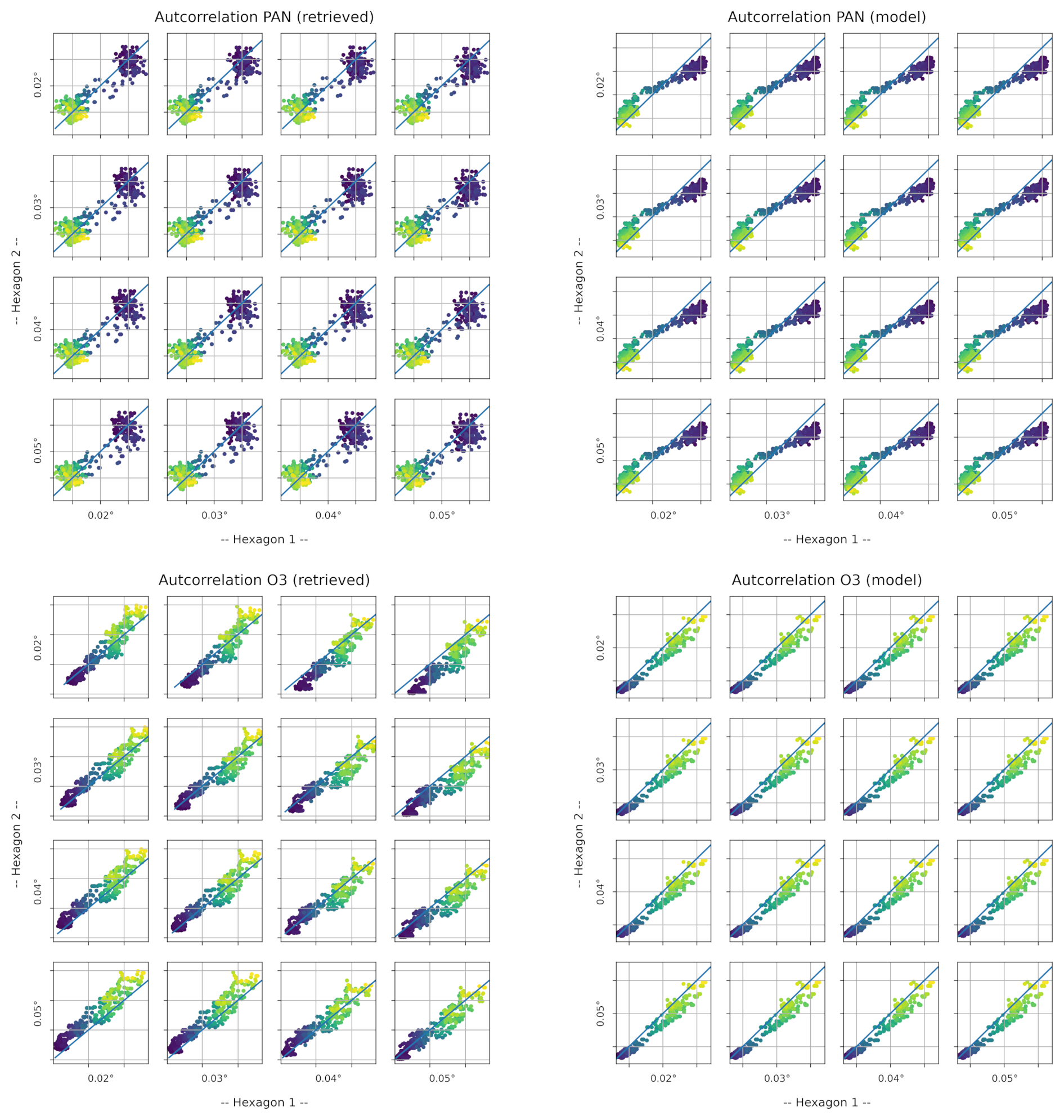
Figure A1 Comparison of different elevation angles on trajectory matching. (Left) Retrieval results in hexagon 1 vs. hexagon 2 given a combination of elevation angles for PH13 and PH14. (Right) Same, but for model values. Shown are PAN and O₃ representatively.

A2 Spectral windows used for tomographic retrievals

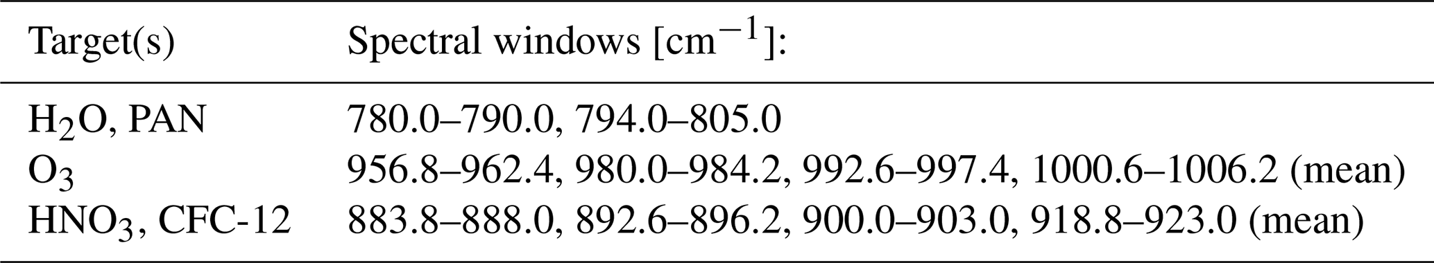
The spectral windows used to retrieve the trace gas species are listed in Table A1.

Table A1 Spectral windows used for retrieval of different trace gases.

A3 Data scales and principal components

The data scales and the principal components used in the analysis are shown in Tables A2 and A3, respectively.

Table A2 Standardization parameters for each dataset. μ denotes the mean values, σ denotes the standard deviation of each respective trace gas species.

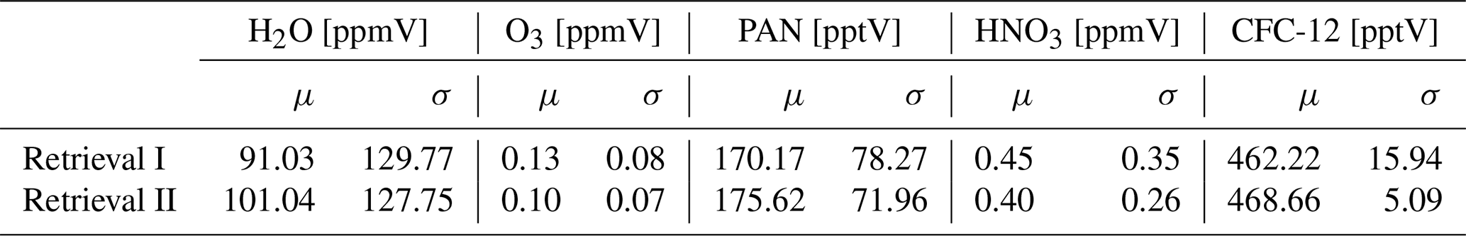
Table A3 Principal components used in the classification. Each contribution refers to the scaled data, which was scaled using the parameters found in Table A2. For the classification described in Sect. 3.2 only the first three components were used.

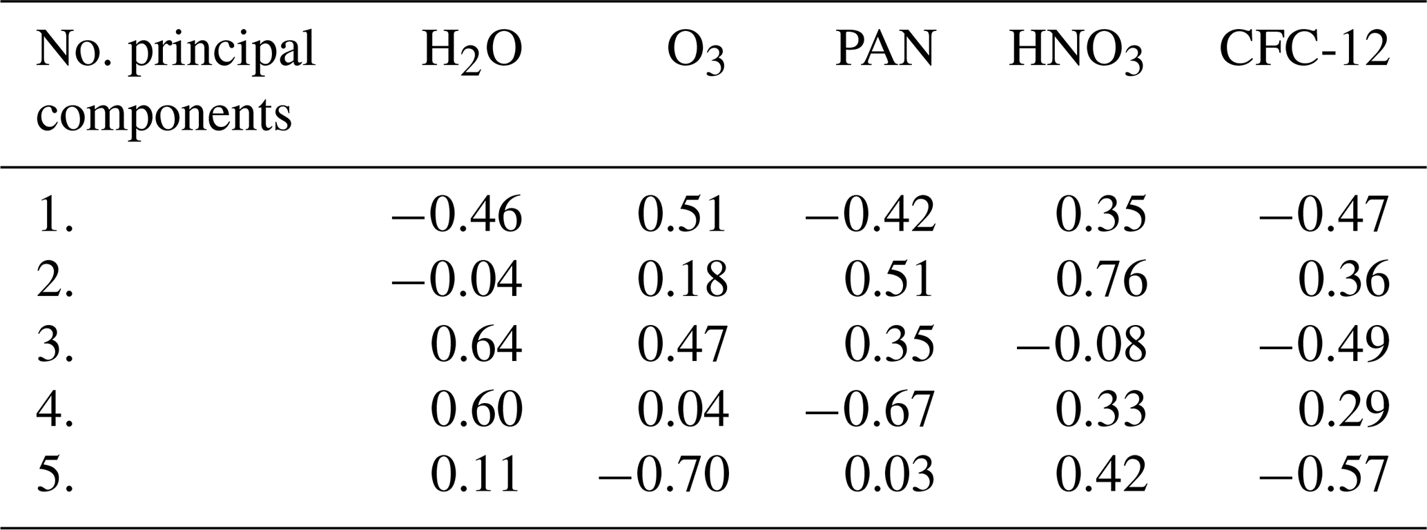
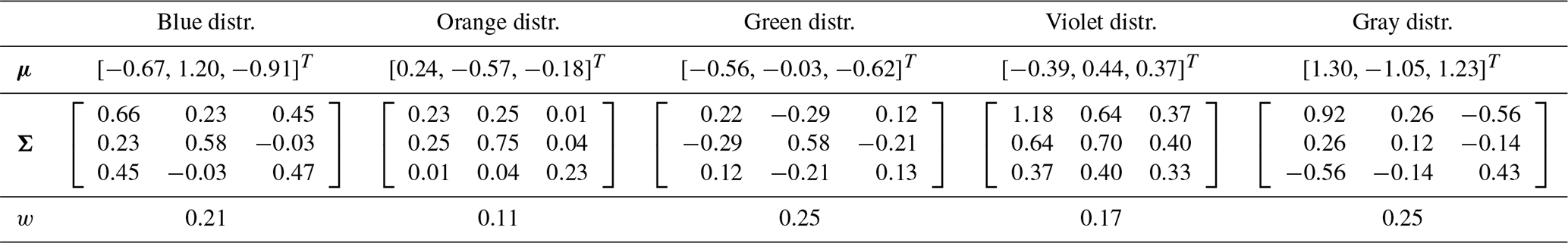
Table A4 Statistical parameters of each component distribution used in classification. Each quantity is expressed in standardized coordinates. μ denotes the mean values of each component, Σ denotes the covariance matrix of each component and w denotes the mixture weight of each component.

Appendix B: Complementary material

B1 GOES-18 lightning events between both flights

In Fig. B1 all lightning events observed by the GOES-18 satellite network in the time between both measurement flights are illustrated. The intensity of these events are neglected. The time-resolution of the observations are also not considered, as created HNO₃ can be mixed into the air masses followed by our trajectory calculations, especially on smaller scales.

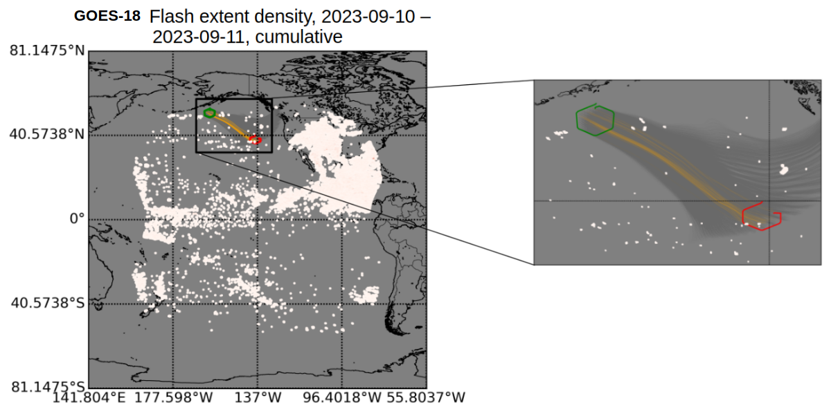
Figure B1 GOES-18 lightning events. Shown are all events that have occurred between PH13 (hexagon 1, green) and PH14 (hexagon 2, red). The trajectories are indicated in gray lines. A zoomed in section of the geographically most relevant region is shown to the right. Trajectories, which show significant increases in nitric acid are marked in orange.

B2 Tropopauses and PV in hexagon 1

In this analysis it was stated that both the dynamical tropopause and the thermal tropopause do not reflect the tracer distribution in hexagon 1 well, mostly due to the spatial distortion of the tropopause fold. The point is illustrated in Fig. B2. The dynamical tropopause, which is derived from both potential temperature and PV values, shows the tropopause fold mostly due to the anomalous distribution of PV, see Fig. 6f. The form of this PV abnormality is illustrated in Fig. B3. The observed PV abnormality is not limited to the hexagon volume, but extends beyond that. This already indicates that a climatological definition of the dynamical tropopause may not reflect the observed situation well. The thermal tropopause, following the standard definition by the World Meterological Organization (WMO), extends above the retrieval volume, leading to only the small portion (northwards of 51° N and eastwards of −159° W) to be classified as stratospheric. In particular, many regions with increased stratospheric tracers lie below this tropopause. A secondary tropopause is observed, similar to Vogel et al. (2016). Since both definitions are mostly contradictory to each other and fail to reflect most of the observed chemical structure, it was decided to not rely on any of these definitions in this analysis.

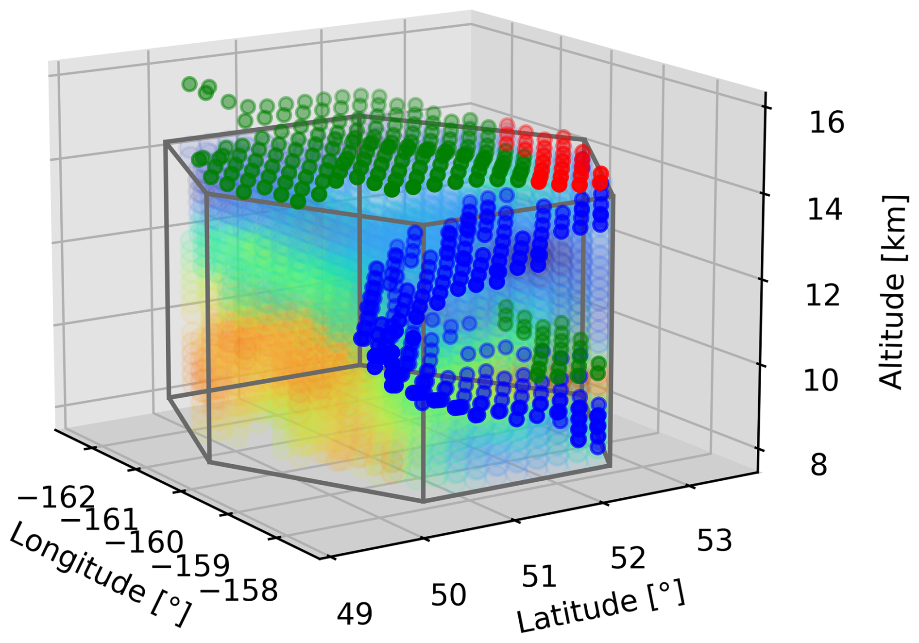
Figure B2 Visualization of the conventional tropopauses in hexagon 1. The (first) thermal tropopause at the footprint of the hexagon is shown in green. The secondary thermal tropopause is shown similarly in red. The dynamical tropopause, adapted from the climatological information in Kunz et al. (2015), is shown in blue. The mixing ratios of PAN are shown in color-code.

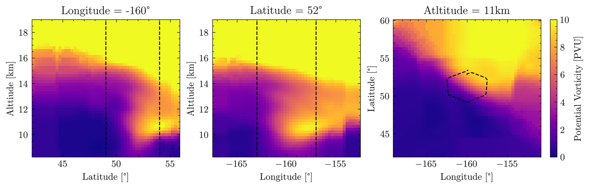
Figure B3 Overview of the PV distribution near hexagon 1. Shown are the same cross-sections used in Fig. 5a–c, but extended both horizontally and vertically. The horizontal borders of hexagon 1 are indicated as black lines. The PV values were again taken from ERA5 reanalysis data. The color-scale is consistent with Fig. 6f.

B3 Correlation between surface-origin tracers and classification

The surface-origin tracers indicating the influence of certain surface regions on the observed air masses are shown in Fig. B4 for a select cross-section. Comparing these cross-sections to Fig. 9a, it illustrates the statement made in Sect. 3.2.2 that certain labels are indeed deeply correlated to certain surface-origin tracers. Due to the discrete nature of the labels this correlation is otherwise difficult to illustrate. A particular point made in this analysis is the identification with the orange (ASMA) class with air containing a large share of Asian Summer monsoon outflow. The classification as such was justified through its chemical composition, which does not match any other air type anticipated in this particular region of the atmosphere, the lack of creation of this air type via the observed mixing processes, and the coincidence of this air type with the filament of ASM outflow. Figure B5 shows the distribution of the SEA surface-origin tracer for the remaining cross-sections in comparison to the distribution of the classification. The coincidence between the SEA surface-origin tracer and the ASMO class is consistent and reliable across all cross-sections. A point is made in the analysis that this ASMO class may have significant stratospheric influence due to mixing before the observation. While this cannot be refuted in this analysis, we can clearly differentiate between the ASMO class and the stratospheric class, for which the surface-origin tracers are vastly diminished.

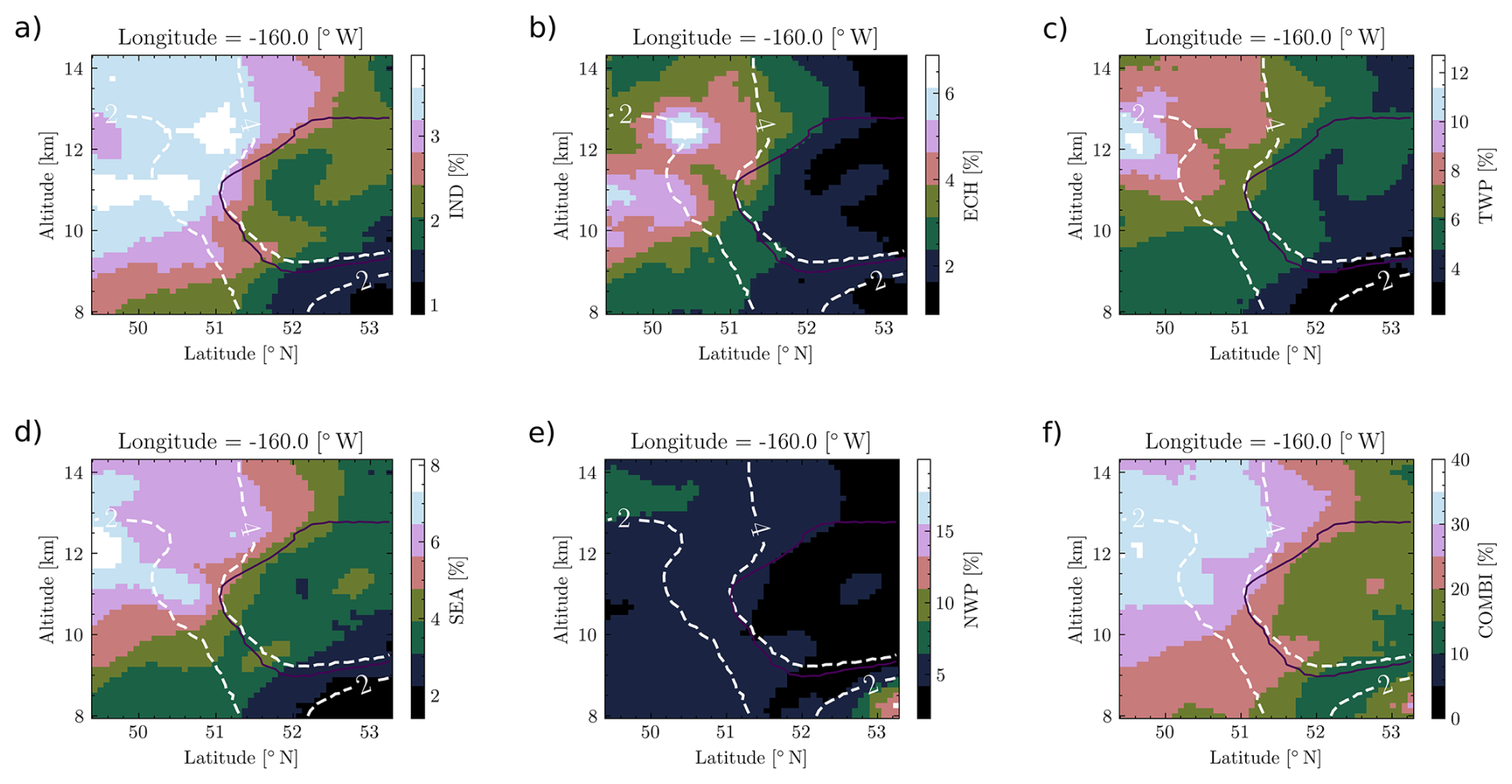
Figure B4 Cross-sections of selected surface-origin tracers. The cross-section corresponds to Fig. 5a. The tracers shown in (a)–(e) are the most significant (most retained) tracers also shown in Fig. 7b and d as representative points. The South Asia tracer used during flight planning (shown in Fig. 2) is shown in (f).

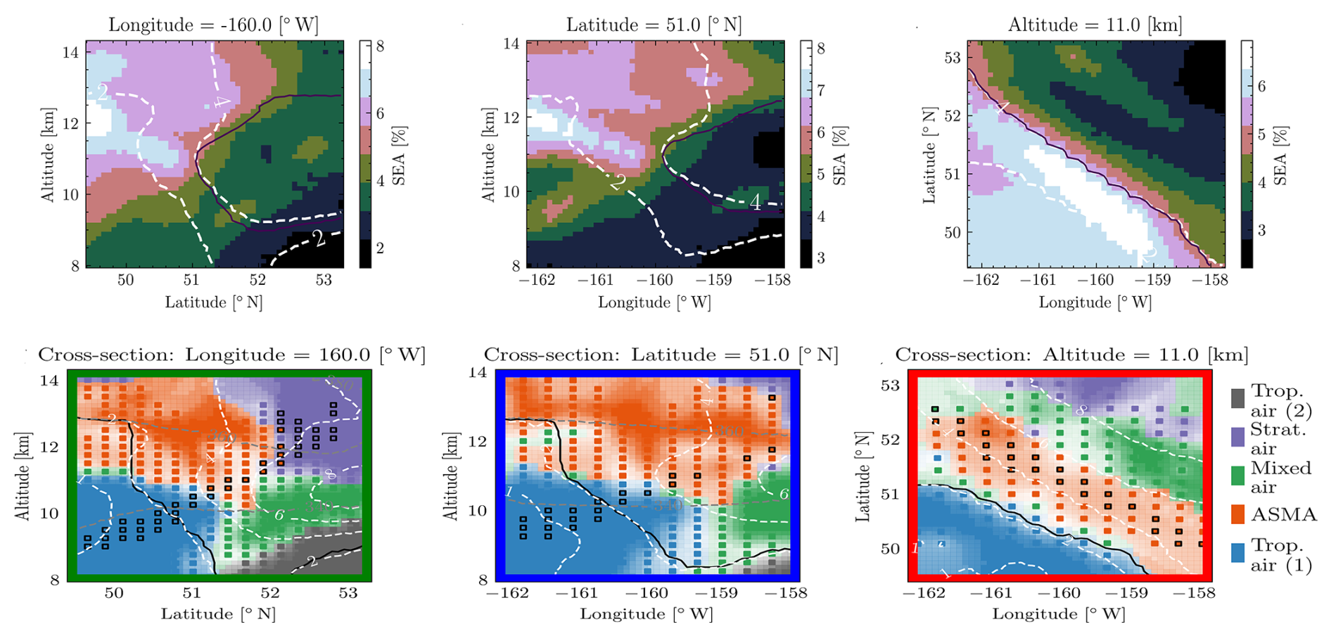
Figure B5 Comparison of SEA surface-origin tracers to the classification. The cross-sections shown are the same as in Fig. 5a–c.

B4 Comparison to conventional classification

The comparison between the BGMM classification and conventional methods is illustrated in Fig. B6. The tracers H₂O and O₃ have been chosen since most conventional methods use them. Any other combination of tracers will yield a more chaotic correlation. The BGMM classification is shown in Fig. B6a in color-code. The first conventional method used the tropopause similarly to Ungermann et al. (2016) to determine the tropospheric and stratospheric regimes. For either regime a linear regression if performed to determine the air types. Air parcels are included into either tropospheric/stratospheric regime if the regression suggests at least 66 % prediction confidence. The classification fails to provide complete classification for either tropospheric/stratospheric air, indicated by the green regimes above the stratospheric band and to the sides of the tropospheric band. Mixed air (in the form of mixing lines between the tropospheric/stratospheric band) is underrepresented compared to the other classifications. This classification would allow a total of four regimes to be defined (in either quadrant of the bands), but the section corresponding to the ASM air in Fig. B6a is generally not considered in this approach.

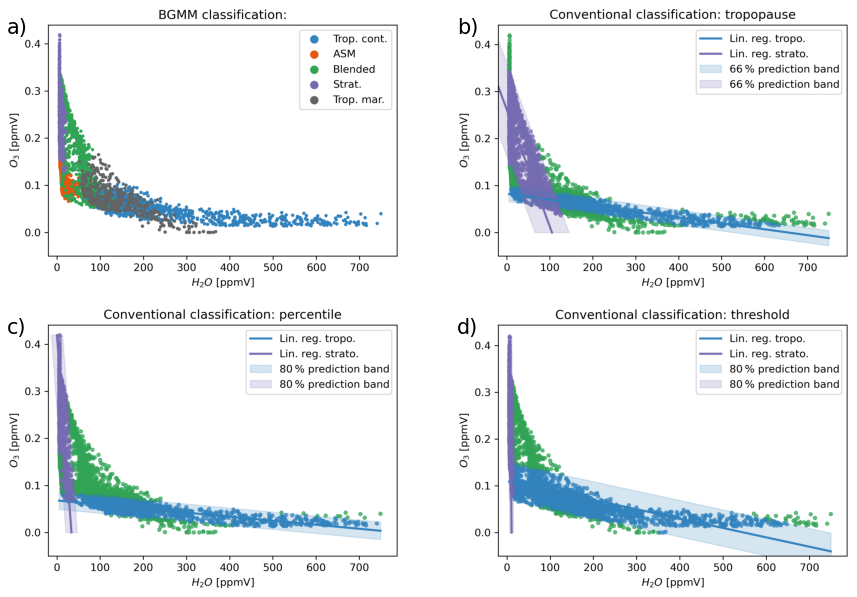
Figure B6 Comparison to conventional classification methods. (a) The BGMM classification presented in this study as a reference. (b) Classification based on the thermal tropopause. The tropospheric (blue), stratospheric (purple) and mixed (green) regimes are determined by linear regression based on the trace gas species H₂O and O₃ above and below the tropopause. (c) Classification based on thresholds determined by percentiles (80 %) of the measured data. (d) Classification based on commonly used thresholds. The conventional classifications include tropospheric air, stratospheric air and mixed air.

The second conventional approach uses percentile thresholds similarly to Cohen et al. (2023) to identify tropospheric/stratospheric air. Linear regressions through either regime are performed and the air parcels classified accordingly. This classification is most similar to the BGMM classification, but only yields three significant regions. The third conventional approach uses commonly used fixed thresholds similarly to Ma et al. (2022). We use a threshold of 20 ppmV H₂O for the tropospheric regime and a threshold of 0.2 ppmV O₃ and perform linear regressions. This classification yields a stratosphere most similar to Fig. B6a, and a reasonable definition of th troposphere. However, it is only capable of identifying three distinct regimes. Neither conventional method can reasonably perform a classification into more than three classes. Even between different conventional approaches significant differences persist.

B5 Robustness of BGMM parameters

An instance of a trained (converged) BGMM generally converges towards the same state. Small variability may be introduced by different initializations or ambiguity of the clusters contained with the data. To illustrate the robustness of the BGMM shown here an ensemble of 100 instances was trained and the variability of the BGMM parameters such as means (cluster centers) and covariances (cluster shapes) were determined. Figure B7 summarizes the results. The means of each cluster are indeed rather robust, with the largest variability found for H₂O and the continental tropospheric class (blue) in general. Since water vapor has the largest intrinsic variability this result is partially expected. The mixing weights (panel b) vary little, indicating indeed well defined clusters with sufficient local point density and global variability. The covariances also are subject to very little variability, with the most uncertainty found for the correlation between H₂O and HNO₃ in the blended class and the variance in H₂O in the maritime tropospheric class such that the cluster shape along these axes (and subsequently along the contributions of those axes to the principal components) may vary. The covariances shown here were calculated from the untransformed clusters (in 5-D) based on clusters found in the reduced 3-D space.

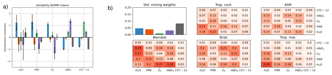
Figure B7 Robustness estimation for determined BGMM parameters. A total of 100 fits were performed and standard deviations of each parameter were determined. (a) Variability of the cluster centers. The standard deviation is shown as errorbar for each component of each cluster. (b) Variability of mixing weights (first plot) and the covariance matrices for each cluster. The scale of the standard deviations is indicated in color-code.