A WRF-Chem study of the greenhouse gas column and in situ surface mole fractions observed at Xianghe, China – Part 2: Sensitivity of carbon dioxide (CO₂) simulations to critical model parameters

Understanding the variability and sources of atmospheric CO₂ is essential for improving greenhouse gas monitoring and model performance. This study investigates temporal CO₂ variability at the Xianghe site in China, which hosts both remote sensed (TCCON-affiliated) and in situ (PICARRO) observations. Using the Weather Research and Forecast model coupled with Chemistry, in its greenhouse gas option (WRF-GHG), we performed a one-year simulation of surface and column-averaged CO₂ mole fractions, evaluated model performance and conducted sensitivity experiments to assess the influence of key model configuration choices. The model captured the temporal variability of column-averaged mole fraction of CO₂ (XCO₂) reasonably well (r=0.7), although a persistent bias in background values was found. A July 2019 heatwave case study further demonstrated the model’s ability to reproduce a synoptically driven anomaly. Near the surface, performance was good during afternoon hours (r=0.75, MBE =2.44 ppm), nighttime mole fractions were overestimated (MBE = 7.86 ppm), resulting in an exaggerated diurnal amplitude. Sensitivity tests revealed that land cover data, vertical emission profiles, and adjusted VPRM-parameters (Vegetation Photosynthesis and Respiration Model) can significantly influence modeled mole fractions, particularly at night. Tracer analysis identified industry and energy as dominant sources, while biospheric fluxes introduced seasonal variability – acting as a moderate sink in summer for XCO₂ and a net source in most months near the surface. These findings demonstrate the utility of WRF-GHG for interpreting temporal patterns and sectoral contributions to CO₂ variability at Xianghe, while emphasizing the importance of careful model configuration to ensure reliable simulations.

1 Introduction

Climate change is one of the most pressing global challenges, and carbon dioxide (CO₂) is its primary driver due to its long atmospheric lifetime and rising atmospheric abundance (Masson-Delmotte et al., 2021). Understanding how atmospheric CO₂ levels vary over time and space is essential for detecting long-term trends, distinguishing natural fluctuations from anthropogenic signals, and deepening our insight into the carbon cycle and its interactions with the atmosphere. Observational records are key to unraveling local and regional carbon budgets and assessing the effectiveness of mitigation strategies. To fully interpret such observations, especially in complex environments, we rely on atmospheric transport models, which provide spatial and temporal context and help disentangle the observed CO₂ signal into contributions from different sources and processes. As the world’s largest fossil CO₂ emitter (Friedlingstein et al., 2025), our study focuses on China – a country whose vast and densely populated regions, strong industrial activity, and ecological diversity make it a complex but highly relevant area for atmospheric CO₂ research. In this context, a ground-based remote sensing instrument was installed in 2018 at the Xianghe site, a suburban location approximately 50 km southeast of Beijing. The Fourier Transform Infrared (FTIR) spectrometer provides high-precision column-averaged CO₂ mole fractions and is part of the global Total Carbon Column Observing Network (TCCON). Complementing this, a PICARRO Cavity Ring-Down Spectroscopy (CRDS) analyzer measures near-surface CO₂ mole fractions at 60 m above ground level. This unique combination of collocated column and in situ observations – to our knowledge currently the only such setup in China – offers a valuable opportunity to study both local and regional CO₂ signals and to evaluate model performance for different levels of the atmosphere.

Previous studies by Yang et al. (2020, 2021) provided initial insights into the seasonal and diurnal variability of both column-averaged and near-surface CO₂ mole fractions at Xianghe. Their work highlighted the strong influence of local and regional emissions, as well as planetary boundary layer dynamics, on observed CO₂ levels. However, these analyses were either purely observational or relied on coarser-resolution model products such as CarbonTracker, which are limited in their ability to resolve mesoscale variability. Furthermore, the two observation types were not jointly analyzed within a high-resolution modeling framework, leaving room for a more detailed and integrated approach. To gain a deeper understanding of the processes shaping the observed CO₂ mole fractions at Xianghe, we apply the high-resolution WRF-GHG model in this work, a specific configuration of the widely used WRF-Chem model tailored for greenhouse gas simulations (Beck et al., 2011). The current study is part of a broader research effort investigating multiple greenhouse gases at the site. While a companion paper has already presented the results for CH₄ (Callewaert et al., 2025), the present work focuses exclusively on CO₂.

The WRF-GHG model was originally developed to address the limitations of coarse-resolution global models by providing a more detailed representation of CO₂ transport, surface flux exchanges, and meteorological processes at the mesoscale. Thanks to its coupling with the Vegetation Photosynthesis and Respiration Model (VPRM), WRF-GHG has demonstrated strong capabilities in simulating biogenic CO₂ fluxes (NEE, net ecosystem exchange) and atmospheric dynamics. It has been successfully applied across a range of environments, from rural areas influenced by sea-breeze circulations (Ahmadov et al., 2007, 2009, there referred to as WRF-VPRM) to urban regions with complex emission patterns and boundary layer processes (Feng et al., 2016; Park et al., 2018; Zhao et al., 2019). Further, the model has been evaluated against in situ, tower, aircraft and satellite data during large-scale campaigns such as ACT-America in the US (Hu et al., 2020) and KORUS-AQ in South-Korea (Park et al., 2020), showing its ability to reasonably capture spatiotemporal variability of CO₂. In China, WRF-GHG has been used to study CO₂ fluxes and atmospheric mole fractions on a national scale and to explore the role of biospheric and anthropogenic sources (Dong et al., 2021; Ballav et al., 2020). Li et al. (2020) evaluated WRF-GHG against tower observations in northeast China, showing the model could capture seasonal trends and episodic enhancements, despite underestimating diurnal variability and respiration fluxes.

Our study uses WRF-GHG to investigate the main drivers of observed temporal variations at Xianghe and to evaluate the model’s ability to reproduce these patterns, identifying key sources of error where relevant. The model’s tracer framework further allows us to disentangle the contributions of anthropogenic, biogenic, and meteorological processes to simulated CO₂ levels. The structure of the paper is as follows: Sect. 2 describes the observations, model configuration, and the design of additional model sensitivity experiments. Section 3 presents the results, including model performance, tracer-based analyses and sensitivity experiments. Section 4 discusses some of the results in more detail, while Sect. 5 summarizes the conclusions and provides an outlook.

2 Methods

2.1 Observations at Xianghe site

We use observational data from the atmospheric monitoring station situated in Xianghe county (39.7536° N, 116.96155° E; 30 m a.s.l.). This site is located in a suburban part of the Beijing-Tianjin-Hebei (BTH) region in northern China. The town center of Xianghe lies approximately 2 km to the east, while the major metropolitan areas of Beijing and Tianjin are situated roughly 50 km to the northwest and 70 km to the south-southeast, respectively (Fig. 1b). The dominant vegetation in the surrounding area consists of cropland.

Continuous atmospheric measurements have been conducted at the Xianghe observatory by the Institute of Atmospheric Physics (IAP), Chinese Academy of Sciences (CAS), since 1974. FTIR solar absorption measurements have been performed since June 2018, from the roof of the observatory by a Bruker IFS 125HR. This ground-based remote sensing instrument records spectra in the infrared range and is part of the TCCON network (Wunch et al., 2011; Zhou et al., 2022), providing data on total column-averaged dry air mole fractions for gases such as CO₂, CH₄, and CO (noted as XCO₂, XCH₄ and XCO, respectively). The current study employs the GGG2020 data product (Laughner et al., 2024). Observations are typically taken every 5 to 20 min, depending on weather conditions and instrument status. TCCON measurements are exclusively performed under clear skies. The uncertainty associated with the XCO₂ measurements is approximately 0.5 ppm. Further details regarding the instrument and the retrieval methodology can be found in Yang et al. (2020).

In addition to the FTIR measurements, in situ measurements of CO₂ and CH₄ mole fractions have been conducted since June 2018 using a PICARRO cavity ring-down spectroscopy G2301 analyzer. This instrument draws air from an inlet situated on a 60 m tower. A more comprehensive description of this measurement setup is available in Yang et al. (2021). The measurement uncertainty for CO₂ with this instrument is about 0.06 ppm. The data used in this study were converted to align with the WMO CO₂ X2019 scale (Hall et al., 2021).

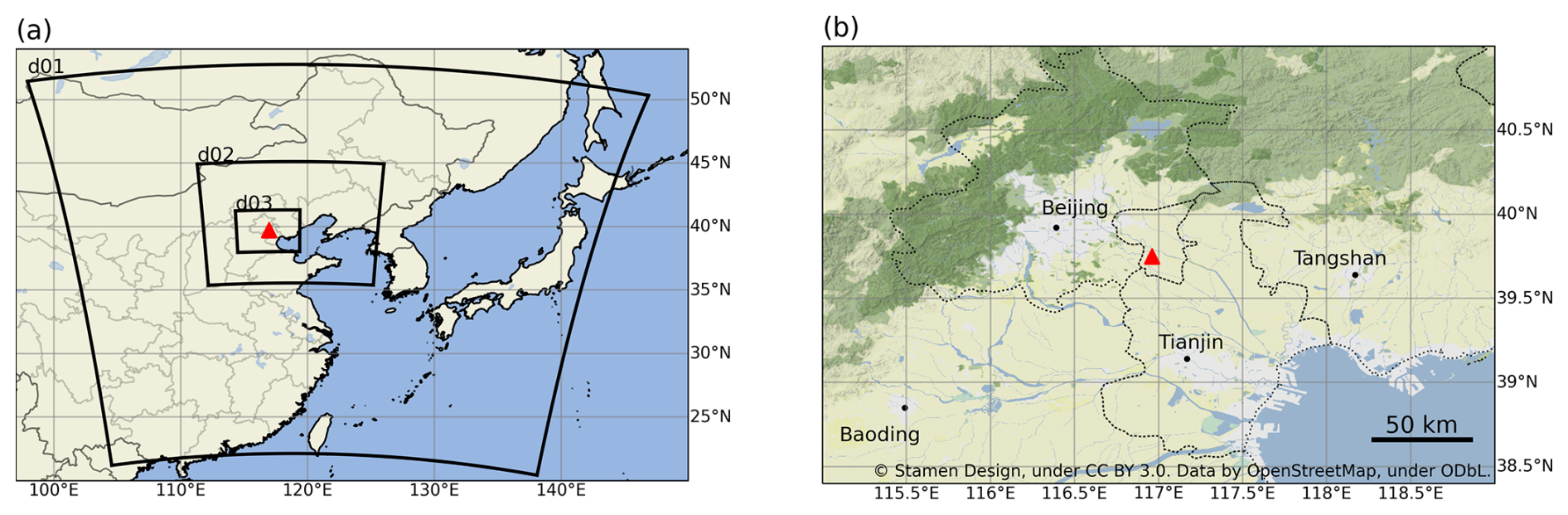
Figure 1 (a) Location of the WRF-GHG domains, with horizontal resolutions of 27 km (d01), 9 km (d02) and 3 km (d03). All domains have 60 (hybrid) vertical levels extending from the surface up to 50 hPa. (b) Terrain map including the largest cities in the region of Xianghe, roughly corresponding to d03. The location of the Xianghe site is indicated by the red triangle in both maps. Figure taken from Callewaert et al. (2025). ©OpenStreetMap.

2.2 WRF-GHG model simulations

We make use of the WRF-GHG model simulations elaborated in Part 1 of this work (Callewaert et al., 2025), and provide a brief summary here for completeness. The simulations were performed using the Weather Research and Forecasting model with Chemistry (WRF-Chem v4.1.5; Grell et al., 2005; Skamarock et al., 2019; Fast et al., 2006) in its greenhouse gas configuration, called WRF-GHG (Beck et al., 2011). This Eulerian transport model simulates three-dimensional greenhouse gas mole fractions simultaneously with meteorological fields, without accounting for chemical reactions. The model setup includes three nested domains with horizontal resolutions of 27, 9, and 3 km (Fig. 1a), and 60 vertical levels extending from the surface up to 50 hPa. There are 11 layers in the lowest 2 km, with a layer thickness ranging from about 50 m near the surface, to 400 m above 2 km.

Anthropogenic CO₂ emissions were obtained from CAMS-GLOB-ANT v5.3 (Granier et al., 2019; Soulie et al., 2024) and temporally disaggregated using CAMS-TEMPO profiles (Guevara et al., 2021). The original 11 source sectors were aggregated into four broader categories and included in separate tracers: energy, industry, transportation, and residential & waste. Biomass burning emissions were taken from the FINN v2.5 inventory (Wiedinmyer et al., 2011), and ocean-atmosphere CO₂ fluxes were prescribed based on the climatology from Landschützer et al. (2017). Finally, net biogenic CO₂ fluxes were calculated online using VPRM (Mahadevan et al., 2008; Ahmadov et al., 2007), driven by WRF-GHG meteorology and MODIS surface reflectance data, with ecosystem-specific VPRM parameters from Li et al. (2020) and land cover information from SYNMAP (Jung et al., 2006). Meteorological fields (e.g., wind, temperature, humidity) were driven by hourly data from the European Centre for Medium-Range Weather Forecasts (ECMWF) ERA5 hourly data (0.25° × 0.25°; Hersbach et al., 2023a, b). Daily restarts were performed at 00:00 UTC, with model initialization at 18:00 UTC the day before to allow for a 6-h spin-up, stabilizing the simulation. For tracer fields, mole fractions at 00:00 UTC were copied from the previous day’s simulation to maintain consistency. The initial and lateral boundary conditions for CO₂ were prescribed using the 3-hourly Copernicus Atmosphere Monitoring Service (CAMS) global reanalysis (EGG4, Agustí-Panareda et al., 2023).

The final simulated CO₂ field is composed of the sum of several tracers that track contributions from individual sources. These include a background tracer (reflecting the evolution of initial and lateral boundary conditions from CAMS), as well as tracers for energy, industry, residential, transportation, ocean, biomass burning, and biogenic fluxes.

WRF-GHG was run from 15 August 2018 to 1 September 2019. However, the first two weeks were regarded as a spin-up phase, so the analysis in Sect. 3.1 is made on one full year of data: from 1 September 2018 until 1 September 2019. The complete data set can be accessed on https://doi.org/10.18758/P34WJEW2 (Callewaert, 2023).

To enable comparison with the observations, model data from the grid cell containing the measurement site are extracted. For near-surface observations, the model profile is interpolated to the altitude of the instrument, while for column measurements the model output is smoothed with the FTIR retrieval’s a priori profile and averaging kernel, after being extended above the model top with the FTIR a priori profile. The hourly model output represents instantaneous values, as do the observational measurements. To align the datasets temporally, the observations are averaged around each model output time step – using a ±15-min window. Further details are provided in Part 1 (Callewaert et al., 2025).

2.3 Sensitivity experiment design

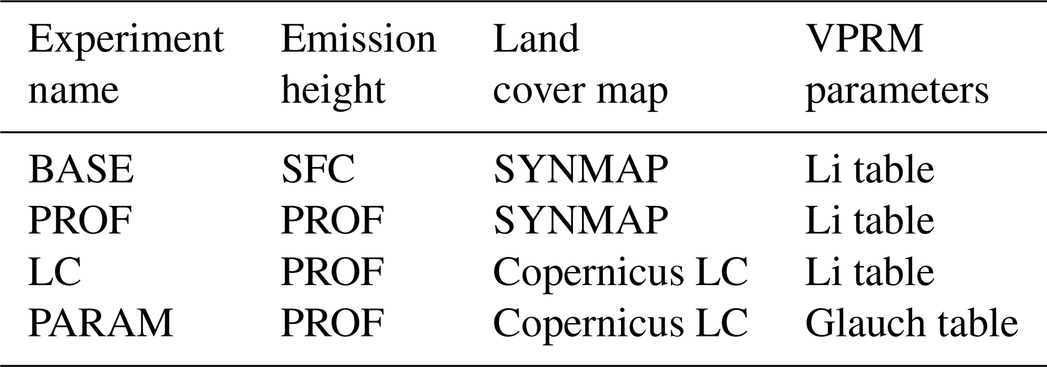
A series of sensitivity experiments was conducted to assess the impact of key model assumptions on surface CO₂ fluxes, such as the treatment of emission heights, land cover classification, and biogenic flux parameterizations. Four two-week periods were selected for these sensitivity simulations, spanning from the 15–29 March, May, July, and December. These months were identified as being most critical for simulating the diurnal CO₂ cycle while representing different seasons. Although the specific dates within each month (15–29) were chosen somewhat arbitrarily, they were applied consistently across all four months to ensure comparability. Four different simulation experiments (BASE, PROF, LC, PARAM) were performed over these four periods to isolate the impact of three model assumptions (see Table 1):

• Emission height. To assess the impact on simulated in situ CO₂ mole fractions at Xianghe of the height at which anthropogenic emissions are released in the atmosphere (all at the lowest model level near the surface, or according to sector-specific vertical profiles), we applied the vertical profiles for point sources from Brunner et al. (2019) to the CAMS-GLOB-ANT sector-specific CO₂ emissions. For the fluxes in the 'industrial processes' sector, we used the average of the profiles of SNAP 3 (Combustion in manufacturing industry) and SNAP 4 (Production processes). Note that we do not make a distinction between area and point sources as in Brunner et al. (2019), as this information is not available for our study region. Profile emissions were included in all but the BASE experiment: PROF, LC and PARAM.

• Land cover classification. The net biogenic CO₂ fluxes are calculated online in WRF-GHG as the weighted average of the Net Ecosystem Exchange (NEE) for eight vegetation classes (evergreen trees, deciduous trees, mixed trees, shrubland, savanna, cropland, grassland and non-vegetated land) (Mahadevan et al., 2008). As a default, the SYNMAP land cover map is used to calculate the vegetation fraction for every model grid cell. To assess the impact of this classification, we prepare the VPRM model input files for the LC and PARAM experiments with the global 100-m Copernicus Dynamic Land Cover Collection 3 (epoch 2019) (Buchhorn et al., 2020), using the pyVPRM python package (Glauch et al., 2025), allowing for an updated and higher-resolution representation of vegetation types in the domain.

• VPRM parameterization. The VPRM-calculated NEE can be tuned for different regions around the globe by specifying four empirical parameters (α, β, λ and PAR₀) per vegetation class. These parameter tables are a mandatory input to the WRF-GHG model and can be calibrated using a network of eddy flux tower sites, representing the different vegetation classes in the region, or taken from literature. Due to the lack of a dedicated calibration study in China, we applied the table from Li et al. (2020) in the one-year simulations, and the BASE and LC experiments. Seo et al. (2024) reported the lowest RMSE in East Asia using these parameter values, relative to the default US settings and those of Dayalu et al. (2018). To evaluate the impact of these parameters at Xianghe, we conducted an experiment (PARAM) with an alternative parameter table, optimized over Europe by Glauch et al. (2025). The exact parameter values used in each experiment are provided in Table A1.

Table 1 Overview of the model configuration for the sensitivity experiments. Note that the Glauch parameter table does not include values for the “Savanna” class, consistent with its absence in the Copernicus land cover map.

By comparing the results from the four sensitivity experiments, the influence of individual model components can be isolated. The role of vertical emission distribution can be assessed by comparing the BASE and PROF experiments. Similarly, the impact of land cover classification is assessed by comparing the PROF and LC simulations, which differ only in the land cover dataset used. Finally, the effect of VPRM parameterization can be evaluated by comparing LC and PARAM, which share the same land cover input but differ in the VPRM parameter table. This approach enables a systematic investigation of potential model deficiencies affecting the representation of CO₂ at Xianghe. Note that the BASE experiment corresponds exactly with the settings of the one-year simulation described above.

3 Results

3.1 Evaluation of one-year simulation

3.1.1 Timeseries and statistical comparison

Table 2 summarizes the comparison between simulated and observed CO₂ mole fractions at Xianghe. Overall, WRF-GHG demonstrates a reasonable accuracy in replicating these measurements: the XCO₂ observations are slightly underestimated, with a mean bias error of −1.43 (±1.99) ppm and a Pearson correlation coefficient of 0.70. Note that the XCO₂ time series was de-seasonalized before calculating the correlation coefficient in order to remove the effect of the seasonal variation. After applying a bias correction to the modeled values, the XCO₂ MBE decreases to −0.86 (±1.57) ppm (corrected values shown in parentheses in Table 2), and the RMSE improves from 2.45 to 1.80 ppm, while the correlation remains unchanged. Details of the bias correction are provided in Sect. 3.1.2, and the resulting time series are shown in Fig. 2 (and Fig. A1).

Table 2 Statistics of the model-data comparison of the ground-based CO₂ observations at the Xianghe site from 1 September 2018 until 1 September 2019. We present the mean bias error (MBE), root mean square error (RMSE) and Pearson correlation coefficient (CORR). The MBE and RMSE are given in ppm. For in situ observations, the data is split in afternoon (12:00–15:00 LT), night (22:00–04:00 LT) and morning transition (08:00–12:00 LT) hours. The bias corrected model values are given between brackets.

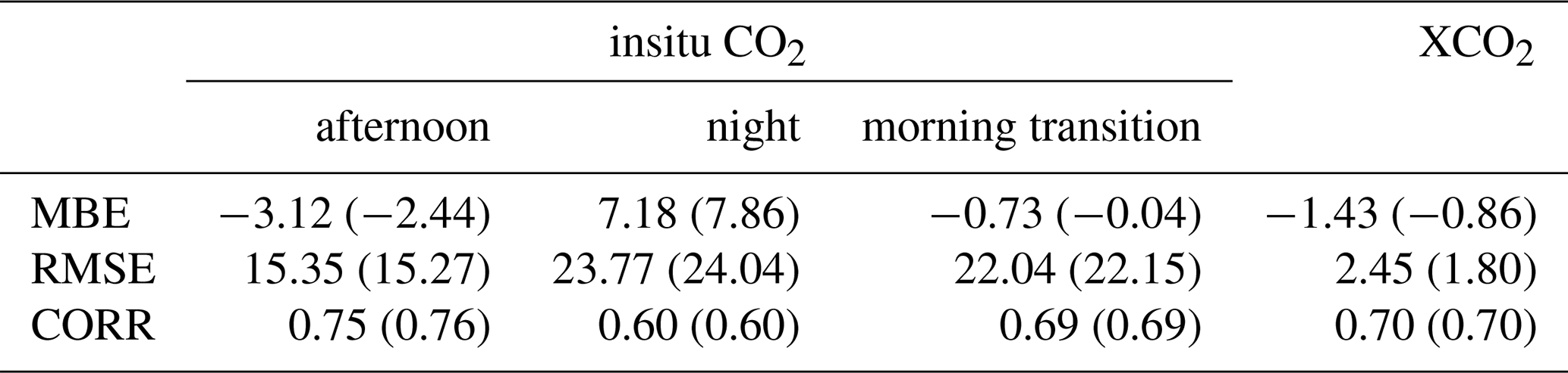
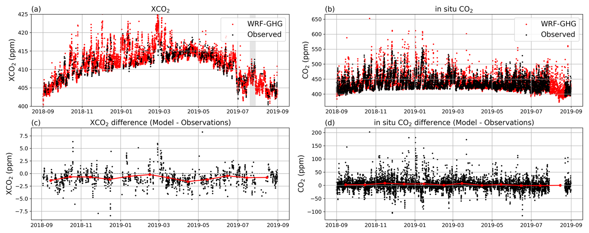
Figure 2 Time series of the observed (black) and simulated (red) (a) XCO₂ and (b) insitu CO₂ mole fractions at the Xianghe site. Panels (c) and (d) show the differences between (smoothed) WRF-GHG simulations and observations for XCO₂ and in situ CO₂, respectively. Data points are hourly, if available. The red data points in (b) and (d) represent the monthly mean differences. A bias correction was applied to the WRF-GHG values.

The data near the surface has been divided into afternoon (12:00–15:00 LT), nighttime (22:00–04:00 LT) and morning (08:00–12:00 LT) periods to assess model performance under different boundary layer conditions. Indeed, WRF-GHG shows a smaller bias (−2.44 ppm) during the afternoon, when the lower atmosphere is well-mixed, compared to nighttime (7.86 ppm). Additionally, the MBE differs in sign between the two periods: near-surface CO₂ levels tend to be underestimated by the model in the afternoon but overestimated at night. Except for the moderate correlation observed for in situ CO₂ during nighttime (0.60), WRF-GHG achieves relatively high correlation coefficients (≥0.7) for other CO₂ data, indicating satisfactory model performance. Overall, the bias correction has only a minor influence on the comparison with near-surface mole fractions, where the effect on RMSE and correlation coefficients are negligible (<1.2 % and <0.01, respectively).

Finally, the XCO₂ time series in Fig. 2a reveals a notable spike between 20–29 July (highlighted in gray), interrupting the general decline associated with northern hemispheric photosynthetic uptake during the growing season, from May onwards. A dedicated analysis of this July XCO₂ event is provided in Sect. 4.2. Note that there is a gap in the in situ CO₂ time series during this period due to instrument malfunctions (Yang et al., 2021).

3.1.2 Correction of background bias

Our WRF-GHG simulations underestimate XCO₂ by approximately 2 ppm until May 2019, after which the negative bias diminishes (see Fig. A1a, c). This bias likely originates from a similar error in the background data, inaccuracies in representing the actual sources and sinks in the region, or a combination of both.

The CAMS validation report (Ramonet et al., 2021) presents “a very good agreement for all (TCCON) sites”, suggesting that the CAMS reanalysis that is driving the WRF-GHG simulations is of good quality without known biases. However, their criteria for what constitutes “very good” appears to be relatively mild (within ±2 ppm). Moreover, the Xianghe site was not included in this report and the accompanying figure does not provide very detailed information. Therefore, we reproduced their analysis for several TCCON sites at similar latitudes for the period of our interest (September 2018–September 2019): Karlsruhe (49.1° N), Orleans (48.0° N), Garmisch (47.5° N), Park Falls (45.9° N), Rikubetsu (43.5^∘ N), Lamont (36.6^∘ N), Tsukuba (36.0° N), Edwards (35.0° N), Pasadena (34.1° N), Saga (33.2° N), and Hefei (31.9° N). The results of this analysis are presented in Fig. 3.

We find an underestimation of the CAMS reanalysis XCO₂ at all TCCON sites between 30–50° N (except Pasadena) from October 2018 until May 2019. More specifically for Xianghe, monthly mean errors range from −2.20 (±1.3) ppm in January 2019 to 3.38 (±1.28) ppm in July 2019, which is of a similar magnitude as the bias found with WRF-GHG (where the monthly mean differences with respect to the TCCON site of Xianghe range from −2.53 (±1.7) ppm in December 2018 to 1.28 (±1.57) ppm in July 2019).

Therefore, we assume that the error pattern detected in the XCO₂ time series is primarily the result of the same pattern in the background information. Moreover, this bias pattern is not found in the in situ CO₂ time series, likely because the relative contribution from the background to the in situ mole fractions is smaller than it is to the column data.

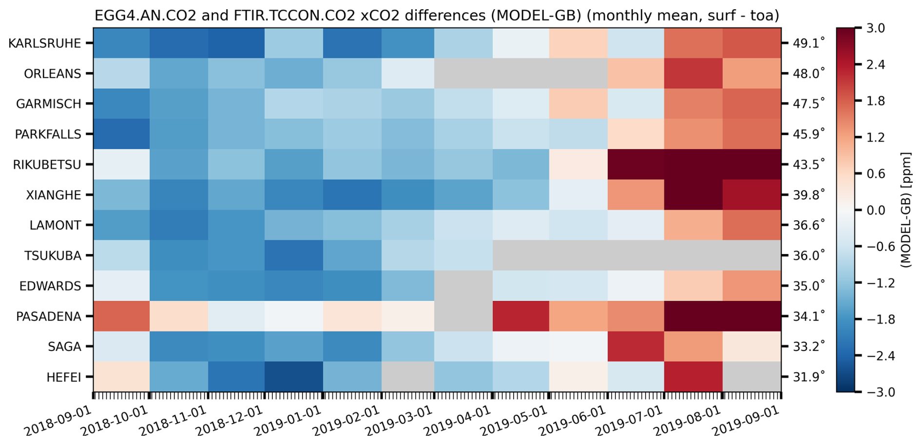
Figure 3 Monthly mean difference (in ppm) between CAMS reanalysis model and TCCON XCO₂ between 30–50° N over the simulation period of this study.

To account for the systematic bias introduced by the background values, we applied a bias correction to the WRF-GHG simulations. Specifically, we subtract the monthly mean difference between CAMS and TCCON XCO₂, averaged across all TCCON sites located between 30–50° N (excluding Pasadena due to outlier behavior), from the model’s background tracer. The resulting improvements in model performance are summarized in Table 2 between parentheses.

3.2 Sector contributions to observed mole fractions

WRF-GHG tracks all fluxes in separate tracers, enabling the decomposition of the total simulated CO₂ mole fractions at Xianghe into contributions from different source sectors. Figure 4 shows the monthly mean values, while additionally the median and interquartile ranges are presented in Table 3. Note that all simulated hours were used for this analysis, not just the ones coinciding with observations.

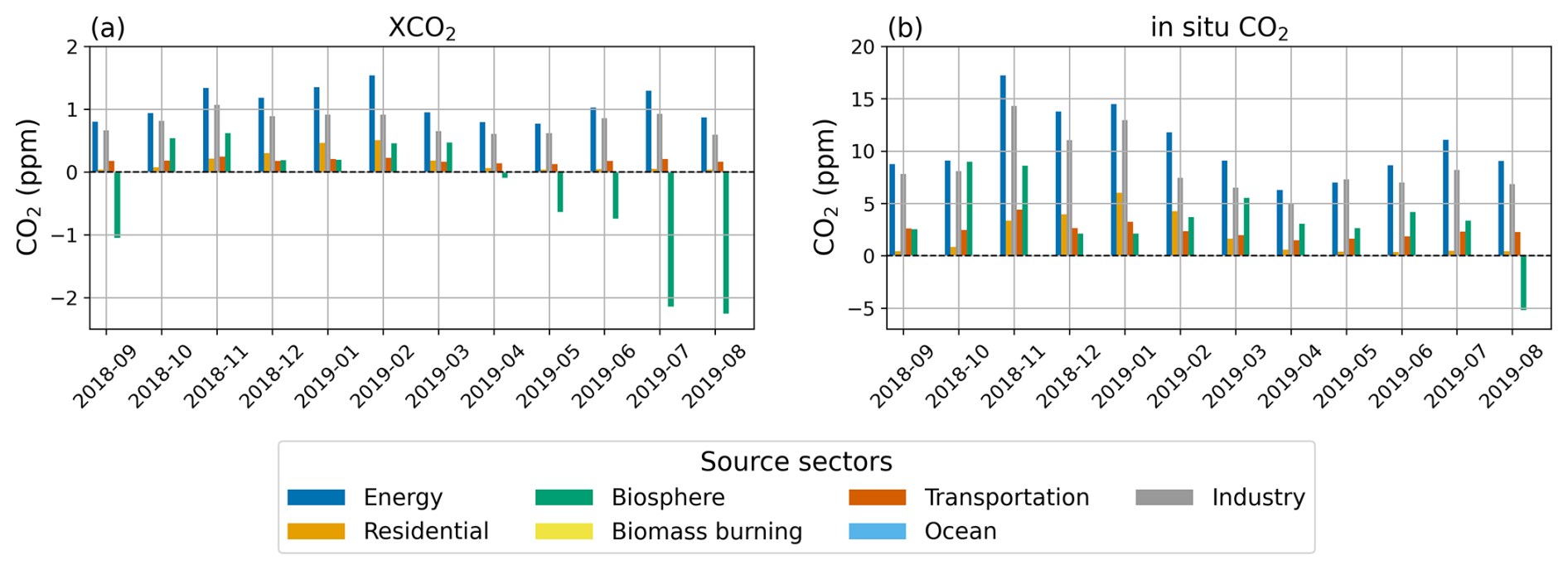
Figure 4 Monthly mean tracer contributions above the background for (a) XCO₂ and (b) in situ CO₂ simulated mole fractions at Xianghe.

Table 3 Statistics of the total simulated CO₂ mole fractions and the different tracer contributions over the complete simulation period. Q1 and Q3 represent the first and third quartile, respectively, between which 50 % of the data fall.

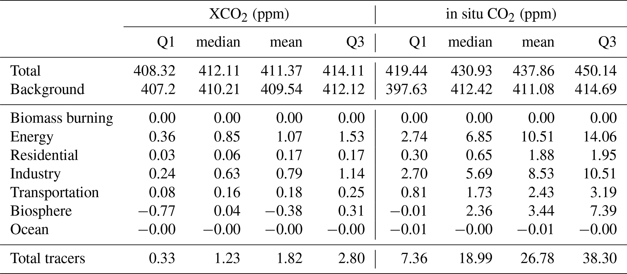
The main sectors contributing to the modeled CO₂ variability at Xianghe are energy, industry, and the biosphere. For XCO₂, we find median values of 0.85 and 0.63 ppm for the energy and industry sectors, respectively. Furthermore, the biosphere significantly influences the column-averaged CO₂ values, where it acts as a sink from April to September with a median value of −0.77 ppm during this period. During the rest of the year, the biogenic tracer acts as a small source (median value of 0.22 ppm).

Near the surface, median enhancements of in situ CO₂ mole fractions are 6.85 and 5.69 ppm for the energy and industry sectors, respectively. The biosphere generally acts as a source throughout the year, with a median contribution of 2.69 ppm, except in August, when it becomes a significant sink of −6.76 ppm.

Next to the three dominant sectors (biosphere, industry, and energy), transportation and also residential sources have a smaller but still relevant influence on the Xianghe data. During winter, the contribution of residential sources increases, where the highest values for the column simulations are found in February (median of 0.45 ppm) while near the surface this occurs in January (4.28 ppm). This peak aligns with heightened residential emissions in winter, driven by increased heating demands correlated with air temperature (Guevara et al., 2021). Finally, no relevant impact was found from biomass burning and the ocean. Overall, the total tracer enhancement for the in situ mole fractions is about ten times greater than that of the column-averaged values.

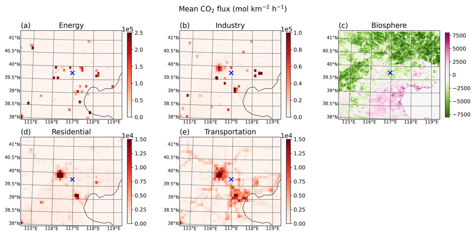
Figure 5 Map of the mean CO₂ flux (mol km⁻² h⁻¹) in WRF-GHG domain d03 during the entire simulation period from September 2018 until September 2019, for the most important sectors. Remark that the panels have different color scales. The location of the Xianghe site is indicated by a blue cross.

3.3 Diurnal cycle analysis of in situ data

The planetary boundary layer (PBL) plays a crucial role in regulating near-surface CO₂ mole fractions. Figure 6 displays the diurnal variation of the PBL height as simulated by WRF-GHG, along with the corresponding CO₂ mole fractions near the surface (both simulated and observed).

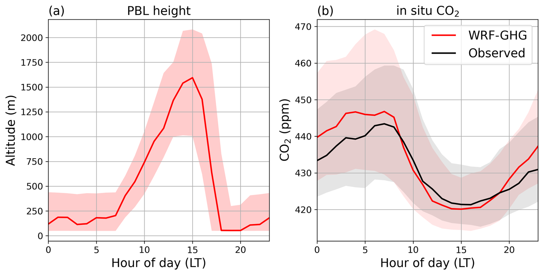
Figure 6 Hourly median and interquartile range of the (a) simulated planetary boundary layer height, and observed and simulated surface (b) CO₂ mole fraction at Xianghe.

During the day, solar radiation promotes turbulent mixing, leading to a deepening of the PBL and the dilution of near-surface CO₂. The PBL reaches its maximum height around 15:00 local time (LT), coinciding with the lowest surface CO₂ mole fractions. Conversely, during the night, radiative cooling leads to the formation of a stable, shallow PBL, trapping CO₂ near the surface and causing mole fractions to rise. As the sun rises and the PBL height begins to increase again, the CO₂ mole fractions drop, giving rise to a characteristic diurnal cycle.

Indeed, the lowest values are observed between 14:00 and 16:00 LT, with a minimum of 421.32 (hourly median value, with an interquartile range of 415.80–431.76) ppm at 16:00 LT. In the early morning, the observed CO₂ mole fractions show a distinct peak at 07:00 LT, reaching 443.42 (428.00–459.32) ppm. WRF-GHG successfully captures the general shape of this diurnal cycle, but discrepancies remain in the amplitude and timing. The model slightly underestimates daytime mole fractions, with a minimum value that is 1.22 ppm lower and occurs one hour earlier than the observations (at 15:00 LT). The peak CO₂ mole fractions in WRF-GHG are also reached at 07:00 LT, but overestimated by 3.36 ppm. Furthermore, this peak is less distinct as in the observations, where the model remains relatively stable between 03:00 and 08:00 LT. This results in an overestimation of the diurnal amplitude by approximately 4.58 ppm. Such a nighttime overestimation was not observed for CH₄ at the same site (Callewaert et al., 2025), suggesting that the bias is more likely related to the surface fluxes of CO₂ than to PBL dynamics.

3.4 Sensitivity experiments

Several sources of uncertainty may affect the accuracy of the simulated anthropogenic CO₂ fluxes and NEE in WRF-GHG. First of all, the parameters used in VPRM in this study are based on Li et al. (2020), who optimized them for ecosystems in the United States. Applying these values to China likely introduces regional mismatches, as differences in dominant species, climate conditions, and land use history can significantly alter ecosystem carbon dynamics even within the same vegetation class (Mahadevan et al., 2008; Seo et al., 2024). Moreover, the linear formulation of the respiration term in VPRM has been identified as a source of potential bias (Dong et al., 2021; Hu et al., 2021). A third concern is the land cover classification. VPRM uses the SYNMAP product (Jung et al., 2006), which is a 1-km global land cover map that classifies the area around Xianghe as 100 % cropland. While broadly consistent with the regional land use, this dataset does not account for increasing urbanization during the last decades. In WRF-GHG, built-up areas are assigned zero NEE, so their omission could contribute to the observed nighttime overestimation of respiration and daytime photosynthetic uptake.

Further, the representation of anthropogenic emission heights may also affect the modeled surface mole fractions. In this study, all anthropogenic CO₂ emissions are released in the lowest model layer, which simplifies reality. Especially for sectors such as energy and industry, this is a crude approximation, since facilities like power plants typically emit at elevated stacks. Previous work by Brunner et al. (2019) has shown that ignoring the vertical distribution of emissions can lead to overestimation of near-surface mole fractions.

Finally, while it is well known that uncertainties in simulating planetary boundary layer (PBL) dynamics can substantially affect near-surface CO₂ mole fractions, the influence of different PBL parameterization schemes is not explored in the current sensitivity experiments. WRF-GHG offers several PBL schemes, some of which were tested and discussed in Part 1 of this work (Callewaert et al., 2025). Here, the focus is instead on evaluating how model configuration choices related to CO₂ fluxes impact the simulated mole fractions.

3.4.1 Emission height sensitivity

To evaluate the impact of emission injection height on simulated CO₂ mole fractions at Xianghe, we compare the BASE and PROF sensitivity experiments (see Sect. 2.3). Figure 7 presents the median diurnal cycle of the anthropogenic CO₂ tracer across the four 14-d simulation periods (top), together with the total simulated and observed CO₂ mole fractions (bottom). Similarly, Table 4 provides a summary of the impact on the anthropogenic tracer.

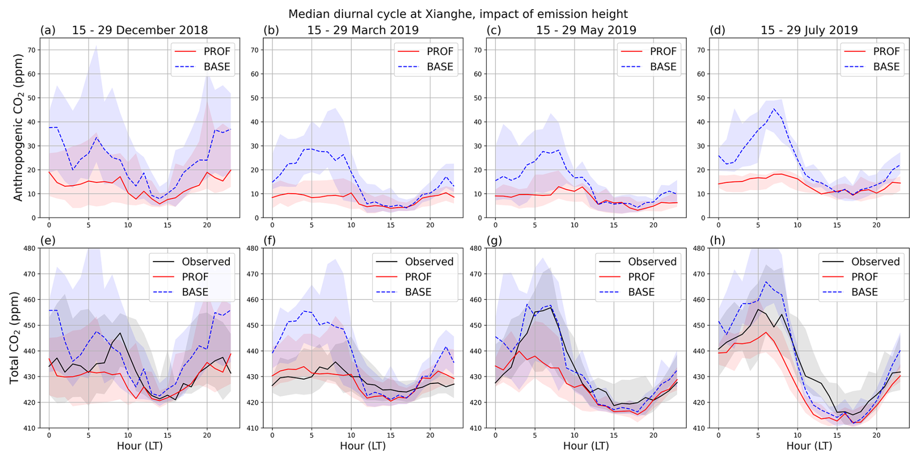
Figure 7 Median diurnal cycle of in situ CO₂ mole fractions (ppm) at Xianghe. The solid red line presents the simulated values of the PROF sensitivity experiment (using vertical profiles for the anthropogenic emissions), while the dashed blue line represents the simulated CO₂ values using only surface emissions (SFC). Observations are plotted in black.

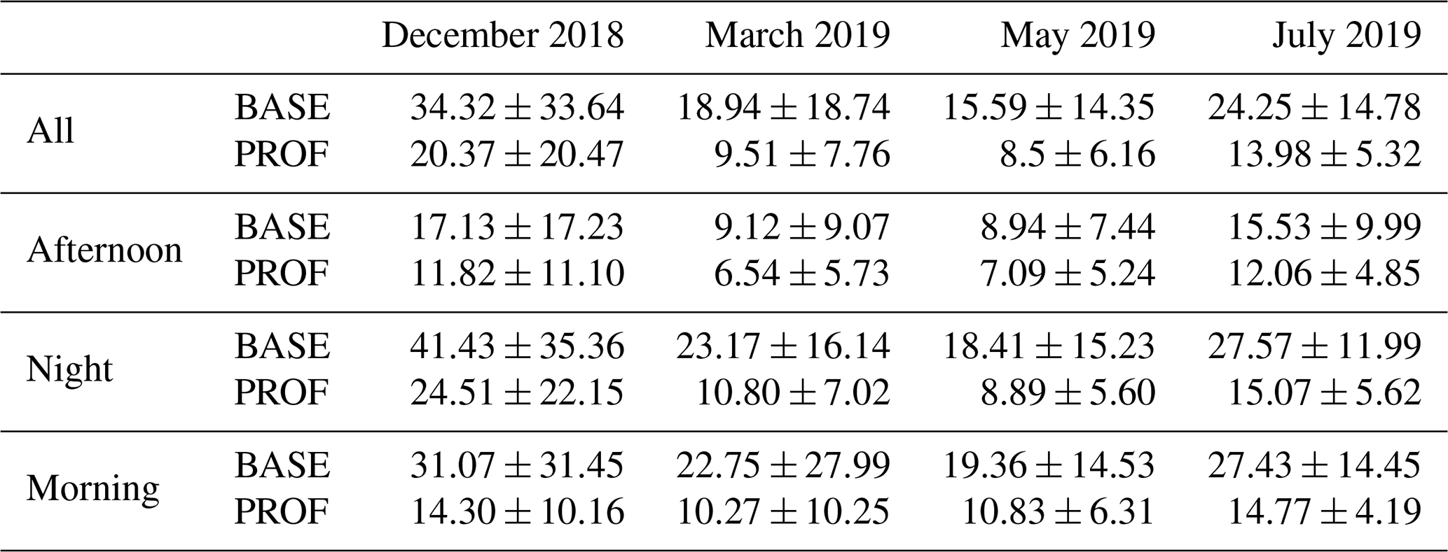
Table 4 Mean and standard deviation (in ppm) of the total anthropogenic CO₂ tracer contribution (sum of industry, energy, transportation and residential tracer) to near-surface mole fractions at Xianghe for the BASE and PROF sensitivity experiments, and simulation period. “All” indicates that all simulated hours (00:00–23:00 LT) were used to calculate the metrics, in contrast to “Afternoon” (12:00–15:00 LT), “Night” (22:00–04:00 LT) and “Morning” (08:00–12:00 LT).

Simulations using elevated emission profiles (PROF) consistently yield lower near-surface CO₂ mole fractions than those with surface-only emissions (BASE), with the most pronounced differences occurring during nighttime and the morning transition. The largest reduction is observed in December, where mean nighttime mole fractions in the PROF simulation are 16.92 ppm lower than in BASE.

Table 5 Overview of statistical metrics (MBE, RMSE and CORR) for the different sensitivity experiments BASE, PROF, LC and PARAM with respect to the observations, per simulation period. Values for MBE and RMSE are given in ppm.

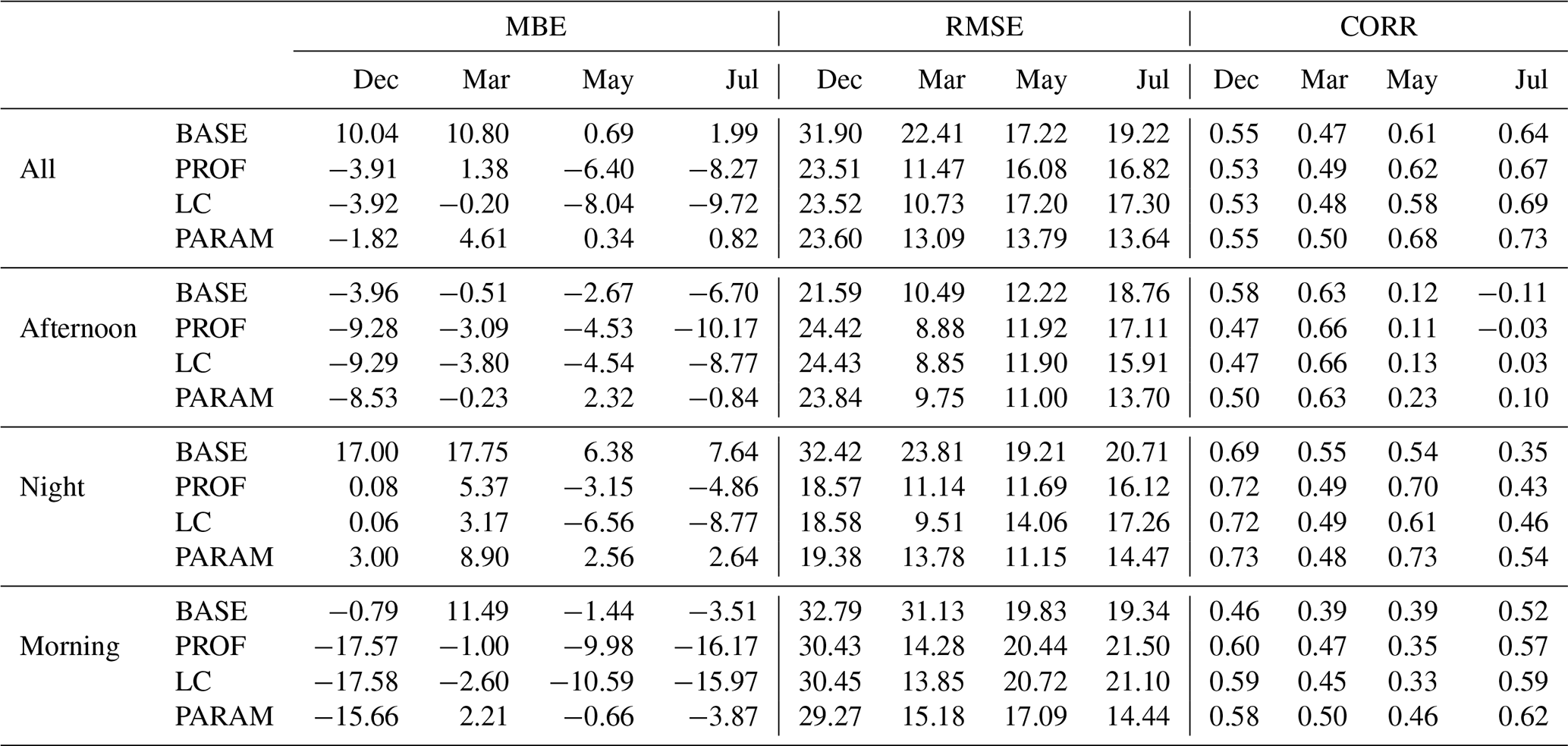
An overview of the key statistical performance metrics with respect to the observations at Xianghe is given in Table 5. In December and March, BASE shows large positive mean biases (MBE), primarily driven by nighttime overestimation; this bias is substantially reduced in PROF. By contrast, in May and July the absolute MBE increases and changes sign from positive to negative. The use of elevated emissions leads to a reduction in the RMSE compared to the surface-only configuration in all periods, while the correlation coefficient remains largely unaffected. The use of elevated emission profiles also has a pronounced effect on the simulated diurnal amplitude of near-surface CO₂. Compared to the surface-only configuration, which strongly overestimates the amplitude, the more realistic vertical distribution results in a better agreement with observations – particularly in March and July. In March, for example, the amplitude overestimation is reduced from 22.73 ppm to just 1.74 ppm, and in July from 14.16 to −5.96 ppm. The implementation of elevated anthropogenic emissions has a minimal effect on the column-averaged XCO₂ mole fractions at Xianghe, see statistical metrics in Table A2.

3.4.2 Biogenic flux and land cover sensitivity

To evaluate the impact of land cover representation on the VPRM-calculated CO₂ fluxes, we compare the PROF and LC sensitivity experiments. In the PROF simulation, the WRF-GHG grid cell containing the Xianghe site is classified as 100 % cropland using the SYNMAP dataset. In contrast, the Copernicus Dynamic Land Cover data, used in the LC experiment, classifies the same cell as 68.88 % cropland, 23.5 % no vegetation (representing urban surfaces, water, ice, rocks, etc.), 3.45 % mixed forest, 2.03 % wetland, 1.5 % shrubland, and 0.64 % grassland. A comparison of the two land cover datasets over the innermost WRF-GHG domain (d03) is shown in Fig. A4. Due to its higher spatial resolution and more up-to-date information, the Copernicus dataset introduces more heterogeneous vegetation fractions and especially reduces the cropland fraction while increasing the urban land category compared to SYNMAP.

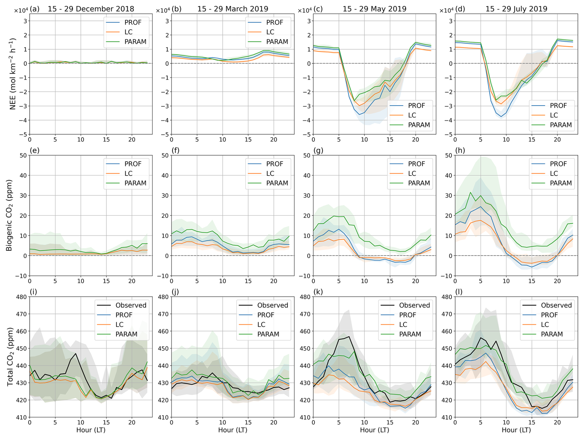
Figure 8 Median diurnal cycle of NEE (a–d), biogenic CO₂ tracer contribution (e–h) to the near surface CO₂ mole fractions (i–l) at Xianghe for the different simulation periods (columns). Different curves (colors) represent different sensitivity experiments PROF, LC and PARAM. Observations are plotted in black in the bottom row.

Table 6 Mean and standard deviation of the biogenic CO₂ tracer at Xianghe for the different sensitivity experiments BASE, LC and PARAM, per simulation period. “All” indicates all simulated hours (00:00–23:00 LT) were used to calculate the metrics, in contrast to “Afternoon” (12:00–15:00 LT), “Night” (22:00–04:00 LT), and “Morning” (08:00–12:00 LT).

The top panels of Fig. 8 present the median diurnal cycles of NEE, at Xianghe across the four 14-d simulation periods. Differences between the experiments are negligible in winter months (December and March), whereas during May and July, the LC simulation exhibits both reduced daytime CO₂ uptake and lower nighttime respiration compared to PROF. This change in NEE is reflected in the simulated biogenic CO₂ tracer at Xianghe (Fig. 8e–h, Table 6). However, we notice that the magnitude of the difference between LC and PROF is more pronounced at night. For instance, in July, the mean (± standard deviation) difference in the biogenic tracer is −3.91 (±2.13) ppm during nighttime, while the daytime difference is only −1.41 (±1.26) ppm.

To assess the impact of the VPRM parameterization on CO₂ simulations at Xianghe, we compare the LC and PARAM experiments. Both simulations use the 100-m Copernicus Dynamic Land Cover dataset but differ in their VPRM parameter tables (see Table 1). The comparison reveals that PARAM systematically produces more positive NEE than LC, both during daytime and nighttime. The change in NEE is reflected in the biogenic CO₂ tracer mole fractions at Xianghe. In July, for example, tracer values in PARAM are on average 10.61 (±5.03) ppm higher than in LC. This difference is again more pronounced at night (11.48 ± 4.27 ppm) than during the afternoon (8.01 ± 3.09 ppm).

A summary of the model performance of the different experiments is shown in Table 5. Generally, the PARAM experiment yields the best agreement with observations. Across all months, PARAM shows the highest correlation coefficients and the lowest MBE and RMSE, with the exception of March. In that month, the LC experiment outperforms PARAM, with a smaller MBE (−0.2 ppm vs. 4.61 ppm) and RMSE (10.73 ppm vs. 13.09 ppm).

The various VPRM inputs have only a minor influence on the column-averaged XCO₂ mole fractions at Xianghe, as indicated by the statistical metrics in Table A2.

4 Discussion

4.1 Sector contributions: differences between in situ CO₂ and XCO₂

In Sect. 3.2 we compared relative tracer contributions in the WRF-GHG simulations for near-surface CO₂ and column-averaged XCO₂, and found a notable difference in the biogenic contribution between the two. To analyze this difference, Fig. 9 presents mean vertical profiles of the simulated CO₂ tracers at Xianghe.

The profiles show that the dominant tracer signals in WRF-GHG are limited to the lowest 4 km of the column. Panel (a) reveals a large monthly variability in the vertical distribution of the biogenic tracer. From May through September the biogenic signal at Xianghe is generally negative through much of the column but positive in the lowest levels. Near-surface values (below 200 m) are, on average, positive in all months except August. This pattern is consistent with Fig. 4, which shows a negative biosphere contribution in August for in situ CO₂ while XCO₂ indicates a biospheric sink across May–September. These vertical profiles indicate that the difference can be linked to two factors: the different sensitivities of the measurement techniques and Xianghe’s location relative to strong land sinks. In situ observations are typically more sensitive to local fluxes (i.e. from urban areas and cropland), which are a net source for most months (except August) as calculated by VPRM (see Fig. 5). In contrast, column measurements (XCO₂) integrate the entire atmosphere and are sensitive to fluxes on a larger scale: in this case the forested mountains roughly 50 km north and 90 km east of Xianghe (see Fig. 5), producing a sink over Summer.

Panel (b) of Fig. 9 shows mean profiles of all tracers averaged over the full simulation period. Unlike the biogenic tracer, the industry, residential, and energy tracers are positive at all heights and exhibit a strong near-surface maximum that decays exponentially with altitude. Because these anthropogenic tracers do not change sign with height, their relative contributions are similar for both in situ CO₂ and XCO₂.

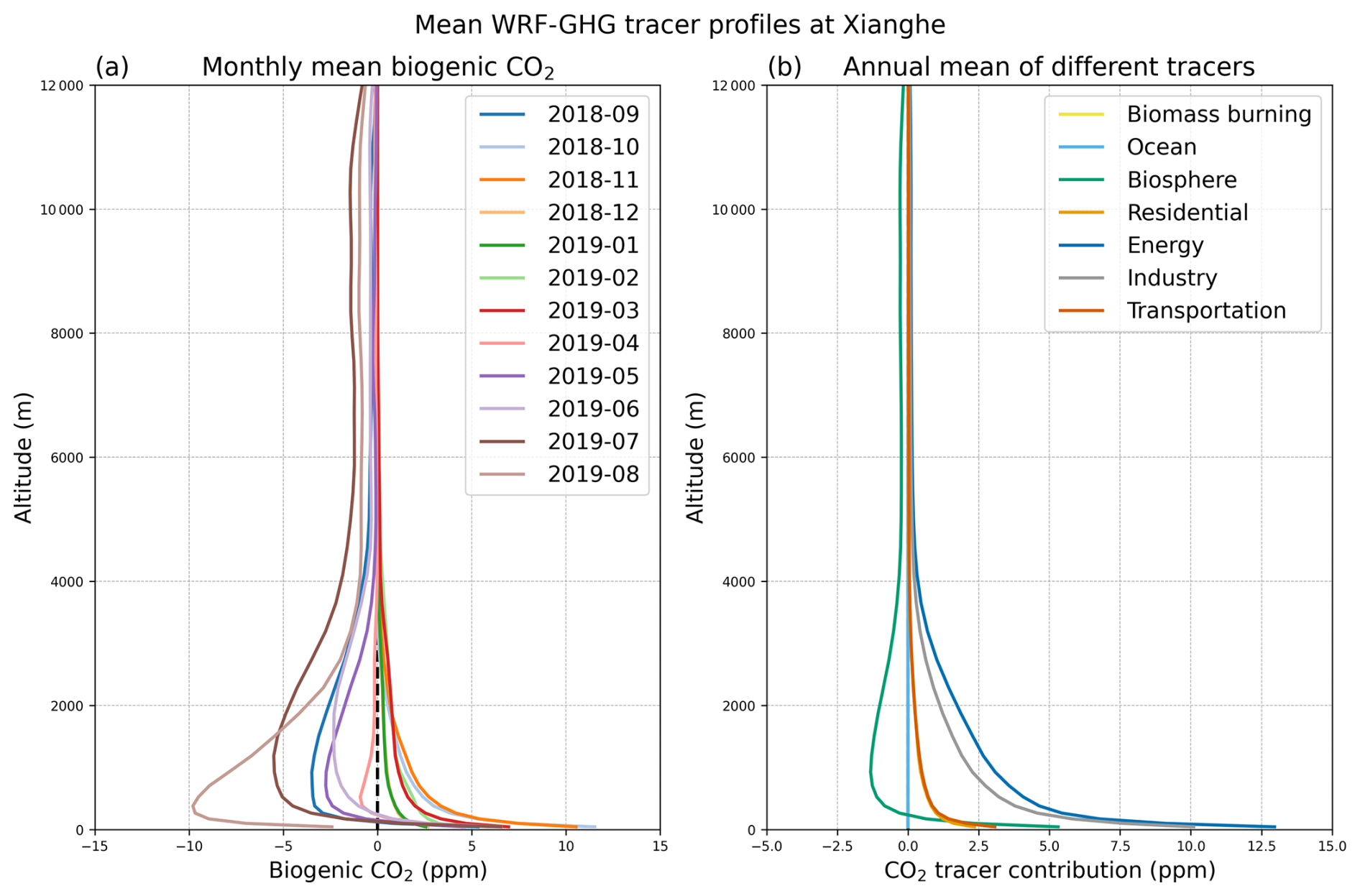
Figure 9 Vertical distribution of simulated CO₂ tracers in WRF-GHG at Xianghe up to 12 km altitude (a) at monthly scale for the biogenic tracer and (b) annual scale for all tracers.

4.2 July XCO₂ anomaly case study

A notable spike in XCO₂ levels is observed between 20–29 July (see Fig. 2a), diverging from the typical decreasing trend of XCO₂ from May to September. We will focus on the model simulations between 7 July and 30 August 2019 to explain the causes of this XCO₂ summer spike, as WRF-GHG correlates well with the observations during this period (correlation coefficient of 0.84).

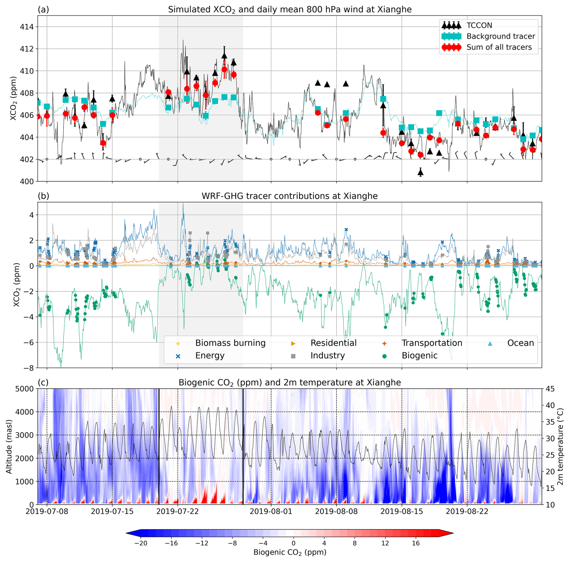
Figure 10 Simulated time series of XCO₂ at Xianghe from 7 July to 30 August 2019, with the spike period highlighted in all panels. Daily mean (a) background tracer (cyan triangles) and total tracers (red diamonds) from WRF-GHG at Xianghe, and TCCON values (black dots). Error bars represent the standard deviation of the daily mean. Daily mean 800 hPa wind direction is indicated by wind barbs at the bottom. (b) Time series of different tracer contributions at Xianghe, with hourly values shown as thin lines and points for TCCON observation times. (c) Color coded vertical profiles of the biogenic CO₂ contributions (left y-axis) shown in red and blue, and surface temperature (right y-axis) in black.

As shown in Fig. 10a, the total simulated XCO₂ increases from 406.30 ± 1.97 ppm before the summer spike (7–19 July) to 408.23 ± 1.67 ppm during the spike (20–29 July), then decreases to 405.01 ± 1.63 ppm afterward (30 July–30 August). These values represent the mean and standard deviation of all hourly WRF-GHG simulated XCO₂ values during each period. Figure 10 shows the simulated background and tracer contributions during this period. Figure 10a shows that the background XCO₂ remains relatively constant in July (406.65 ± 0.93 ppm), and decreases to 405.63 ± 1.19 ppm in August. It further clearly indicates a negative contribution of the tracers before and after the summer spike to a positive enhancement during the spike period. Looking at the different tracers in Fig. 10b, we see that it is mainly the biogenic tracer that has a different behavior in the spike period compared to the periods before and after. Thus, the increase in XCO₂ between 20–29 July is mainly linked to a weaker biogenic sink (−0.86 ± 1.04 ppm) compared to the periods before (−3.56 ± 1.44 ppm) and after (−2.19 ± 1.39 ppm).

Further analysis reveals that during the spike, a heatwave with surface temperatures up to 39 °C occurred, together with 800 hPa winds predominantly from the west (see Fig. 10a and c). The biogenic tracer also shows increased values across a large vertical extent in the troposphere (Fig. 10c), indicating advection from other regions. Synoptic maps (Figs. A2 and A3) show that at the onset of the event, on 20 July 2019, a warm air mass arrived from the northwest. This air mass, originating from the Gobi Desert and grasslands in Inner Mongolia, both areas that are characterized by sparse vegetation and elevated temperatures, carried a lack of biogenic signal and coincides with the jump in the biogenic XCO₂ tracer.

Additionally, the mean NEE around Xianghe, as calculated by VPRM, is slightly higher between 20 and 29 July (average of −5941 mol km⁻² h⁻¹ over domain d03) compared to the periods before and after (respectively −9153 and −12 785 mol km⁻² h⁻¹). In VPRM, the respiration component is linearly dependent on surface temperature, and the gross ecosystem exchange also has a temperature dependency representing the temperature sensitivity of photosynthesis, with CO₂ uptake decreasing at temperatures higher than optimal (Mahadevan et al., 2008). Indeed, it has been shown that extreme temperatures impact CO₂ fluxes (Xu et al., 2020; Ramonet et al., 2020; Gupta et al., 2021).

Therefore, we conclude that the spike was caused by an atmospheric circulation anomaly resulting in the advection of a warm air mass with high biogenic CO₂ levels, followed by locally reduced photosynthesis and increased respiration due to the resulting hot temperatures.

4.3 Sensitivity of near-surface CO₂ simulations to model configuration choices

4.3.1 Emission height

In Sect. 3.4.1, we showed that applying vertical profiles to anthropogenic emissions improved the near-surface CO₂ simulations at Xianghe, substantially reducing the observed nighttime overestimation in the BASE experiment. These findings are consistent with Brunner et al. (2019) and Peng et al. (2023), who highlighted the critical role of emission height in determining near-surface CO₂ mole fractions, particularly under weak mixing conditions. The strong impact on nighttime simulations at Xianghe is likely driven by the proximity of strong point sources (Fig. 5a, b), where the effective release height determines whether emissions remain trapped below or mix above the shallow nocturnal boundary layer.

Nevertheless, some discrepancies with observations remain. In May, for instance, BASE agrees better with observations than PROF, despite May being selected due to poor agreement in the one-year BASE simulation. This apparent contradiction reflects both the short (two-week) duration of the sensitivity runs and the temporal variability of model performance: the main mismatch in BASE occurred in early May, which was not included in the experiments. A full-year sensitivity study would better capture meteorological variability and provide a more robust evaluation, but was not feasible here. The poorer performance of PROF in the second half of May, and the larger MBE in July, remain unexplained, and suggest that further assessment is needed to determine whether the vertical profiles from Brunner et al. (2019) are appropriate for China and consistent with the sectoral and spatial patterns of the emission inventory used in this study.

4.3.2 Land cover representation

Replacing the land-cover dataset with the Copernicus product systematically reduced simulated NEE and nighttime CO₂ mole fractions at Xianghe. This weakening of the biospheric signal is consistent with the larger fraction of non-vegetated land in the Copernicus compared to SYNMAP, leading to smaller VPRM-driven fluxes. The differences are negligible in December and March, when biospheric activity is minimal. While implementing the Copernicus map does not uniformly improve agreement with observations and slightly worsens performance in some periods, it provides a more realistic land-cover representation and is therefore recommended for future regional experiments.

4.3.3 VPRM parameterization

Applying the VPRM parameters from Glauch et al. (2025) produces higher NEE, primarily due to larger α and β values that enhance respiration rates (Table A1). Gross ecosystem exchange (GEE) remains similar between the two configurations, indicating that the net effect is primarily driven by increased respiration rather than changes in photosynthetic uptake. Across all experiments and periods, the PARAM configuration shows the closest agreement with observations, though residual discrepancies suggest that additional model errors remain.

A key limitation is the absence of a standardized VPRM parameter set optimized for China. The only known regional calibration, by Dayalu et al. (2018), introduces seasonal crop subtypes but requires detailed, time-varying land-cover input that is not readily available. Moreover, Seo et al. (2024) reported that the parameter values adopted here (Li et al., 2020) outperform those of Dayalu et al. (2018) over East Asia, supporting our choice.

Recent studies also show that including soil moisture effects in VPRM can improve simulated NEE (Gourdji et al., 2022; Segura-Barrero et al., 2025). However, implementing such modifications would require additional region-specific parameters and could introduce further uncertainty. While the Glauch et al. (2025) parameter set reduces model–observation errors, future work should focus on dedicated VPRM calibration using multi-site eddy-covariance data to develop parameter sets representative of Chinese ecosystems.

4.3.4 Remaining sources of uncertainty

Several factors that were not explicitly tested in this study may still contribute to the remaining biases in simulated near-surface CO₂. One potential source of uncertainty in many regional modeling studies is the coupling between planetary boundary layer (PBL) dynamics and biogenic CO₂ fluxes, a relationship often referred to as the atmospheric CO₂ rectifier effect (Larson and Volkmer, 2008). Since both processes are driven by solar radiation, they interact nonlinearly throughout the diurnal cycle: daytime CO₂ minima result from enhanced turbulent mixing and photosynthetic uptake, whereas nighttime maxima arise from stable stratification and ecosystem respiration. Consequently, accurate simulations require both realistic net ecosystem exchange (NEE) and reliable PBL dynamics. However, in our case, the companion study on CH₄ did not reveal any systematic biases in the mean diurnal cycle, suggesting that PBL processes are reasonably well represented here and unlikely to be the dominant cause of the remaining CO₂ discrepancies. Nevertheless, it is well known that the choice of PBL schemes can have a substantial influence on simulated tracer concentrations (Yu et al., 2022; Kretschmer et al., 2014; Feng et al., 2019; Díaz-Isaac et al., 2018), and uncertainties are generally amplified under weak mixing conditions, such as during the night (Maier et al., 2022). Minor deviations in modeled turbulence or nocturnal stability could therefore still contribute to the observed nighttime biases.

Another contributing factor is the vertical representation of the atmosphere near the surface. Since the observations are collected at 60 m above ground, the simulated CO₂ fields were interpolated to this height. However, in our configuration, the difference in simulated nighttime CO₂ between the two lowest model layers (about 50 and 64 m thick) can reach 20 ppm. This implies that combining an interpolation with too coarse a resolution may introduce errors of several ppm. Increasing vertical resolution within the PBL would help to reduce these artifacts. Overall, the accuracy of near-surface CO₂ simulations depends on the interplay between several model components, including emission height profiles, land cover representation, biogenic flux parameterization, and PBL scheme choice. Improving each of these aspects not only reduces biases but most of all enhances the physical realism of the modeled processes, ultimately leading to more reliable simulations of surface–atmosphere CO₂ exchanges.

5 Conclusions

This study is the second part of a broader investigation into greenhouse gas variability and model performance at the Xianghe site, following earlier work focused on CH₄. Here, we shift the focus to CO₂, aiming to better understand the observed variability through source attribution and model simulations. Using the WRF-GHG model, we performed a one-year simulation of both surface and column-averaged CO₂, evaluated model performance against FTIR and in situ observations, and carried out sensitivity experiments to assess the impact of key model settings.

Model evaluation against FTIR observations at Xianghe shows that WRF-GHG is capable of capturing the temporal variability in column-averaged CO₂ (XCO₂), with a correlation coefficient of 0.7. However, a systematic bias was identified in the model's background CO₂ values from CAMS, with a negative offset exceeding 2 ppm between September and May. After applying a bias correction based on monthly mean CAMS–TCCON differences, the mean bias error was reduced to −0.86 ppm. These findings underscore the importance of accurate boundary conditions when simulating XCO₂, particularly due to the long atmospheric lifetime of CO₂ and the relatively small contribution of regional emissions to the total column. In our simulations, emissions within the model domain contributed only ∼1.82 ppm to XCO₂, making the column signal highly sensitive to background mole fractions. Furthermore, the model successfully captured a strong positive anomaly observed in July 2019, attributed to the advection of a warm, CO₂-rich air mass. This case study illustrates the value of combining transport and mole fraction diagnostics for interpreting episodic events in column data and highlights the dominant role of synoptic meteorology in driving short-term variability in XCO₂.

For near-surface CO₂ mole fractions, WRF-GHG shows good agreement with afternoon observations at Xianghe, achieving a correlation coefficient of 0.75 and a mean bias error of −2.44 ppm after bias correction. In contrast to XCO₂, near-surface CO₂ was more strongly influenced by local sources, with a mean tracer enhancement of 26.78 ppm, resulting in a smaller relative importance of boundary condition errors. Nighttime mole fractions are consistently overestimated, with a mean bias of 7.86 ppm and a lower correlation of 0.60. These discrepancies are reflected in the diurnal cycle: while the model captures the overall structure driven by planetary boundary layer dynamics, it overestimates the daily amplitude of 22.1 ppm by 4.58 ppm. Likely causes include inaccuracies in NEE and the vertical distribution of anthropogenic emissions.

Additional sensitivity experiments show that applying vertical emission profiles and a more recent land cover map can reduce nighttime CO₂ mole fractions and improve agreement with observations. Adjustments to the VPRM vegetation parameters substantially affected near-surface mole fractions, with differences up to 10 ppm, underscoring the critical role of appropriate parameter selection–especially in the absence of a standardized VPRM configuration for China.

Tracer analysis confirms that the industry and energy sectors are the dominant contributors to CO₂ levels at Xianghe, while the biosphere plays a secondary, seasonal role. For XCO₂, the biosphere acts as a sink from April to September (−0.77 ppm on average) and a weak source in the remaining months (+0.22 ppm). At the surface, biospheric uptake is only seen in August (−6.76 ppm), while respiration dominates the rest of the year (+2.69 ppm on average). These differences illustrate the greater local sensitivity of in situ measurements compared to column observations and the varying spatial influence of different source types.

Overall, this study demonstrates the value of using a modeling framework like WRF-GHG to interpret both temporal and sectoral variations in surface and column CO₂ observations. It also highlights that model accuracy is strongly dependent on appropriate configuration choices, including the representation of boundary conditions, vertical emission profiles, and biogenic flux parameterizations. Addressing these factors is essential for improving simulations and supporting more accurate source attribution of observed CO₂ variability.

Appendix A: Additional tables and figures

Figure A1 Same as Fig. 2 but showing the original (not bias corrected) model values.

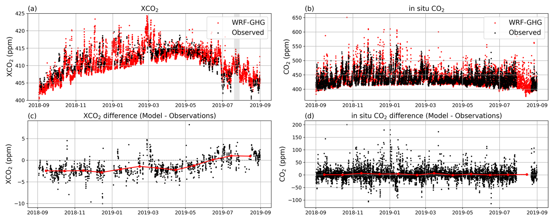
Table A1 VPRM parameter values for different vegetation classes.

Table A2 Same as Table 5 but for XCO₂.

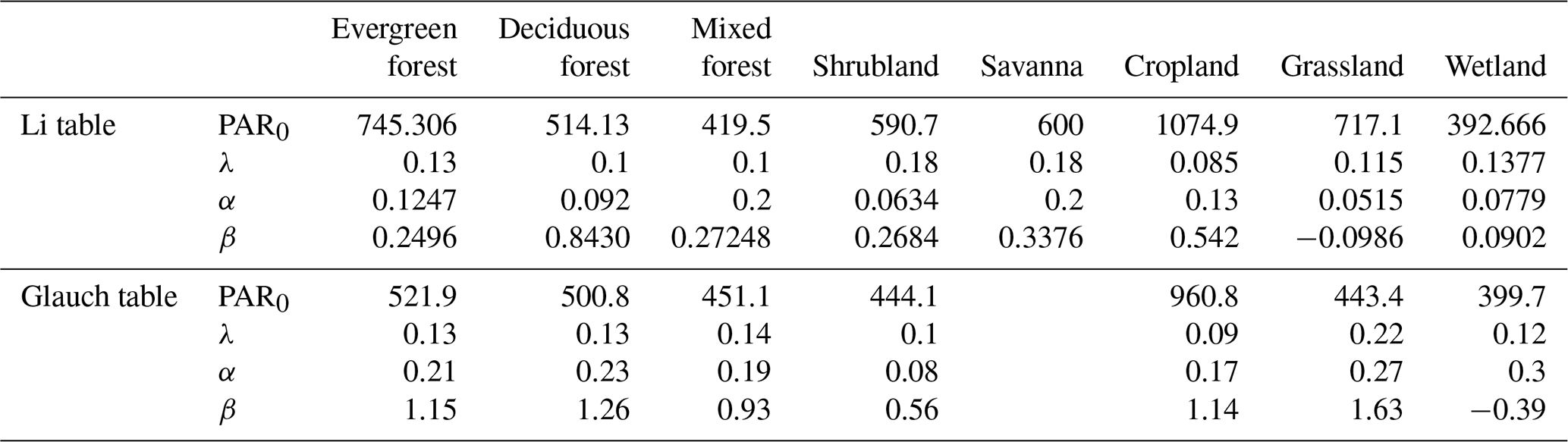
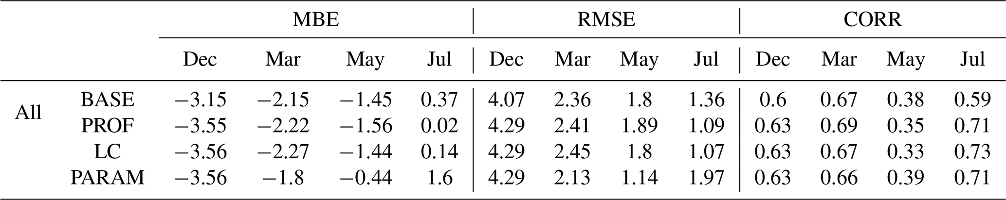
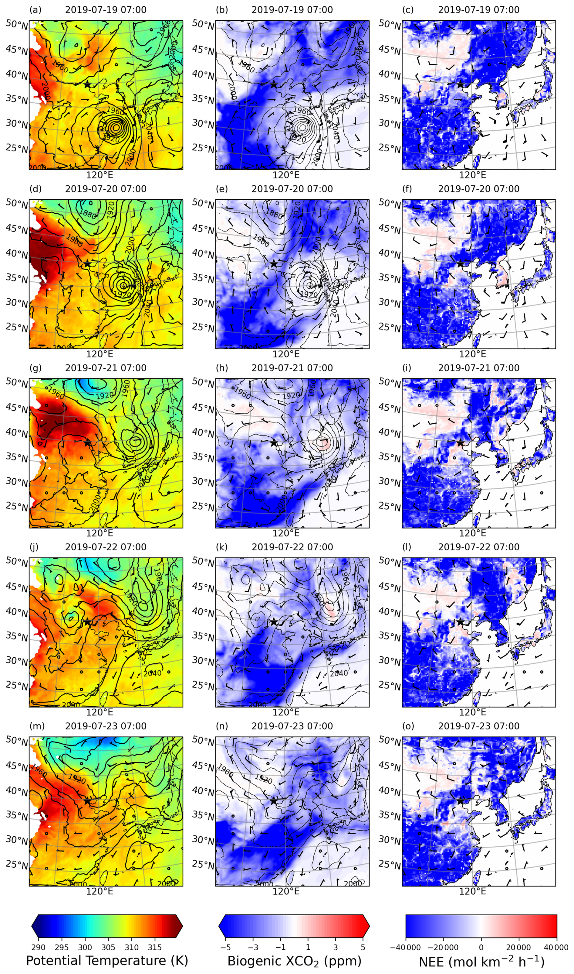
Figure A2 Maps of eastern China at 800 hPa for 19–23 July 2019, 07:00 UTC (15:00 LT). Panels in the first column show potential temperature (K, in color) with wind barbs and geopotential height contour lines at 800 hPa (contour interval every 20 m); panels in the second column show biogenic XCO₂ enhancements (ppm, in color) with the same wind vectors and contours; the third column shows the NEE. The Xianghe site is marked by a black star.

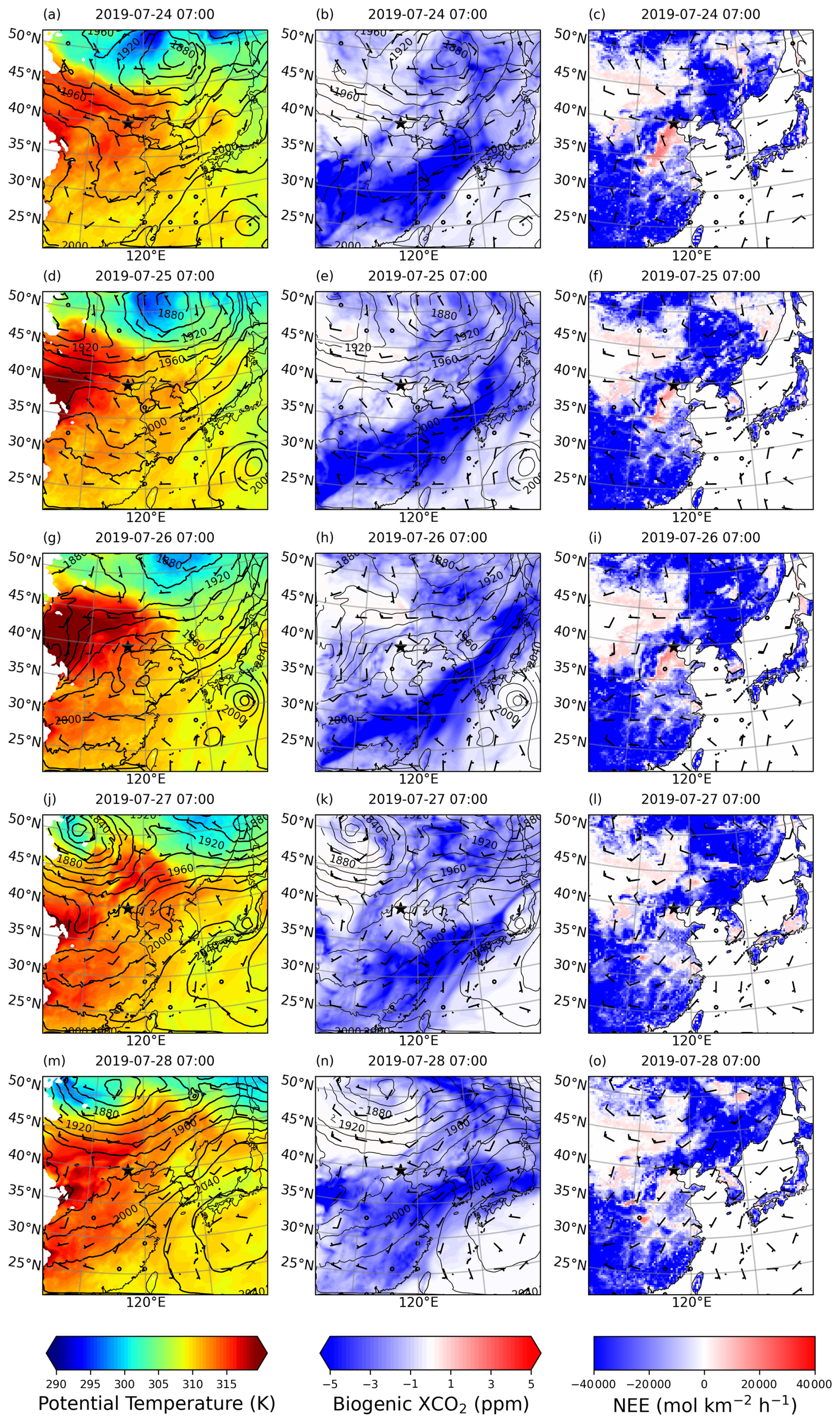
Figure A3 Same as Fig. A2 but over the period 24–28 July 2019.

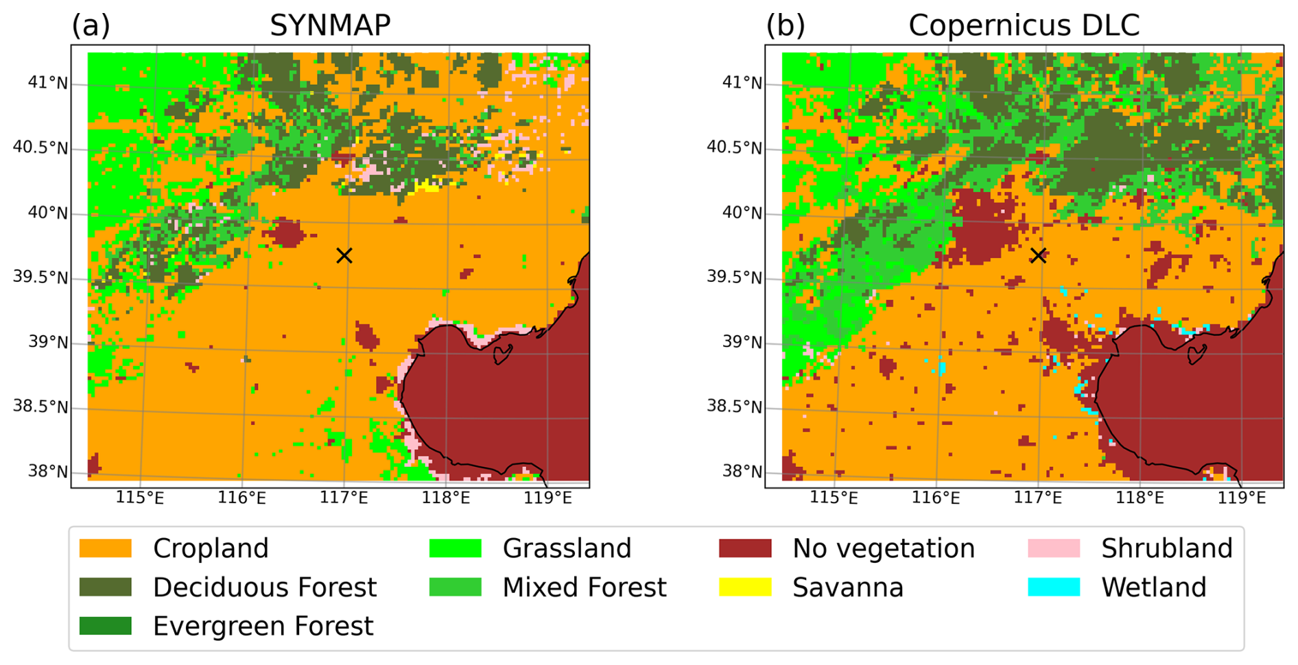
Figure A4 Dominant VPRM vegetation category in WRF-GHG domain d03 (3 km) for (a) 1-km SYNMAP and (b) 100-m Copernicus Dynamic Land Cover Collection 3 (epoch 2019). The black cross indicates the location of the Xianghe site.